Automated Segmentation and Quantification of Histology Fragments for Enhanced Macroscopic Reporting

Abstract

Manual tissue documentation is a critical step in the field of pathology that sets the stage for microscopic analysis and significantly influences diagnostic outcomes. In routine practice, technicians verbally dictate descriptions of specimens during gross examination; these are later transcribed into macroscopic reports. Fragment sizes are measured manually with rulers; however, these measurements are often inconsistent for small, irregular biopsies. No photographic record is captured for traceability. To address these limitations, we propose a proof-of-concept framework that automates the image capture and documentation of biopsy and resection cassettes. It integrates a custom imaging platform and a segmentation pipeline leveraging the YOLOv8 and YOLOv9 architectures to improve accuracy and efficiency. The framework was tested in a real clinical context and was evaluated on two datasets of 100 annotated images each, achieving a mask mean Average Precision (mAP) of 0.9517 ± 0107 and a tissue fragment spatial accuracy of 96.20 ± 1.37%. These results demonstrate the potential of our framework to enhance the standardization, reliability, and speed of macroscopic documentation, contributing to improved traceability and diagnostic precision.

1. Introduction

Histology is a cornerstone of medical diagnostics, offering insights into the structure and pathology of biological tissues. Before microscopic examination, tissues undergo macroscopic analysis in a crucial initial step that is known as gross examination. During this stage, pathologists visually inspect, measure, and describe tissue samples with the naked eye. This phase is fundamental, setting the stage for microscopic analysis and ultimately influencing diagnostic outcomes [1]. To provide context and clarity on the overall workflow, Figure 1 illustrates the sequential steps involved in histological tissue processing, from sample reception to digital slide visualization.

1.1. Gross Examination Technologies

Gross examination is a complex, highly demanding process that requires a deep understanding of anatomical structures, the careful orientation of specimens, and meticulous attention to detail. It encompasses challenges such as accurately identifying anatomical structures, recognizing subtle abnormalities, and carefully selecting regions for further microscopic study. Pathologists face additional pressures due to the increasing volume of biopsies and surgical specimens, combined with the demand for rapid turnaround times [2]. Meeting these demands not only requires advanced skills in tissue sectioning and handling but also necessitates the ability to accurately interpret tissue samples.

The accuracy of gross examination relies on detailed documentation and precise communication, as each measurement, description, and observation directly impacts patient outcomes. Moreover, this process involves safety risks, including exposure to infectious materials and the handling of hazardous chemicals, necessitating strict adherence to protocols [3]. The grossing room environment is physically and emotionally taxing, requiring long periods of focused concentration and the handling of distressing specimens, which adds further complexity to the role [4].

In current pathology laboratories, macroscopic reporting is typically performed through verbal dictation by the technician, while manipulating the specimens. These audio recordings are later transcribed by staff to generate the final macroscopic report. For biopsy samples, the number of tissue fragments per cassette is counted and their sizes are measured approximately using a ruler. Because biopsy fragments are often very small and have irregular shapes, each technician tends to develop their own way of estimating dimensions, introducing significant variability. In the case of surgical resections, the reported dimensions may correspond either to the intact specimen before sectioning or to the individual fragments placed into the cassette. This process remains largely manual and is not standardized, especially in relation to how fragment dimensions are recorded. Critically, no images of the cassettes are captured or archived, limiting traceability and making it difficult to verify documentation accuracy or to retrospectively detect sampling errors.

To address these challenges, recent technological advancements have introduced automation in gross examination, integrating digital imaging, automated specimen processing, and laboratory information systems. Automated systems such as the VistaPath Sentinel [5] and FormaPath nToto [6] leverage artificial intelligence and computer vision to reduce human error, accelerate processing times, and standardize documentation. For instance, the VistaPath Sentinel has demonstrated a 93% faster gross reporting speed, while improving accuracy by 43% through continuous video monitoring and AI-based error reduction. Similarly, the FormaPath nToto system, which was designed for smaller biopsy samples, fully automates the transfer and documentation process, showing promising results in pilot tests at the Mayo Clinic.

Additionally, systems such as the Tissue-Tek AutoTEC a120 [7,8,9] automate the tissue embedding process, eliminating the need for manual orientation. The eGROSS pro-x [10], which is an advanced grossing workstation, integrates digital specimen identification with image documentation, creating a standardized, hands-free workflow with enhanced traceability and efficiency. These technologies collectively represent a shift toward precision, consistency, and workflow integration, addressing many traditional challenges in gross examination.

To summarize the capabilities and limitations of existing solutions,

Table 1. Comparison of existing automated gross examination technologies.

System	Functionality	Advantages	Limitations
VistaPath Sentinel [5]	AI-powered augmentation system for grossing	Reduces grossing time by 93%; improves labeling accuracy by 43%	High cost; requires extra space for device and display in grossing station
FormaPath nToto [6]	Automated transfer and documentation of small biopsies using computer vision and robotics	Hands-free documentation; suitable for biopsies < 1 cm2; tested in clinical settings	Limited to small biopsies; not suitable for large or complex specimens
eGROSS [10]	Digital macro documentation with integrated high-resolution imaging, audio, and traceability tools	Enhances traceability with high-resolution images and voice notes; useful for education and audits	Limited portability; not easily adaptable to compact or space-constrained grossing areas

provides a comparative overview of recent automated gross examination technologies.

While current automation tools offer significant benefits, many remain costly, bulky, or unsuitable for smaller laboratory settings. There is a need for compact, cost-effective solutions that can improve the accuracy of tissue documentation while seamlessly integrating into diverse lab workflows. Our study aims to address this need by introducing a framework for grossing workstations, enabling the automated image capture and documentation of biopsy and resection cassettes. This framework segments tissue fragments and provides their number and dimensions, improving traceability, reducing the documentation burden, and assisting technicians in their daily workflows.

We use instance segmentation to identify and outline tissue fragments. The next section reviews the evolution and use of the You Only Look Once (YOLO) family of algorithms that have proven effective in similar medical imaging applications.

1.2. Instance Segmentation Overview

Instance segmentation, which is a computer vision task that combines object detection (class-wise localization) and semantic segmentation (pixel-wise classification), is used to identify and delineate individual objects within an image at the pixel level. This makes instance segmentation suitable for applications where the outline of objects and their spatial distribution matter. Real-time instance segmentation has emerged as a transformative technology in healthcare applications, revolutionizing medical image analysis and clinical decision-making processes [11,12]. As healthcare systems increasingly adopt artificial intelligence and machine learning solutions, the ability to precisely delineate and identify individual objects or structures in medical imaging has become paramount. The integration of advanced segmentation techniques has enabled healthcare professionals to achieve more accurate diagnoses and to implement targeted interventions with unprecedented precision [13].

Real-time object detection has been revolutionized by the YOLO series of algorithms, since their inception in 2016. Iterative advancements from YOLOv1 to YOLOv12 have introduced significant architectural improvements, continually enhancing detection performance. Each version has addressed specific challenges, including improving accuracy, handling small objects, and increasing processing speed for real-time applications.

YOLOv1 [14] distinguished itself by unifying localization and classification within a single network pass, demonstrating a departure from conventional two-stage detectors such as R-CNN. While offering a speed advantage, its limitations included difficulty in detecting smaller objects and various spatial constraints imposed by its fixed grid system. YOLOv2 [15] addressed these issues by introducing anchor boxes, batch normalization, high-resolution fine-tuning, and k-means-derived anchor dimensions via the Darknet-19 backbone. These additions significantly reduced computational complexity compared to YOLOv1’s GoogLeNet-based architecture, while also improving precision. YOLOv3 [16] is characterized by a further refined architecture, with multi-scale detection (utilizing 13 × 13, 26 × 26, and 52 × 52 grids), a Darknet-53 backbone incorporating residual connections, and binary cross-entropy loss; this resulted in an improved precision and reduced latency.

Subsequent versions continued to optimize the algorithm’s performance. YOLOv4 [17] enhanced training efficiency with Mish activation, spatial attention modules, and Complete IoU (CIoU) loss. Furthermore, YOLOv5 [18] prioritized deployment via PyTorch implementation, AutoAnchor optimization, and mosaic augmentation, scaling parameter counts from 1.9 million to 86.7 million. YOLOv6 [19] focused on edge performance optimization with EfficientRep reparameterization, an anchor-free design, and SCYLLA IoU (SIoU) loss, enabling a processing speed of 1242 FPS on T4 GPUs. The architecture of YOLOv7 [20] was refined through Extended-Efficient Layer Aggregation Network (E-ELAN) blocks and dynamic label assignment.

Moreover, YOLOv8 [21] expanded the algorithm’s capabilities to include instance and panoptic segmentation, as well as keypoint estimation, through task-specific heads and anchor-free prediction. In subsequent iterations, YOLOv9 [22] introduced programmable gradient information (PGI) and the Generalized Efficient Layer Aggregation Network (GELAN). In addition, YOLOv10 [23] emphasized parameter efficiency through omni-dimensional convolution and rank-based pruning. Meanwhile, YOLOv11 [24] unified multi-task support for rotated objects and pose estimation, while YOLOv12 [25] integrates attention modules with Residual Efficient Layer Aggregation Networks (R-ELANs).

A comprehensive review of YOLO algorithms highlights their growing significance in relation to various medical applications [26]. In the field of biomedical research, an optimized version of YOLOv7, enhanced by the Cheetah Optimization Algorithm for anchor box selection, was utilized in droplet-based microfluidic systems for detecting and analyzing droplets [27].

In dermatology, YOLOv7 has proven effective in distinguishing between malignant melanomas and benign skin lesions, achieving an Intersection over Union (IoU) of 86.3%, a mean Average Precision (mAP) of 75.4%, and an F1-measure of 77.9%, all within an inference time of just 0.31 s per image [28]. Similarly, Histology-based Detection using YOLO (HD-YOLO) has revolutionized pathology by enhancing the speed and accuracy of nucleus segmentation and tumor microenvironment analysis in whole-slide tumor imaging. This approach has demonstrated superior prognostic relevance in cancers such as lung, liver, and breast in comparison to traditional histological markers [29].

In more clinical applications, a CNN-based framework employing the YOLO architecture, along with Gunnar Farneback motion estimation and Assisted Excitation for imbalanced data handling, has been developed for ultrasound-guided interventions. This technology significantly improves visibility and accuracy in needle placement, enhancing procedural outcomes [30]. For drug administration, YOLOv3’s detection speed makes it suitable for real-time use in hospitals for pill identification [31].

Furthermore, for brain tumor detection and segmentation in MRI scans, a combination of YOLO-CNN for detection and FCN-UNet for segmentation achieved a correct classification ratio of 97% across various testing scenarios [32]. The YOLOv5 model, which can be used within a portable microwave head imaging system, has shown promising results in real-time applications for distinguishing between benign and malignant tumors [33]. In magnetic resonance imaging (MRI), studies evaluating the YOLOv5 and YOLOv7 models have demonstrated their potential to enhance tumor detection and segmentation [34]. Finally, YOLOv8’s capabilities extend to detecting dental abnormalities such as cavities, periodontal disease, and oral cancers [35], highlighting its versatility in medical imaging.

Table 2. YOLO-based instance detection and segmentation applications in medical imaging.

Application Area	YOLO Version	Imaging Modality	Key Metrics/Highlights
Microfluidic droplet detection for biomedical research [27]	YOLOv7	Microscopic images of microfluidic droplets	Achieves 96% accuracy and 93% F1-score. Uses Cheetah Optimization Algorithm for optimal selection of anchor boxes.
Skin cancer recognition [28]	YOLOv3, YOLOv4, YOLOv5, YOLOv7	Dermoscopy images	Experimental results show that the YOLOv7 model achieves the best performance—IoU: 86.3%, mAP: 75.4%, and F1: 77.9%.
Nucleus detection, segmentation, and classification [29]	HD-YOLO	WSI	Achieved an F1-score of 0.7409 and a mean Intersection over Union (mIoU) of 0.8423 in lung cancer detection.
Needle tracking in ultrasound interventions (biopsies, epidural injections) [30]	Modified YOLOv3 (nYolo)	Ultrasound	Uses spatiotemporal features of speckle dynamics to track needles, especially when they are invisible. Achieved angle and tip localization errors of $2.08\pm 1.18°$ and $2.12\pm 1.43$ mm, respectively, in challenging scenarios.
Real-time pill identification [31]	YOLOv3	RGB pill images	Addresses the issue of pharmacists struggling to distinguish pills due to the lack of imprint codes. Compares YOLOv3 to RetinaNet and SSD to reduce medication errors and the waste of medical resources. YOLOv3 achieved the best mAP of 93.4%.
Brain tumor detection and segmentation [32]	YOLO + FCN-UNet	MRI	Achieved a correct classification rate of about 97% using YOLOv3-UNet for segmenting original and Gaussian noisy images. YOLOv4-UNet performed less satisfactorily.
Brain abnormality detection and classification [33]	YOLOv5	Reconstructed microwave brain images	The YOLOv5l model performed better than YOLOv5s and YOLOv5m, acheiving an 85.65% Area Under the Curve (AUC) for benign tumor classification and a 91.36% AUC for malignant tumor classification.
Brain tumor segmentation and classification [34]	YOLOv5, YOLOv7	MRI	The models were trained and validated on the Figshare brain tumor dataset. YOLOv5 achieved a box mAP of 0.947 and a mask mAP of 0.947, while YOLOv7 achieved a box mAP of 0.940 and a mask mAP of 0.941.
Dental radiography analysis [35]	YOLOv8	Panoramic dental radiography	Precision of 82.36% in detecting and classifying dental diseases (cavities, periodontal disease, oral cancers).

summarizes the use of YOLO-based models across diverse medical imaging domains.

Despite the success of instance segmentation in various medical imaging tasks, its application to gross examination remains limited. Most current implementations focus on microscopic or radiological images. In the context of macroscopic pathology, no affordable solution currently leverages segmentation to quantify tissue fragments directly from cassette images. This gap in workflow integration and traceability motivates our proposed framework.

1.3. Contributions

The primary objective of this study is to present a novel framework designed for pathology laboratories to automate and standardize the documentation and reporting of tissue fragments within cassettes. This framework integrates a purpose-built imaging platform and an instance segmentation pipeline. Our key contributions include the following:

• The design and implementation of a compact, 3D-printed imaging platform specifically engineered for tissue fragment documentation.
• The creation of a comprehensive dataset of biopsy and resection fragments, meticulously annotated using the Segment Anything Model (SAM).
• The integration of a YOLO-based instance segmentation approach for the detection and segmentation of tissue fragments.
• The automatic generation of visual reports summarizing the number and size of detected fragments to support quality control in pathology workflows.

The structure of this paper is as follows: Section 1 provides a literature review that establishes the research context and highlights existing technologies. Section 2 outlines the methodology, detailing the tissue fragment documentation system, including data collection, preprocessing, segmentation models, and performance assessment. Section 3 presents the experimental results, evaluating the system’s effectiveness. In Section 4, we discuss the findings and propose directions for future work. Finally, Section 5 summarizes the key contributions and outcomes of this study.

2. Materials and Methods

The histopathology image capture and processing platform is based on a sequential, multi-step process. This process begins with the physical capture of images of tissue fragments within cassettes, followed by the recognition of an identifier using Azure Optical Character Recognition (OCR) technology [36]. Subsequent data annotation is performed using SAM to delineate specific regions, which is essential for training a YOLO-based segmentation model (Yolo-seg) to automatically segment tissue fragments. The full pipeline is illustrated in Figure 2.

2.1. Cassette Image Capture Platform

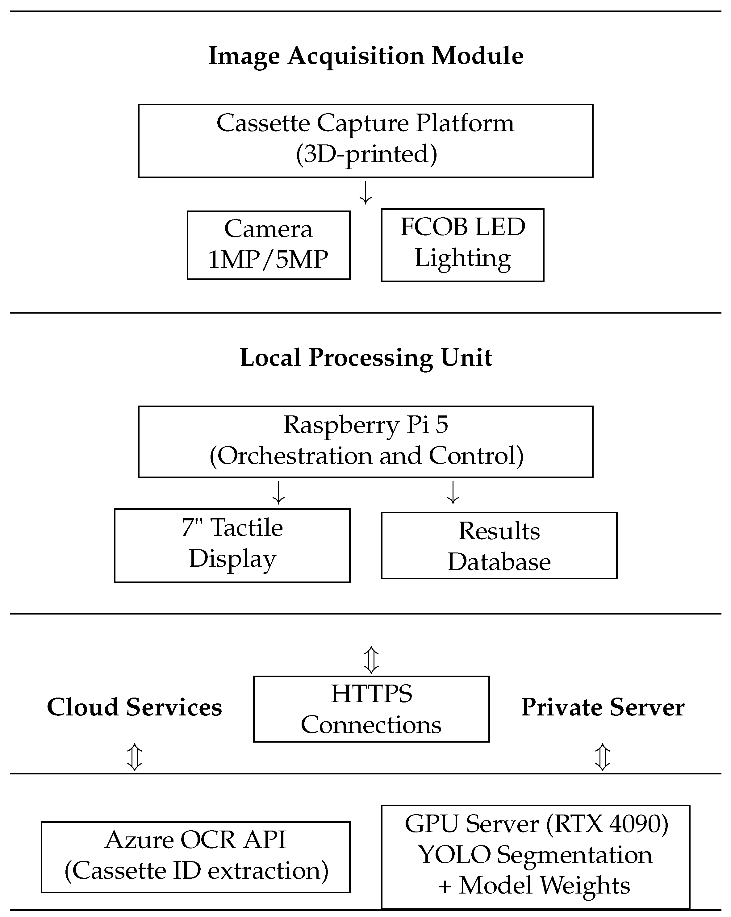
The primary objective of the cassette image capture platform is to standardize the capture of cassettes for our database, ensuring consistency in lighting, positioning, and image quality. Figure 3 illustrates the complete technological infrastructure of the automated tissue documentation framework. The architecture follows a modular design with the following three main components: (1) the image acquisition module with standardized lighting and positioning; (2) the local processing unit with Raspberry Pi for capture control, result display, and data transmission; and (3) the remote processing server for computationally intensive segmentation tasks, coordinating with Azure cloud services for OCR-based ID extraction.

The selection of each component was based on comparisons with alternatives, as detailed in

Table 3. Justification of hardware and software components based on performance, cost, and applicability to histology.

Component	Justification	Alternatives Considered	Reason for Exclusion
Raspberry Pi 5	Compact; low power consumption; Linux support; sufficient for image capture and display control	NVIDIA Jetson Nano, Arduino	Jetson Nano not tested due to higher cost; Arduino lacks support for complex vision tasks
HBV-W202012HD Camera (1 MP)	Minimal optical distortion; stable USB interface; cost-effective; no calibration needed	5 MP Raspberry Pi Camera	Minimal accuracy improvement; increased processing time and storage requirements
Custom Light Box with FCOB LED Strip	Uniform illumination achieved through custom-built diffusion box integrated into 3D-printed platform	Ring light	Ring light difficult to integrate into compact design
Touchscreen Interface	Direct interaction for technicians; immediate result validation; compact integration	External monitor; mobile app	Monitor requires peripherals and larger footprint; mobile app needs network setup and device management
3D-printed PLA Platform	Cost-effective; easily customizable; rapid prototyping	Nylon (3D printing)	Nylon is difficult to print and is prone to warping
Azure OCR API	High accuracy on cassette text; handles various orientations	Tesseract OCR; EasyOCR; PaddleOCR	Lower accuracy on cassette IDs; Tesseract required extensive preprocessing; PaddleOCR and EasyOCR showed inconsistent character recognition

. Our decisions prioritized cost-effectiveness, reliability, and seamless integration within existing pathology workflows.

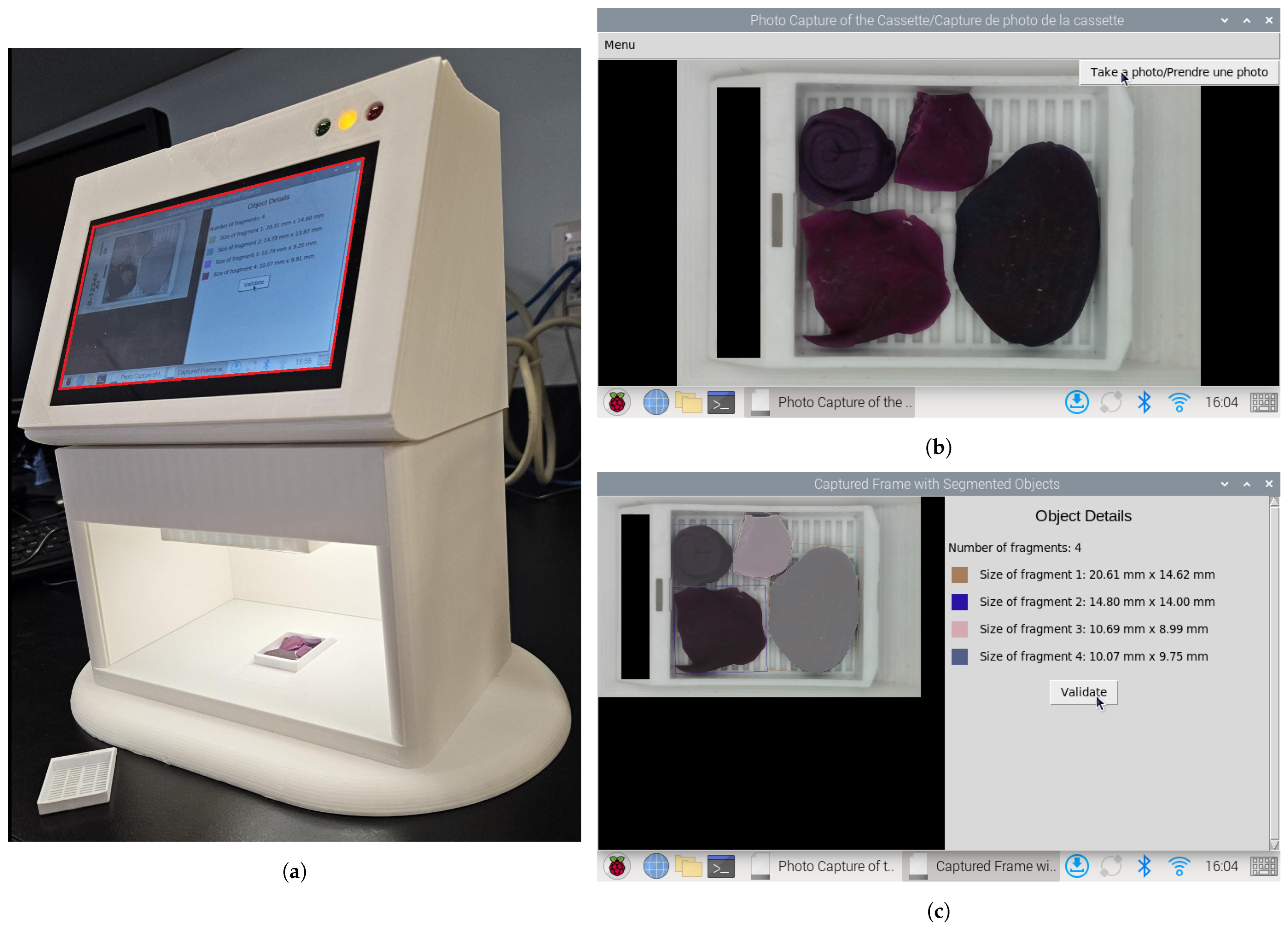
The prototype of the cassette image capture platform was designed using Autodesk Fusion 360, which is a leading 3D modeling software, in order to ensure precision in dimensions and component placement. The design features an open side to facilitate the insertion of cassettes into a designated slot measuring 40 × 28 cm. The prototype was produced using an Ultimaker S7 3D printer, which allowed for the high-resolution and durable construction of the box components from Polylactic Acid (PLA).

Illumination within the box is provided by a lighting enclosure positioned directly above the cassette within the main box. This enclosure houses a flexible circuit board (FCOB) LED strip light, which offers ample lighting and uniform light distribution across different times of the day and under varying ambient lighting conditions. A diffusing sheet covers the LEDs to soften the light, reducing glare that could affect the image quality.

Positioned above the cassette slot, an HBV-W202012HD USB camera captures high-definition images. This camera, with a resolution of 1 megapixel (MP), was selected for its clarity, cost-effectiveness, and minimal distortion, which allows for real-time processing without the need for computational correction.

To evaluate the impact of resolution and processing time, a second camera—the 5 megapixel OmniVision OV5647 sensor of the original Raspberry Pi Camera Module—was also tested. Although this higher-resolution module provided more image detail, its lens distortion required additional software correction through undistortion techniques, which increased processing time.

The platform includes a Raspberry Pi 5 Model B, which has demonstrated its effectiveness in many studies [37]; it also includes a tactile interface screen, facilitating the seamless integration of hardware and software components. This setup allows for the direct transmission of images from the platform to a remote server. Once the images are uploaded, the instance segmentation model processes them to determine the number and dimensions of fragments present. The results are then sent back to the local system, displaying them on the tactile screen for immediate review. This efficient communication setup ensures that the data processing is both rapid and reliable.

2.2. Patient Identifier Processing and Data Security

Azure OCR technology is utilized to automatically extract the cassette identifier. Any personal information on the cassette is obscured to comply with data protection regulations. The images, with anonymized content, are then saved in the database using the identifier as the file name. This process ensures that each image is uniquely linked to its corresponding cassette without exposing personal information, maintaining strict data security and privacy standards.

2.3. Data Annotation

The annotation of the images captured by our cassette photography box was conducted using the Segment Anything Model (SAM) [38]. The SAM is a promptable model that was developed by Meta AI Research. The model aims to provide a segmentation mask using any segmentation prompt, which includes text or spatial information about the desired object. The annotated data were then utilized to train the instance segmentation model, which is designed to identify and delineate each fragment within the cassette images.

2.4. Fragment Segmentation

To aid grossing examination technicians in generating macroscopic reports by providing accurate counts and measurements of fragment dimensions within cassettes, we fine-tuned the latest pre-trained versions of YOLO models for identifying and delineating these fragments. YOLOv8 and YOLOv9, which were employed in our experiments, are state-of-the-art models for object detection and instance segmentation. These versions significantly enhance accuracy, processing speed, and overall efficiency.

2.4.1. Yolov8 Instance Segmentation Architecture

The YOLOv8-seg architecture represents a significant evolution in relation to real-time instance segmentation [21]; this architecture was launched in 2023. YOLOv8 integrates advanced architectural features to improve feature extraction and fusion. These features are as follows:

• Cross-Stage Partial Darknet (CSPDarknet) backbone
  The backbone employs a modified CSPDarknet architecture that integrates CSP modules to reduce computational redundancy while enhancing gradient flow. The CSP design in YOLOv8 splits the feature map of each stage into two parts, with one part undergoing a dense block of convolutions and the other being directly concatenated with the dense block’s output, reducing computational complexity while preserving accuracy. The backbone consists of multiple CSP blocks, each comprising a split operation, a dense block, a transition layer, and a concatenation operation. YOLOv8 also utilizes Sigmoid Linear Unit (SiLU) for non-linear feature mapping, which enhances gradient flow and feature expressiveness. These design elements reduce computational complexity, improve gradient flow, enhance feature reuse, and maintain high accuracy while reducing model size. The backbone generates feature maps at three scales (P3, P4, and P5) with strides of 8, 16, and 32 pixels, respectively, thus capturing hierarchical spatial information from fine-grained details to high-level semantics.
• Path Aggregation Network (PANet) neck
  The PANet neck in YOLOv8 enhances information flow and feature fusion across different network layers by building on the Feature Pyramid Network (FPN) design. It includes a bottom-up path for feature extraction, a top-down path for semantic feature propagation, and an additional bottom-up path for further feature hierarchy enhancement. At each level, features from corresponding bottom-up and top-down paths are fused through element-wise addition or concatenation, while adaptive feature pooling is introduced to enhance multi-scale feature fusion by pooling features from all levels for each region of interest. This design improves the network’s ability to detect objects at various scales, boosts performance relating to small object detection, and enhances information flow between different feature levels, making it crucial for edge applications where objects may appear at different scales and distances.
• Detection and segmentation heads
  The detection–segmentation head operates through two parallel branches. The detection branch uses an anchor-free mechanism to predict center points via a 1 × 1 convolution with 4 + C4 + C outputs (box coordinates, objectness, and class probabilities). Its loss function combines Distribution Focal Loss (DFL) for classification and CIoU for regression. The segmentation branch includes a mask prototype network that generates 32 prototype masks per image through a 3 × 3 convolution layer. Mask coefficients are predicted alongside detection outputs and are combined through matrix multiplication. The segmentation branch’s loss function uses binary cross-entropy.

The key features that make YOLOv8 well-suited for fragment segmentation include the Cross Stage Partial with Two Fusion (C2f) building block, which enhances feature extraction and fusion. This improves the model’s ability to capture fine-grained details and complex patterns, which are essential for accurate segmentation. Additionally, the Spatial Pyramid Pooling Fast (SPPF) module enables efficient multi-scale feature extraction by applying max-pooling operations at different scales. This allows YOLOv8-seg to recognize objects more effectively, even in images containing fragments of varying sizes.

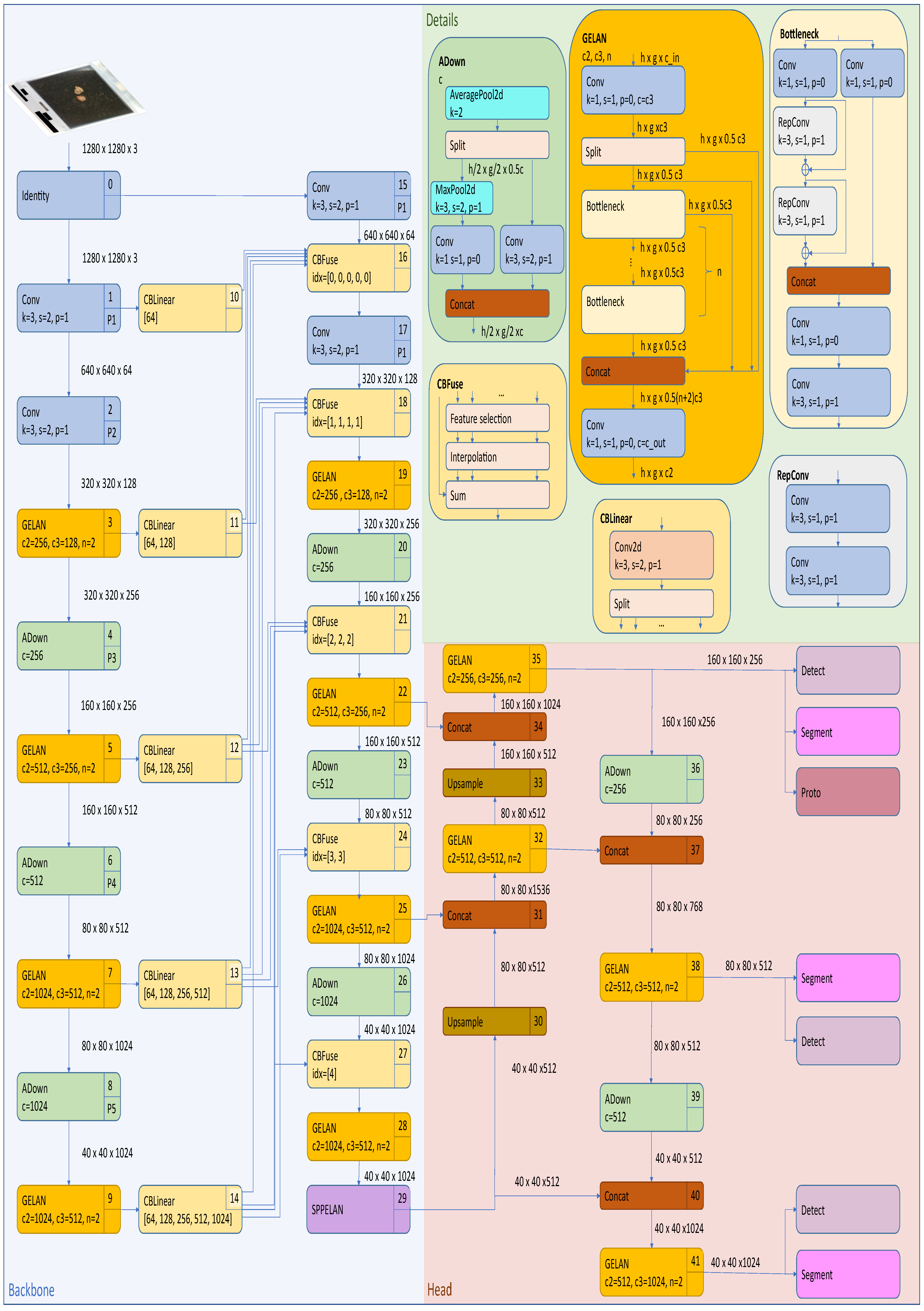
Figure 4 presents the YOLOv8-seg architecture as implemented in our instance segmentation pipeline. This architecture was extended and adapted from the Ultralytics YOLOv8 architecture diagram [39] based on the code implementation used in our experiments. Our adaptations included modified input sizes for our specific cassette imaging requirements, while extensions included the segmentation modules for instance segmentation functionality.

2.4.2. Yolov9 Instance Segmentation Architecture

YOLOv9-seg is an advanced object detection and segmentation model that builds upon the YOLOv9 architecture [22]. Here, we provide a detailed overview of its architecture:

• Generalized Efficient Layer Aggregation Network (GELAN) backbone
  The backbone in YOLOv9-seg is designed to extract multi-scale features from the input image. It leverages the GELAN, which combines the strengths of CSPNet and the Efficient Layer Aggregation Network (ELAN). GELAN incorporates various computational blocks such as CSPblocks, Resblocks, and Darkblocks, ensuring efficient feature extraction while preserving key hierarchical features across the network’s layers.
• Programmable Gradient Information (PGI) neck
  The neck component in YOLOv9-seg enhances the feature fusion process using PGI; this introduces an auxiliary reversible branch that ensures reliable gradient flow across the network, addressing the problem of information loss during training. This reversible architecture ensures that no crucial data are lost during the forward and backward passes, leading to more reliable predictions.
• Detection and segmentation heads
  The head in YOLOv9-seg utilizes an anchor-free bounding box prediction method, similar to that of YOLOv8, but also benefits from the reversible functions provided by PGI. The head is divided into two parts—the main branch and the multi-level auxiliary branch. The auxiliary branch focuses on capturing and retaining gradient information during training, supporting the main branch by preserving essential gradient information.

In addition to object detection, YOLOv9-seg includes a segmentation branch that allows the model to perform instance segmentation. This branch processes the feature maps generated by the backbone and neck to produce segmentation masks for detected objects. The segmentation branch is designed to work seamlessly with the detection head, ensuring that both tasks benefit from the shared feature extraction process.

To avoid redundancy, the overall backbone structure of YOLOv9e-seg shares many components with YOLOv8-seg, as illustrated in Figure 4. Therefore, only the architecture-specific modifications are detailed in Figure 5. An architectural difference lies in the use of the SPPELAN module, which replaces the SPPF module found in YOLOv8. While SPPF uses fixed intermediate channels (typically half the number of input channels), SPPELAN introduces a greater flexibility by allowing for the explicit definition of the intermediate channel dimensions.

2.5. Fragment Dimension Measurement

Each YOLO model is meticulously trained to identify and segment tissue fragments within cassettes, resulting in segmented masks. The masks are refined by retaining only the largest fragment per mask and discarding the remaining fragments. The total number of fragments in each cassette is determined based on the count of these processed masks. The dimensions of each fragment (length and width) are determined using the corresponding mask. Initially measured in pixels, these dimensions are converted to millimeters and are displayed on the tactile screen. This measurement process uses OpenCV to detect contours within each mask, calculate the area, and determine the minimal bounding rectangle for each contour. The dimensions are then documented, and bounding boxes are drawn onto the original image for enhanced visualization.

Figure 6 illustrates the extended histological processing workflow, highlighting the integration of our automated framework. It enables the capture and segmentation of tissue fragments, providing quantitative measurements that enhance standardization and traceability.

Figure 7 illustrates the operational setup of this innovative framework, demonstrating the integration of these functionalities into a practical platform.

2.6. Evaluation Metrics

To evaluate the performance and reliability of our YOLO models in segmenting tissue fragments within histological cassettes, we employ the following set of standardized evaluation metrics.

2.6.1. Intersection over Union (IoU)

The IoU measures the overlap between the prediction and the ground truth. A value of 1 indicates perfect correspondence, while a value of 0 indicates no overlap. The Intersection over Union (IoU)

$$\mathrm{IoU}={\displaystyle \frac{|A\cap B|}{|A\cup B|}}$$

has the following definitions:

• A: Prediction mask;
• B: Ground truth mask;
• $|A\cap B|$: Intersection area between the prediction and the ground truth;
• $|A\cup B|$: Union area between the prediction and the ground truth.

2.6.2. Dice Coefficient

The Dice Coefficient is a measure of similarity between two sets. It is often used to evaluate the quality of segmentation masks. A value of 1 indicates perfect correspondence, whereas a value of 0 indicates no correspondence. The Dice Coefficient is calculated as

$$\mathrm{Dice}={\displaystyle \frac{2\times |A\cap B|}{\left|A\right|+\left|B\right|}}$$

where the following definitions are used:

• $\left|A\right|$: Number of pixels in the prediction mask;
• $\left|B\right|$: Number of pixels in the ground truth mask.

2.6.3. Mean Average Precision (mAP)

The mean Average Precision (mAP) for masks from IoU thresholds of 0.50 to 0.95 (mAP50-95) is the average of the mAP calculated for IoU thresholds ranging from 0.50 to 0.95, with a step of 0.05. The mAP50-95 for masks is given as

$$\mathrm{Mask}\mathrm{mAP}50\text{-}95={\displaystyle \frac{1}{10}}\sum _{k=0}^{9}A{P}_{\mathrm{mask}}^{0.50+0.05k}$$

where the following definitions hold:

• $A{P}_{\mathrm{mask}}^t$ is the Average Precision for masks, calculated at an IoU threshold t;
• t ranges from 0.50 to 0.95 in steps of 0.05, representing a total of 10 thresholds.

Average Precision (AP) for Masks: For a given IoU threshold t, AP is calculated as the area under the Precision–Recall curve for segmentation masks. The Precision–Recall curve is plotted by varying the confidence threshold of the predictions.

$$A{P}_{\mathrm{mask}}^t={\int }_0^{1}p\left(r\right)dr$$

The following definitions hold:

• $p\left(r\right)$ is the precision as a function of Recall r;
• The integral is calculated over the Recall interval from 0 to 1.

2.6.4. Spatial Accuracy

Spatial accuracy measures the localization performance of the segmentation model by evaluating how well the predicted masks align with ground truth masks. Unlike simple pixel-wise accuracy, our spatial accuracy metric considers the object-level correspondence between predictions and ground truth through optimal matching.

The spatial accuracy is calculated

$$\mathrm{Spatial}\mathrm{Accuracy}={\displaystyle \frac{TP}{TP+FP+FN}}\times 100\%$$

(1)

where:

• $TP$ (True Positive): Number of predicted masks that match ground truth masks with IoU $\ge \tau$;
• $FP$ (False Positive): Number of predicted masks that do not match any ground truth mask (also evaluated independently as a standalone metric);
• $FN$ (False Negative): Number of ground truth masks that are not matched by any prediction;
• $\tau$: IoU threshold (set to 0.5 in our experiments).

The matching between predicted and ground truth masks is determined using the Hungarian algorithm for optimal bipartite matching based on IoU scores. A match is considered valid only if the IoU between the matched pair exceeds the threshold $\tau$.

2.7. Dataset

Our dataset consists of images acquired from two cameras with different resolutions—1 MP and 5 MP. These images are grouped into sets corresponding to distinct stages in the development of the cassette imaging system. A detailed summary of the datasets, including details on camera resolutions and their specific uses, is provided in

Table 4. Comprehensive summary of datasets collected using cameras with different resolutions, detailing usage and image characteristics.

Set Number	Camera Resolution (MP)	Number of Images	Number of Instances	Image Size (Pixels)	Purpose	Notes
Set 1	1 MP	32	65	1280 × 800	Training	Some cassettes overlap with Set 2 to enhance training consistency across different resolutions.
Set 2	5 MP	32	68	2592 × 1944	Training	High-resolution images; overlaps with Set 1 for consistency.
Set 3	1 MP	42	95	1280 × 800	Validation	Used for model validation and hyperparameter tuning.
Set 4	1 MP	139	328	800 × 640	Training	Lower resolution to diversify training scenarios.
Set 5	1 MP	100	237	1280 × 800	Testing	Images of the same cassettes as those in Set 6; used for robust model testing across different resolutions.
Set 6	5 MP	100	237	2592 × 1944	Testing	Same cassettes as Set 5; captured with a 5 MP camera to evaluate model performance across varied image qualities.

. (This study received approval from the Research Ethics Board (Comité d’éthique de la recherche—CÉR) of the Vitalité Health Network (Réseau de santé Vitalité), New Brunswick, Canada. The project was approved on 26 March 2024, under ROMEO file number 101964 and submission number 54741. A waiver of individual consent was granted due to the retrospective and anonymized nature of the data.)

2.8. Training and Validation Setup

All models were trained for 100 epochs with the batch size being automatically selected (batch: −1) to adapt to the available GPU memory, potentially scaling down to a batch size of 1, if necessary, using the SGD optimizer. To ensure reproducibility, training was conducted with deterministic = True and seed = 0.

Hyperparameter tuning was performed specifically for the YOLOv9e model using Ultralytics’ genetic evolution strategy. To ensure consistency and enable a fair comparison between architectures, these optimized hyperparameters were intentionally applied across all models, acknowledging that architecture-specific tuning might yield different individual performances. Training parameters are depicted in

Table 5. Training parameters for YOLOv8 and YOLOv9 models.

Parameter	Value
Initial Learning Rate (lr0)	0.00129
Final Learning Rate (lrf)	0.00881
Optimizer	SGD
Momentum	0.937
Weight decay	0.0005
Warmup epochs	3.0
Warmup momentum	0.8
Warmup bias LR	0.1
Auto Augment	randaugment

, and the data augmentation strategies are detailed in

Table 6. Detailed data augmentation parameters used in YOLOv8 and YOLOv9 model training.

Parameter	Value
Hue Adjustment (hsv_h)	0.00761
Saturation Adjustment (hsv_s)	0.60615
Value Adjustment (hsv_v)	0.22315
Translation (translate)	0.11023
Scaling (scale)	0.34352
Horizontal Flip (fliplr)	0.20548
Mosaic (mosaic)	1.0
Random Erasing (erasing)	0.4
Crop Fraction (crop_fraction)	1.0

.

The models are fine-tuned on our dataset using pre-trained weights from the COCO database [40]. To identify the optimal model configuration, we evaluate the following layer-freezing strategies for YOLOv8-seg:

• freeze3: Initial layers preceding the three-scale feature map generation are frozen (modules: input convolution, initial convolution, C2f block).
• freeze5: Layers generating the first-scale feature map and earlier blocks are frozen.
• freeze10: All backbone layers are frozen, including the SPPF module (covers feature extraction and spatial pyramid pooling).
• freeze16: Backbone and top-down path neck layers are frozen.
• freeze22: All layers except prediction heads are frozen, enabling the fine-tuning of final detection outputs only.

The same freezing strategies are applied to the YOLOv9 model, with ‘freeze10’ indicating that all backbone layers are frozen for YOLOv9c, and ‘freeze30’ meaning all backbone layers are frozen for YOLOv9e.

The convergence behavior of all models during training, including training loss, validation loss, and validation mAP50-95 curves across all 100 epochs, is presented in Supplementary Figures S1–S7.

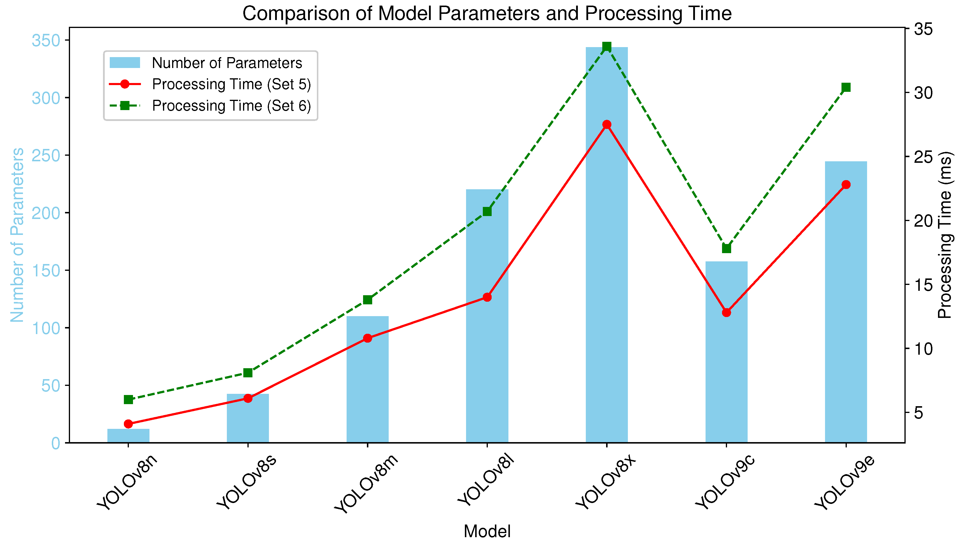
The number of parameters during inference for YOLOv8-seg (covering sizes from nano (n) to extra-large (x)) and YOLOv9-seg models (compact (c) and extended (e) variants) are summarized in

Table 7. Validation specifications for YOLOv8-seg and YOLOv9-seg models. n, s, m, l, x, c, and e indicate nano, small, medium, large, extra-large, compact, and extended models, respectively.

Model	Number of Parameters
YOLOv8n	3,258,259
YOLOv8s	11,779,987
YOLOv8m	27,222,963
YOLOv8l	45,912,659
YOLOv8x	71,721,619
YOLOv9c	27,625,299
YOLOv9e	59,682,451

.

2.9. Computational Environment and Reproducibility

All training and validation processes were conducted on a local workstation (Dell, Dell Canada Inc., Ontario, Canada) running Ubuntu 22.04.1 LTS, equipped with a 13th Gen Intel Core i9-13900K processor (24 cores, 32 threads, up to 5.5 GHz), 64 GB of RAM, and an NVIDIA GeForce RTX 4090 GPU with 24 GB of VRAM. The environment was managed using Conda and Python 3.11.9. Deep learning experiments were implemented using PyTorch 2.4.1 with CUDA 12.1.105 and cuDNN 9.1.0. We employed the official Ultralytics implementations of YOLOv8 and YOLOv9 (v 8.2.50) without internal modifications. Additional libraries included Torchvision 0.19.1, OpenCV 4.10.0.84, NumPy 1.26.4, and Pandas 2.2.3.

3. Results

The performance evaluation of YOLO segmentation models encompasses five key metrics—mask mAP50-95, Intersection over Union (IoU), Dice Coefficient, fragment spatial accuracy, False Positive count, and computational efficiency. Each metric provides distinct insights into model performance for automated tissue fragment analysis.

Models were evaluated on two test datasets containing identical cassettes captured at different resolutions; Set5 contains 100 images at 1MP resolution (1280 × 800 pixels), while Set6 contains 100 images at 5 MP resolution (2592 × 1944 pixels). To assess the overall model performance across different imaging conditions, we computed metrics on combined sets.

The mask mAP50-95 is calculated before the added post-processing phase for the YOLO outputs. The remaining metrics are calculated after the added post-processing phase. Each model configuration was trained with six random seeds to ensure statistical reliability.

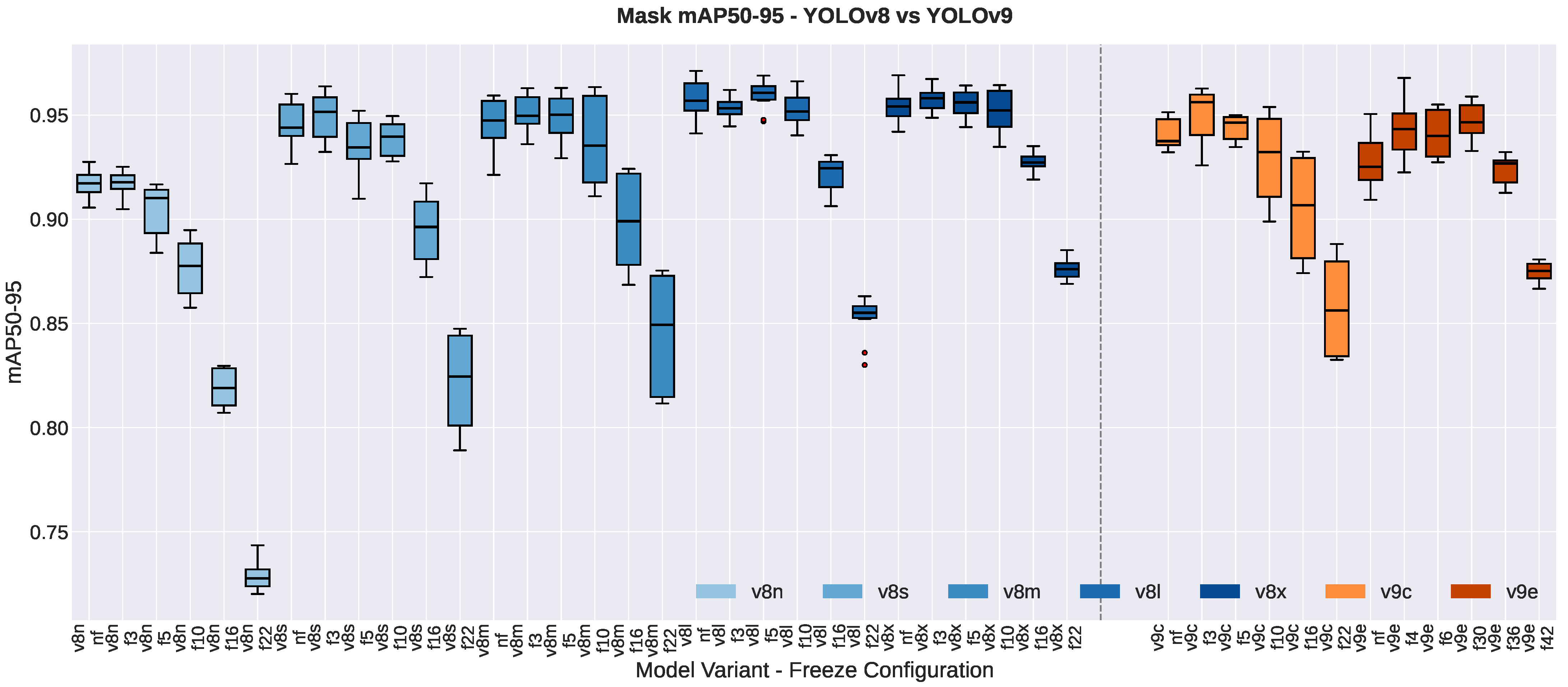
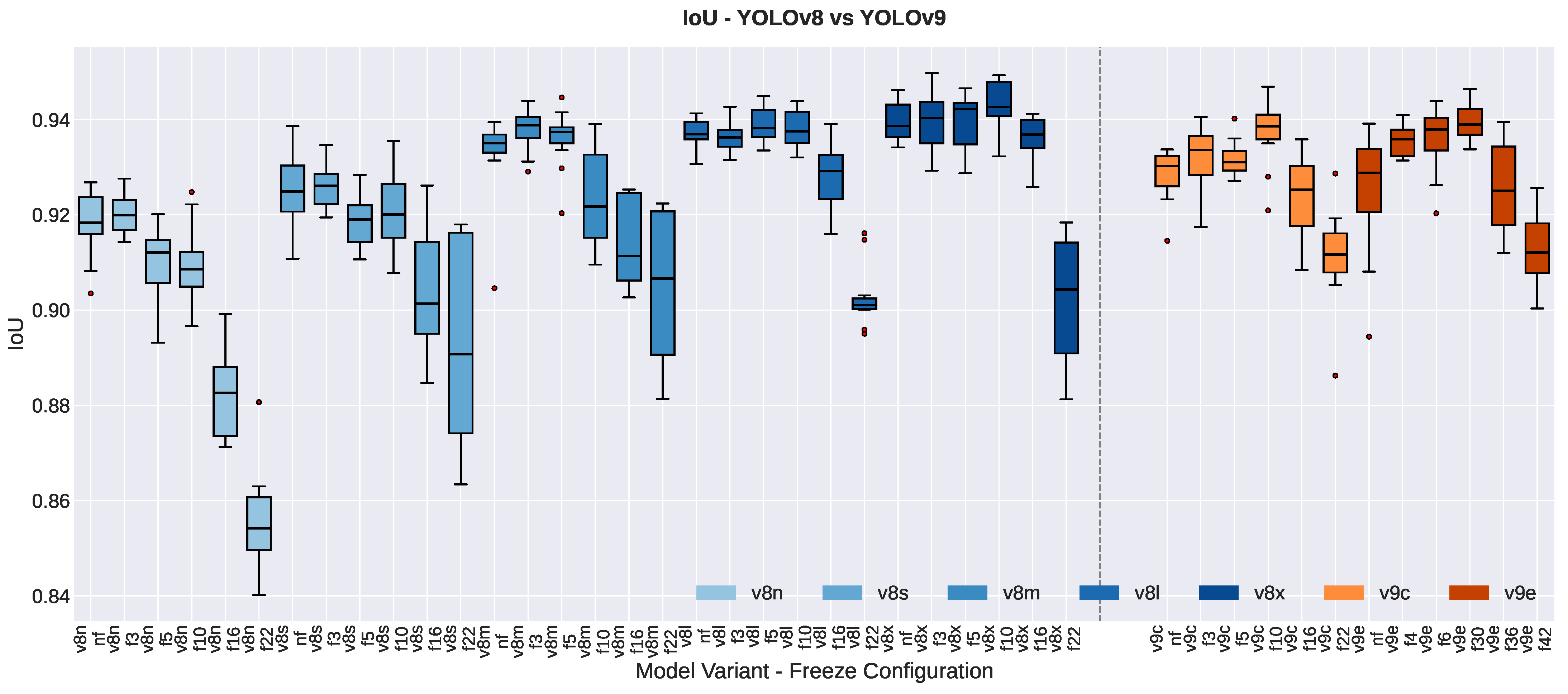
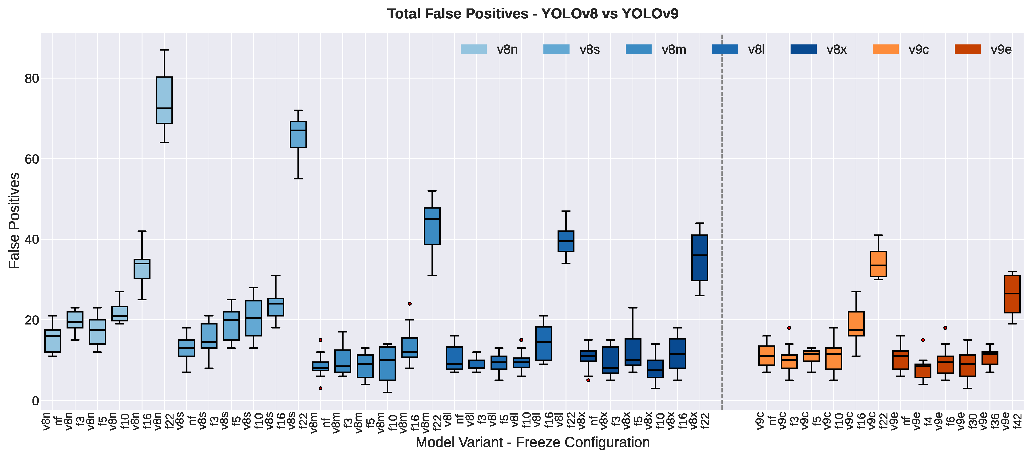
The performances of YOLOv8 and YOLOv9 variants under different layer-freezing strategies are depicted in Figure 8, Figure 9, Figure 10, Figure 11 and Figure 12, with each box plot showing the combined distribution across Sets 5 and 6 (detailed results in Tables S1 and S2).

Performance differences were evaluated using one-way ANOVA with Tukey’s HSD post hoc tests. Separate analyses were conducted to compare the baseline performance across models and freezing strategies within each model. Assumptions of normality (Shapiro–Wilk test) and homogeneity of variance (Levene’s test) were assessed prior to analyses. While some metrics showed violations, we proceeded with parametric analyses given ANOVA’s robustness with equal sample sizes (n = 6 per dataset; n = 12 combined) and confirmed findings through effect size measurements (${\omega }^2$). Statistical significance was set at 0.05, with results reported as mean ± standard deviation.

3.1. Impact of Model Size

The baseline performance evaluation (no freeze) assessed four key metrics for fragment segmentation quality—spatial accuracy, False Positive count, IoU, and Dice Coefficient. One-way ANOVA revealed significant differences among models for most metrics (detailed numerical results in Table S3).

3.1.1. False Positive Count

ANOVA showed significant differences in False Positive count (F(6,77) = 5.762, p < 0.001, ${\omega }^2$ = 0.254), with a large effect size. YOLOv8n exhibited the highest False Positive count (15 ± 3), which was significantly lower than all larger models including YOLOv8l (p = 0.005), YOLOv8x (p = 0.009), YOLOv9c (p = 0.046), and YOLOv9e (p = 0.004). In contrast, YOLOv8m demonstrated the best False Positive count (8 ± 3), significantly outperforming both YOLOv8n (p < 0.001) and YOLOv8s (p = 0.019).

3.1.2. Spatial Accuracy Improvements

When combining both datasets, ANOVA showed significant differences (F(6,77) = 2.554, p = 0.026, ${\omega }^2$ = 0.100), indicating a medium effect size. While the overall model comparison was significant, post hoc Tukey’s HSD tests revealed no significant pairwise differences after correction. The models ranked as follows: YOLOv8x (94.88 ± 1.02%) > YOLOv8l (94.84 ± 0.79%) > YOLOv8m (94.31 ± 2.00%) > YOLOv8s (93.87 ± 1.28%) ≈ YOLOv9c (93.87 ± 0.97%) > YOLOv8n (93.26 ± 0.85%) > YOLOv9e (93.09 ± 2.73%).

3.1.3. Segmentation Quality Metrics

IoU Performance: The combined dataset analysis revealed highly significant differences (F(6,77) = 10.777, p < 0.001, ${\omega }^2$ = 0.411), with a large effect size. Post hoc tests revealed overlapping performance groups—YOLOv8x (0.9392 ± 0.0041) achieved the highest performance in group ‘a’, while YOLOv8l (0.9371 ± 0.0031) and YOLOv8m (0.9328 ± 0.0093) formed an overlapping intermediate group ‘ab’. YOLOv9c (0.9284 ± 0.0056) occupied group ‘b’, YOLOv9e (0.9250 ± 0.0131) and YOLOv8s (0.9249 ± 0.0081) formed group ‘bc’, and YOLOv8n (0.9183 ± 0.0071) showed the lowest performance in group ‘c’. Notably, YOLOv8x significantly outperformed YOLOv8n (p < 0.001), YOLOv8s (p = 0.0005), YOLOv9c (p = 0.0182), and YOLOv9e (p = 0.0006).

Dice Coefficient: Similar patterns emerged for the Dice Coefficient (F(6,77) = 6.808, p < 0.001, ${\omega }^2$ = 0.293), with a large effect size. YOLOv8x (0.9643 ± 0.0036) achieved the highest performance in group ‘a’, significantly outperforming YOLOv8n (p < 0.001), YOLOv8s (p = 0.0024), and YOLOv9e (p = 0.0085). The overlapping group structure showed YOLOv8l (0.9620 ± 0.0018), YOLOv8m (0.9583 ± 0.0090), and YOLOv9c (0.9547 ± 0.0059) in group ‘ab’, while YOLOv9e (0.9525 ± 0.0141), YOLOv8s (0.9512 ± 0.0082), and YOLOv8n (0.9477 ± 0.0071) formed group ‘b’.

3.1.4. Resolution Effects

The model performance across resolutions was compared using paired t-tests, with models being paired by random seed to control for initialization variance. This paired design allowed for the isolation of resolution effects, while controlling for training randomness. Effect sizes were calculated using Cohen’s d for paired samples, with values of 0.2, 0.5, and 0.8 indicating small, medium, and large effects, respectively.

Paired t-tests comparing 1 MP (Val5) versus 5 MP (Val6) performance, as presented in

Table 8. Resolution effects on baseline performance. Paired t-tests comparing 1 MP (Val5) versus 5 MP (Val6) datasets.

Model	Metric	Val5 (1 MP)	Val6 (5 MP)	Difference	t-Stat	p-Value	Cohen’s d
	Spatial Accuracy (%)
YOLOv8n		93.39 ± 0.62	93.13 ± 1.07	−0.26	0.82	0.448	−0.34
YOLOv8s		94.00 ± 1.15	93.75 ± 1.50	−0.25	0.43	0.687	−0.17
YOLOv8m		94.78 ± 0.81	93.83 ± 2.76	−0.95	0.85	0.435	−0.35
YOLOv8l		94.88 ± 0.76	94.81 ± 0.88	−0.06	0.14	0.897	−0.06
YOLOv8x		94.44 ± 0.95	95.33 ± 0.94	+0.89	−1.21	0.279	0.50
YOLOv9c		93.63 ± 1.16	94.12 ± 0.77	+0.49	−0.82	0.449	0.34
YOLOv9e		91.86 ± 3.10	94.31 ± 1.79	+2.45	−1.59	0.173	0.65
	False Positive Count
YOLOv8n		18 ± 3	13 ± 2	−4.50	4.26	0.008 **	−1.74
YOLOv8s		13 ± 3	13 ± 3	−0.17	0.18	0.867	−0.07
YOLOv8m		10 ± 3	7 ± 2	−3.33	2.29	0.070	−0.94
YOLOv8l		11 ± 4	10 ± 3	−1.83	1.03	0.350	−0.42
YOLOv8x		13 ± 2	9 ± 3	−4.00	2.78	0.039 *	−1.14
YOLOv9c		12 ± 4	11 ± 3	−0.83	0.64	0.550	−0.26
YOLOv9e		12 ± 3	9 ± 3	−3.00	1.91	0.114	−0.78
	IoU
YOLOv8n		0.9205 ± 0.0052	0.9161 ± 0.0085	−0.0044	1.97	0.105	−0.81
YOLOv8s		0.9259 ± 0.0100	0.9238 ± 0.0064	−0.0022	0.64	0.548	−0.26
YOLOv8m		0.9367 ± 0.0030	0.9290 ± 0.0121	−0.0076	1.96	0.108	−0.80
YOLOv8l		0.9387 ± 0.0030	0.9354 ± 0.0024	−0.0033	6.19	0.002 **	−2.53
YOLOv8x		0.9423 ± 0.0029	0.9361 ± 0.0021	−0.0062	3.60	0.016 *	−1.47
YOLOv9c		0.9302 ± 0.0029	0.9265 ± 0.0072	−0.0037	1.03	0.349	−0.42
YOLOv9e		0.9210 ± 0.0172	0.9289 ± 0.0066	+0.0079	−1.22	0.275	0.50
	Dice Coefficient
YOLOv8n		0.9479 ± 0.0063	0.9475 ± 0.0084	−0.0004	0.20	0.850	−0.08
YOLOv8s		0.9507 ± 0.0107	0.9517 ± 0.0057	+0.0010	−0.31	0.769	0.13
YOLOv8m		0.9611 ± 0.0033	0.9554 ± 0.0121	−0.0057	1.55	0.182	−0.63
YOLOv8l		0.9629 ± 0.0018	0.9612 ± 0.0014	−0.0018	5.35	0.003 **	−2.18
YOLOv8x		0.9663 ± 0.0034	0.9623 ± 0.0027	−0.0040	1.77	0.137	−0.72
YOLOv9c		0.9557 ± 0.0039	0.9537 ± 0.0076	−0.0021	0.53	0.622	−0.21
YOLOv9e		0.9469 ± 0.0178	0.9580 ± 0.0066	+0.0111	−1.55	0.181	0.63

Note: Values are presented as mean ± standard deviation. For False Positive count, negative differences indicate improvement (fewer False Positives) at higher resolution. For IoU and Dice, negative differences indicate performance degradation at higher resolution. * p < 0.05, ** p < 0.01. Cohen’s d: 0.2 = small, 0.5 = medium, 0.8 = large effect.

, revealed limited resolution impacts. A significant degradation at higher resolutions was observed for YOLOv8l (IoU: −0.0033, p = 0.002, d = −2.53; Dice: −0.0018, p = 0.003, d = −2.18) and YOLOv8x (IoU: −0.0062, p = 0.016, d = −1.47). For False Positive control, YOLOv8n showed significant improvement at higher resolution (−4.50 false positives, p = 0.008, d = −1.74), as did YOLOv8x (−4.00, p = 0.039, d = −1.14).

3.2. Impact of Freezing Strategies

The freezing strategy analysis examined performance changes across different freeze levels for all model architectures. One-way ANOVA revealed significant effects across all models (p < 0.001), with effect sizes (${\omega }^2$) ranging from 0.386 to 0.974, indicating large practical significance (detailed numerical results in Tables S4–S7).

Small models demonstrated the highest freezing sensitivity, with no performance improvements at any freeze level. YOLOv8n (F(5,66) = 532.60, p < 0.001, ${\omega }^2$ = 0.974), with light freezing, showed no benefits at freeze3 (accuracy: −1.13%, p = 0.236) or freeze5 (accuracy: −0.61%, p = 0.829). Significant degradation began at freeze10 for spatial accuracy (−2.84%, p < 0.001) and False Positive count (+6.25, p = 0.017). Deep freezing at freeze16 caused severe degradation across all metrics (accuracy: −6.43%, p < 0.001; FP: +17.50, p < 0.001; IoU: −0.036, p < 0.001; Dice: −0.030, p < 0.001). Maximum freezing (freeze22) reduced the accuracy to 71.60% from 93.26% at baseline.

YOLOv8s (F(5,66) = 248.30, p < 0.001, ${\omega }^2$ = 0.945), with light freezing at freeze5, reported a significantly increased False Positive count (+6.25, p = 0.008) despite non-significant changes in other metrics. Freeze10 showed no significant degradation (accuracy: −0.85%, p = 0.574). A significant decline occurred at freeze16 (accuracy: −3.72%, p < 0.001; IoU: −0.021, p = 0.0006; Dice: −0.015, p = 0.015). Maximum freezing reduced the accuracy to 78.96% from 93.87%.

Small models showed no performance improvements from freezing at any level, with YOLOv8s showing significant degradation at freeze5 and YOLOv8n at freeze10.

Medium models demonstrated intermediate freezing tolerance with mixed responses to light freezing. YOLOv8m (F(5,66) = 183.28, p < 0.001, ${\omega }^2$ = 0.927) showed resilience through freeze10 with no significant changes in any metric (freeze3: accuracy +0.27%, p = 0.997; freeze10: accuracy −1.34%, p = 0.201). Significant degradation began at freeze16 (accuracy: −4.51%, p < 0.001; IoU: −0.019, p = 0.0005; Dice: −0.016, p = 0.001). Maximum freezing reduced the accuracy to 80.28%, with False Positives increasing to 43 from 8 (p < 0.001).

YOLOv9c (F(5,66) = 130.12, p < 0.001, ${\omega }^2$ = 0.900) demonstrated a significant accuracy improvement at freeze3 (+1.61%, p = 0.041) with non-significant positive trends in segmentation metrics. Freeze10 maintained a stable performance (accuracy: +0.50%, p = 0.935) while achieving significant improvements in IoU (+0.009, p = 0.041) and Dice (+0.0097, p = 0.008). Significant degradation occurred at freeze16 (accuracy: −3.00%, p < 0.001; FP: +7.08, p = 0.0003) while IoU remained relatively stable (−0.0042, p = 0.737).

YOLOv8m showed no significant changes through freeze10, with significant degradation beginning at freeze16. YOLOv9c demonstrated a significant accuracy improvement at freeze3 (p = 0.041), with other metrics showing non-significant positive trends, before significant degradation at freeze16.

Large models showed improvement trends with light freezing, though statistical significance varied. YOLOv8l (F(5,66) = 275.61, p < 0.001, ${\omega }^2$ = 0.950) showed consistent but non-significant improvements through freeze10. At freeze3, the accuracy increased by 0.64% (p = 0.841), with False Positives improving from 10 to 9 (p = 0.826). Freeze5 showed the best IoU (0.9391), though it was not significantly different from baseline. Significant degradation only occurred at freeze16 (accuracy: −4.57%, p < 0.001; IoU: −0.009, p = 0.0003).

YOLOv8x (F(5,66) = 107.88, p < 0.001, ${\omega }^2$ = 0.881) demonstrated substantial improvements but did not reach statistical significance. At freeze3, the accuracy improved by 0.84% (p = 0.840), with False Positives decreasing from 11 to 10 (p = 0.991). Freeze10 showed the highest absolute performance, with accuracy at 96.07% (+1.19%, p = 0.552) and IoU at 0.9430 (+0.004, p = 0.808). Remarkably, YOLOv8x is the only YOLOv8 model showing no significant degradation at freeze16 (accuracy: −1.96%, p = 0.076).

YOLOv9e (F(5,66) = 68.14, p < 0.001, ${\omega }^2$ = 0.823) exhibited the most remarkable improvement pattern with statistically significant enhancements at multiple freeze levels. At freeze4, significant improvements occurred in accuracy (+2.89%, p = 0.004) and IoU (+0.011, p = 0.026). Remarkably, significant improvements continued at freeze30—accuracy increased by 3.11% (p = 0.001), IoU by 0.015 (p = 0.0006), and Dice by 0.015 (p = 0.002). Even at freeze36, the performance remained stable (accuracy: −0.84%, p = 0.871; IoU: +0.0011, p = 0.999); degradation was only reported at freeze42.

YOLOv8l and YOLOv8x showed consistent but non-significant improvements through freeze10. YOLOv9e demonstrated significant improvements at freeze4 (accuracy and IoU) and freeze30 (accuracy, IoU, and Dice), maintaining benefits through freeze36 before degrading at freeze42.

3.3. Computational Configuration and Efficiency

All training and validation processes were conducted on a high-performance system equipped with a 13th Gen Intel Core i9-13900K processor (PassMark CPU score: 58,261), featuring 24 cores, 32 threads, and a maximum clock speed of 5.5 GHz, paired with an NVIDIA GeForce RTX 4090 with 24 GB of memory (PassMark G3D score: 38,430) and 64 GB of DDR5 RAM (PassMark Memory score: 3556). The edge computing platform utilizes a Raspberry Pi 5 Model B with a Cortex-A76 processor (PassMark CPU score: 2245, Memory score: 1356), which captures images locally and transmits them to the main system for segmentation processing.

This configuration demonstrates a computational performance ratio of 26:1 between the training/inference server and the edge platform, validating the necessity of our distributed architecture where computationally intensive segmentation tasks are performed on the server, while the Raspberry Pi handles image acquisition and result display. The memory bandwidth differential (43.9 GB/s vs. 9.1 GB/s) further justifies this architectural decision.

Training times with full parameter fine-tuning (no frozen layers) varied significantly based on model complexity: YOLOv8n completed training in 0.072 h (batch size = 13), YOLOv8x in 0.492 h (batch size = 2), and YOLOv9e in 0.618 h (batch size = 1). The inverse relationship between model size and feasible batch size reflects GPU memory constraints.

From Figure 13, it can be seen that processing times showed linear scaling with model parameters, providing predictable performance characteristics for deployment planning. Within the YOLOv8 family, YOLOv8n (3.3 M parameters) achieved the fastest inference, at 4.1 ms for Set5 and 6.0 ms for Set6 images. Processing times increased progressively from YOLOv8s (11.8 M parameters) at 7.2 ms/10.1 ms, YOLOv8m (27.2 M parameters) at 11.8 ms/15.2 ms, YOLOv8l (45.9 M parameters) at 18.5 ms/23.1 ms to YOLOv8x (71.7 M parameters), requiring 27.5 ms/33.6 ms for Set5/Set6, respectively. YOLOv9 models demonstrated a lower computational efficiency compared to similarly sized YOLOv8 variants. YOLOv9c (27.6 M parameters) required 14.2 ms/18.7 ms for Set5/Set6, which is approximately 20% slower than the comparable YOLOv8m. YOLOv9e (59.7 M parameters) needed 22.8 ms/30.4 ms, showing a similar inefficiency relative to its parameter count. Across all models, higher-resolution Set6 images required additional processing time.

3.4. Performance–Efficiency Trade-Offs

Optimal configuration selection depends on institutional priorities and constraints. For maximum accuracy with statistical validation, YOLOv9e with freeze30 achieves 96.20 ± 1.37% accuracy (p = 0.001) with 9 ± 4 False Positives, while YOLOv9e with freeze4 offers 95.98 ± 1.08% accuracy (p = 0.004) with better False Positive control (8 ± 3), both at 22.8–30.4 ms per image. YOLOv8x with freeze10 provides comparable performance at 96.07 ± 1.45% accuracy with 8 ± 3 False Positives, at 27.5–33.6 ms per image, achieving the best IoU (0.9430 ± 0.0049) and Dice (0.9691 ± 0.0041).

For laboratories requiring >95% accuracy with improved efficiency, YOLOv8l with freeze5 offers 95.85 ± 1.05% accuracy with 9 ± 3 False Positives at 18.5–23.1 ms per image—approximately 35% faster than YOLOv8x with minimal performance trade-off. This represents an optimal balance for clinical applications requiring high accuracy without maximum computational cost.

For routine screening prioritizing throughput and False Positive minimization, YOLOv8m without freezing provides 94.31 ± 2.00% accuracy with (8 ± 3) False Positive control at just 11.8–15.2 ms per image. Notably, this configuration matches YOLOv8x’s False Positive count while processing 2× faster, making it ideal for high-volume laboratories where False Positives incur significant review costs.

High-throughput environments should deploy YOLOv8s baseline (93.87 ± 1.28% accuracy, 13 ± 3 False Positives, 7.2–10.1 ms per image), processing 3-4× faster than YOLOv8x. Resource-constrained settings can utilize YOLOv8n baseline (93.26 ± 0.85% accuracy, 15 ± 3 False Positives, 4.1–6.0 ms per image) for edge deployment, achieving 6–7× speed improvement over YOLOv8x.

4. Discussion

With strategic layer-freezing, the YOLOv8 and YOLOv9 architectures achieve a remarkably similar performance despite their architectural differences. YOLOv8x + freeze10 reaches 96.07 ± 1.45% spatial accuracy with superior segmentation quality (IoU 0.9430 ± 0.0049, Dice 0.9691 ± 0.0041) and the best False Positive control (8 ± 3), while YOLOv9e + freeze30 achieves a slightly higher accuracy at 96.20 ± 1.37% (IoU 0.9397 ± 0.0039, Dice 0.9672 ± 0.0033) with 9 ± 4 False Positives. This convergence to >96% accuracy demonstrates that both architectures, when properly optimized, deliver a high performance for tissue fragment segmentation, regardless of their underlying complexity. However, their baseline performance reveals important differences. Without optimization, YOLOv8x achieved 94.88 ± 1.02% spatial accuracy compared to YOLOv9e’s 93.09 ± 2.73%—a 1.79% gap. Similarly, YOLOv8x reached a superior segmentation quality (IoU 0.9392 ± 0.0041) compared to YOLOv9e’s IoU 0.9250 ± 0.0131, with YOLOv8x maintaining 11 ± 3 False Positives compared to YOLOv9e’s 10 ± 3.

The effect of layer-freezing was particularly pronounced for YOLOv9 models, which showed statistically significant improvements. YOLOv9e improved from 93.09 ± 2.73% to 96.20 ± 1.37% (+3.11%, p = 0.001), while YOLOv9c gained 1.61%, reaching 95.49 ± 1.37% (p = 0.041) from baseline, at 93.87 ± 0.97%. YOLOv9e also demonstrated significant IoU improvements at both freeze4 (0.9356 ± 0.0034, +0.011, p = 0.026) and freeze30 (0.9397 ± 0.0039, +0.015, p = 0.0006), with False Positives improving to 8 ± 3 at freeze4. In contrast, the YOLOv8 models showed consistent but non-significant improvements. YOLOv8x improved from 94.88 ± 1.02% to 96.07 ± 1.45% (+1.19%, p = 0.552) with False Positives reducing from 11 ± 3 to 8 ± 3, while YOLOv8l showed modest gains from 94.84 ± 0.79% to 95.49 ± 0.88% (+0.64%, p = 0.841) with False Positives improving from 10 ± 3 to 9 ± 2.

This differential response suggests YOLOv8’s pre-trained features inherently align better with histology cassette patterns, achieving a strong baseline performance, while YOLOv9’s complex architecture requires careful preservation of early-layer features to prevent overfitting on our limited dataset. This phenomenon highlights how architectural sophistication designed for natural image benchmarks may require more careful optimization when applied to specialized medical domains with constrained training data.

Freezing tolerance varied significantly according to architecture and size. Small models (YOLOv8n, YOLOv8s) showed immediate degradation, with YOLOv8n significantly declining at freeze10 (from 93.26 ± 0.85% to 90.42 ± 1.14%, −2.84%, p < 0.001) with False Positives increasing from 15 ± 3 to 22 ± 2, and YOLOv8s showing increased False Positives at freeze5 (from 13 ± 3 to 19 ± 4, +6.25, p = 0.008). Medium models showed divergent patterns; YOLOv8m remained stable through freeze10 with no significant changes, while YOLOv9c achieved significant improvements at freeze3 (accuracy: 95.49 ± 1.37%, FP: 10 ± 4) and maintained IoU improvements at freeze10 (0.9374 ± 0.0072, p = 0.041) before degrading at freeze16 (FP increasing to 18 ± 5). Large models demonstrated the greatest flexibility, with YOLOv8x showing no significant degradation at freeze16 (92.92 ± 1.72%, p = 0.076, FP: 12 ± 4) and YOLOv9e maintaining performance through freeze30 with significant improvements (96.20 ± 1.37%, p = 0.001). This pattern aligns with larger models retaining representational capacity through deeper architectures. However, extensive freezing eventually limits adaptation, as seen in severe performance degradation at freeze22 for YOLOv8 models (e.g., YOLOv8l: 79.59 ± 1.41%, FP: 40 ± 3) and freeze42 for YOLOv9e (84.63 ± 2.44%, FP: 27 ± 5).

Resolution effects were minimal across most models without freezing. Paired t-tests comparing 1MP versus 5MP performance showed limited impact, though with notable exceptions. YOLOv8l showed significant degradation at higher resolutions for both IoU (from 0.9387 ± 0.0030 to 0.9354 ± 0.0024, −0.0033, p = 0.002) and Dice Coefficient (from 0.9629 ± 0.0018 to 0.9612 ± 0.0014, −0.0018, p = 0.003). YOLOv8x also showed significant IoU degradation (from 0.9423 ± 0.0029 to 0.9361 ± 0.0021, −0.0062, p = 0.016). For False Positive control, both YOLOv8n (from 18 ± 3 to 13 ± 2, −4.50, p = 0.008) and YOLOv8x (from 13 ± 2 to 9 ± 3, −4.00, p = 0.039) demonstrated significant improvement at higher resolution. YOLOv9e showed a +2.45% spatial accuracy improvement at 5MP (from 91.86 ± 3.10% to 94.31 ± 1.79%), though this was not statistically significant (p = 0.173). These results suggest that while both architectures maintain reasonable multi-scale feature extraction, larger models (YOLOv8l, YOLOv8x) showed more sensitivity to resolution changes in segmentation metrics, even as they improved in false positive control.

The optimal configuration identified was YOLOv8x at freeze10, achieving the best absolute IoU (0.9430 ± 0.0049) and Dice Coefficient (0.9691 ± 0.0041) with excellent False Positive control (8 ± 3), while YOLOv9e at freeze30 achieved the highest spatial accuracy (96.20 ± 1.37%) with statistically significant improvements across multiple metrics. Notably, YOLOv8m matched YOLOv8x’s False Positive count (8 ± 3). These findings demonstrate that strategic freezing can enhance performance beyond baseline capabilities, with the optimal freeze level being correlating with model size and architecture.

Figure 14 provides insights into model behavior at optimal configurations. Both YOLOv8x + freeze10 and YOLOv9e + freeze30 achieve a good performance, with a comparable spatial accuracy (96.07 ± 1.45% vs. 96.20 ± 1.37%) and the successful detection of both tissue fragments in this example. The proto layer visualizations reveal that both models show strong, concentrated activations precisely at fragment locations across all proto layers, demonstrating robust feature learning. The comparable performance demonstrates that both simpler (YOLOv8) and more complex (YOLOv9) architectures can effectively adapt to medical imaging tasks when appropriately configured.

Although newer YOLO versions (YOLOv10, YOLOv11, and YOLOv12) exist, we encountered specific limitations when evaluating them for our application. YOLOv10 currently lacks pre-trained segmentation weights, preventing its direct deployment for instance segmentation tasks. While we conducted a preliminary evaluation of the YOLOv11 segmentation models, YOLOv11x with freeze3 achieved a 95.46 ± 0.85% spatial accuracy, though with a notable False Positive rate (11 ± 3). This performance was competitive but did not surpass that of YOLOv9e at freeze30 (96.20 ± 1.37%, p = 0.001) or YOLOv8x at freeze10 (96.07 ± 1.45%). For YOLOv12, we observed significant memory constraints during training; for example, YOLOv12n required us to reduce the batch size from 13 (used in YOLOv8) to 4 when training without freezing layers, while larger YOLOv12 variants (m, l, x) could not be evaluated due to the memory constraints of our hardware. Future work will focus on a comprehensive multi-seed evaluation of YOLOv11 with hyperparameter optimization, as the preliminary results suggest these newer architectures may offer a competitive performance once properly validated and adapted to our domain-specific requirements and computational constraints.

5. Conclusions

This study highlights the critical role of gross examination in pathology and the challenges associated with manual tissue documentation, particularly in high-demand laboratory environments. Through the integration of advanced object detection and instance segmentation techniques, such as YOLOv8 and YOLOv9, we have demonstrated the potential for automation to enhance accuracy and efficiency in fragment identification and measurement.

The results highlight the importance of model architecture, dataset resolution, and training strategies in achieving optimal performance. Strategic layer-freezing proved particularly effective for large models, with YOLOv8x achieving the best overall performance through backbone freezing at freeze10, while YOLOv9e demonstrated significant improvements through backbone freezing at freeze30, effectively balancing pre-trained feature retention with tissue fragment-specific adaptation, particularly for smaller datasets.

By automating key steps in tissue documentation, the proposed framework offers a promising solution to streamline workflows, reduce human error, and improve traceability in pathology labs. Future work could focus on optimizing these models by expanding dataset diversity to improve generalizability and integrating this technology into existing laboratory workflows. Ultimately, this innovation represents a significant step toward modernizing gross examination practices and enhancing diagnostic precision in medical pathology.

Future research directions for this work include several promising avenues. First, we plan to expand our dataset with more diverse tissue types and cassette configurations to improve model generalization across different pathology laboratories. Second, we aim to investigate the other YOLO architectures as their segmentation capabilities mature, using architecture-specific optimization strategies to improve upon our preliminary results. Third, we plan to integrate voice command capabilities into the framework, enabling hands-free operation for technicians who need to maintain sterile conditions or have their hands occupied during the grossing process. This voice interface would allow users to control image capture, navigate results, and confirm measurements through spoken commands. Finally, we will conduct clinical validation studies in multiple pathology laboratories to assess the system’s impact on workflow efficiency, error reduction, and technician satisfaction in real-world settings. These advancements will further enhance the practical applicability and adoption of automated tissue documentation in clinical pathology.

References

1. Varma, M.; Collins, L.C.; Chetty, R.; Karamchandani, D.M.; Talia, K.; Dormer, J.; Vyas, M.; Conn, B.; Guzmán-Arocho, Y.D.; Jones, A.V.; et al. Macroscopic examination of pathology specimens: A critical reappraisal. J. Clin. Pathol. 2024, 77, 164–168. [Google Scholar] [CrossRef] [PubMed]
2. Cleary, A.S.; Lester, S.C. The Critical Role of Breast Specimen Gross Evaluation for Optimal Personalized Cancer Care. Surg. Pathol. Clin. 2022, 15, 121–132. [Google Scholar] [CrossRef] [PubMed]
3. Bell, W.C.; Young, E.S.; Billings, P.E.; Grizzle, W.E. The efficient operation of the surgical pathology gross room. Biotech. Histochem. 2008, 83, 71–82. [Google Scholar] [CrossRef] [PubMed]
4. Diepeveen, A. A Dilemma in Pathology: Overwork, Depression, and Burnout. Available online: https://lumeadigital.com/pathologists-are-overworked/ (accessed on 28 March 2025).
5. Vistapath. Vistapath Is Building the Next Generation of Pathology Labs: Optimize Your Grossing Workflows with Sentinel. Available online: https://www.vistapath.ai/sentinel/ (accessed on 28 March 2025).
6. Druffel, E.; Bridgeman, A.; Brandegee, K.; Bodell, A.; McClintock, D.; Garcia, J. Current State of Intra-/Interobserver Accuracy and Reproducibility in Tissue Biopsy Grossing and Comparison to an Automated Vision System. In Proceedings of the United States and Canada Association of Pathologists (USCAP) Annual Meeting, Baltimore, MD, USA, 23–28 March 2024. Poster #198. [Google Scholar]
7. Tissue-Tek AutoTEC® a120: An Automated Tissue Embedding System. Available online: https://www.sakuraus.com/Products/Embedding/AutoTEC-a120.html (accessed on 28 March 2025).
8. Greenlee, J.; Webster, S.; Gray, H.; von Bueren, E. Reducing Common Embedding Errors Through Automation: Manual Embedding Versus Automated Embedding Using the Tissue-Tek AutoTEC® a120 Automated Embedding System and the Tissue-Tek® Paraform® Sectionable Cassette System. In Proceedings of the National Society for Histotechnology (NSH) Annual Symposium, New Orleans, LA, USA, 20–25 September 2019; Sakura Finetek USA, Inc.: Torrance, CA, USA, 2019. Available online: https://www.sakuraus.com/getattachment/Products/Embedding/AutoTEC-a120/MPUB0012-Poster-NSH-2019-with-title-Reducing-common-embedding-errors-t.pdf?lang=en-US (accessed on 28 March 2025).
9. deBram Hart, M.; von Bueren, E.; Wander, B.; Fussner, M.; Scancich, C.; Reed, C.; Cockerell, C.J. Continuous Specimen Flow Changes Night Shifts to Day Shifts While Reducing Turn-Around-Time (TAT). In Proceedings of the National Society for Histotechnology (NSH) Annual Symposium, Washington, DC, USA, 28 August–2 September 2015; Cockerell Dermatopathology. Sakura Finetek USA, Inc.: Torrance, CA, USA, 2015. Available online: https://www.sakuraus.com/SakuraWebsite/media/Sakura-Document/Poster_1_-_AutoTEC_a120_-_NSH_2015.pdf (accessed on 28 March 2025).
10. Milestone Medical. eGROSS pro-x: Ergonomic Mobile Grossing Station. Product Brochure. 2019. Available online: https://www.milestonemedsrl.com/products/grossing-and-macro-digital/egross/ (accessed on 28 March 2025).
11. Roß, T.; Reinke, A.; Full, P.M.; Wagner, M.; Kenngott, H.; Apitz, M.; Hempe, H.; Mindroc-Filimon, D.; Scholz, P.; Tran, T.N.; et al. Comparative validation of multi-instance instrument segmentation in endoscopy: Results of the ROBUST-MIS 2019 challenge. Med. Image Anal. 2021, 70, 101920. [Google Scholar] [CrossRef] [PubMed]
12. Maier-Hein, L.; Wagner, M.; Ross, T.; Reinke, A.; Bodenstedt, S.; Full, P.M.; Hempe, H.; Mindroc-Filimon, D.; Scholz, P.; Tran, T.N.; et al. Heidelberg colorectal data set for surgical data science in the sensor operating room. Sci. Data 2021, 8, 101. [Google Scholar] [CrossRef] [PubMed]
13. Cheng, J.; Fu, B.; Ye, J.; Wang, G.; Li, T.; Wang, H.; Li, R.; Yao, H.; Cheng, J.; Li, J.; et al. Interactive medical image segmentation: A benchmark dataset and baseline. In Proceedings of the Computer Vision and Pattern Recognition Conference, Nashville, TN, USA, 10–17 June 2025; pp. 20841–20851. [Google Scholar]
14. Redmon, J.; Divvala, S.; Girshick, R.; Farhadi, A. You Only Look Once: Unified, Real-Time Object Detection. In Proceedings of the Conference on Computer Vision and Pattern Recognition, Las Vegas, NV, USA, 27–30 June 2016; pp. 779–788. [Google Scholar] [CrossRef]
15. Redmon, J.; Farhadi, A. YOLO9000: Better, Faster, Stronger. In Proceedings of the Conference on Computer Vision and Pattern Recognition, Honolulu, HI, USA, 21–26 July 2017; pp. 6517–6525. [Google Scholar] [CrossRef]
16. Redmon, J.; Farhadi, A. YOLOv3: An Incremental Improvement. arXiv 2018, arXiv:1804.02767. [Google Scholar] [CrossRef]
17. Bochkovskiy, A.; Wang, C.; Liao, H.M. YOLOv4: Optimal Speed and Accuracy of Object Detection. arXiv 2020, arXiv:2004.10934. [Google Scholar] [CrossRef]
18. Jocher, G. Ultralytics YOLOv5; Version 7.0; Ultralytics: Frederick, MD, USA, 2020; Available online: https://github.com/ultralytics/yolov5 (accessed on 28 March 2025).
19. Li, C.; Li, L.; Jiang, H.; Weng, K.; Geng, Y.; Li, L.; Ke, Z.; Li, Q.; Cheng, M.; Nie, W.; et al. YOLOv6: A Single-Stage Object Detection Framework for Industrial Applications. arXiv 2022, arXiv:2209.02976. [Google Scholar] [CrossRef]
20. Wang, C.Y.; Bochkovskiy, A.; Liao, H.Y.M. YOLOv7: Trainable Bag-of-Freebies Sets New State-of-the-Art for Real-Time Object Detectors. In Proceedings of the Conference on Computer Vision and Pattern Recognition, Vancouver, BC, Canada, 17–24 June 2023; pp. 7464–7475. [Google Scholar] [CrossRef]
21. Jocher, G.; Chaurasia, A.; Qiu, J. Ultralytics YOLOv8; Version 8.0.0; Ultralytics: Frederick, MD, USA, 2023; Available online: https://docs.ultralytics.com/models/yolov8/ (accessed on 28 March 2025).
22. Wang, C.Y.; Yeh, I.H.; Mark Liao, H.Y. YOLOv9: Learning What You Want to Learn Using Programmable Gradient Information. In Proceedings of the Computer Vision—ECCV 2024, Milan, Italy, 29 September–4 October 2024; Leonardis, A., Ricci, E., Roth, S., Russakovsky, O., Sattler, T., Varol, G., Eds.; Springer Nature: Cham, Switzerland, 2025; pp. 1–21. [Google Scholar]
23. Wang, A.; Chen, H.; Liu, L.; CHEN, K.; Lin, Z.; Han, J.; Ding, G. YOLOv10: Real-Time End-to-End Object Detection. In Proceedings of the International Conference on Neural Information Processing Systems, Vancouver, BC, Canada, 10–15 December 2024. [Google Scholar]
24. Jocher, G.; Qiu, J. Ultralytics YOLO11; Version 11.0.0; Ultralytics: Frederick, MD, USA, 2024; Available online: https://github.com/ultralytics/ultralytics (accessed on 28 March 2025).
25. Tian, Y.; Ye, Q.; Doermann, D. YOLOv12: Attention-Centric Real-Time Object Detectors. arXiv 2025, arXiv:2502.12524. [Google Scholar]
26. Ragab, M.G.; Abdulkadir, S.J.; Muneer, A.; Alqushaibi, A.; Sumiea, E.H.; Qureshi, R.; Al-Selwi, S.M.; Alhussian, H. A Comprehensive Systematic Review of YOLO for Medical Object Detection (2018 to 2023). IEEE Access 2024, 12, 57815–57836. [Google Scholar] [CrossRef]
27. Kumar, K.S.; Juliet, A.V. Microfluidic droplet detection for bio medical application using YOLO with COA based segmentation. Evol. Syst. 2024, 16, 21. [Google Scholar] [CrossRef]
28. AlSadhan, N.A.; Alamri, S.A.; Ben Ismail, M.M.; Bchir, O. Skin Cancer Recognition Using Unified Deep Convolutional Neural Networks. Cancers 2024, 16, 1246. [Google Scholar] [CrossRef] [PubMed]
29. Rong, R.; Sheng, H.; Jin, K.W.; Wu, F.; Luo, D.; Wen, Z.; Tang, C.; Yang, D.M.; Jia, L.; Amgad, M.; et al. A Deep Learning Approach for Histology-Based Nucleus Segmentation and Tumor Microenvironment Characterization. Mod. Pathol. 2023, 36. [Google Scholar] [CrossRef] [PubMed]
30. Zade, A.A.T.; Aziz, M.J.; Majedi, H.; Mirbagheri, A.; Ahmadian, A. Spatiotemporal analysis of speckle dynamics to track invisible needle in ultrasound sequences using convolutional neural networks: A phantom study. Int. J. Comput. Assist. Radiol. Surg. 2023, 18, 1373–1382. [Google Scholar] [CrossRef] [PubMed]
31. Tan, L.; Huangfu, T.; Wu, L.; Chen, W. Comparison of RetinaNet, SSD, and YOLO v3 for real-time pill identification. Bmc Med. Inform. Decis. Mak. 2021, 21, 324. [Google Scholar] [CrossRef] [PubMed]
32. Iriawan, N.; Pravitasari, A.A.; Nuraini, U.S.; Nirmalasari, N.I.; Azmi, T.; Nasrudin, M.; Fandisyah, A.F.; Fithriasari, K.; Purnami, S.W.; Irhamah; et al. YOLO-UNet Architecture for Detecting and Segmenting the Localized MRI Brain Tumor Image. Appl. Comput. Intell. Soft Comput. 2024, 2024, 3819801. [Google Scholar] [CrossRef]
33. Hossain, A.; Islam, M.T.; Almutairi, A.F. A deep learning model to classify and detect brain abnormalities in portable microwave based imaging system. Sci. Rep. 2022, 12, 6319. [Google Scholar] [CrossRef] [PubMed]
34. Almufareh, M.F.; Imran, M.; Khan, A.; Humayun, M.; Asim, M. Automated Brain Tumor Segmentation and Classification in MRI Using YOLO-Based Deep Learning. IEEE Access 2024, 12, 16189–16207. [Google Scholar] [CrossRef]
35. George, J.; Hemanth, T.S.; Raju, J.; Mattapallil, J.G.; Naveen, N. Dental Radiography Analysis and Diagnosis using YOLOv8. In Proceedings of the International Conference on Smart Computing and Communications (ICSCC), Kochi, India, 17–19 August 2023; pp. 102–107. [Google Scholar] [CrossRef]
36. Microsoft Corporation. OCR—Optical Character Recognition—Azure AI Services. Available online: https://learn.microsoft.com/fr-fr/azure/ai-services/computer-vision/overview-ocr (accessed on 28 April 2025).
37. Baraneedharan, P.; Kalaivani, S.; Vaishnavi, S.; Somasundaram, K. Revolutionizing healthcare: A review on cutting-edge innovations in Raspberry Pi-powered health monitoring sensors. Comput. Biol. Med. 2025, 190, 110109. [Google Scholar] [CrossRef] [PubMed]
38. Kirillov, A.; Mintun, E.; Ravi, N.; Mao, H.; Rolland, C.; Gustafson, L.; Xiao, T.; Whitehead, S.; Berg, A.C.; Lo, W.Y.; et al. Segment Anything. In Proceedings of the International Conference on Computer Vision, Paris, France, 2–6 October 2023; pp. 4015–4026. [Google Scholar]
39. Ultralytics. Brief Summary of YOLOv8 Model Structure. 2023. Available online: https://github.com/ultralytics/ultralytics/issues/189 (accessed on 24 July 2025).
40. Lin, T.Y.; Maire, M.; Belongie, S.; Bourdev, L.; Girshick, R.; Hays, J.; Perona, P.; Ramanan, D.; Zitnick, C.L.; Dollár, P. Microsoft COCO: Common Objects in Context. arXiv 2015, arXiv:1405.0312. [Google Scholar] [CrossRef]
Figure 1. Illustrated workflow of the histological tissue processing pipeline, from specimen reception to digital slide visualization. The sequence includes the following: (1) “Specimen Reception” in a labeled fixative container; (2) “Case Creation” and data entry into the laboratory information system; (3) “Gross Examination” and measurement of the specimen; (4) “Insertion” of dissected fragments into labeled cassettes; (5) “Automated Tissue Processing” through dehydration, clearing, and paraffin infiltration; (6) “Paraffin Embedding” of tissue fragments in molds; (7) “Microtomy” to section paraffin blocks into thin ribbons; (8) “Tissue Flattening” on a warm water bath and mounting of sections onto glass slides; (9) “Slide Staining” using an automated stainer; and (10) “Slide Scanning” for digital visualization and analysis.
Applsci 15 09276 g001
Figure 2. Workflow for automated tissue fragment segmentation and dimensions calculation.
Applsci 15 09276 g002
Figure 3. System architecture of the automated tissue fragment documentation platform. The Raspberry Pi acts as the central orchestrator, communicating via secure HTTPS connections with both Azure cloud services for OCR-based ID extraction and the private GPU server for YOLO segmentation. This distributed architecture enables efficient processing while maintaining local control of results.
Applsci 15 09276 g003
Figure 4. YOLOv8-seg architecture used for tissue fragment instance segmentation, adapted from [39] with modified input dimensions for cassette imaging and extended segmentation modules.
Applsci 15 09276 g004
Figure 5. YOLOv9e-seg architecture used for tissue fragment instance segmentation.
Applsci 15 09276 g005
Figure 6. Illustrated workflow of the histological tissue processing pipeline, from specimen reception to digital slide visualization. The red-framed section highlights the key steps (3 and 4) where the platform is integrated.
Applsci 15 09276 g006
Figure 7. Proposed platform for the automated capture, segmentation, and quantification of tissue fragments and biopsies. Subfigure (a) shows the physical imaging platform, with the red-highlighted screen area corresponding to the interface content in (b,c). (b) displays the interface before image acquisition, allowing the user to trigger the capture. (c) presents the segmentation results with the number of fragments, their dimensions, and individual color-coded labels.
Applsci 15 09276 g007
Figure 8. Comparison of mask mAP50-95 between YOLOv8 variants (n, s, m, l, x) and YOLOv9 variants (c, e) across progressive layer-freezing strategies. Box plots show the distribution of mAP values aggregated from validation Sets 5 and 6 across 6 seeds, with boxes representing quartiles, black lines indicating medians, whiskers extending to 1.5× interquartile range, and red dots showing outliers. The vertical dashed line separates YOLOv8 models (left) from YOLOv9 models (right). The freezing levels range from no freeze (nf) to freeze 22/42 for YOLOv8/YOLOv9, respectively.
Applsci 15 09276 g008
Figure 9. IoU comparison between YOLOv8 variants (n, s, m, l, x) and YOLOv9 variants (c, e) across progressive layer-freezing strategies. Box plots show the distribution of IoU values aggregated from validation Sets 5 and 6 across 6 seeds, with boxes representing quartiles, black lines indicating medians, whiskers extending to 1.5× interquartile range, and red dots showing outliers. The vertical dashed line separates YOLOv8 models (left) from YOLOv9 models (right). The freezing levels range from no freeze (nf) to freeze 22/42 for YOLOv8/YOLOv9, respectively.
Applsci 15 09276 g009
Figure 10. Dice Coefficient comparison between YOLOv8 variants (n, s, m, l, x) and YOLOv9 variants (c, e) across progressive layer-freezing strategies. Box plots show the distribution of Dice values aggregated from validation Sets 5 and 6 across 6 seeds, with boxes representing quartiles, black lines indicating medians, whiskers extending to 1.5× interquartile range, and red dots showing outliers. The vertical dashed line separates YOLOv8 models (left) from YOLOv9 models (right). The freezing levels range from no freeze (nf) to freeze 22/42 for YOLOv8/YOLOv9, respectively.
Applsci 15 09276 g010
Figure 11. Spatial accuracy comparison between YOLOv8 variants (n, s, m, l, x) and YOLOv9 variants (c, e) across progressive layer-freezing strategies. Box plots show the distribution of accuracy values aggregated from validation Sets 5 and 6 across 6 seeds, with boxes representing quartiles, black lines indicating medians, whiskers extending to 1.5× interquartile range, and red dots showing outliers. The vertical dashed line separates YOLOv8 models (left) from YOLOv9 models (right). The freezing levels range from no freeze (nf) to freeze 22/42 for YOLOv8/YOLOv9, respectively.
Applsci 15 09276 g011
Figure 12. False Positive comparison between YOLOv8 variants (n, s, m, l, x) and YOLOv9 variants (c, e) across progressive layer-freezing strategies. Box plots show the distribution of False Positive values aggregated from validation Sets 5 and 6 across 6 seeds, with boxes representing quartiles, black lines indicating medians, whiskers extending to 1.5× interquartile range, and red dots showing outliers. The vertical dashed line separates YOLOv8 models (left) from YOLOv9 models (right). The freezing levels range from no freeze (nf) to freeze 22/42 for YOLOv8/YOLOv9, respectively.
Applsci 15 09276 g012
Figure 13. Comparison of YOLO segmentation models based on the number of parameters and processing time. The blue bars represent the number of parameters, while the red and green lines indicate the processing time per image for Sets 5 and 6, respectively.
Applsci 15 09276 g013
Figure 14. Comparison of proto layer activations between the YOLOv8x + freeze10 and YOLOv9e + freeze30 models at optimal configurations. The top row shows YOLOv8x successfully segmenting both tissue fragments. The bottom row shows YOLOv9e also successfully segmenting both fragments.
Applsci 15 09276 g014