An Improved TCN-BiGRU Architecture with Dual Attention Mechanisms for Spatiotemporal Simulation Systems: Application to Air Pollution Prediction

Abstract

Long-term and accurate prediction of air pollutant concentrations can serve as a foundation for air pollution warning and prevention, which is crucial for social development and human health. In this study, we provide a model for predicting the concentration of air pollutants based on big data spatiotemporal correlation analysis and deep learning methods. Based on an improved temporal convolutional network (TCN) and a bi-directional gated recurrent unit (BiGRU) as the fundamental architecture, the model adds two attention mechanisms to improve performance: Squeeze and Excitation Networks (SENet) and Convolutional Block Attention Module (CBAM). The improved TCN moves the residual connection layer to the network’s front end as a preprocessing procedure, improving the model’s performance and operating efficiency, particularly for big data jobs like air pollution concentration prediction. The use of SENet improves the model’s comprehension and extraction of long-term dependent features from pollutants and meteorological data. The incorporation of CBAM enhances the model’s perception ability towards key local regions through an attention mechanism in the spatial dimension of the feature map. The TCN-SENet-BiGRU-CBAM model successfully realizes the prediction of air pollutant concentrations by extracting the spatiotemporal features of the data. Compared with previous advanced deep learning models, the model has higher prediction accuracy and generalization ability. The model is suitable for prediction tasks from 1 to 12 h in the future, with root mean square error (RMSE) and mean absolute error (MAE) ranging from 5.309~14.043 and 3.507~9.200, respectively.

1. Introduction

Urbanization and industrialization have fueled economic growth in recent decades, but they have also resulted in a growing number of air pollution issues [1]. The Air Pollution Prevention and Control Action Plan (APPCAP) is one of the policies the state has implemented since 2013 to address the issue of air pollution, and an increasing number of people are deeply concerned about the sustainable and healthy development of the human environment in the future [2]. The WHO (World Health Organization) has determined that PM₂.₅, out of all the air pollutants, poses the greatest risk to human health since it causes a number of severe illnesses, including lung cancer and cardiovascular disease [3,4]. A precise PM₂.₅ concentration prediction can provide citizens and the government early notice so they can take preventative action. Thus, it is indisputable that achieving a long-term, accurate prediction of PM₂.₅ concentrations is crucial and a critical step in advancing society’s sustainable growth and creating a more positive vision of peaceful coexistence between humans and the natural world [5].

Data on the concentrations of air pollutants are shown as time series. Prediction methods to solve this problem of predicting air pollutant concentrations have evolved through three stages: statistical techniques based on meteorological principles, simple machine learning methods, and deep learning methods that have drawn the attention of numerous researchers in recent years [6]. Statistical methods often abstract complex mathematical physical equation models for prediction through atmospheric dynamics and chemical reactions [7]. The two most popular prediction techniques in statistics are multiple linear regression models [8] and Bayesian statistical models [9]. However, these prediction models usually assume ideal conditions, which makes them unsuitable for the complex and nonlinear challenges encountered in real-world applications. Furthermore, statistical models are ineffective at making predictions and require a lot of calculations in mathematics [10]. Therefore, in order to increase prediction accuracy and efficiency and adapt to real prediction situations, better methodologies are required for the prediction of air pollutant concentrations.

The second prediction method is a straightforward machine learning method that uses historical data analysis, pattern recognition, and manually operated feature engineering to estimate air pollution concentrations. Common machine learning methods include Decision Trees [11], k-means [12] and SVM [13]. In a recent study, Yang et al. [14] suggested using the Bootstrap-XGBoost model in conjunction with a resampling technique to forecast the AQI values of Xi’an over the course of the following 15 days. The study discovered that the model had a strong prediction impact. Zheng et al. [15] proposed 16 distinct integrated learning methods using logistic regression (LR), Catboost, random forest (RF), and other individual learners to be combined. Comparison experiments demonstrated that the performance of integrated learning models is typically superior to that of individual machine learning models. In real-world applications, machine learning methods outperform traditional statistical methods in resolving the nonlinear air pollution concentration predict problem. However, when dealing with more complicated nonlinear interactions and larger datasets, machine learning methods continue to fall short. Moreover, the majority of machine learning methods depend on human feature engineering to extract useful features from the data, which results in poor generalization ability for the machine learning models [16].

Deep learning methods have gained popularity in a number of domains because of their significant benefits in terms of nonlinear modeling and data processing power. In time series prediction issues, deep learning methods have proven to be highly effective, particularly for air pollution concentration prediction [17]. Ragab et al. [18] proposed a one-dimensional deep convolutional neural network (1D-CNN) optimized by exponential adaptive gradient (EAG), and showed that 1D-CNN can effectively predict the air pollution index (API). Chang et al. [19] aggregated three LSTM models into a single prediction model called ALSTM, which effectively improves the prediction accuracy compared with SVM, GBTR and other models. Gated Recurrent Unit (GRU) is a simplified version of LSTM, which is structurally optimized to enable it to extract timing information more efficiently. Similarly, temporal convolutional networks (TCNs) are variants of CNNs and are specifically used for time-series modeling problems. Saif-ul-Allah et al. [20] combined the model planar projection data analysis method (PMP) with GRUs to build a prediction model, and Samal et al. [21] built a multi-output temporal convolutional network auto encoder model (MO-TCNA), both deep learning models achieved good prediction results in the task of predicting air pollutant concentrations. In big data problems, deep learning models typically perform better than statistical models and basic machine learning models. However, when working with spatiotemporal large data that is rich in long-term and spatial features, deep learning models which only have a single structure also have drawbacks and perform badly [22].

Hybrid deep learning models can attain a greater performance ceiling by combining the benefits of several single deep learning models. In spatiotemporal big data training problems, hybrid deep learning models have surfaced in recent years. In order to extract spatiotemporal features from air quality data, Zhu et al. [23] developed a hybrid model named APSO-CNN-Bi-LSTM, which successfully combines CNN for spatial features and LSTM for temporal features. Faraji et al. [24] developed a 3D CNN-GRU combined model, which has a better application prospect for spatiotemporal large datasets because it can identify long-term temporal dependence in air pollutant data, according to experiments. Zhang et al. [25] also built an RCL-Learning hybrid deep learning model that performed well in a variety of prediction tasks by using the spatiotemporal feature extraction of pollutants and meteorological data as an entry point. The RCL-Learning model is a combination of the Convolutional Long Short-Term Memory Network (ConvLSTM) and the Residual Network (ResNet). It offers academics a novel research idea by concentrating on the temporal and spatial correlation of feature sequences.

Additionally, a growing number of academics are becoming interested in the application of attention mechanisms to enhance the performance and accuracy of deep learning models. Chen et al. [26] proposed a spatio-temporal attention mechanism (STA) enhanced prediction model called STA-ResConvLSTM. Experiments demonstrate that this attention mechanism can improve the model’s perception of spatio-temporal distribution features, thereby increasing prediction accuracy. Li et al. [27] proposed a new hybrid model CBAM-CNN-Bi LSTM by using the convolutional block attention module (CBAM) to extract the spatial distribution features of PM₂.₅. The ability of the CBAM attention mechanism to adaptively modify the feature weights greatly aids in increasing prediction accuracy. In summary, the current deep learning-based models for predicting the concentration of air pollutants face the following challenges: (1) the models become more complex as the prediction task grows, which results in issues with low operational efficiency and high overhead; (2) the models struggle to extract spatiotemporal features from the data. These are the challenges encountered when improving the prediction performance of the model.

Concluding the discussion above, the efficiency of air pollutant concentration prediction is linked to the extraction of spatiotemporal features. To address this issue and increase prediction accuracy, we suggest a new hybrid deep learning prediction model called TCN-SENet-BiGRU-CBAM. The improved time convolution network (TCN) and bi-directional gated recurrent unit (BiGRU) serve as its backbone, and it incorporates the two attention mechanisms of SENet and CBAM. The following is a summary of this work’s novelty and primary contributions.

(1)

A method to build data sets that is based on spatiotemporal correlation analysis. The selection of input features makes the dataset creation more rational and scientific by taking into account not only meteorological conditions and air pollutants in the forecast area, but also air pollutants that have a high connection in other cities outside the prediction area;

(2)

Improvement of the traditional TCN network: the residual connection layer in the network is moved forward and replaced by a preprocessing operation. By processing the residual connection beforehand during model initialization, the overhead at runtime is decreased, the model’s performance and operation efficiency are increased, and the need to repeatedly verify that the number of channels is constant is avoided;

(3)

The channel attention mechanism SENet is utilized to effectively extract the long-term dependent features of pollutants and meteorological data after the TCN layer is introduced. SENet can dynamically learn the dependencies between channels, select and enhance the output of TCN, so as to better capture the long-term dependencies;

(4)

Introducing the hybrid attention mechanism CBAM. The spatial attention module of CBAM operates on the spatial dimension of the feature map, assisting the model in focusing on more discriminative local regions within the output sequence of BiGRU.

The TCN-SENet-BiGRU-CBAM model can recognize patterns of long-term spatial and temporal change and realize the prediction of air pollutant concentrations. Experiments conducted on the dataset demonstrate that the suggested model outperforms other sophisticated deep learning prediction models in terms of prediction accuracy and performance.

2. Study Area and Dataset Analysis

2.1. Study Area

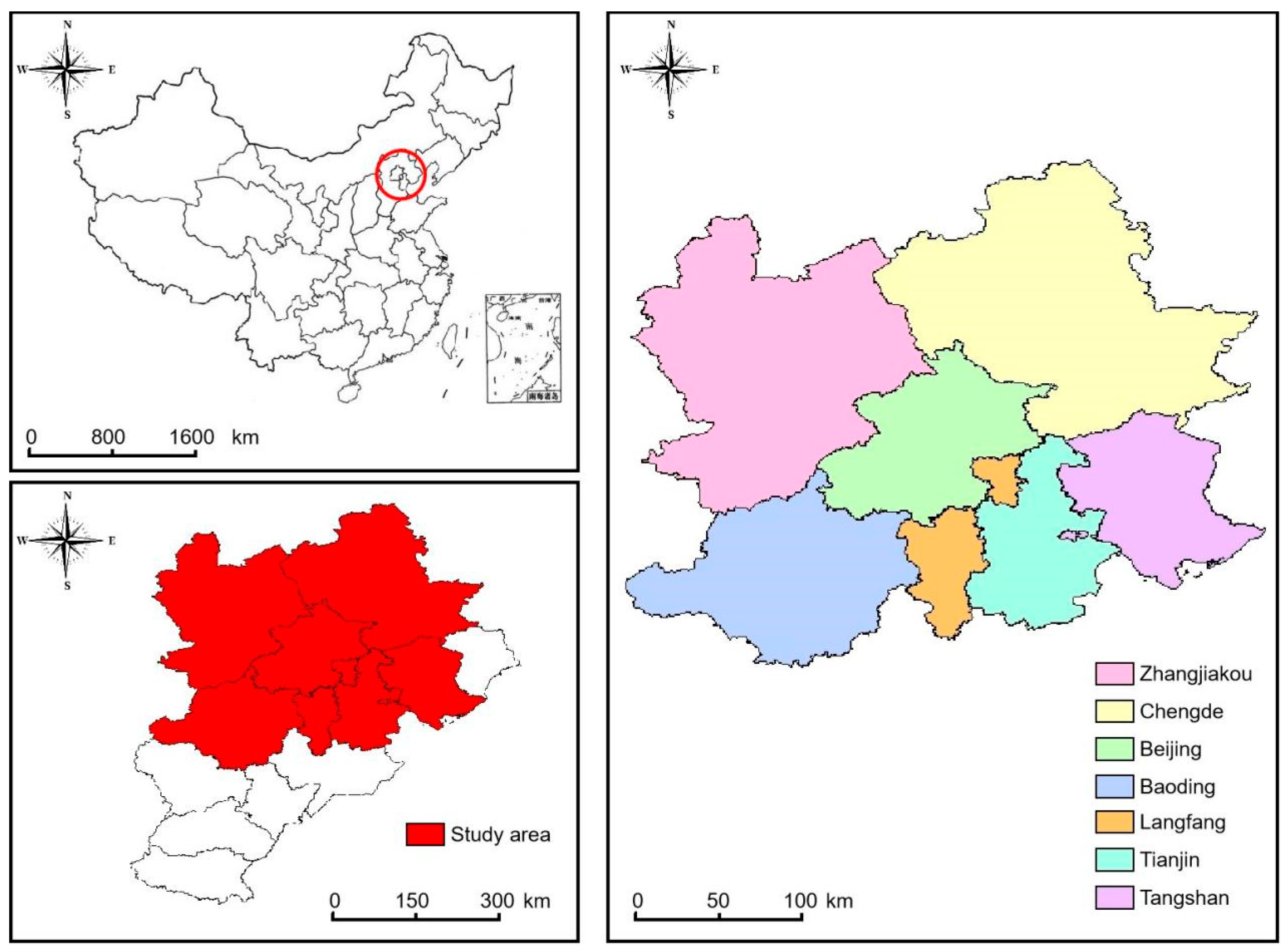
The study area of this paper is centered on Beijing, with the six neighboring cities (Tianjin, Langfang, Baoding, Zhangjiakou, Chengde, and Tangshan) supplemented to form the study area. Figure 1 shows the geographical distribution of the study area. Because the neighboring regions share similar geographic features, meteorological conditions, and atmospheric circulation patterns, pollutants can spread in the air and affect the surrounding neighboring regions [28]. The Beijing Tianjin Hebei metropolitan area in China is characterized by rapid economic growth, and Beijing, as the core city of the region, bears a great responsibility to drive the economic development of the region and the entire nation. However, Beijing’s air quality, particularly the concentration of PM₂.₅, typically varies between 35 and 80 µg/m³, which is much higher than the World Health Organization’s (WHO) recommended health threshold of 10 µg/m³ [29]. Therefore, forecasting Beijing’s PM₂.₅ concentration with accuracy is crucial. We primarily forecast Beijing’s PM₂.₅ concentration; the input features will also include the pollutants and meteorological data with high correlation in the other six cities.

2.2. Data Description

Hour-by-hour air pollutant and meteorological data from 1 January 2022, to 29 August 2024 in seven cities are used in the experiments to ensure the timeliness and accuracy of the study, taking into account the specific impact of virus transmission on the concentration and distribution of air pollutants in the pre-epidemic period.

Table 1. Statistical information of Beijing.

Factor		Max	Min	Mean
Air pollutants	$\mathrm{AQI}$ (µg/m3)	500.0	7.0	60.07
	${\mathrm{PM}}_{2.5}$ (µg/m3)	439.0	1.0	32.36
	${\mathrm{PM}}_{2.5} \_24 \mathrm{h}$ (µg/m3)	184.0	1.0	32.36
	${\mathrm{PM}}_{10}$ (µg/m3)	1667.0	2.0	64.33
	${\mathrm{PM}}_{10} \_24 \mathrm{h}$ (µg/m3)	691.0	3.0	64.33
	${\mathrm{SO}}_2$ (µg/m3)	18.0	1.0	2.85
	${\mathrm{SO}}_2 \_24 \mathrm{h}$ (µg/m3)	9.0	2.0	2.86
	${\mathrm{NO}}_2$ (µg/m3)	100.0	2.0	23.75
	${\mathrm{NO}}_2 \_24 \mathrm{h}$ (µg/m3)	79.0	2.0	23.77
	${\mathrm{O}}_3$ (µg/m3)	322.0	2.0	69.26
	${\mathrm{O}}_3 \_8 \mathrm{h}$ (µg/m3)	411.0	1.0	66.94
	CO (mg/m3)	2.03	0.11	0.49
	$\mathrm{CO} \_24 \mathrm{h}$ (mg/m3)	1.76	0.12	0.49
Meteorological phenomena	Temperature (℃)	40.6	−16.5	14.49
	Surface pressure (hPa)	1041.8	984.3	1011.79
	Relative humidity (%)	100.0	6.0	52.43
	Instantaneous wind direction (°)	360.0	0.0	160.80
	Instantaneous wind speed (m/s)	18.1	0.0	2.61
	1-hour maximum wind speed (m/s)	24.2	0.0	4.29
	1-hour precipitation (mm)	53.8	0.0	0.09
	10 min average visibility (km)	30.0	0.334	16.16

provides a comprehensive description of the data details by listing Beijing’s air pollution and meteorological statistics. We choose 13 indicators of air pollutants and 8 meteorological data (PM₂.₅_24 h shows the average PM₂.₅ concentration over the last 24 h). The air pollutant data comes from the shared data website (https://quotsoft.net/air/ (accessed on 1 October 2024)), while the meteorological data comes from the open meteorology website (https://openweathermap.org/ (accessed on 1 October 2024)).

2.3. Data Preprocessing

Preprocessing was done on air pollution and meteorological data from seven cities. To start, in order to simplify the model input, the average value of the related factor at each monitoring station was used for each city. Outliers were handled as missing values, as in the case of data with negative pollutant concentrations. Since less than 2% of each city’s data was missing, linear interpolation was then used to fill in the gaps. Lastly, to improve the model performance, the data were min-max normalized to fit the conventional normal distribution in order to remove the effect of dimension [30]. Following preprocessing, the train set consisted of 80% of the data, whereas the test set consisted of 20%.

2.4. Research on Data Characteristics

2.4.1. Characteristics of Time Dimension

Beijing’s air pollution and meteorological data from 1 January 2022 to 29 August 2024, were chosen in order to analyze their features in the temporal dimension.

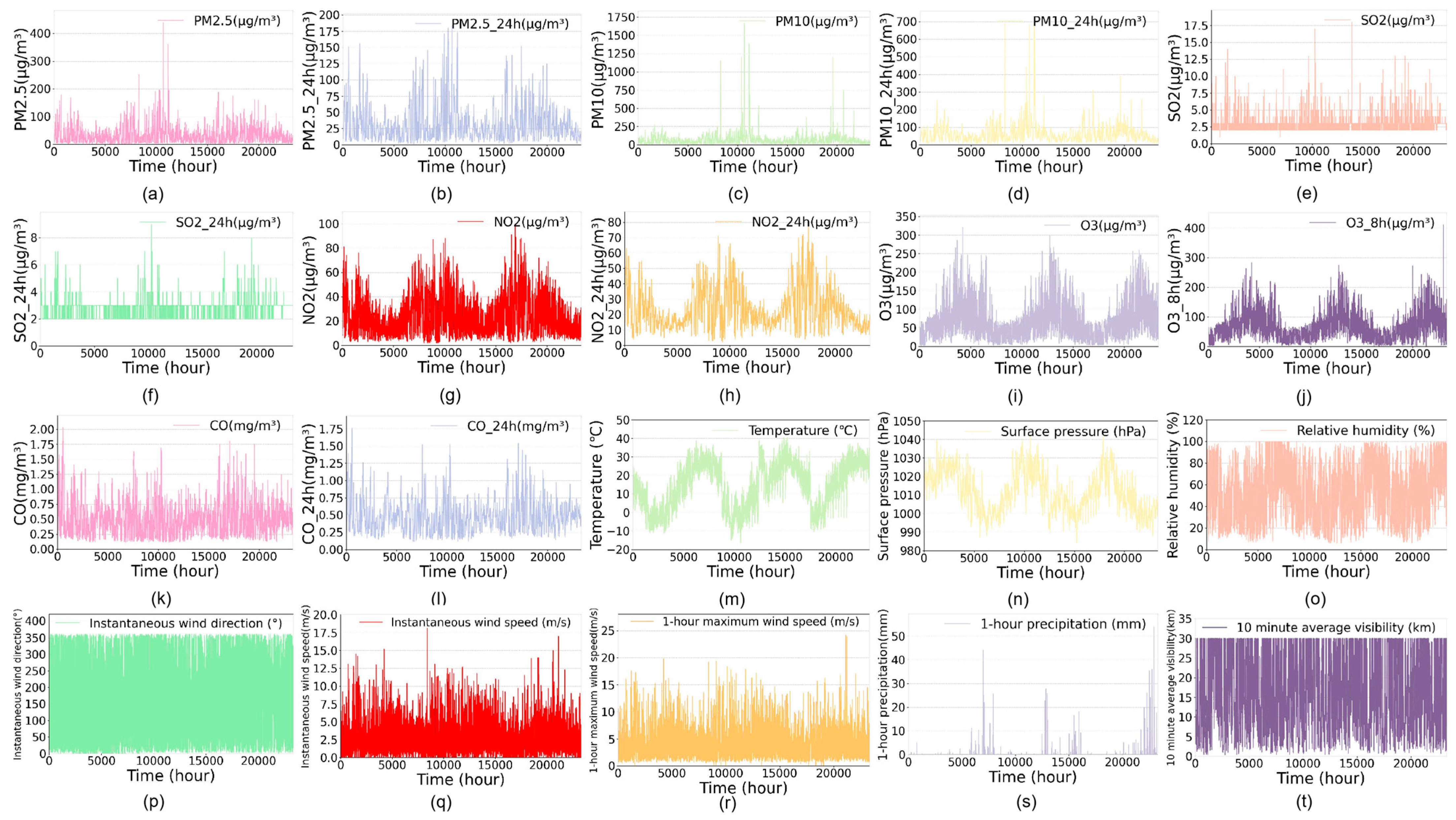
Figure 2 displays the time series plots of air pollutant and meteorological data, illustrating how each factor changed from 2022 to 2024. Figure 2 shows that the trends of the various air pollutants—PM₂.₅, PM₁₀, SO₂, and NO₂—over time are substantially the same, as are the times when local peaks and troughs take place. While the time-dependent trends of temperature and surface pressure are essentially opposite, the time-dependent trends of several meteorological parameters, such as temperature and relative humidity, instantaneous wind speed, and 1-hour maximum wind speed, are roughly the same. This indicates that there is an implicit relationship—that is, a time dependency—between meteorology and time as well as between air pollution and time. Thus, the time dependency of PM₂.₅ and the time dependency of other factors must be taken into account for PM₂.₅ prediction [31], and the dataset’s time span and sliding window length setting are especially crucial.

Additionally, Figure 2 illustrates the relationships that exist between air pollutants, meteorology, and air pollutants and meteorology. Among air pollutants, NO₂ from industrial and vehicle emissions and SO₂ from burning fossil fuels both contribute to the creation of PM₂.₅ through atmospheric chemical processes. Moreover, PM₂.₅ is a component of PM₁₀, which is influenced by PM₁₀ concentrations. Among meteorology, when temperatures rise, the air’s water vapor concentration rises as well, increasing relative humidity at the same time that surface pressure falls. Similar relationships between air pollutants and meteorology are demonstrated. For instance, when temperature reaches a local peak, the intensity of photochemical reactions in the atmosphere rises, resulting in a local peak in PM₂.₅ concentration; when 1-hour precipitation and instantaneous wind speed increase, atmospheric particles undergo aggregation, deposition, and dilution, causing a decrease in PM₂.₅ concentration. Therefore, we included both air pollutants and meteorological data as inputs to the model, taking into account the correlations and interactions among the elements.

2.4.2. Characteristics of Spatial Dimension

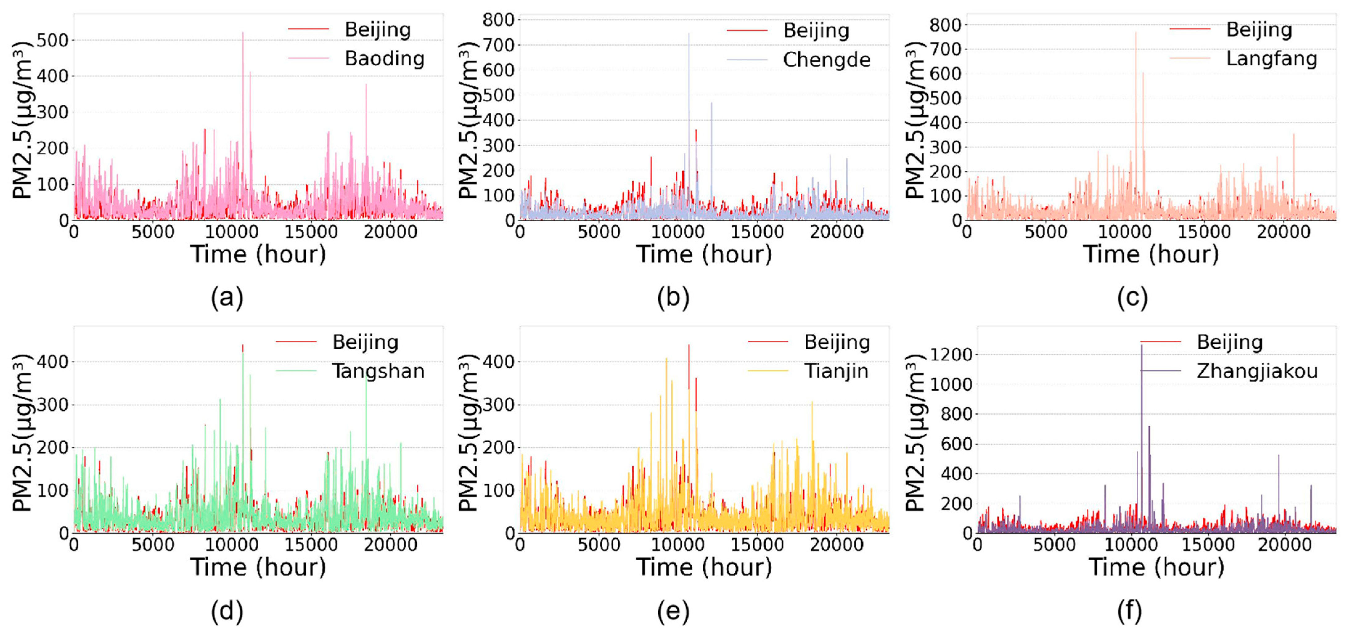
Spatial dimension characteristics must be taken into account when predicting PM₂.₅ concentrations in Beijing. The time trends of changes in PM₂.₅ concentrations in Beijing and six nearby cities were presented (Figure 3). Additionally, the Pearson correlation coefficients between each air pollutant in the six cities and Beijing PM₂.₅ were computed. The correlation coefficients between Beijing PM₂.₅ and air pollutants in other cities decrease as the distance between those cities and Beijing increases. Furthermore, among the six cities’ air pollutants, the correlation coefficients between Beijing PM₂.₅ and the corresponding cities’ PM₂.₅ are generally higher than those between other air pollutants. These findings are supported by Figure 3 and

Table 2. Pearson correlation between PM₂.₅ in Beijing and various pollutants in surrounding cities.

City Group	$\mathbf{AQI}$	${\mathbf{PM}}_{2.5}$	${\mathbf{PM}}_{10}$	${\mathbf{SO}}_2$	${\mathbf{NO}}_2$	${\mathbf{O}}_3$	CO
Beijing and Baoding	0.655	0.719	0.551	0.296	0.350	−0.124	0.514
Beijing and Chengde	0.612	0.763	0.456	0.185	0.497	−0.088	0.564
Beijing and Langfang	0.745	0.844	0.610	0.300	0.433	−0.138	0.625
Beijing and Tangshan	0.619	0.700	0.521	0.338	0.430	−0.118	0.423
Beijing and Tianjin	0.651	0.713	0.605	0.318	0.400	−0.123	0.523
Beijing and Zhangjiakou	0.457	0.513	0.268	0.273	0.450	−0.065	0.468

. This implies that there is a distance effect and spatial correlation among air pollutants [32]. Therefore, in order to introduce geographical spatial correlation information, we must include data on other urban air pollutants. In order to simplify the model’s inputs, we used PM₂.₅ in Langfang, which has a correlation value higher than 0.8 indicating a high positive correlation, as the model’s input feature.

Through the above-described time and spatial dimensions of the dataset analysis, we have identified the input content of the prediction model to guarantee the efficacy and scientificity of the prediction process. Our research will also concentrate on the extraction method of the spatiotemporal features that were revealed throughout the data set’s analysis process when we were designing the model.

3. Methodology

3.1. The Framework of the Proposed Prediction System

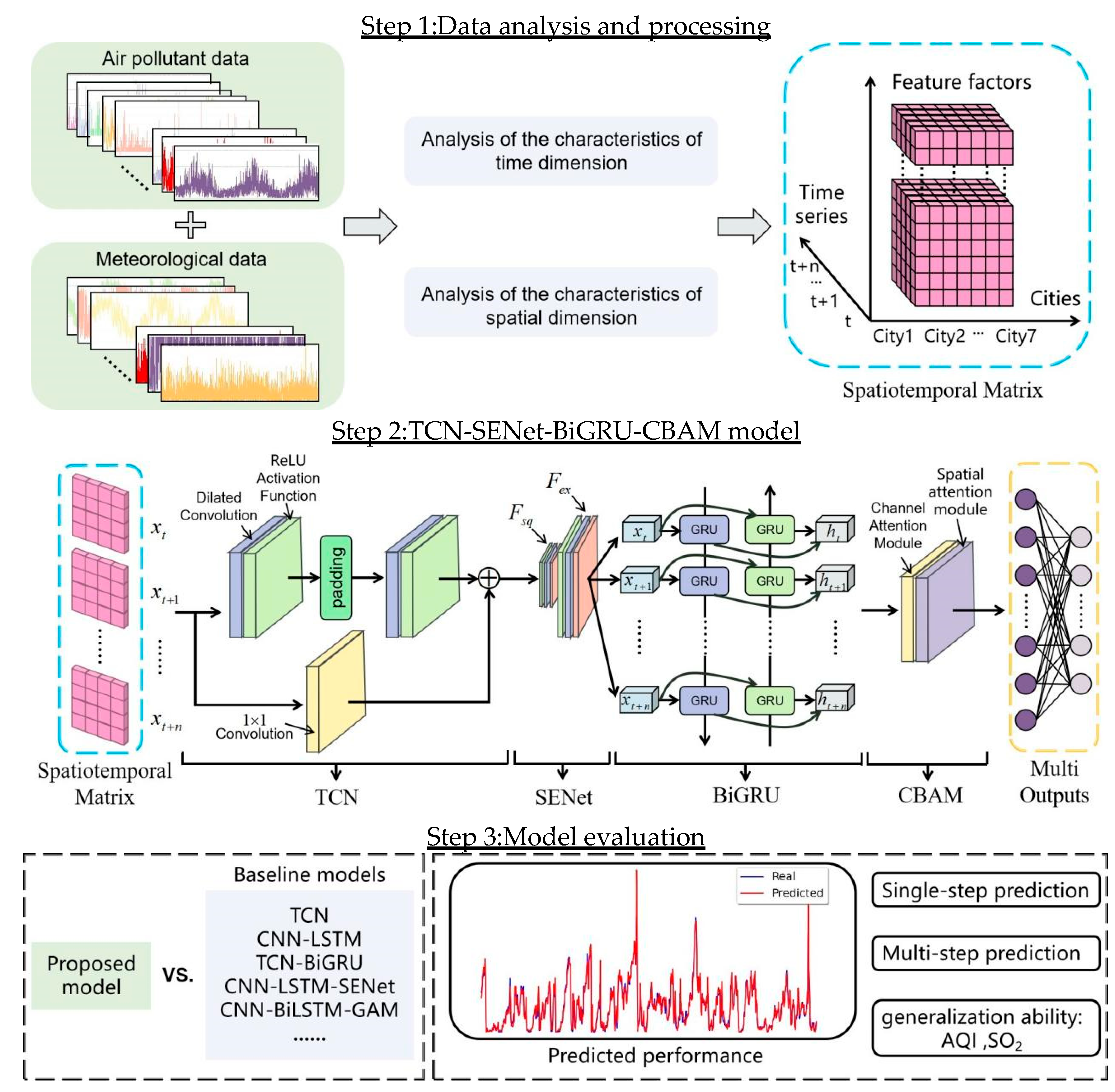
Figure 4 displays the proposed prediction system’s framework. The general framework of this study is composed of the following three major stages:

The dataset is analyzed in both temporal and spatial dimensions during the first stage, which is known as the data processing and analysis stage. The analysis’s findings in the time dimension show that the model requires air pollutants and meteorological data as inputs. The spatial dimension analysis’s findings show that air pollutants in the cities were spatially correlated, and air pollutants from other cities were taken into account while building the input features. As the model’s input, the data are transformed into a spatiotemporal matrix. This spatiotemporal matrix is a three-dimensional tensor with three dimensions: time step (the amount of time points to look back at), city, and feature (air pollutant indicators and meteorological factors).

In the second phase, the TCN-SENet-BiGRU-CBAM model is proposed, which is the core component of the system. Mapping the original inputs to the predicted outcomes is the entire training process. Inputs for TCN-SENet-BiGRU-CBAM are spatiotemporal matrices derive from historical air pollutant concentrations and meteorological data $x=\left\{x_t,x_{t+1},\dots ,x_{t+n}\right\}$. There are four layers in the model. The first layer is an improved TCN layer, where the residual connection layer in the network is moved forward into a preprocessing operation. The final output of the TCN layer is formed by adding the outputs of the two parallel transmission lines, residual connection, and dilated causal convolution element by element. TCN extracts the long-term dependency in time series data as the input of SENet. The second layer, known as the SENet layer, uses adaptive recalibration to improve the model’s representational power and gives the features new weights. The third layer, known as the BiGRU layer, creates a bi-directional feature representation for every time step by processing data from both forward and backward GRUs in the input sequence. BiGRUs make use of the sequence’s contextual information to more accurately depict intricate dependencies in time series. The CBAM layer is the fourth layer. By progressively using the channel attention and spatial attention mechanisms, CBAM dynamically modifies every component of the feature to achieve the positioning and focussing of the important regions in the sequence data. Following receipt of the CBAM output, the fully connected layer makes a final prediction. The outcome is $\widehat{y}=\left\{{\widehat{y}}_t,{\widehat{y}}_{t+1},\dots ,{\widehat{y}}_{t+r}\right\}$.

The last phase of the suggested prediction system’s framework is the model evaluation. Several metrics are calculated and the predicted values are compared with the actual values in both single-step and multi-step prediction tasks to demonstrate how much better the suggested model is than the state-of-the-art baseline models in forecasting pollutant concentrations. Lastly, we extend the model to the prediction of other air pollutant concentrations to confirm its practical application and generalization ability.

3.2. Design of the Proposed Model

3.2.1. Improved TCN Module

We improved the traditional TCN network in the following ways: the network’s residual connection layer is advanced and transformed into a preprocessing procedure, where the residual connection is handled beforehand when the model is initialized. It eliminates the need to continuously verify that the number of channels is constant during runtime. In the meantime, the issue of gradient disappearance during training can be successfully resolved and model training stability guaranteed by using residual connection. These improvements significantly reduce the computational overhead and inference time of the model, making it more practical and scalable for processing large-scale spatiotemporal air pollutant concentration data.

As illustrated in Figure 5, the enhanced TCN has two parallel transmission routes: the dilated causal convolution route and the residual connection route. In the residual connection route, the input spatiotemporal matrix will be used directly as the residual connection’s output when the number of input and output channels is consistent. If the number of input and output channels is inconsistent, a 1 × 1 convolutional layer will be used to adjust the number of input channels until it is consistent with the number of output channels. In the dilated causal convolution route, the dilated causal convolution is a fusion of dilated and causal convolution. The output of the convolution operation is only dependent on the present and past inputs, which are suitably padded to get causality. In addition, this convolution operation not only maintains causality and ensures that the model will not use future information, but also expands the receptive field through the dilation rate, so that the network can capture long-term dependencies. The dilated factor of the convolution kernel is set by dilated convolution in dilated causal convolution. The form $[{\omega }_{\theta },\theta ,{\omega }_1,\theta ,{\omega }_2]$ represents the convolution kernel’s practical application, where $\theta$ represents the distance between the convolution kernel’s elements and ${\omega }_i (i=\theta ,1,2)$ represents the kernel’s weight. The definition of the dilated causal convolution operation $F_{(s)}$ for the input of a one-dimensional time series is as follows:

$$F_{(s)}=(x\ast df) (s)= {\displaystyle \sum _{i=0}^{k-1}f(i)x_{s-d·i}}$$

(1)

where $s$ is the input sequence data, $d$ is the dilated coefficient, $k$ is the filter size, and $s-d·i$ is the historical information for reference. As shown in Figure 5, the dilated coefficient $d=(1,2,4)$. The TCN’s receptive field expands as the dilated coefficient does thus enabling to gather long-term dependent information on air pollutants and meteorology. The operational equation for the receptive field $r$ is defined as follows:

$$r=1+{\displaystyle \sum _{i=0}^{n-1}2\cdot (k-1)\cdot b^i=1+2}\cdot (k-1)\cdot {\displaystyle \frac{b^n-1}{b-1}}$$

(2)

where $n$ is the number of residual blocks, $b$ is the number of dilated bases, and $k$ is the filter size [33].

3.2.2. SENet Module

In order to improve the network’s representational capacities and better capture long-term dependencies, SENet dynamically learns the inter-channel dependencies and chooses and enhances the TCN outputs. The first step is to create a global description vector for each channel by global average pooling the height and breadth of each channel. In our case, this means pooling the time-step dimension and the city dimension. After that, two fully connected layer process the squeezed feature vectors to produce weight coefficients for every channel. Each channel’s response intensity in the original feature map is modified using these coefficients. We use the SENet module to amplify some features of the TCN output while ignoring others. Figure 6 shows the structure of SENet in the model, which includes squeezing, excitation and scaling operations [34].

Squeezing operation, which mainly compresses the spatial information of the input feature map into channel information. The Squeezing operation is represented as follows:

$$z_c=F_{sq}={\displaystyle \frac{1}{W\times H}}{\displaystyle \sum _{i=1}^H{\displaystyle \sum _{j=1}^W{x}_{i,j,c}}}$$

(3)

where $z_c$ denotes the output of the squeezing operation and $x_{i,j,c}$ denotes the eigenvalue of the $c$th channel at position $(i,j)$. The global average pooling results for each channel form a channel description vector $z={[z_1,z_2,\dots ,z_c]}^T$ of dimension $c\times 1$, which contains the global average information of the input feature maps in the spatial dimension.

Excitation operation, which is processed through two fully connected layers. The first fully connected layer reduces the feature dimension to $c/r$ and then passes the ReLU activation function. The second fully connected layer restores the feature dimension to the original $c$ dimension and generates the weight coefficients of the channels through the Sigmoid activation function to adaptively enhance or suppress the features of the different channels. The Excitation operation is denoted as follows:

$$\omega =\mathrm{Sigmoid}(W_2(\mathrm{ReLU}(W_{1}z+b_1))+b_2)$$

(4)

where $\omega$ is the channel attention weight, $W_1$ and $b_1$ are the weights and biases of the first fully connected layer, $W_2$ and $b_2$ are the weights and biases of the second fully connected layer, and $z$ is the channel description vector.

Scaling operation, multiply the channel attention weight $\omega$ obtained in the exception operation by channel $x_c$ one by one and weight it to complete the recalibration of the original features in the channel dimension. The scaling operation is represented as follows:

$${\tilde{X}}_c=F_{scale}(x_c,\omega )=x_c\cdot \omega$$

(5)

where ${\tilde{X}}_c$ is the rescaled feature map that is used as input to the next layer of the network.

3.2.3. BiGRU Module

GRU is a recursive neural network that regulates the information flow via two primary gating mechanisms: update gates and reset gates, as illustrated in Figure 7a. The GRU is represented as follows:

$$r_t=\sigma (W_r\times [x_t,h_{t-1}]+b_r)$$

(6)

$$z_t=\sigma (W_z\times [x_t,h_{t-1}]+b_z)$$

(7)

$${\tilde{h}}_t=\tanh (W_h\times [r_t\ast h_{t-1},x_t]+b_h)$$

(8)

$$h_t=(1-z_t)\ast h_{t-1}+z_t\ast {\tilde{h}}_t$$

(9)

where $r_t$ and $z_t$ denote the reset gate output and the update gate output, $W_r$, $W_z$ and $W_h$ denote the reset gate weights, the update gate weights and the hidden layer weights, $b_r$, $b_z$ and $b_h$ denote the bias vectors, $h_{t-1}$ denotes the hidden state at moment t−1, ${\tilde{h}}_t$ denotes the candidate memory content at moment t, $h_t$ denotes the hidden state at moment t, $x_t$ denotes the input feature vector, $\sigma$ denotes the Sigmoid activation function, the $\ast$ denotes the elemental multiplication, and $[]$ denotes two vectors connected to each other.

As illustrated in Figure 7b, BiGRU uses a bi-directional processing mechanism, which enables it to process the input sequence in both forward and backward directions at the same time, producing more thorough contextual information. Two independent GRU layers make up the BiGRU network: one handles the sequence’s forward information output as $h_t^f$ and the other handles its backward information output as $h_t^b$. The outputs of the two GRU layers are merged to generate a comprehensive representation of the input sequence. This bi-directional processing mechanism enhances the model’s ability to capture complex dependencies [35]. The BiGRU model is represented as follows:

$$\left\{\begin{array}{l}{h}_t^f=GRU(x_t,h_{t-1}^f) \\ h_t^b=GRU(x_t,h_{t-1}^b)\\ h_t={\omega }_t{h}_t^f+v_t{h}_t^b+b_t\end{array}\right.$$

(10)

where ${\omega }_t$ is the weight for forward propagation, $v_t$ is the weight for backward propagation, and $b_t$ is the bias value.

3.2.4. CBAM Module

The spatial attention module of CBAM operates on the spatial dimension of the feature map, assisting the model in focusing on more discriminative local regions within the output sequence of BiGRU. In contrast to SENet’s perspective, which just concentrates on channel attention, its spatial attention module assigns distinct weights to pollutant and meteorological elements of the same dimension. CBAM predicts pollutants and meteorological spatiotemporal data more effectively by taking into account both channel and spatial information at the same time. The architecture of CBAM can be expressed as follows:

$$\left\{\begin{array}{l}{F}^{\prime }=M_c(F)\times F\\ F^{″}=M_s(F^{\prime })\times F^{\prime }\end{array}\right.$$

(11)

$$M_c(F)=\sigma (\mathrm{MLP}\left(\mathrm{AvgPool}\right(F\left)\right)+\mathrm{MLP}\left(\mathrm{MaxPool}\right(F\left)\right))$$

(12)

$$M_s(F^{\prime })=\sigma \left(f^{8\times 8}([\mathrm{AvgPool}(F^{\prime });\mathrm{MaxPool}(F^{\prime }\left)\right])\right)$$

(13)

where $\times$ represents element-by-element multiplication, $M_c(F)$ represents the channel attention module, $M_s(F^{\prime })$ represents the spatial attention module, $F$ denotes the input features, MLP denotes the multilayer perceptron, $\sigma$ denotes the Sigmoid activation function, and $f^{8\times 8}$ denotes the convolution operation with a filter size of 8 × 8.

The synergistic effect of SENet and CBAM enables the model to more accurately capture the complex spatiotemporal transport and evolution patterns of pollutants and the mutual influence between neighboring regions, thereby significantly improving the reliability of predictions and the accuracy of early warnings, especially under conditions of sudden concentration changes or complex meteorological conditions.

3.3. Evaluation of the Proposed Model

3.3.1. Baseline Models

We test the suggested model with various cutting-edge deep learning models in order to evaluate its performance. To guarantee the consistency of the comparison process, the same dataset, training mode, and testing mode are employed. They are as follows:

(1)

CNN [36], Convolutional Neural Network is one of the most classical deep learning methods for predicting air pollutant concentrations. The computational complexity of the model is low.

(2)

LSTM [37], by learning long-term dependencies, Long Short-Term Memory can overcome the issue of gradient vanishing or explosion that typical RNNs face when working with lengthy sequential input. The computational complexity of the model is low.

(3)

GRU [38], Gated Recurrent Unit is a simplified version of the LSTM and performs well when dealing with sequential data. The computational complexity of the model is low.

(4)

TCN [39], Temporal Convolutional Network is a deep learning model specialized for processing time series data. The computational complexity of the model is low.

(5)

CNN-LSTM [40], The Convolutional Neural Network and Long Short-Term Memory hybrid deep learning model fully integrates and makes use of the benefits of both networks to produce improved prediction outcomes. The computational complexity of the model is moderate.

(6)

CNN-LSTM-ECA, A CNN-LSTM model incorporating the Efficient Channel Attention Module (ECA), which serves as a comparison model for the CNN-LSTM model to validate the effect of ECA. The computational complexity of the model is moderate.

(7)

CNN-LSTM-CBAM, A CNN-LSTM model incorporating the Convolutional Block Attention Module (CBAM), which serves as a comparison model for the CNN-LSTM model to validate the effect of CBAM. The computational complexity of the model is moderate.

(8)

CNN-LSTM-SENet, A CNN-LSTM model incorporating the Squeeze and Excitation Networks (SENet), which serves as a comparison model for the CNN-LSTM model to validate the effect of SENet. The computational complexity of the model is moderate.

(9)

CNN-BiLSTM-GAM, A hybrid deep learning model that incorporates a Convolutional Neural Network, a bi-directional Long Short-Term Memory and a global attention mechanism (GAM). Drawing inspiration from Rabie et al. [41], the model completes an enhanced CNN-BiLSTM model by incorporating a global attention mechanism to concentrate on the input data’s global information. The computational complexity of the model is high.

(10)

TCN-BiGRU [42], A hybrid deep learning model that combines a Temporal Convolutional Network with a bi-directional Gated Recurrent Unit is able to maintain good prediction ability in multi-step prediction and avoid random prediction. The computational complexity of the model is high.

3.3.2. Evaluation Metrics

Several evaluation metrics, such as root mean square error (RMSE), mean absolute error (MAE), R-squared (R²), and index of agreement (IA), are utilized to evaluate the validity and accuracy of the suggested prediction method. The following formula is used to determine these experimental metrics:

$$\mathrm{RMES}=\sqrt{{\displaystyle \frac{{\displaystyle {\sum }_{\mathrm{i}=1}^{\mathrm{T}}{(y_i-{\widehat{y}}_i)}^2}}{\mathrm{T}}}}$$

(14)

$$\mathrm{MAE}={\displaystyle \frac{1}{\mathrm{T}}}{\displaystyle \sum _{\mathrm{i}=1}^{\mathrm{T}}\left|y_i-{\widehat{y}}_i\right|}$$

(15)

$${\mathrm{R}}^2=1-{\displaystyle \frac{{\displaystyle \sum _{\mathrm{i}=1}^{\mathrm{T}}{(y_i-{\widehat{y}}_i)}^2}}{{\displaystyle \sum _{\mathrm{i}=1}^{\mathrm{T}}{(y_i-\overline{y})}^2}}}$$

(16)

$$\mathrm{IA}=1-{\displaystyle \frac{{\displaystyle \sum _{\mathrm{i}=1}^{\mathrm{T}}{(y_i-{\widehat{y}}_i)}^2}}{{\displaystyle \sum _{\mathrm{i}=1}^{\mathrm{T}}{(\left|y_i-\overline{y}\right|+\left|{\widehat{y}}_i-\overline{y}\right|)}^2}}}$$

(17)

where $y_i$ is the observed value, ${\widehat{y}}_i$ is the predicted value, $\mathrm{T}$ is the test set size, and $\overline{y}$ is the average observed value.

4. Experiment and Results

4.1. Hyperparameter Setting

A validation set of 10% of the dataset is chosen, and multiple iterations of experiments are carried out to determine the optimal collection of hyperparameters. The precise procedure is as follows: for each experiment, we set the batch size at 256 and the number of training cycles (epoch) at 50. We then evaluate the model’s performance by calculating the RMSE and MAE, and if they drop, we modify and store the current model parameters. The collection of hyperparameters that produced the best prediction on the validation set was chosen for the final model following a number of tests and parameter adjustments. The precise parameter configurations utilized for the final model following experimentation are listed in

Table 3. Model hyperparameter.

Layer Name		Hyperparameter	Values
TCN		[filter, channel] $\times$ number of layers	[3 $\times$ 3128] $\times$ 1
SENet		[layour nodes] $\times$ number of layers	[128] $\times$ 2
BiGRU		[layour nodes] $\times$ number of layers	[16] $\times$ 1
CBAM	Channel attention	-	-
	Spatial attention	[filter, channel] $\times$ number of layers	[8 $\times$ 8.1] $\times$ 1 [1 $\times$ 1.8] × 1
-		Batch size	256
-		Epochs	50
-		Step	10
-		Learning rate	0.0005
-		Training method	Adam

.

4.2. Single-Step Prediction

The device used in this study is a Windows 10 system with the following basic configuration: CPU: i7-9750 @ 2.60 GHz, GPU: NVIDIA GeForce GTX1650 4GB, and RAM: 8G. The Python version used is Python 3.9.12. During data processing, model construction, training, and testing, open-source libraries and frameworks such as PyTorch 2.2.2, Pandas, NumPy, scikit-learn, and matplotlib were utilized.

The single-step prediction experiment’s window size is three hours, with twenty-two features, and the prediction step is one. This task’s objective is to predict Beijing’s PM₂.₅ concentration for the upcoming hour using the last 3-hour feature data.

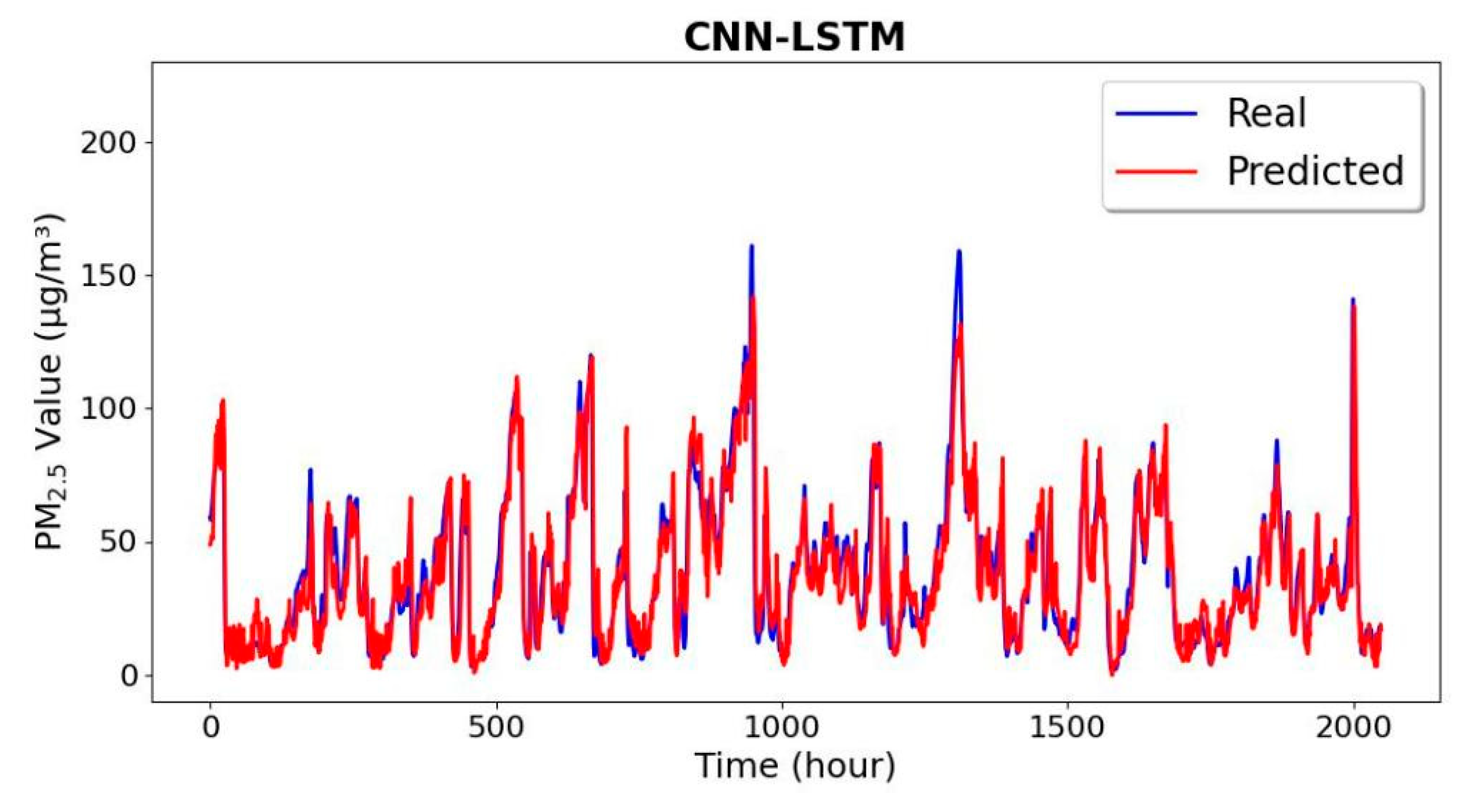
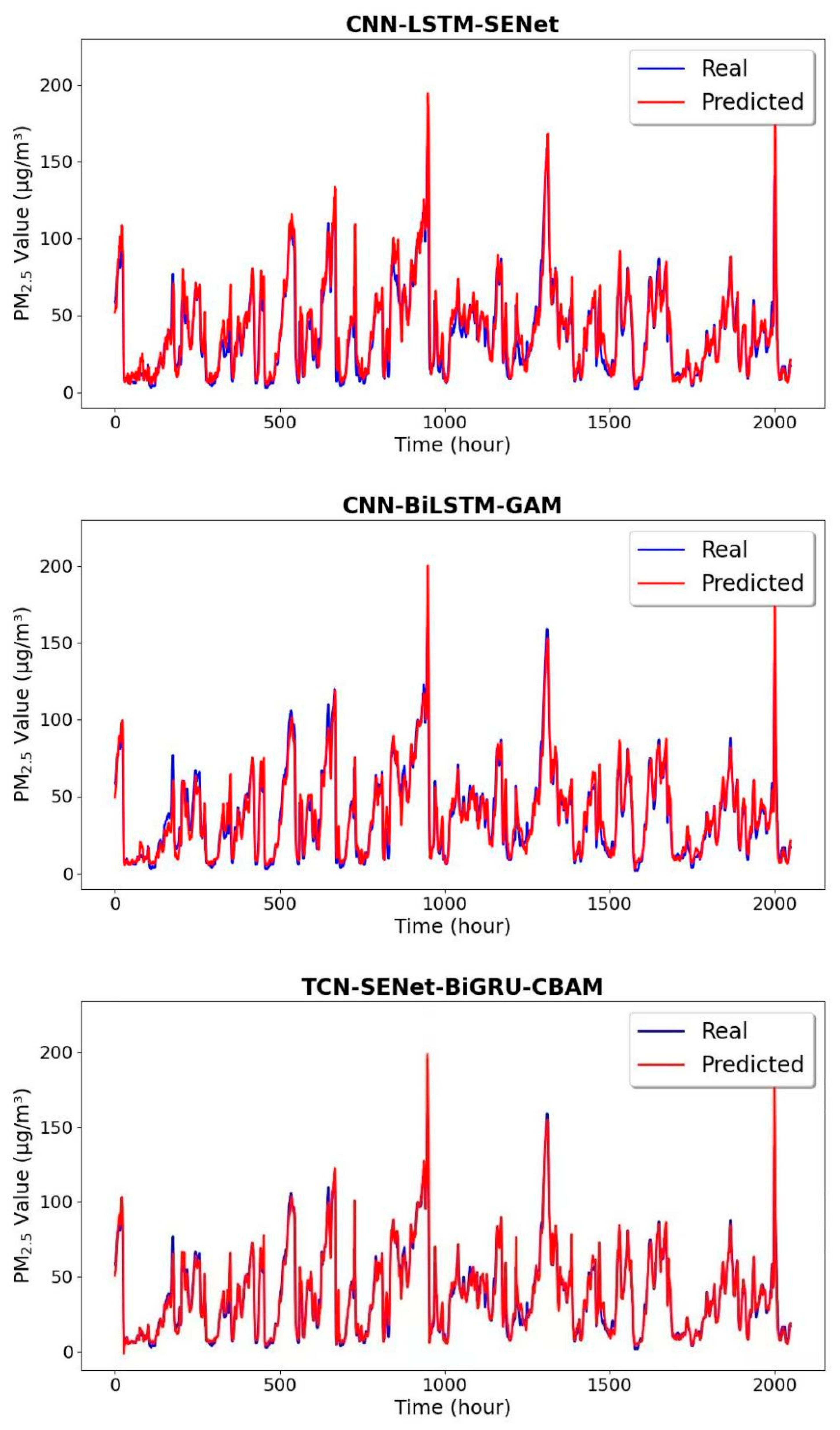
The fitting diagram of the actual and predicted values of the suggested model and the other three baseline models was created using the first 2050 h in a row that were taken out of the test set, as seen in Figure 8. The predicted value curve is red, but the actual value curve is blue. The TCN-SENet-BiGRU-CBAM model’s predicted value curve, as shown in the figure, has the best fit to the actual value curve and outperforms the other three baseline models at the mutation point, peak valley point, and time period with more intense fluctuations. The evaluation of the proposed model’s prediction performance in comparison to ten other models with the same epoch, batch size, and learning rate is summarized in

Table 4. Comparison of single-step prediction performance of different models.

Model	RMSE	MAE	R2	IA
CNN	11.669	7.428	0.838	0.931
LSTM	10.855	7.823	0.868	0.941
GRU	10.347	7.367	0.804	0.946
TCN	9.037	6.044	0.854	0.961
CNN-LSTM	9.099	6.454	0.866	0.958
CNN-LSTM-ECA	9.632	6.387	0.853	0.955
CNN-LSTM-CBAM	8.524	5.478	0.875	0.965
CNN-LSTM-SENet	8.290	5.339	0.885	0.968
CNN-BiLSTM-GAM	6.427	4.355	0.924	0.980
TCN-BiGRU	6.370	4.204	0.924	0.980
TCN-SENet-BiGRU-CBAM	5.309	3.507	0.949	0.987

. Evaluation metrics include RMSE, MAE, R², and IA. The closer RMSE and MAE values are to 0, the lower the model’s prediction error and the better the model’s performance; the closer R² and IA values are to 1, the better the model fits the actual data and the more accurately it explains it. It is evident from the comparison that our TCN-SENet-BiGRU-CBAM model performs the best and has the best prediction effect.

Furthermore, the first 2050 h in a row were selected from the test set, and Figure 9 displays the scatter plots of the actual vs. predicted values of the proposed model in comparison to the other three baseline models. The red dashed line represents the function y = x, the vertical axis represents the actual PM₂.₅ levels, and the horizontal axis represents the predicted PM₂.₅ values. The figure illustrates that, in comparison to the other three baseline models, the TCN-SENet-BiGRU-CBAM model exhibits the least degree of dispersion and the least dispersion of outliers. CNN-LSTM, CNN-LSTM-SENet, CNN-BiLSTM-GAM, and TCN-SENet-BiGRU-CBAM have R² values of 0.866, 0.885, 0.924, and 0.949, respectively. This suggests that the actual and predicted values of the TCN-SENet-BiGRU-CBAM model are highly correlated. Thus, in the single-step prediction test of air pollutants, it is confirmed that our proposed model has superior prediction performance and prediction accuracy.

4.3. Multi-Step Prediction

When predicting PM₂.₅ concentrations in a practical application scenario, it is typically required to forecast data for a longer time frame in the future using past data. Consequently, it is necessary to look into multi-step PM₂.₅ concentration prediction. As seen in Figure 10, multi-step prediction is the process of predicting the values of several consecutive future time points utilizing a period of historical data [43].

4.3.1. The Performance of the Proposed Model in Different Situations

The performance of the proposed TCN-SENet-BiGRU-CBAM model for predicting concentrations of PM₂.₅ over the next one to twelve hours is investigated. The model was given various window sizes and prediction steps to compute the model performance evaluation metrics at this point, which are RMSE, MAE, R², and IA, as indicated in

Table 5. Multi step prediction with different window sizes and prediction step sizes.

Prediction Step Sizes (Hour)	Window Sizes (Hour)	RMSE	MAE	R2	IA
1–2 h	4 h	6.917	4.472	0.910	0.977
1–2 h	6 h	6.455	4.017	0.922	0.979
1–3 h	6 h	7.751	4.810	0.887	0.970
1–6 h	10 h	11.151	6.928	0.767	0.931
1–8 h	12 h	12.537	7.835	0.705	0.915
1–12 h	16 h	14.043	9.200	0.630	0.885

.

The relationship is seen in Table 5 when the quantity of historical data input is increased concurrently with the prediction step. Table 5 shows that, while the prediction step remains constant, the model’s accuracy in predicting PM₂.₅ concentration rises as the input historical data lengthens from 4 to 6 h. However, while increasing the input of historical data to improve the accuracy of the model, the rise in prediction cost should also be considered, as the RMSE and MAE only increased by 0.462 and 0.455, respectively. As the prediction step size grows, the TCN-SENet-BiGRU-CBAM model’s prediction accuracy declines, with the RMSE rising from 6.917 to 14.043 and the MAE rising from 4.472 to 9.200. The numerous tests that follow demonstrate how well the proposed model fits multi-step prediction problems.

4.3.2. Ablation Experiments on the Proposed Model

Ablation experiments on TCN-SENet-BiGRU-CBAM were carried out in this section to investigate how the channel attention mechanism SENet and the hybrid attention mechanism CBAM affect the model’s ability to extract spatiotemporal features.

Table 6. Ablation experiment for multi-step prediction of PM₂.₅.

Model	1–6 h Prediction		1–12 h Prediction
	RMSE	MAE	RMSE	MAE
TCN	15.817	11.005	18.054	13.046
BiGRU	13.469	9.439	16.555	11.680
BiGRU-CBAM	12.629	8.141	15.784	10.760
TCN-SENet	12.325	7.898	15.167	9.958
TCN-BiGRU	12.190	8.058	16.483	11.492
TCN-SENet-BiGRU	12.115	7.665	15.333	10.289
TCN-BiGRU-CBAM	11.551	7.327	14.534	9.495
TCN-SENet-BiGRU-CBAM	11.151	6.928	14.043	9.200

presents the experimental outcomes.

The first step is to examine how the model is affected by the channel attention mechanism SENet. In comparison to the TCN-SENet-BiGRU-CBAM model, the prediction accuracies of BiGRU-CBAM, TCN-BiGRU, and TCN-BiGRU-CBAM are all reduced when the SENet module is eliminated. Furthermore, the prediction accuracies on the 1–6 h and 1–12 h prediction tasks are improved when the TCN module and SENet are combined. It demonstrates that SENet can, in fact, increase the model’s prediction accuracy because, as a channel attention mechanism, it uses the special squeeze excitation mechanism to learn the features output from the TCN secondarily. This allows the network to perceive features that are far from the current position and significantly enhances its capacity to capture long-term dependent features. The effect is more pronounced for longer prediction tasks. For instance, TCN-SENet outperforms TCN-BiGRU in the 1–12 h prediction task.

The impact of the CBAM on the model is then examined. In comparison to the TCN-SENet-BiGRU-CBAM model, the prediction accuracies of TCN-SENet, TCN-BiGRU, and TCN-SENet-BiGRU are all reduced when the CBAM module is eliminated. Furthermore, the prediction accuracy on the 1–6 h and 1–12 h prediction tasks increases when the BiGRU module and CBAM are combined. It indicates that CBAM can also improve the prediction accuracy of the model. The spatial attention mechanism of CBAM acts on the spatial dimension of the feature map and can adaptively focus on the more critical parts of the BiGRU output sequence.

4.3.3. Comparative Experiments with Other Models

We used MAE as a metric to evaluate the accuracy of the various models for each time period (1–3, 4–6, 7–9, and 10–12 h) in a forecasting cycle, with a predicting step of 12 h into the future and an input length of 16 h of historical data. The proposed model outperforms the other baseline models in terms of prediction accuracy throughout all time periods, as indicated in

Table 7. MAE for each time period within a prediction cycle.

Model	1–3 h	4–6 h	7–9 h	10–12 h
CNN-LSTM	10.628	12.204	13.091	13.942
CNN-LSTM-SENet	9.617	11.342	12.519	13.440
CNN-BiLSTM-GAM	6.508	9.337	11.431	12.905
TCN-BiGRU	8.647	10.779	13.054	13.671
TCN-SENet-BiGRU-CBAM	5.326	8.502	11.001	12.409

.

We used the situations of prediction step sizes of 6 h and 12 h as examples to visually illustrate the performance of TCN-SENet-BiGRU-CBAM in multi-step prediction tasks. The fit of the true values to the predicted values was plotted, as seen in Figure 11, using four consecutive and random prediction intervals each time.

4.4. Experiment on the Generalization Ability of the Proposed Model

To show the models’ capacity for generalization, the proposed TCN-SENet-BiGRU-CBAM is used to predict the Air Quality Index (AQI) and SO₂, and its results are compared with other deep learning models. We split the next twelve hours into six tasks: one single-step prediction and five multi-step predictions. The evaluation metrics of each model in the AQI prediction task and the SO₂ prediction task are displayed in

Table 8. Single-step prediction and multi-step prediction of AQI.

Model		Prediction Step Sizes (Hour)
		1–1 h	1–2 h	1–3 h	1–6 h	1–8 h	1–12 h
CNN-LSTM	RMSE	22.482	22.517	26.930	29.305	30.527	32.255
	MAE	12.489	11.315	14.835	16.324	17.213	19.137
CNN-LSTM-SENet	RMSE	17.243	21.327	24.732	28.721	30.291	31.725
	MAE	8.715	10.619	12.526	15.549	16.885	18.019
CNN-BiLSTM-GAM	RMSE	13.839	16.945	20.314	26.005	27.474	30.720
	MAE	6.802	8.065	10.190	12.213	14.054	17.005
TCN-BiGRU	RMSE	13.321	17.697	19.161	24.237	27.233	29.316
	MAE	7.820	9.084	9.179	11.665	14.231	15.868
TCN-SENet-BiGRU-CBAM	RMSE	10.414	14.146	17.204	24.029	26.871	29.080
	MAE	5.079	6.448	7.569	11.315	12.794	14.294

and

Table 9. Single-step prediction and multi-step prediction of SO₂.

Model		Prediction Step Sizes (Hour)
		1–1 h	1–2 h	1–3 h	1–6 h	1–8 h	1–12 h
CNN-LSTM	RMSE	0.608	0.826	1.046	1.048	0.971	1.057
	MAE	0.445	0.549	0.576	0.600	0.625	0.625
CNN-LSTM-SENet	RMSE	0.583	0.664	0.735	0.886	0.905	0.957
	MAE	0.396	0.432	0.473	0.585	0.583	0.612
CNN-BiLSTM-GAM	RMSE	0.510	0.571	0.635	0.740	0.768	0.833
	MAE	0.333	0.374	0.408	0.475	0.475	0.508
TCN-BiGRU	RMSE	0.492	0.614	0.659	0.811	0.849	1.000
	MAE	0.317	0.386	0.445	0.539	0.555	0.603
TCN-SENet-BiGRU-CBAM	RMSE	0.481	0.544	0.602	0.711	0.754	0.806
	MAE	0.312	0.345	0.376	0.454	0.470	0.498

, respectively.

Table 8 and Table 9 demonstrate that TCN-SENet-BiGRU-CBAM has the best prediction ability and the highest prediction accuracy for both AQI and SO₂ when compared to other deep learning models. It demonstrates the effectiveness of the proposed model as a forecast tool for air pollution concentrations with strong generalization capabilities.

5. Discussion

5.1. Analyze the Results of Single-Step Prediction

When compared to individual deep learning models, Table 4 demonstrates that hybrid deep learning models produce higher prediction outcomes. The benefits of several modules can be combined by CNN-LSTM, CNN-LSTM-ECA, CNN-LSTM-CBAM, CNN-LSTM-SENet, CNN-BiLSTM-GAM, TCN-BiGRU, and TCN-SENet-BiGRU-CBAM to extract more detailed aspects of pollutants and meteorological data. Each model’s performance is evaluated using RMSE ranging from 5.309 to 11.669, MAE ranging from 3.507 to 7.823, R² ranging from 0.804 to 0.949, and IA ranging from 0.931 to 0.987.

Applying a reasonable attention mechanism is beneficial for enhancing the model’s performance and feature extraction capabilities, as demonstrated by the comparison of CNN-LSTM with CNN-LSTM-ECA, CNN-LSTM-CBAM, and CNN-LSTM-SENet that integrate the attention mechanism. When CNN-LSTM-ECA, CNN-LSTM-CBAM, and CNN-LSTM-SENet are compared, it is evident that CBAM and SENet outperform ECA in terms of enhancing prediction model performance. This demonstrates that CBAM and SENet are better suited for the task of predicting the concentration of air pollutants. Combining CBAM with SENet can assist the model better focus on spatiotemporal features of the data, respectively, increasing the prediction accuracy.

It is evident that TCN-BiGRU has a substantially poorer accuracy when compared to TCN-SENet-BiGRU-CBAM. Through a sensible design, TCN-SENet-BiGRU-CBAM efficiently combines the strengths of SENet and CBAM in feature extraction while also improving the efficiency of information flow between the TCN and BiGRU layers. TCN-SENet-BiGRU-CBAM is shown to have a better understanding and expression of air pollutants and meteorological sequence data over an extended period of time after comparing other hybrid deep learning models in Table 4.

To further confirm TCN-SENet-BiGRU-CBAM’s prediction ability for periods with high frequency of PM₂.₅ concentration changes, we chose the first 2050 consecutive time points in the test set to visualize the fitting of the true values to the predicted values, as shown in Figure 8 and 9. It is evident that the comparison model’s prediction results at periods with intense concentration fluctuations, as well as at peaks and valleys and sudden change points, are not consistent with the trend of the true values, indicating that it is challenging to make a better prediction when faced with complex situations. On the other hand, our proposed TCN-SENet-BiGRU-CBAM’s predicted results are essentially in line with the actual values, which allows it to more effectively handle difficult situation prediction.

Comparing the performance of each model in Figure 8 and Figure 9, (1) it is evident that TCN-SENet-BiGRU-CBAM is better able to adjust to the complex and variable real situation in the pollutant concentration prediction task than the comparison model; (2) in Figure 9, the comparison model’s scatter point dispersion is greater than that of the proposed model for PM₂.₅ concentrations exceeding 100, indicating that TCN-SENet-BiGRU-CBAM has a higher prediction accuracy for high PM₂.₅ concentrations; (3) combining Figure 8 and Figure 9, it is frequently difficult to fit the true values at the mutation point with the predicted values, which shows up in the scatter plot as discrete values. This is because there are few samples of mutation points in the dataset and the many factors that generate mutation points are highly uncertain, so it is difficult for the prediction model to learn the pattern of mutation behavior from a limited number of samples. This phenomenon poses a challenge for pollutant concentration prediction models in predicting some mutation behaviors.

5.2. Analyze the Results of Multi-Step Prediction

In real-world applications, such monitoring and managing urban air quality, a 12-hour prediction step is adequate to give prompt alerts that enable the department to implement interim countermeasures. As a result, we decided to set a 12-hour maximum prediction step. Table 5 and Table 7 demonstrate that TCN-SENet-BiGRU-CBAM outperforms the comparison models in a variety of multi-step prediction tasks and has greater prediction accuracies. TCN-SENet-BiGRU-CBAM achieves satisfactory results with RMSE and MAE values of 14.043 and 9.200, respectively, even facing a 12-hour prediction step.

As shown in Table 6, we investigated the effect of each module of TCN-SENet-BiGRU-CBAM on the model performance. The results of the ablation experiments show that the attention mechanisms SENet and CBAM can effectively improve the prediction performance of the model. TCN-SENet-BiGRU-CBAM’s performance on four random and continuous prediction intervals with 6-hour and 12-hour prediction steps is displayed in Figure 11. It is evident that overall, the pattern of change between the blue true value curve and the red predicted value curve is the same. The ability of TCN-SENet-BiGRU-CBAM to complete the long-term air pollutant concentration prediction tasks has been demonstrated by numerous studies.

5.3. Analyze the Generalization Ability of the Proposed Model

Since TCN-SENet-BiGRU-CBAM performed well in predicting Beijing’s PM₂.₅ concentration, we expanded the model to forecast other air pollutant concentrations, including AQI and SO₂. The final experimental findings show that the model is more robust and has a higher ability to generalize. Thus, this paper’s research offers a novel approach to building models for deep learning air pollutant concentration prediction, enhances prediction performance and accuracy, and is anticipated to serve as a foundation for air pollution warning and prevention.

6. Conclusions

A novel hybrid deep learning model is developed in this study to achieve the prediction of concentrations of air pollutants. First, the selection of model input features is guided by the use of Pearson correlation analysis for the study area’s air pollutants and meteorological data. Then, by making full use of the attention mechanisms SENet and CBAM’s extraction capabilities on spatiotemporal features, the TCN-SENet-BiGRU-CBAM prediction model was built. The model’s TCN module is enhanced in comparison to the conventional TCN by converting the network’s residual connection into preprocessing processes, which boosts the model’s performance and operational efficiency. The proposed model performs better than other advanced baseline models in terms of prediction accuracy and performance, according to the experimental findings of single-step and multi-step prediction. By adding SENet and CBAM, the model can better understand and localize to deeper features than single-structured models like CNN and TCN. It can also make better predictions during periods of intense concentration fluctuations, as well as at peaks and troughs and mutation points. In the prediction task of PM₂.₅ in Beijing, the root mean square error (RMSE) and mean absolute error (MAE) of the proposed model are in the range of 5.309~14.043 and 3.507~9.200, respectively. Lastly, the model’s robustness and great generalization ability are demonstrated by its excellent performance in predicting the concentrations of other air pollutants. The comprehensive improvement in accuracy and performance of the TCN-SENet-BiGRU-CBAM model provides a strong technical foundation for building a more reliable regional air pollution prediction and warning system. It is expected to become the basis for air pollution warning and prevention. Here is a summary of this paper’s primary contributions:

(1)

A scientific dataset creation method based on spatio-temporal correlation analysis is demonstrated, taking into account air pollutants with a high degree of connection in other cities outside the prediction area;

(2)

Improvement of the traditional TCN network: the network’s residual connection layer is moved ahead and transformed into a preprocessing function. It enhances the model’s performance and operational efficiency while lowering runtime overhead;

(3)

Following the TCN layer, the channel attention mechanism SENet is introduced, which enhances prediction performance and accuracy by efficiently extracting the long-term dependent features of pollutants and meteorological data;

(4)

Introducing the hybrid attention mechanism CBAM. The feature map spatial dimension attention mechanism of CBAM helps the model focus on key local patterns in the output sequence of BiGRU.

Although the prediction methods proposed in this research have been proven to be superior and applicable, there is yet room for improvement. The next step will involve adding data from multiple monitoring stations in each region as independent features to introduce richer spatial information.

References

1. Chen, J.; Yuan, C.; Dong, S.; Feng, J.; Wang, H. A novel spatiotemporal multigraph convolutional network for air pollution prediction. Appl. Intell. 2023, 53, 18319–18332. [Google Scholar] [CrossRef]
2. Wan, K.; Shackley, S.; Doherty, R.; Shi, Z.; Zhang, P.; Golding, N. Science-policy interplay on air pollution governance in China. Environ. Sci. Policy 2020, 107, 150–157. [Google Scholar] [CrossRef]
3. Morawska, L.; Zhu, T.; Liu, N.; Torkmahalleh, M.A.; Andrade, M.F.; Barratt, B.; Broomandi, P.; Buonanno, G.; Ceron, L.C.B.; Chen, J.; et al. The state of science on severe air pollution episodes: Quantitative and qualitative analysis. Environ. Int. 2021, 156, 106732. [Google Scholar] [CrossRef]
4. Huang, G.; Ge, C.; Xiong, T.; Song, S.; Yang, L.; Liu, B.; Yin, W.; Wu, C. Large scale air pollution prediction with deep convolutional networks. Sci. China Inf. Sci. 2021, 64, 192107. [Google Scholar] [CrossRef]
5. Gu, Y.; Li, B.; Meng, Q. Hybrid interpretable predictive machine learning model for air pollution prediction. Neurocomputing 2022, 468, 123–136. [Google Scholar] [CrossRef]
6. Bekkar, A.; Hssina, B.; Douzi, S.; Douzi, K. Air-pollution prediction in smart city, deep learning approach. J. Big Data 2021, 8, 161. [Google Scholar] [CrossRef]
7. Zhang, Z.; Zhang, S.; Chen, C.; Yuan, J. A systematic survey of air quality prediction based on deep learning. Alexandria Eng. J. 2024, 93, 128–141. [Google Scholar] [CrossRef]
8. Gong, S.; Zhang, L.; Liu, C.; Lu, S.; Pan, W.; Zhang, Y. Multi-scale analysis of the impacts of meteorology and emissions on PM2.5 and O3 trends at various regions in China from 2013 to 2020 2. Key weather elements and emissions. Sci. Total Environ. 2022, 824, 153847. [Google Scholar] [CrossRef]
9. Wang, K.; Ling, C.; Chen, Y.; Zhang, Z. Spatio-temporal joint modelling on moderate and extreme air pollution in Spain. Environ. Ecol. Stat. 2023, 30, 601–624. [Google Scholar] [CrossRef]
10. Lalik, K.; Kozak, J.; Podlasek, S.; Kozek, M. Self-powered wireless sensor matrix for air pollution detection with a neural predictor. Energies 2022, 15, 1962. [Google Scholar] [CrossRef]
11. Hilal, A.M.; Al-Wesabi, F.N.; Alajmi, M.; Eltahir, M.M.; Medani, M.; Duhayyim, M.A. Machine learning-based Decision Tree J48 with grey wolf optimizer for environmental pollution control. Environ. Technol. 2023, 44, 1973–1984. [Google Scholar] [CrossRef]
12. Niu, C.; Niu, Z.; Qu, Z.; Wei, L.; Li, Y. Research and application of the mode decomposition-recombination technique based on sample-fuzzy entropy and K-means for air pollution forecasting. Front. Environ. Sci. 2022, 10, 941405. [Google Scholar] [CrossRef]
13. Liu, W.; Guo, G.; Chen, F.; Chen, Y. Meteorological pattern analysis assisted daily PM2.5 grades prediction using SVM optimized by PSO algorithm. Atmos. Pollut. Res. 2019, 10, 1482–1491. [Google Scholar] [CrossRef]
14. Yang, J.; Tian, Y.; Wu, C.H. Air Quality Prediction and Ranking Assessment Based on Bootstrap-XGBoost Algorithm and Ordinal Classification Models. Atmosphere 2024, 15, 925. [Google Scholar] [CrossRef]
15. Zheng, H.; Cheng, Y.; Li, H. Investigation of model ensemble for fine-grained air quality prediction. China Commun. 2020, 17, 207–223. [Google Scholar] [CrossRef]
16. Pan, K.; Lu, J.; Li, J.; Xu, Z. A Hybrid Autoformer Network for Air Pollution Forecasting Based on External Factor Optimization. Atmosphere 2023, 14, 869. [Google Scholar] [CrossRef]
17. Yang, C.H.; Chen, P.H.; Wu, C.H.; Yang, C.S.; Chuang, L.Y. Deep learning-based air pollution analysis on carbon monoxide in Taiwan. Ecol. Inform. 2024, 80, 102477. [Google Scholar] [CrossRef]
18. Ragab, M.G.; Abdulkadir, S.J.; Aziz, N.; Al-Tashi, Q.; Alyousifi, Y.; Alhussian, H. A Novel One-Dimensional CNN with Exponential Adaptive Gradients for Air Pollution Index Prediction. Sustainability 2020, 12, 10090. [Google Scholar] [CrossRef]
19. Chang, Y.S.; Chiao, H.T.; Abimannan, S.; Huang, Y.P.; Tsai, Y.T.; Lin, K.M. An LSTM-based aggregated model for air pollution forecasting. Atmos. Pollut. Res. 2020, 11, 1451–1463. [Google Scholar] [CrossRef]
20. Saif-ul-Allah, M.W.; Qyyum, M.A.; Ul-Haq, N.; Salman, C.A.; Ahmed, F. Gated recurrent unit coupled with projection to model plane imputation for the PM2.5 prediction for Guangzhou City, China. Front. Environ. Sci. 2022, 9, 816616. [Google Scholar] [CrossRef]
21. Samal, K.K.R.; Panda, A.K.; Babu, K.S.; Das, S.K. Multi-output TCN autoencoder for long-term pollution forecasting for multiple sites. Urban Clim. 2021, 39, 100943. [Google Scholar] [CrossRef]
22. Zhang, B.; Liu, Y.; Yong, R.; Zou, G.; Yang, R.; Pan, J.; Li, M. A spatial correlation prediction model of urban PM2.5 concentration based on deconvolution and LSTM. Neurocomputing 2023, 544, 126280. [Google Scholar] [CrossRef]
23. Zhu, X.; Zou, F.; Li, S. Enhancing Air Quality Prediction with an Adaptive PSO-Optimized CNN-Bi-LSTM Model. Appl. Sci. 2024, 14, 5787. [Google Scholar] [CrossRef]
24. Faraji, M.; Nadi, S.; Ghaffarpasand, O.; Homayoni, S.; Downey, K. An integrated 3D CNN-GRU deep learning method for short-term prediction of PM2.5 concentration in urban environment. Sci. Total Environ. 2022, 834, 155324. [Google Scholar] [CrossRef]
25. Zhang, B.; Zou, G.; Qin, D.; Ni, Q.; Mao, H.; Li, M. RCL-Learning: ResNet and convolutional long short-term memory-based spatiotemporal air pollutant concentration prediction model. Expert Syst. Appl. 2022, 207, 118017. [Google Scholar] [CrossRef]
26. Chen, C.; Qiu, A.; Chen, H.; Chen, Y.; Liu, X.; Li, D. Prediction of pollutant concentration based on spatial–temporal attention, ResNet and ConvLSTM. Sensors 2023, 23, 8863. [Google Scholar] [CrossRef]
27. Li, D.; Liu, J.; Zhao, Y. Prediction of multi-site PM2.5 concentrations in Beijing using CNN-Bi LSTM with CBAM. Atmosphere 2022, 13, 1719. [Google Scholar] [CrossRef]
28. Li, D.; Wang, J.; Tian, D.; Chen, C.; Xiao, X.; Wang, L. Residual neural network with spatiotemporal attention integrated with temporal self-attention based on long short-term memory network for air pollutant concentration prediction. Atmos. Environ. 2024, 329, 120531. [Google Scholar] [CrossRef]
29. Wu, J.; Zhu, J.; Li, W.; Xu, D.; Liu, J. Estimation of the PM2.5 health effects in China during 2000–2011. Environ. Sci. Pollut. Res. 2017, 24, 10695–10707. [Google Scholar] [CrossRef] [PubMed]
30. Yan, R.; Liao, J.; Yang, J.; Sun, W.; Nong, M.; Li, F. Multi-hour and multi-site air quality index forecasting in Beijing using CNN, LSTM, CNN-LSTM, and spatiotemporal clustering. Expert Syst. Appl. 2021, 169, 114513. [Google Scholar] [CrossRef]
31. Zhang, B.; Zou, G.; Qin, D.; Lu, Y.; Jin, Y.; Wang, H. A novel Encoder-Decoder model based on read-first LSTM for air pollutant prediction. Sci. Total Environ. 2021, 765, 144507. [Google Scholar] [CrossRef]
32. Hu, J.; Wang, Y.; Ying, Q.; Zhang, H. Spatial and temporal variability of PM2.5 and PM10 over the North China Plain and the Yangtze River Delta, China. Atmos. Environ. 2014, 95, 598–609. [Google Scholar] [CrossRef]
33. Ren, Y.; Wang, S.; Xia, B. Deep learning coupled model based on TCN-LSTM for particulate matter concentration prediction. Atmos. Pollut. Res. 2023, 14, 101703. [Google Scholar] [CrossRef]
34. Zhang, G.; Choi, D.; Jung, J. Development of continuous cuffless blood pressure prediction platform using enhanced 1-D SENet-LSTM. Expert Syst. Appl. 2024, 242, 122812. [Google Scholar] [CrossRef]
35. Yang, F.; Huang, G. An optimized decomposition integration model for deterministic and probabilistic air pollutant concentration prediction considering influencing factors. APR 2024, 15, 102144. [Google Scholar] [CrossRef]
36. Sayeed, A.; Choi, Y.; Eslami, E.; Lops, Y.; Roy, A.; Jung, J. Using a deep convolutional neural network to predict 2017 ozone concentrations, 24 hours in advance. Neural Netw. 2020, 121, 396–408. [Google Scholar] [CrossRef] [PubMed]
37. Li, X.; Peng, L.; Yao, X.; Cui, S.; Hu, Y.; You, C. Long short-term memory neural network for air pollutant concentration predictions: Method development and evaluation. Environ. Pollut. 2017, 231, 997–1004. [Google Scholar] [CrossRef]
38. Ayturan, Y.A.; Ayturan, Z.C.; Altun, H.O.; Kongoli, C.; Tuncez, F.D.; Dursun, Ş. Short-term prediction of PM2.5 pollution with deep learning methods. Glob. Nest J. 2020, 1, 22. [Google Scholar]
39. Huang, J.; Liu, S.; Hassan, S.G.; Xu, L. Pollution index of waterfowl farm assessment and prediction based on temporal convoluted network. PLoS ONE 2021, 16, e0254179. [Google Scholar] [CrossRef]
40. Li, T.; Hua, M.; Wu, X.U. A hybrid CNN-LSTM model for forecasting particulate matter (PM2.5). IEEE Access 2020, 8, 26933–26940. [Google Scholar] [CrossRef]
41. Rabie, R.; Asghari, M.; Nosrati, H.; Niri, M.E.; Karimi, S. Spatially resolved air quality index prediction in megacities with a CNN-Bi-LSTM hybrid framework. Sustain. Cities Soc. 2024, 109, 105537. [Google Scholar] [CrossRef]
42. Shi, T.; Li, P.; Yang, W.; Qi, A.; Qiao, J. Application of TCN-biGRU neural network in PM2.5 concentration prediction. Environ. Sci. Pollut. Res. 2023, 30, 119506–119517. [Google Scholar] [CrossRef]
43. Zhang, K.; Yang, X.; Cao, H.; Thé, J.; Tan, Z.; Yu, H. Multi-step forecast of PM2.5 and PM10 concentrations using convolutional neural network integrated with spatial-temporal attention and residual learning. Environ. Int. 2023, 171, 107691. [Google Scholar] [CrossRef]
Figure 1. Study area.
Applsci 15 09274 g001
Figure 2. Time series chart of air pollutants and meteorology, (at) represents PM2.5, PM2.5_24 h, PM10, PM10_24 h, SO2, SO2_24 h, NO2, NO2_24 h, O3, O3_8h, CO, CO_24 h, Temperature, Surface pressure, Relative humidity, Instantaneous wind direction, Instantaneous wind speed, 1-hour maximum wind speed, 1-hour precipitation, 10 min average visibility.
Applsci 15 09274 g002
Figure 3. Spatial dimension characteristics of PM2.5 concentration, (af) represent Beijing and Baoding, Beijing and Chengde, Beijing and Langfang, Beijing and Tangshan, Beijing and Tianjin, Beijing and Zhangjiakou.
Applsci 15 09274 g003
Figure 4. The framework of the proposed prediction system.
Applsci 15 09274 g004
Figure 5. The architecture of Improved TCN module.
Applsci 15 09274 g005
Figure 6. The architecture of SENet module.
Applsci 15 09274 g006
Figure 7. The architecture of (a) GRU and (b) BiGRU.
Applsci 15 09274 g007
Figure 8. Fitting diagram of single-step prediction.
Applsci 15 09274 g008aApplsci 15 09274 g008b
Figure 9. Scatter plot of single-step prediction.
Applsci 15 09274 g009
Figure 10. Schematic diagram of multi-step prediction.
Applsci 15 09274 g010
Figure 11. Fitting diagram of 4 random and continuous prediction cycles of TCN-SENet-BiGRU-CBAM, (a,b) window size is 10 h and prediction step size is 6 h, (c,d) window size is 16 h and prediction step size is 12 h.
Applsci 15 09274 g011