Article

CFRCTop: An Efficient MATLAB Implementation for Topology Optimization of Continuous Fiber-Reinforced Composite Structures

1
School of Mechanical Engineering and Automation, Beihang University, Beijing 100191, China
2
State Key Laboratory of Virtual Reality Technology and Systems, Beihang University, Beijing 100191, China
Appl. Sci. 2025, 15(17), 9242; https://doi.org/10.3390/app15179242
Submission received: 30 July 2025 / Revised: 15 August 2025 / Accepted: 19 August 2025 / Published: 22 August 2025
(This article belongs to the Section Mechanical Engineering)

Abstract

We present CFRCTop, a MATLAB implementation for topology optimization of continuous fiber-reinforced composite structures. The implementation includes density and fiber-orientation filtering, finite element analysis, sensitivity analysis, design variable updating, verification of optimality of fiber orientations, and visualization of results. This code is built upon the well-known topology optimization code top88. The template stiffness matrices (TSMs)-based method is employed for efficient finite element analysis and sensitivity analysis. The density and fiber-orientation variables are updated separately. Visualization of spatially varying fiber orientations is provided. Extensions to solving various problems are also discussed. Computational performance and scalability are studied to showcase the high efficiency of this implementation. CFRCTop is intended for students and newcomers in the field of topology optimization.

1. Introduction

The emergence of additive manufacturing has revolutionized the fabrication of composite components, enabling the creation of intricate geometries with precisely controlled fiber orientations [1,2]. Topology optimization is an effective design methodology that can fully capitalize on this newfound design flexibility and generate structures with superior performance [3,4,5,6,7,8,9]. Nevertheless, optimizing the topology of continuous fiber-reinforced composites (CFRCs) presents a greater challenge than optimizing the topology of isotropic materials [10,11,12]. This complexity arises because, in addition to determining the material distribution, one must also determine the optimal fiber orientation within each element. Such spatially variable fiber alignments lead to non-uniform element stiffness matrices, even for geometrically identical elements, thereby complicating the efficient execution of finite element and sensitivity analyses.
Accessible computational codes are essential for students and researchers new to the field, as they facilitate a rapid grasp of the principles and practical implementation of topology optimization. Although a significant number of open-source MATLAB codes have been released for structural topology optimization [13,14,15,16,17,18,19,20,21,22,23,24,25], these existing tools primarily address isotropic material applications. Recently, a MATLAB implementation for topology optimization of CFRCs was provided  [12]; in that work, the complete optimization process is implemented. This implementation is built upon the classic top99 code [13] and thus has high readability. However, because all the element stiffness matrices have to be re-computed using the Gaussian quadrature technique in every optimization step and loop vectorization is not applied, the computational efficiency of this code can be further improved.
This article introduces CFRCTop, a MATLAB-based code designed for the topology optimization of two-dimensional (2D) continuous fiber-reinforced composite structures. This new tool was developed by extending the capabilities of the widely recognized top88 code [14], which is established for isotropic materials. CFRCTop utilizes the prevalent density-based topology-optimization framework [26,27], employing Cartesian coordinates to define fiber orientations [28,29,30]. Efficient finite element analysis and sensitivity analysis are achieved through the application of the Template Stiffness Matrices (TSMs)-based method [31,32,33]. Furthermore, the density and fiber-orientation design variables are updated independently in each optimization step. The implementation offers comprehensive visualization capabilities for both the optimized material distribution and the spatially varying fiber orientations. The stress-based method [34] is implemented to verify the optimality of the fiber orientations. This article also explores potential extensions for tackling a variety of related design problems. Owing to the nearly fully vectorized implementation enabled by the TSMs-based method and MATLAB features like page-wise matrix multiplication, CFRCTop is highly efficient.
The subsequent sections of this paper are organized as follows. Section 2 provides a comprehensive review of the theoretical foundations underlying topology optimization of CFRCs. Section 3 presents the MATLAB implementation. Section 4 covers the extensions. Section 5 discusses the computational performance and scalability. Section 6 discusses some limitations and future directions. Finally, Section 7 concludes the paper.

2. Theory Fundamentals for Topology Optimization of Continuous Fiber-Reinforced Composite Structures

This section comprehensively reviews the fundamental theories underlying the topology optimization of CFRCs. The methodology employs a density-based approach for topology optimization. Spatially varying fiber orientations are parameterized using a Cartesian representation. Efficient finite element analysis (FEA) and sensitivity analysis are achieved through the application of the TSMs-based method. Additionally, a decoupled approach to updating design variables is introduced.

2.1. Design Variables

The design domain is discretized into N finite elements. For each element e, a density variable ranging in value from 0 to 1 ( 0 x e 1 ) is assigned to quantify the material presence. In the context of 2D problems, the fiber direction within an element is represented by its horizontal and vertical components p e 1 and p e 2 , each ranging in value from 1 to 1 ( 1 p e 1 , p e 2 1 ). Consequently, a 2D problem involves a total of 3 N design variables.
To mitigate common numerical challenges in topology optimization, such as mesh-dependency and checkerboard phenomena, a density filter is applied [35]. Specifically, the original density design variable x e is transformed into a modified density x ˜ e using Equation (1), as follows:
x ˜ e = i N e H e i v i x i i N e H e i v i
where N e denotes the set of elements whose center-to-center distance to element e is less than the filter radius r m i n . The weight factor H e i is defined as follows:
H e i = m a x ( 0 , r m i n d ( e , i ) ) ,
with d ( e , i ) being the center-to-center distance between elements e and i.
Similarly, a filter is applied to transform the fiber-orientation design variables p e = [ p e 1 , p e 2 ] T , resulting in modified fiber-orientation design variable values as follows:
p ˜ e = i N e H e i v i p i i N e H e i v i
In engineering practice, it is advantageous to employ distinct filter radii for orientation and density design variables. While the filter for orientation variables is utilized to ensure smooth spatial transitions in fiber alignment, the filter radius for density is selected primarily to govern the characteristic length scale of structural features. Consequently, the use of separate filter radii for these two variable types is a common and effective methodology.
Then, the filtered density variable x ˜ e is projected into the physical design variable as follows:
x ¯ e = 1 e β x ˜ e + x ˜ e e β
where β determines the smoothness of the projection: when β = 0 , the design variables before and after projection are the same, i.e., the projection has no effect; when β , the approximation approaches a true Heaviside step function. To mitigate local minima and maintain differentiability during the optimization process, a continuation scheme can be employed. The parameter β is initialized to 0. Subsequently, if it is smaller than β max , it is updated every 50 optimization iterations according to the formula β max ( β + 1 , 2 β ) .
For fiber-orientation vectors, p ˜ e may not have unit length. Therefore, we normalize p ˜ e to ensure that the rotated stiffness matrix is correctly parameterized, resulting in a unit direction vector as follows:
p ¯ e = p ˜ e p ˜ e
By normalizing the filtered orientation vector, we guarantee that p ¯ e defines a physically meaningful fiber direction within the topology-optimization framework. The geometric representation of the vectors p e , p ˜ e and p ¯ e is illustrated in Figure 1. It should be noted that p ˜ e generally does not align with p e because of the filtering operation.
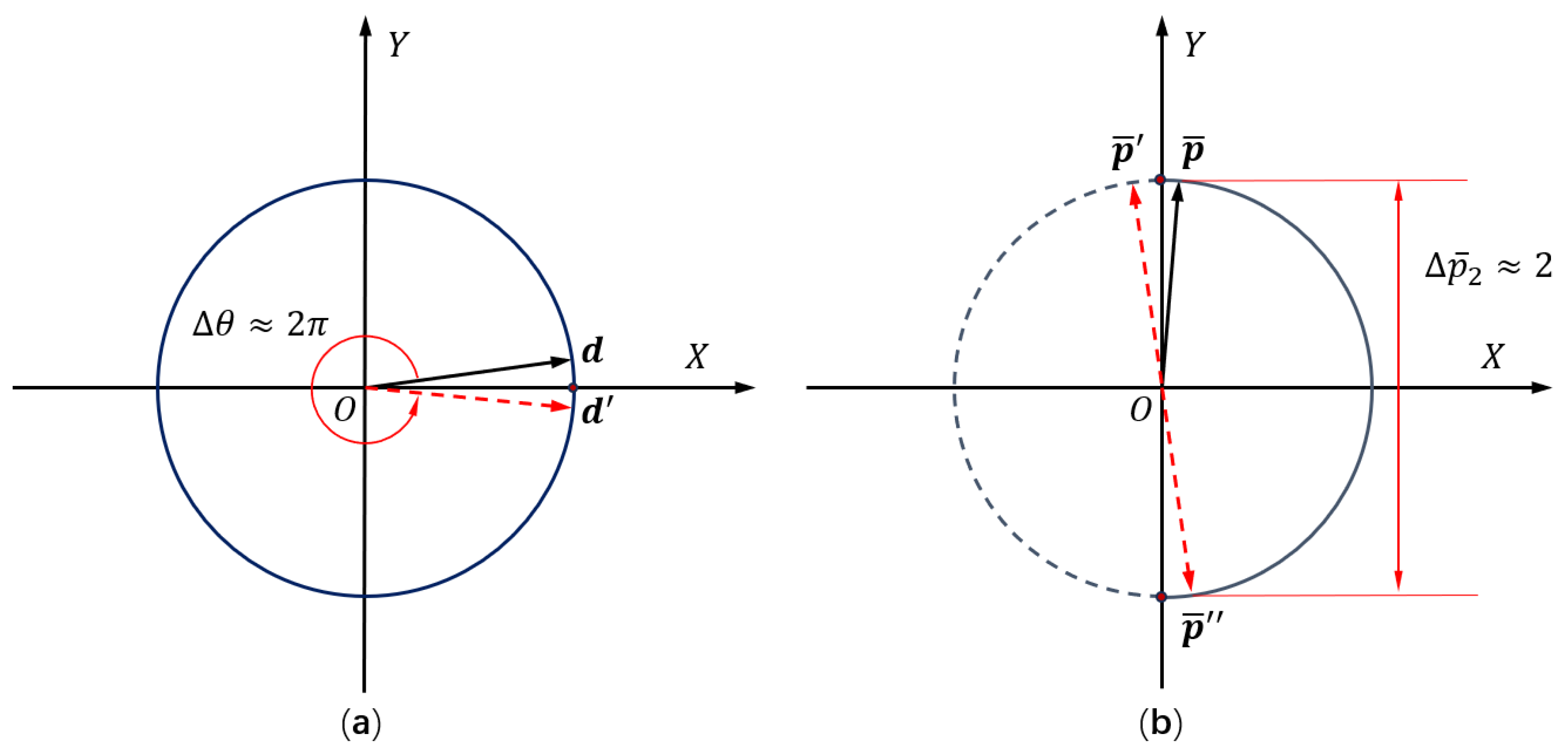
We note that a natural approach to parameterizing the fiber orientations is the polar representation, where a single angular design variable is introduced for each element to define its fiber orientation. While it minimizes the number of design variables, the polar representation introduces a well-documented issue of mathematical discontinuity due to the periodic nature of angles that is often termed " 2 π -ambiguity" [28,36]. As illustrated in Figure 2a, if the angular design variables are bounded within [ 0 , 2 π ] , updating the fiber orientation from a state e near one bound to a state e near the opposite bound requires a change Δ θ 2 π , despite e and e representing nearly identical physical orientations. This introduces nonphysical discontinuities at the design variable bounds, hindering optimization updates. Employing a Cartesian representation provides greater design freedom and mitigates the difficulties associated with the polar representation [28,37], despite doubling the number of design variables per element. Additionally, if the feasible domain is restricted to orientations spanning only 180° (e.g., the right half-circle shown in Figure 2b), a similar discontinuity issue arises. When updating from an orientation e near the boundary to an orientation e just beyond it, the equivalent physical orientation e lies within the feasible domain due to directional symmetry. Thus, the required change Δ p ¯ 2 2 in the design variable remains large, again creating nonphysical gaps that impede updates. Setting design variables ranging in value from 1.0 to 1.0 enables fiber orientations over the entire unit circle. The artificial boundaries and associated discontinuities are thereby eliminated, so this strategy is preferable [29,30,38].

2.2. Material Interpolation Scheme

Fiber-reinforced composite materials exhibit transversally isotropic behavior. This implies a significant enhancement of mechanical properties, such as modulus and strength, along the longitudinal (fiber) axis compared to their values along transverse directions. Conversely, within the plane perpendicular to the fiber direction, the material’s mechanical response is isotropic.
The constitutive relationship governing the material’s stress–strain response in the principal material coordinates is expressed as follows:
σ = D ε
Here, σ and ε denote the stress and strain vectors, respectively, utilizing the Voigt notation, and  D signifies the stiffness matrix. For 2D cases, when the stress and strain vectors are given by σ = [ σ 11 , σ 22 , σ 12 ] T and ε = [ ε 11 , ε 22 , γ 12 ] T , the stiffness matrix can be determined as the inverse of the compliance matrix, as follows:
D = 1 / E 1 v 21 / E 1 0 v 21 / E 1 1 / E 2 0 0 0 1 / G 12 1
In this context, E 1 and E 2 represent the Young’s moduli of the composite material, measured parallel and perpendicular to the fiber directions, respectively. v 21 signifies the Poisson’s ratio, while G 12 denotes the shear modulus. Thus, for 2D applications, the entire set of mechanical properties for the composite material, within its principal material coordinate system, is fully characterized by four independent coefficients: E 1 , E 2 , v 21 , and G 12 .
In the global coordinate system X Y , the stress–strain relationship is defined by the rotated stiffness matrix, as follows: [39]:
D R = T ε T DT ε
where T ε is the strain transformation matrix. Assume that in the global coordinates, the first principal axis of the composite material is aligned with a unit direction vector e 1 = [ l , m ] T ; then, the strain transformation matrix T ε is given as follows [29,38]:
T ε = l 2 m 2 l m m 2 l 2 l m 2 l m 2 l m l 2 m 2
Thus, when the values of l , m are given, the strain transformation matrix T ε can be calculated. Subsequently, the rotated stiffness matrix can be obtained from Equation (8).
In order to penalize intermediate densities, the stiffness matrix of the composite material in element e is formulated as follows:
D e = g ( x ¯ e ) D e 0 ( p ¯ e 1 , p ¯ e 2 )
where D e 0 is derived using Equations (7)–(9). The modified SIMP model is applied [14], though the composite material is transversally isotropic, rather than isotropic. In the modified SIMP model, g ( x ¯ e ) = ϵ + ( 1 ϵ ) x ¯ e p , with  p = 3 and ϵ = 10 6 .

2.3. Minimum Compliance Design Problem Formulation

The finite element equation for a structure subjected to an external load can be expressed as follows:
Ku = f
where f and u represent the global force vector and its corresponding displacement vector, respectively. The global stiffness matrix K is obtained by assembling all element stiffness matrices.
According to Equation (10), the element stiffness matrix k e is calculated as
k e = g ( x ¯ e ) k e 0
where
k e 0 = Ω e B T D e 0 B d Ω
with B being the strain–displacement matrix.
Putting the design variables, objective function, and constraints together, the classical minimum-compliance design problem for composite structures under an external load can be written as follows:
min x , p : c = f T u s . t . : Ku = f e = 1 N v e x ¯ e v f V 0 0 0 x e 1 , 1 e N 1 p e 1 1 , 1 e N 1 p e 2 1 , 1 e N
Here, V 0 and v e denote the volume of the design domain and element e, respectively. v f is the prescribed volume fraction. x and p represent the vectors of density and fiber-orientation design variables, respectively.

2.4. Efficient Solution Method

2.4.1. Finite Element Analysis

When the design domain is discretized with a large number of elements, the topology-optimization problem in (14) becomes computationally demanding due to the nested finite element analysis. However, employing Cartesian grids allows the use of the TSMs-based method, which provides an efficient scheme for performing the finite element computations and significantly speeds up the assembly of the global stiffness matrix [32,33].
For 2D problems, instead of using the Gaussian quadrature technique, the TSMs-based method computes k e 0 in Equation (13) via a linear combination of six TSMs.
k e 0 = n = 1 6 D e , n 0 k t , n 0
where n = i ( i 1 ) / 2 + j and
D e , n 0 = D e , i j 0
k t , n 0 = k e , i i 0 , i = j k e , i j 0 + k e , j i 0 , i > j
Here, D e , i j 0 represents the entry at the ( i , j ) position of the matrix D e 0 . The matrices k e , i j 0 are defined as k e , i j 0 = Ω e B e T D i j B e d Ω , where D i j is a 3 × 3 canonical basis matrix that has an entry of 1 exclusively at its ( i , j ) -th position and zeros elsewhere.

2.4.2. Sensitivity Analysis

Sensitivity analysis is essential in topology optimization for measuring how much each design variable influences the objective and the constraint functions, and it is quite important for design variable updating. When the load is independent of the design, the sensitivity of the structural compliance with respect to an arbitrary design variable α e is expressed as [10] follows:
c α e = u e T k e α e u e
Substituting Equation (12) into Equation (18) yields
c x ¯ e = g ( x ¯ e ) u e T k e 0 u e
c p ¯ e i = g ( x ¯ e ) u e T k e 0 p ¯ e i u e , i = 1 , 2
According to Equation (15), we have
k e 0 p ¯ e i = n = 1 6 D e , n 0 p ¯ e i k t , n 0 , i = 1 , 2
Inserting Equation (21) into (20) yields
c p ¯ e i = g ( x ¯ e ) ( n = 1 6 D e , n 0 p ¯ e i u e T k t , n 0 u e ) , i = 1 , 2
The sensitivity term D e 0 / p ¯ e i in Equation (22) is computed analytically based on Equations (8) and (9), as well as the chain rule of differentiation.
The fiber orientations have no influence on the material amount; thus, the sensitivity of the volume fraction to the fiber orientations is always zero. The sensitivity of the volume fraction to the physical density variables can be explicitly determined, and its derivation will not be given here for brevity.
Once the sensitivities of the objective and constraint functions with respect to physical design variables are established, their sensitivities concerning original design variables can be derived. The derivation for density variables is straightforward; readers may consult [14] for further information.
For orientation variables, the sensitivity of the objective function with respect to the filtered orientation variables can be readily found using the chain rule of differentiation, as follows:
c p ˜ e 1 c p ˜ e 2 = p ¯ e 1 p ˜ e 1 p ¯ e 2 p ˜ e 1 p ¯ e 1 p ˜ e 2 p ¯ e 2 p ˜ e 2 c p ¯ e 1 c p ¯ e 2
By simple mathematical operation, it can be seen that
p ¯ e 1 p ˜ e 1 p ¯ e 2 p ˜ e 1 p ¯ e 1 p ˜ e 2 p ¯ e 2 p ˜ e 2 = 1 p ˜ e I p ¯ e p ¯ e T
When the sensitivity of the objective function with respect to the filtered orientation design variables is obtained, its sensitivity to the original orientation design variables can be calculated as follows:
c p e i = j N e c p ˜ j i p ˜ j i p e i

2.4.3. Design Variable Update

In minimum-compliance design problems, a single material volume constraint is typically present. Since orientation variables do not influence this constraint, an opportunity arises for efficient update of the design variables in each optimization step. Instead of updating the density and orientation design variables simultaneously using general mathematical programming algorithms such as the Method of Moving Asymptotes (MMA) [40], this work updates the density and orientation design variables separately, which has been shown to be both robust and more efficient, as demonstrated by [41].
The updated density variable x e new is determined using the optimality criteria method [14], as follows:
x e new = max ( 0 , x e m ) if x e B e η max ( 0 , x e m ) min ( 1 , x e + m ) if x e B e η min ( 1 , x e + m ) x e B e η otherwise
where m is a move limit, η is a numerical damping coefficient, and  B e is derived from the optimality condition as follows:
B e = c x e λ V x e
The Lagrangian multiplier λ needs to be selected to satisfy the volume constraint. Its appropriate value is typically determined using a bisection algorithm.
For orientation variables, which are bounded rather than subject to general constraints, an explicit convex approximation of the objective function as suggested by [41] is employed. This approach enables the construction of an explicit convex subproblem in each optimization step, as follows:
min p : f ( p ) = f 1 ( p 1 ) + f 2 ( p 2 ) + r 0 s . t . : p e 1 , l p e 1 p e 1 , u , 1 e N p e 2 , l p e 2 p e 2 , u , 1 e N
where
f i ( p i ) = e = 1 N ( P e i U e i p e i + Q e i p e i L e i )
and r 0 is a constant that is dependent only on the current design. The expressions of P e i , Q e i , U e i and L e i can be found in [42]. To mitigate overly large step sizes during optimization, bounds are imposed on the orientation variables.
The subproblem formulation (28) separates the approximated objective function, resulting in independent subproblems subject only to bound constraints. By leveraging this separability, we can analytically determine the optimum solution for each subproblem as follows [33]:
p e i s = p e i , l , if p e i * < p e i , l p e i * , if p e i * [ p e i , l , p e i , u ] p e i , u , if p e i * > p e i , u
where
p e i * = P e i L e i + Q e i U e i P e i + Q e i

3. MATLAB Implementation

3.1. Architecture

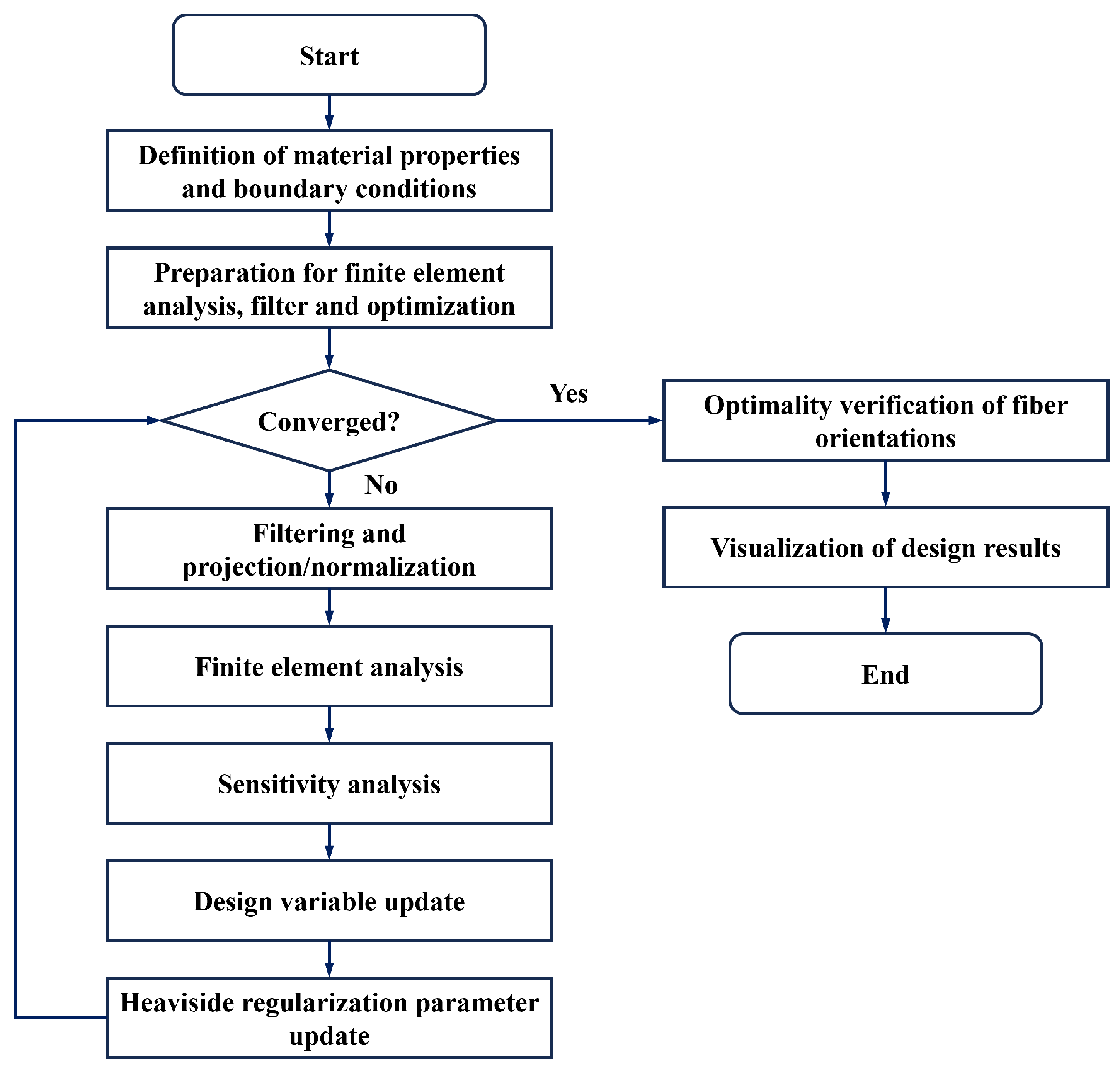
In this section, we introduce CFRCTop, the MATLAB implementation for efficient topology optimization of CFRCs. The implementation of CFRCTop follows the flowchart shown in Figure 3 and employs modular design principles. Its source code comprises ten distinct files, with each encapsulating specific functional components to facilitate maintainability. The complete MATLAB code is provided in the Supplementary Materials and is also available at https://github.com/qmdxcube/CFRCTop (accessed on 20 August 2025).
The file CFRCTop.m constitutes the primary computational framework. It integrates three core functionalities: (1) definition of the optimization problem, (2) solution of the optimization problem, and (3) visualization of optimized designs. During each optimization iteration, the computational sequence initiates with the calculation of the physical density and fiber-orientation fields. Then, finite element analysis, sensitivity analysis, and design variable updating are conducted sequentially. To promote convergence towards a crisp, near-binary material distribution, the value of the Heaviside projection parameter β is progressively increased during the optimization process. Upon completion of the optimization iterations, the converged structural topology, represented by the physical density field, and the optimized fiber orientations, represented by the physical direction vectors, are visualized to illustrate the final design configuration.
The code is executed in the MATLAB environment using the following command:
CFRCTop(nelx,nely,he,thickness,volfrac,rmin,rmin_p)
where nelx and nely represent the number of elements in the horizontal and vertical directions, respectively; he is the element size; thickness is the thickness of the design domain; volfrac is the prescribed volume fraction; rmin and rmin_p are the filter radii of for the density and orientation fields, respectively, and they represent dimensionless quantities defined relative to the element size.
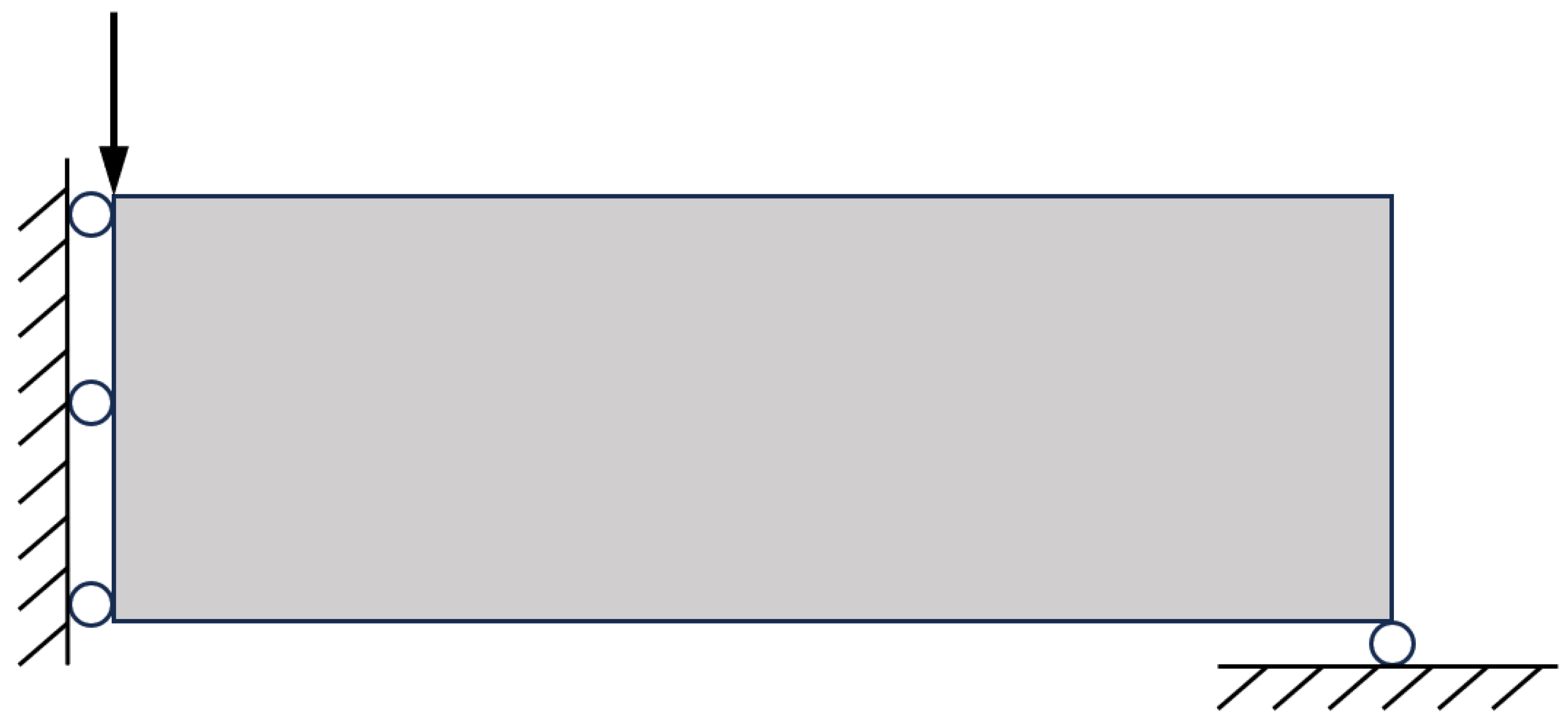
The dimension of the design domain in the horizontal direction is nelx×he, and that in the vertical direction is nely× he. The material properties of the composite material are specified in lines 2–4, where the values of four independent parameters E1,E2,v21, and G12 are given. The stiffness matrix for the composite when its first principle axis is aligned with the horizontal axis is calculated in line 4, corresponding to Equation (8). The boundary conditions are defined in lines 5–11. The classic Messerschmitt–Bölkow–Blohm (MBB) beam problem is considered in default. As shown in Figure 4, only half of the design domain is considered, and the corresponding symmetric boundary conditions are enforced.

3.2. Finite Element Analysis

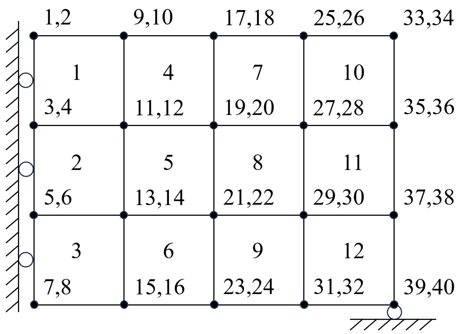
The design domain is meshed into square elements. As illustrated in Figure 5, a coarse example mesh features 12 elements, with each element possessing four nodes and two degrees of freedom (DOFs) per node. A consistent column-wise numbering scheme is applied to both the nodes and the elements. Under this scheme, for any given node n, its horizontal and vertical displacements are assigned degrees of freedom (DOFs) 2 n 1 and 2 n , respectively.
For finite element analysis, most of the procedures are the same as those developed in top88. The main difference is how to compute element stiffness matrices. Because the properties of the composite material depend on the fiber orientation, in each optimized step, the local elasticity matrix for the composite material is first computed in line 69. Then, a material interpolation scheme is applied to determine the effective elastic properties for each element in line 70. According to the TSMs-based method, the element stiffness matrices can be obtained by linear combinations of six TSMs; then, the sK for assembling the global stiffness matrix is computed directly in lines 71–78. Note that these six TSMs are the same for all elements; thus, they are precomputed in lines 19–31 prior to the optimization loop. The assembly of the global stiffness matrix, which is done in line 79, is accelerated via vectorized operations inspired by the top88 methodology. iK and jK are prepared in lines 13–18 prior to the optimization loop. When the global stiffness matrix is ready, the finite element equations are solved in lines 80–82. When the displacement field is obtained, the structural compliance and current volume fraction are evaluated in lines 83–84.
Noting that to ensure generality and simplicity, the computation of the element stiffness matrix is achieved by a function encapsulated in BasicKe.m. This facilitates the implementation of the TSMs because the difference in their computation is attributed only to the DT in lines 25–27. Additionally, the material interpolation is also encapsulated in a function in MaterialInterpolation.m. Here, the modified SIMP interpolation is used. However, any other interpolation schemes can be applied as well.

3.3. Filtering and Projection/Normalization

According to the theory fundamentals described in Section 2.1, both the density and fiber-orientation fields employ a three-field representation scheme. For the density variables, these comprise the original density field x, the filtered density field xTilde, and the physical density field xPhys. Similarly, the fiber-orientation field consists of the original fiber-orientation field px and py, the filtered orientation field pxTilde and pyTilde, and the physical orientation field pxPhys and pyPhys. These variables are defined in lines 33–41.
The implementation of the filters also follow the practice in top88 and top110. The H and Hs are precomputed in line 43 for the density design variables, while the Hp and Hps for the fiber-orientation design variables are precomputed in line 44. The computation of these matrices is achieved by invoking the function in PreFILTER.m. Note that the filter for the density design variables and that for the fiber-orientation variables can have different filter radii. When the filtered variables xTilde, pxTilde, and pyTilde are computed, the physical density field xPhys is computed in line 63 by the smoothed Heaviside projection, while the physical orientation fields pxPhys and pyPhys are computed in lines 64–65 by normalizing pxTilde and pyTilde.

3.4. Sensitivity Analysis

Sensitivity analysis is performed subsequent to obtaining the finite element solution. Within lines 85–105, partial derivatives of the compliance objective are analytically computed concerning the physical density variables xPhys and physical fiber-orientation variables (pxPhys, pyPhys). These sensitivities are then back-propagated through the projection/normalization and filtering operations to obtain gradients with respect to the original design variables in lines 106–126. Note that the pagemtimes function of MATLAB is used to compute matrix products for corresponding pages of 3-D input arrays, eliminating the need for explicit loops over array dimensions. The volume-constraint sensitivity is calculated solely with respect to the density variables, as it remains independent of fiber orientation.

3.5. Design Variable Update

The design variables are updated using distinct strategies: the density variables are updated via the OC method, while the fiber-orientation variables are updated using the MMA algorithm for unconstrained problems.
The OC method for density variables is provided in updateDensityVariables.m, while the MMA method for the fiber-orientation design variables is provided in updateOrientationVariables.m. The implementation of the latter is borrowed from PolyDyna [43]. Since the fiber orientation has no influence on the volume fraction, only bound constraints need to be considered when updating the fiber-orientation design variables. This simplifies optimization algorithm design because no other general constraints are needed. As demonstrated in [41], the separation update of the density and fiber-orientation variables yields the same results but higher efficiency.

3.6. Postprocessing

The files plotDesign.m and plotHistory.m contain the code for postprocessing. The former function visualizes the optimized topology and fiber orientations, while the latter plots the iteration histories of compliance and volume fraction. The plotDesign.m code is inspired by the work of [12]. To visualize the fiber-orientation field, a short line is plotted at the center of each element to indicate its fiber orientation. This is achieved by using the quiver function in MATLAB. For consistency with the density field, fiber orientations are annotated exclusively in elements with density values greater than 0.5.

3.7. Optimality Verification of Fiber Orientations

For the topology optimization of CFRCs, verifying the optimality of the optimized design is a critical concern. Several criteria, including stress-based and strain-based methods [34], have been proposed for predicting the optimal orientation of orthotropic materials. Given that fiber-reinforced composites are typically ’weak’ in shear, according to the results published in [34], the optimal fiber orientation should align with the dominant principal stress direction at every point for minimum-compliance design problems under a single load case. This principle has been widely adopted to determine optimal fiber orientations during iterative optimization steps in numerous studies [5,44,45]. However, as this conclusion is strictly valid only for single-load-case minimum-compliance problems, the present work employs it solely for verifying the optimality of the optimized fiber orientations, not for determining them. As detailed in Section 3.5, fiber orientations are updated based on design sensitivities and explicit convex subproblem formulations, making the proposed method applicable to a broader range of problems.
The optimality verification is implemented in the file verifyOptimality.m. This function efficiently computes the strain at the centroid of each element using vectorized operations. The corresponding stress is then calculated using the element’s rotated stiffness matrix. Subsequently, the principal stress directions for each element are determined by solving the standard eigenvalue problem for the stress tensor. A collinearity metric defined as the absolute value of the inner product of the fiber orientation and the dominant principal stress direction is introduced for each element. A collinearity value approaching unity indicates near-perfect alignment of the fiber orientation with the dominant principal stress direction. Finally, the collinearity values across all elements are visualized to assess global alignment. For consistency with the density-based representation, collinearity values are annotated only for elements with a density exceeding 0.5.

3.8. Results

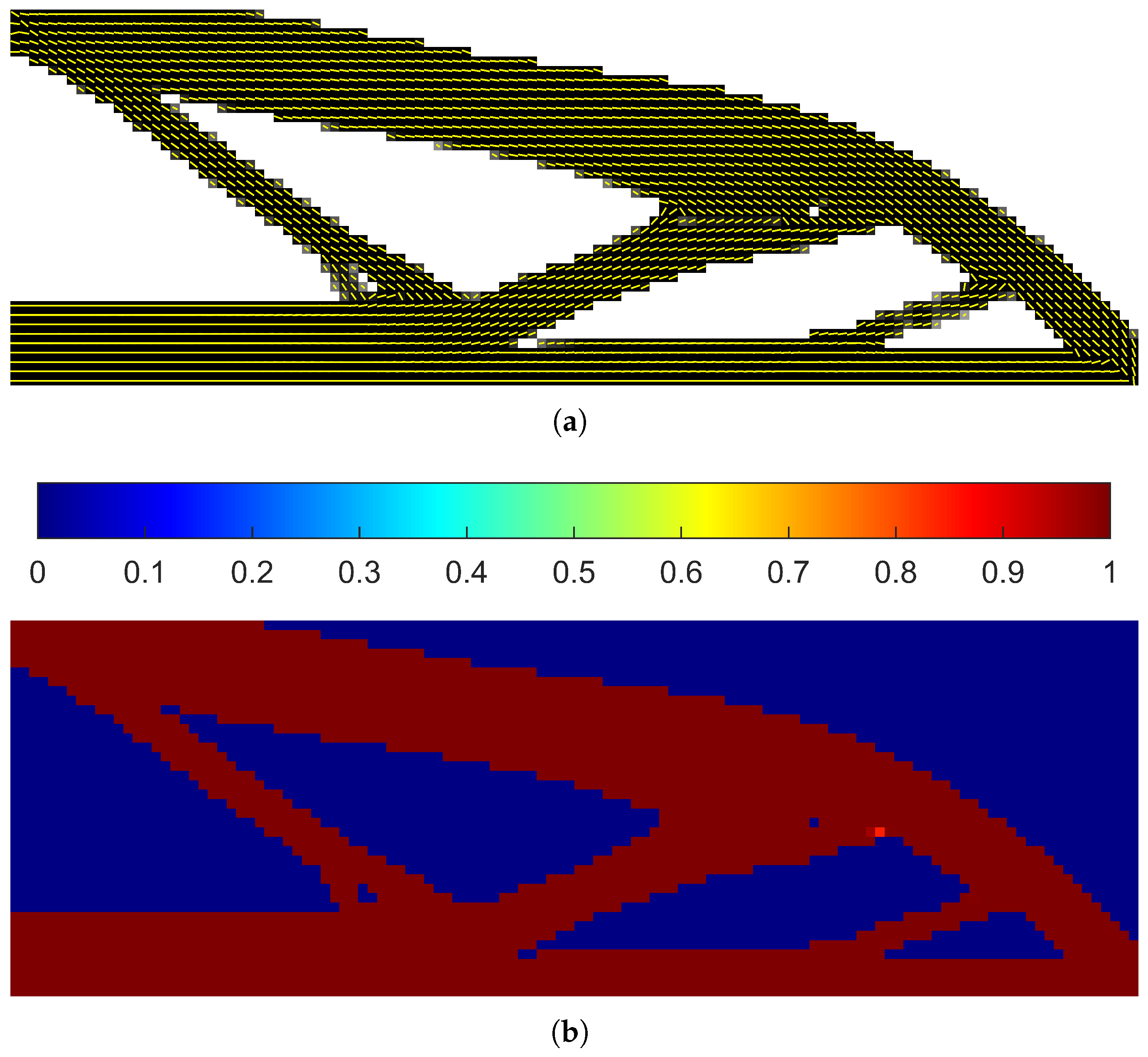
The CFRCTop code is used to optimize the MBB beam with continuous fiber-reinforced composite. The design domain is meshed into 120 × 40 elements, with a volume constraint of 50 % . The filter radii for both the fiber-orientation field and density field are established at twice the element size. Initially, the fiber orientation in all elements aligns with the horizontal axis. The element size and the thickness of the design domain are set to 0.05 and 0.005, respectively.
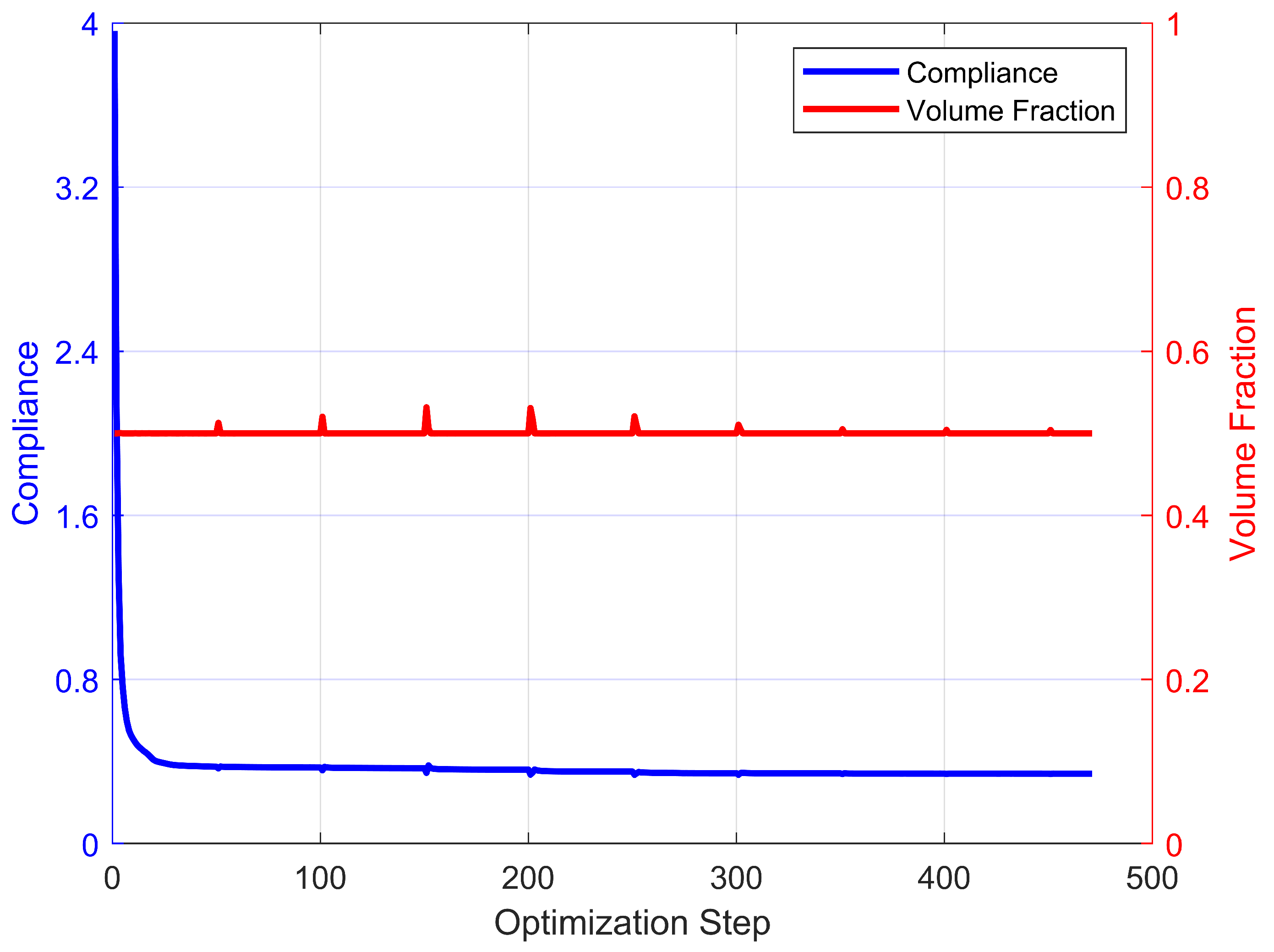
By invocation of the command CFRCTop(120,40,0.05, 0.005,0.5,2.0,2.0), the optimized topology and fiber orientation shown in Figure 6a are obtained. The collinearity of fiber orientations with the dominant principal stress directions is plotted in Figure 6b. The iteration histories of the compliance and volume fraction are plotted in Figure 7. The optimized compliance of the corresponding design is 0.3411. It can be clearly seen from Figure 6a that the fiber orientations vary smoothly in the optimized design and follow the load path, demonstrating the rationality of the optimized topology and fiber orientations. The collinearity plot in Figure 6b confirms the alignment of the fiber orientations with the dominant principal stress direction, further verifying the validity of the optimized design. It should be noted that the occasional jumps observed in the volume fraction iteration history can be attributed to increases in the Heaviside projection parameter.
In order to demonstrate the advantage of concurrently optimizing the topology and fiber orientations, a MATLAB program, CFRCTop_Sequential.m, was also developed. In this program, the topology and fiber orientations are optimized sequentially. First, the topology of the structure is optimized with fixed fiber orientations;  then, the fiber orientations are optimized based on the resulting topology. Because the topology and fiber orientations are optimized separately, it is expected that the obtained design will have worse performance than the design obtained using CFRCTop.m for the same problem.
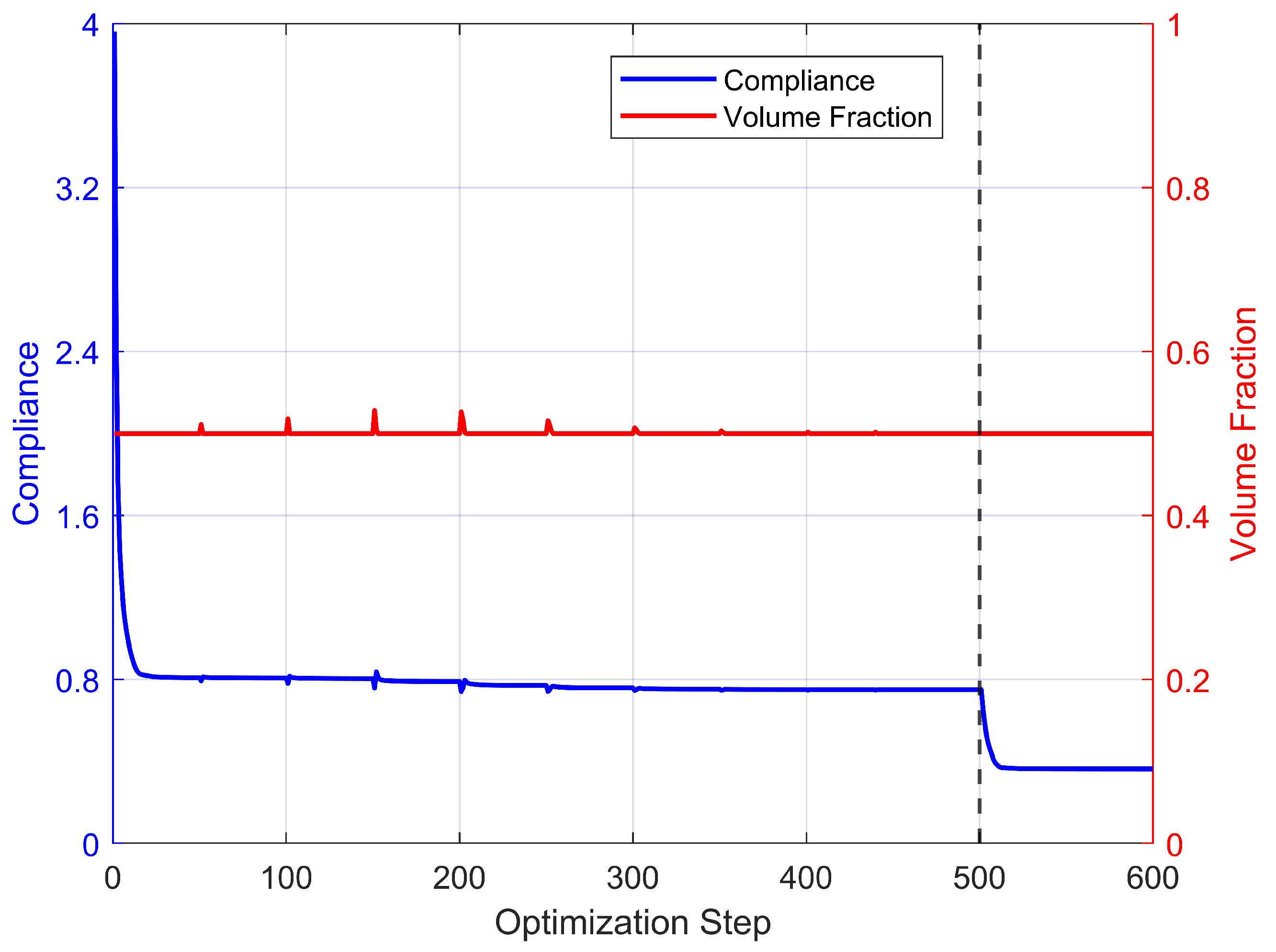
The optimized design obtained using sequential optimization is shown in Figure 8a, and it is clearly different from the design in Figure 6a. The iteration histories for compliance and volume fraction are plotted in Figure 9. In the first stage, the topology is optimized with all fiber orientations aligned horizontally, while in the second stage, the fiber orientations are optimized using the topology from the first stage. The optimized compliance values obtained from the first and second stages are 0.7510 and 0.3640, respectively. The collinearity plot in Figure 8b also verifies the optimality of the fiber orientations from the second stage. It is worth noting that the optimized compliance of the concurrent design is 0.3411, which is smaller than that of the sequential design, thereby demonstrating the advantage of the concurrent design method.

4. Extensions

The top88 code, designed for topology optimization with isotropic materials, details the method for incorporating various boundary conditions, multiple load cases, and passive elements. Since the CFRCTop code is inherited form the top88, its extension to address these issues are straightforward. In this section, some extensions are discussed.

4.1. Different Initialization of the Fiber Orientations

Prior research [33,46] indicates that how initialization of fiber orientation significantly impacts the optimized design of CFRCs. To alter how fiber orientations are initialized, simply adjust lines 34 and 35. The current default has all elements’ fiber orientations oriented along the horizontal axis. In order to change the fiber orientations to aligned them with the vertical axis, the only necessary change is a modification of lines 34 and 35 as follows:
Applsci 15 09242 i001 For the case of random initialization, just make the following change:
Applsci 15 09242 i002
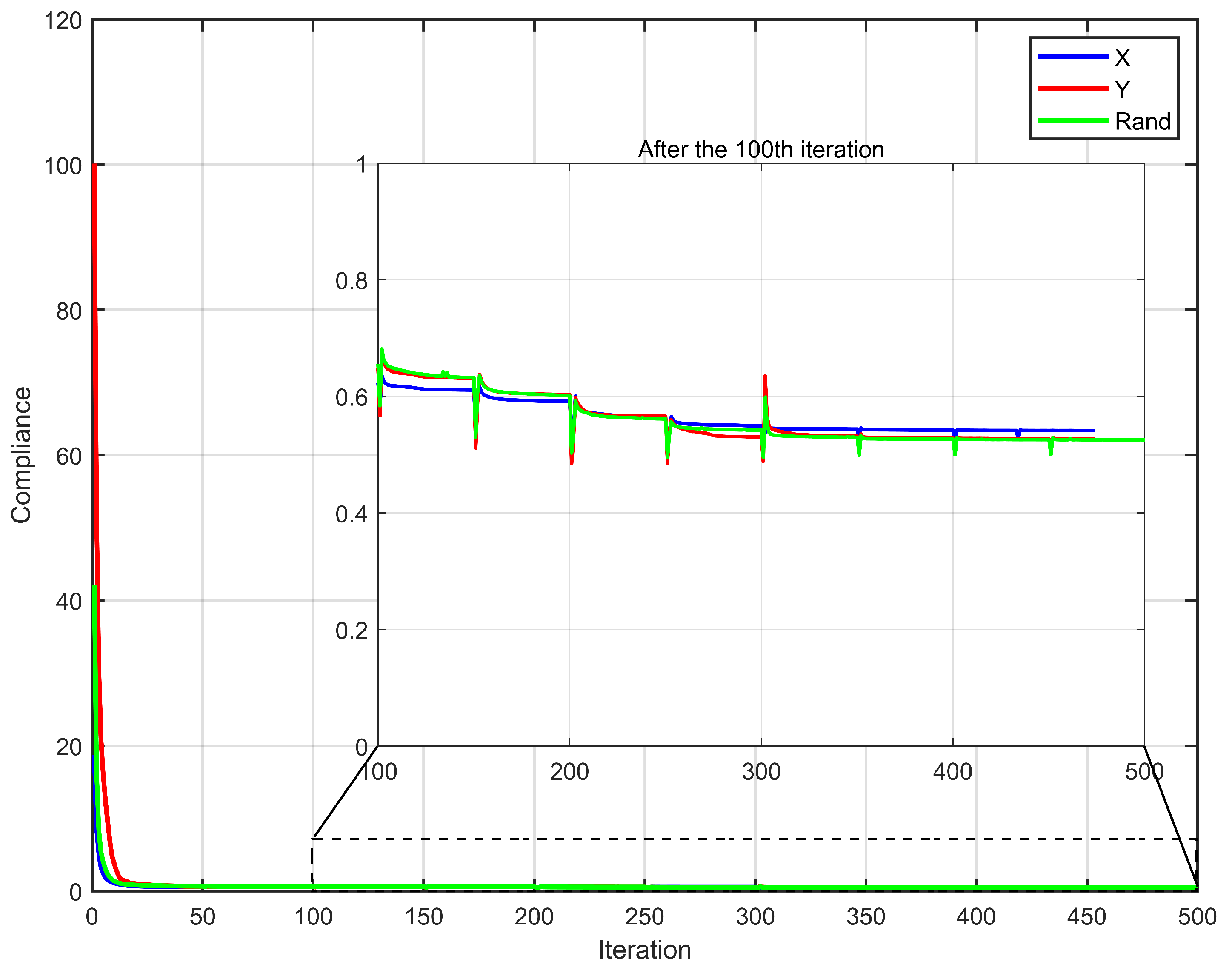
For the MBB problem, the optimized designs obtained from different initializations of the fiber orientations using the function call CFRCTop(150,50,0.05,0.005,0.3,2.0,2.0) are shown in Figure 10. The optimized compliance values of the corresponding designs are 0.5413, 0.5271, and 0.5255, respectively. Even though the optimized designs may be quite different depending on their initialization, their compliance values are typically very close. In this case, the relative difference is within 3 % . The collinearity plots again verify the optimality of the optimized fiber orientations for the three cases. The iteration history of compliance and volume fraction for the three cases are plotted in Figure 11. It can be seen that while the initial fiber orientations may have substantial influence on the initial compliance, the optimized compliance values are very close. According to the suggestion given in [46], random initialization of the fiber orientations may partially avoid poor-quality local minima, so it is recommended in practice. In the following examples, for the purpose of replication, the initial fiber orientations remain aligned with the horizontal direction.

4.2. Other Boundary Conditions

In order to solve other design problems, different boundary conditions need to be enforced. It is worth noting that adjusting the boundary conditions is quite straightforward, as the displacement and load conditions are defined in lines 9 and 11, respectively. For example, solving the short cantilever example (Figure 12) requires only changing line 9 to the following:
Applsci 15 09242 i003 At the same time, line 11 must be changed as follows:
Applsci 15 09242 i004
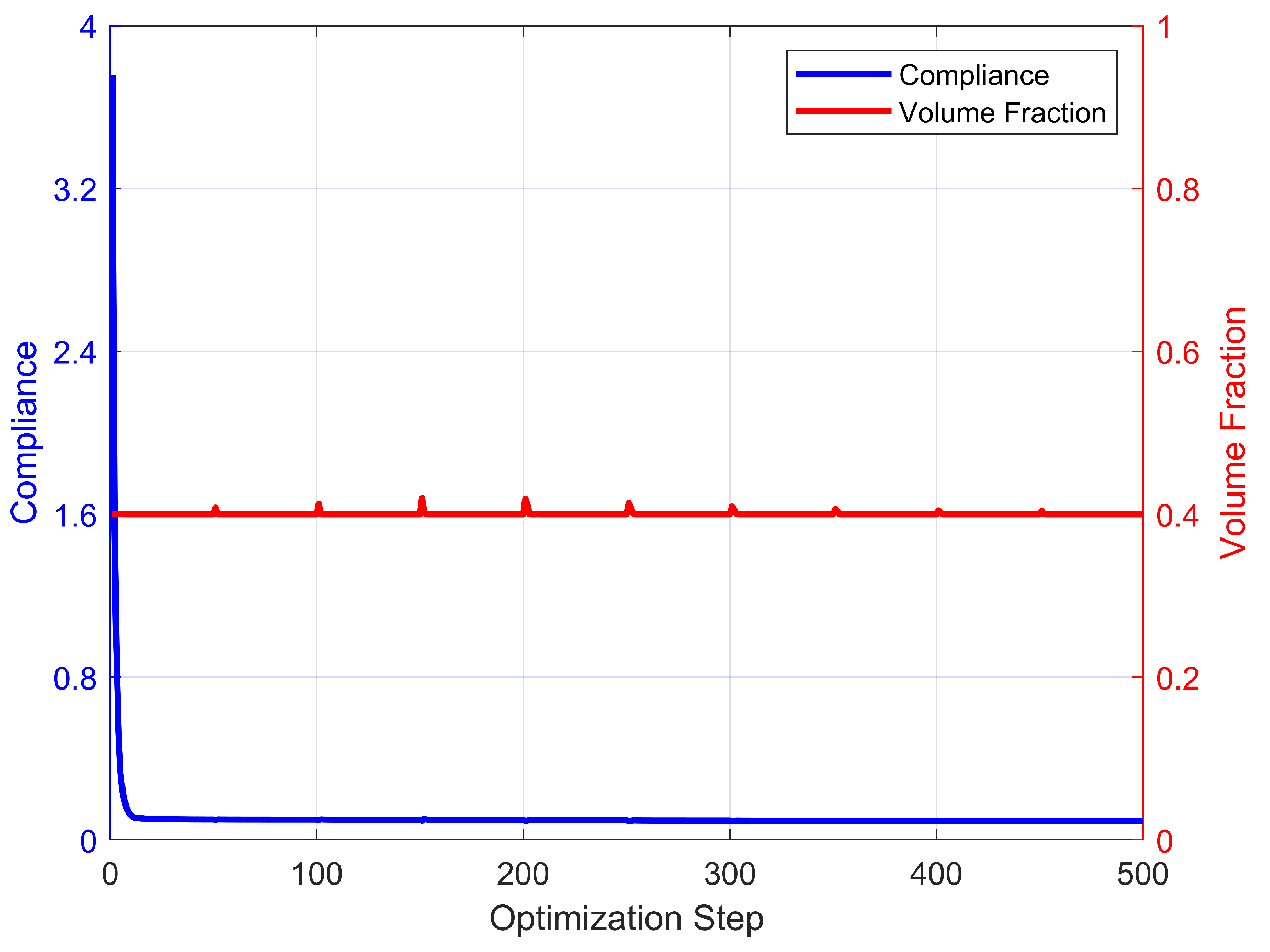
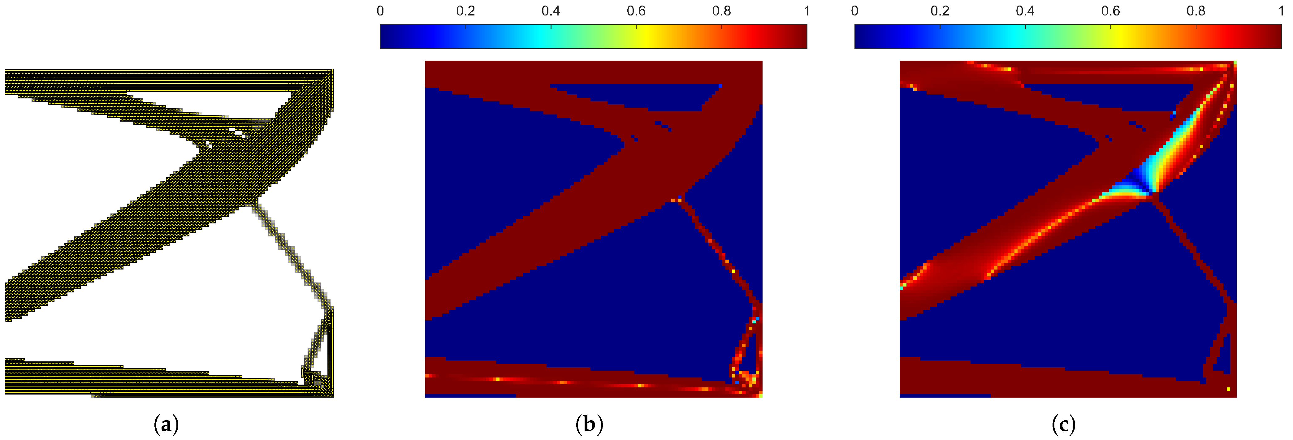
With these changes, the function call CFRCTop(160,100,0.05,0.005,0.4,3.0,3.0) leads to the optimized design in Figure 13. The collinearity plot verifies the optimality of the fiber orientations. The iteration histories of the compliance and volume fraction shown in Figure 14 demonstrate the effectiveness of the code.

4.3. Multiple Load Cases

Extending the code to account for multiple load cases is also very straightforward. Considering the problem given in Figure 15, there are two load cases; thus, the load and displacement vectors should be defined as two-column vectors. Lines 11 and 12 need to be changed as follows:
Applsci 15 09242 i005
The displacement constraints remain consistent with those in the prior example. The solution of the finite element equations for both load cases can be achieved by simply changing line 82 as follows:
Applsci 15 09242 i006
In the case where there are two load cases, the objective function is the sum of the compliance of the structure under two load cases, respectively. Lines 90-102 thus should be replaced by the following codes:
Applsci 15 09242 i007
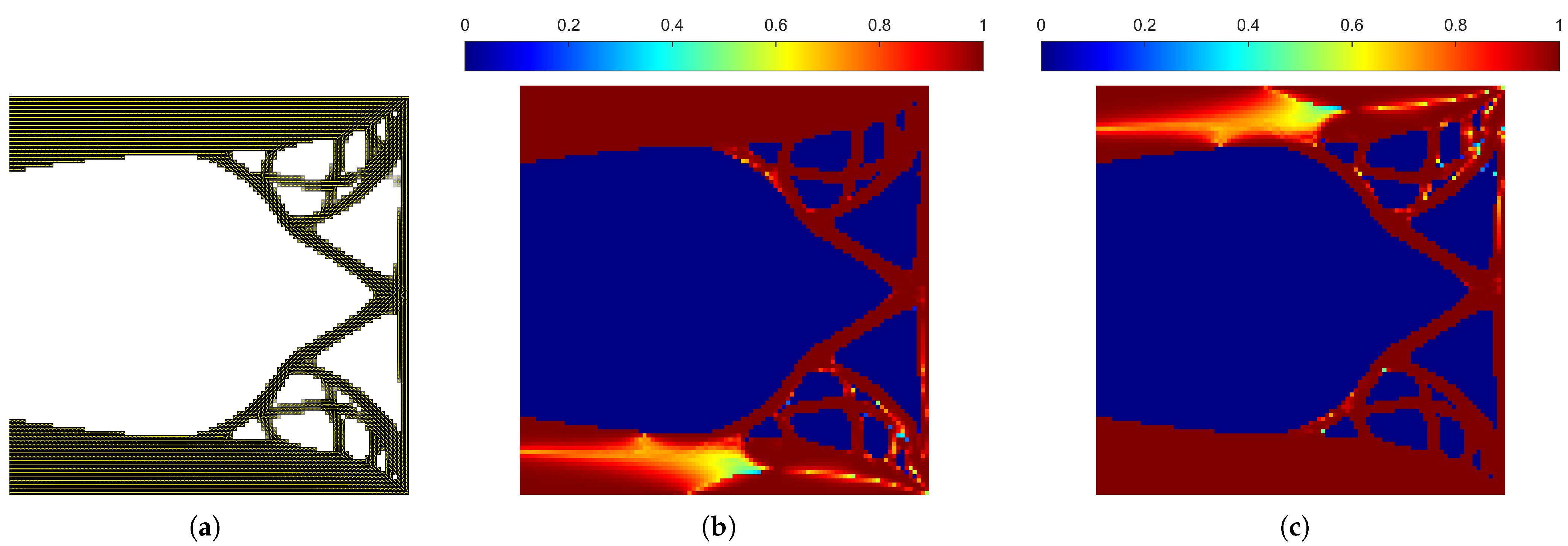
The command CFRCTop(100,100,0.05,0.005,0.4,2.0,2.0) yields the optimized design shown in Figure 16a. The collinearity of the fiber orientations with the dominant principal stress directions under two load cases is shown in Figure 16b and Figure 16c, respectively. Surprisingly, the fiber orientations align with the principal directions almost everywhere under both load cases. However, this is generally not the expected outcome.
When changing the load direction for the second load case to the horizontal direction by modifying the code as follows:
Applsci 15 09242 i008
The optimized design and collinearity of fiber orientations with the dominant principal stress directions under two load cases are shown in Figure 17. Clearly, in this case, the fiber orientations are not aligned with the principal stress direction in many elements, particularly under the second load case.
When the load direction is further changed in both load cases to the horizontal direction, the code is modified as follows:
Applsci 15 09242 i009
The optimized design and collinearity of fiber orientations with the dominant principal stress directions under two load cases are shown in Figure 18. It can be observed that the fiber orientations are not aligned with the principal stress direction in many elements for either load case, again demonstrating that the principal stress directions are not always optimal for fiber orientations.

4.4. Passive Elements

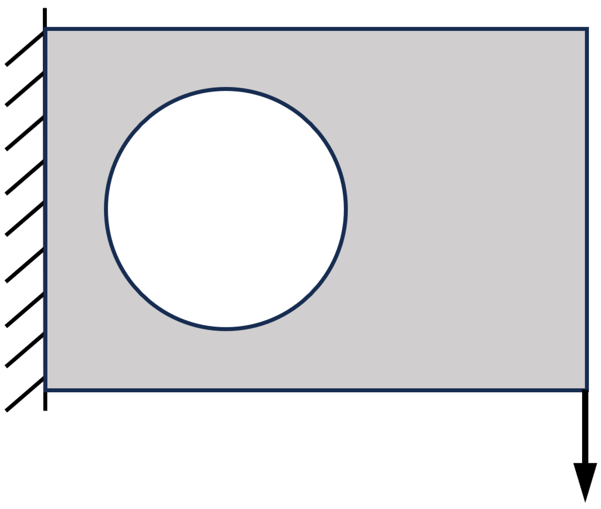
Sometimes, specific regions of the design domain must be designated as either solid or void. This requirement can be accomplished through the use of passive elements. For each element, a variable is assigned to indicate its status. We can use 1 for void and 2 for solid; other values indicate that the corresponding element is free for design. Consider the short cantilever design problem in Figure 19. Here, the circular area within the design domain (with a radius of nely/3 and centered at (nely/2,nelx/3) is designated as void. The displacement and load conditions are the same as those in Figure 12.
In order to indicate the status of each element in the design domain, a nely × nelx matrix passive is defined. For those elements in the circular area, the value is assigned to be 1. Before the optimization loop begins in CFRCTop.m, the following lines need to be inserted.
Applsci 15 09242 i010
At the same time, insert the following lines between lines 64-65:
Applsci 15 09242 i011
Further, the code for the OC update also needs to be modified accordingly.
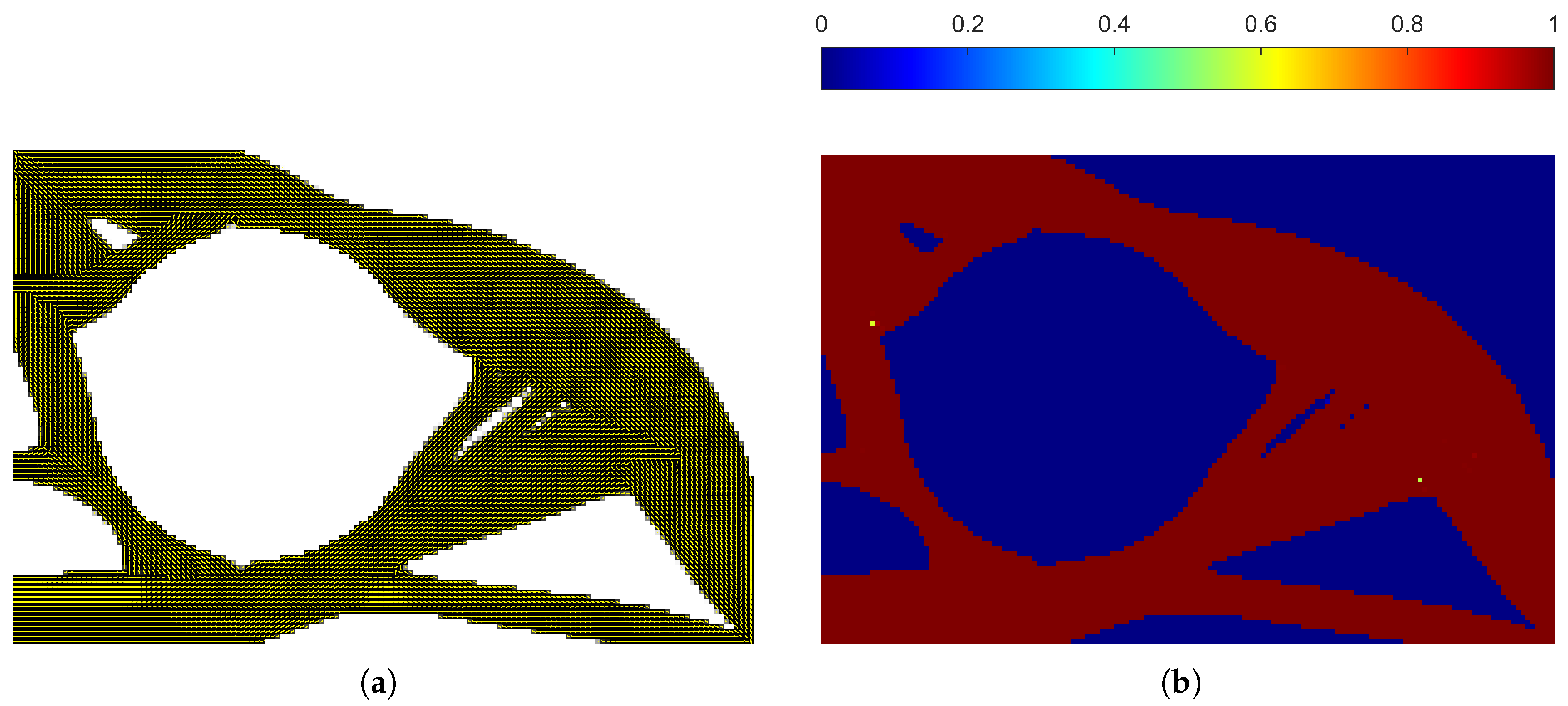
With these changes, the function call CFRCTop(150,100,0.05,0.005,0.5,3.0,3.0) yields the optimized design in Figure 20. The collinearity plot verifies the optimality of the optimized fiber orientations.

5. Computational Performance and Scalability

In this section, we study the computation performance and scalability of the CFRCTop code by solving the MMB problem again, this time for both CFRCs and isotropic materials. For the isotropic case, we use the code Top, which a modification of the top88 code, designed to solve a broader range of problems while retaining the computational efficiency of top88.
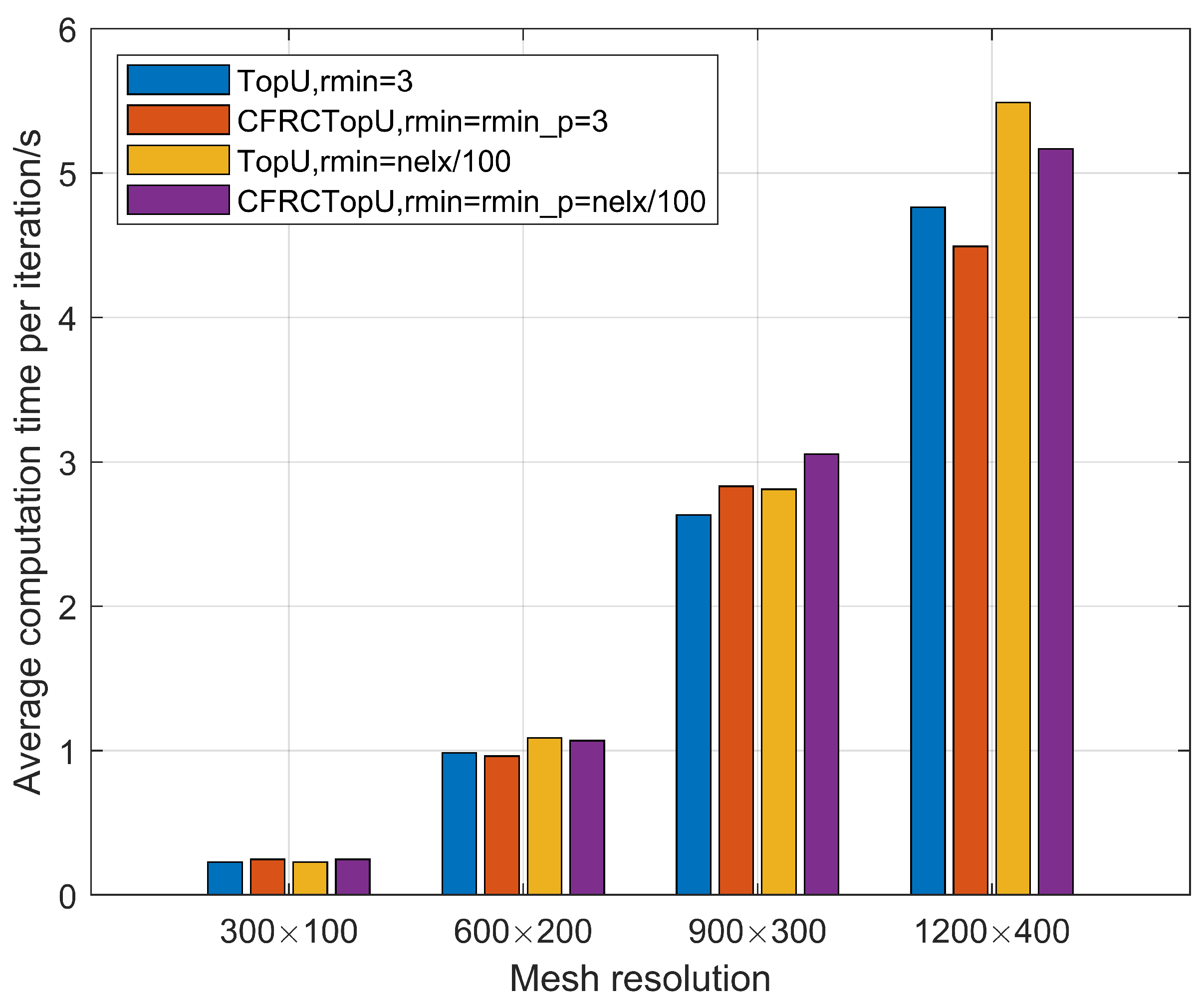
We consider problems with different mesh resolutions. Specifically, four resolutions, 300 × 100 , 600 × 200 , 900 × 300 , and  1200 × 400 , are tested. On this basis, we distinguish two cases. In the first case, both rmin and rmin_p are set to 3.0, while in the second case, both are set to nelx/100. For each case, the maximum number of iterations is set to 100.
The tests were run on a HP OMEN laptop with an Intel(R) Core(TM) i9-12900HX @2.40 GHz CPU, 32 GB of RAM, and MATLAB R2022a running on the Windows 11 Home operating system.
The average computation time per iteration are displayed in Figure 21. The breakdowns of the computation time for all cases are listed in Table 1 and Table 2. It can be seen that the average computation time per iteration is comparable for Top and CFRCTop when they are solving the problem with the same mesh resolution and same filter radius. The time values listed in Table 1 demonstrate that the average computation time for assembly of a global stiffness matrix in CFRCTop increases by only around 50 % compared to Top. This is notable because the former requires the superposition of six TSMs, while the latter needs only one. The reason for this modest increase is that when vectorized operations are used, the generation of the global stiffness matrix by lines 82-83 of CFRCTop takes more time than the computation of all element stiffness matrices. Consequently, the global stiffness generation process dominates the total assembly time.
Surprisingly, the average computation time needed to solve the equilibrium equation is lower in CFRCTop than in Top, which is the main reason why the average computation time per iteration of CFRCTop can be shorter than that of Top. It is worth noting that when a larger filter radius is used for the same resolution, the filtering operation requires more time. Consequently, the updating of the density design variables takes much more computation time because the filtering operation is performed multiple times in a single OC update. It should be noted that because the fiber-orientation design variables are updated separately by an analytical solution and no filtering operation is involved, the updating of the fiber-orientation design variables adds little computational time.
In order to enhance computational efficiency for problems involving a large filter radius, at least three approaches can be applied. The first involves applying the MMA [40] for density variable updates. This methodology requires only a single density filtering computation per optimization iteration, thereby substantially reducing the overall computational time. The second involves accelerating the convergence of the OC method [16], which would reduce the number of filtering operations and the computation time for density design variables. The third approach, which is also the one employed in this section, involves speeding up the filtering operations using alternative implementations. As proposed in [14], the built-in function conv2 is used to perform the filtering operations. The updated versions of Top and CFRCTop that utilize the filter implemented with conv2 are referred to as TopU and CFRCTopU, respectively.
The average computation time per iteration obtained using TopU and CFRCTopU are displayed in Figure 22. The breakdowns of the computation time for all cases are listed in Table 3 and Table 4. It can be seen that because of the speedup of the filtering operations, substantial reduction of the average computation time per iteration is achieved. Even for the resolution of 1200 × 400 , which has about 480,000 elements, the average computation time per iteration is less than 6 s, demonstrating the efficiency of the updated codes.

6. Limitations and Future Directions

Despite the CFRCTop’s high efficiency, it has limitations. For example, the current implementation is designed only to solve minimum-compliance design problems with a single volume fraction constraint, which enables the separate updating of density and fiber-orientation design variables. The implementation can solve only linear elastic problems; when nonlinear problems caused by different tensile and compressive moduli and/or large deformations need to be considered, more advanced algorithms must be developed. The section below outlines some potential future directions.
3D problems: The CFRCTop code is currently designed only to solve 2D plane stress problems. While the extension to 3D problems is conceptually straightforward, it is more computationally complicated. The Cartesian parameterization can still be employed to represent the spatially varying fiber orientations [30]. In addition, the nested finite element analysis will become time-consuming and dominate the total computation time. In such cases, the techniques proposed in [16] can be used to further accelerate the assembly process of the global stiffness matrix, while the multigrid preconditioned conjugate gradient (MGPCG) method [47] can be employed to accelerate the solving of the equilibrium equation.
Plate and shell problems: In practical engineering, composite parts are usually made in the form of a plate or shell structure. For the optimal design of plate or shell structures, an important challenge is the consideration of lamination parameters and through-thickness property variations, which introduce a higher degree of design freedom and complexity compared to 2D plane stress problems. Optimal design of variable-stiffness composite structures can be implemented using lamination parameters [48] or polar parameters [49].
Varying fiber content: In this work, the fiber content is assumed to be constant and the mechanical properties are given directly. Additive manufacturing techniques, however, allow the fabrication of designs with varying fiber content. For this type of problem, the equivalent mechanical properties of composite materials with different fiber contents can be computed analytically or experimentally [50,51]. Therefore, only one additional design variable per element needs to be introduced to represent the fiber content in that element. All parts of the current code can be readily extended to solve such optimization problems, with the exception that more advanced optimization algorithms, such as the MMA [40] algorithm, are needed to update the design variables.
Manufacturing constraints: Despite the fact that advanced manufacturing techniques can virtually fabricate designs of any geometry and fiber orientation, they also impose some constraints on the design. Therefore, it is necessary to consider manufacturing constraints in the optimization formulation to ensure that the optimized design can be fabricated. Extensions can be implemented based on the current code and the methods developed in [29,38].

7. Conclusions

This work presents CFRCTop, a MATLAB implementation for topology optimization of continuous fiber-reinforced composite structures. The fundamentals of the theory are reviewed first; then, the MATLAB implementation is introduced. Numerical results validate the effectiveness of the codes. Extensions to other problems are also given.
This code is built upon the famous and efficient topology optimization code top88. Top88 focuses on topology optimization for isotropic materials. In contrast, CFRCTop is tailored for composite materials, where both the material distribution and the fiber orientations significantly influence the structure’s compliance under a specific load. CFRCTop is able to simultaneously optimize the materials’ distribution and fiber orientations.
The implementation of CFRCTop maximizes the utilization of vectorized operations within MATLAB; thus, the code is very efficient. The implementation also follows the philosophy of modular design. Consequently, it can be used to test many new functionalities, such as material interpolation schemes and methods for updating design variables.
In the future, CFRCTop will be extended to solve more complicated problems, such as varying fiber content, manufacturing constraints, and others.

Supplementary Materials

The following supporting information can be downloaded at: https://www.mdpi.com/article/10.3390/app15179242/s1, MATLAB code.

Funding

This research was funded by the National Natural Science Foundation of China grant number 52105240.

Institutional Review Board Statement

Not applicable.

Informed Consent Statement

Not applicable.

Data Availability Statement

The complete MATLAB code is also available at https://github.com/qmdxcube/CFRCTop, accessed on 20 August 2025.

Acknowledgments

During the preparation of this manuscript, the author used DeepSeek R1 for the purposes of language editing. The author has reviewed and edited the output and takes full responsibility for the content of this publication.

Conflicts of Interest

The author declares no conflicts of interest.

References

  1. Tian, X.; Todoroki, A.; Liu, T.; Wu, L.; Hou, Z.; Ueda, M.; Hirano, Y.; Matsuzaki, R.; Mizukami, K.; Iizuka, K.; et al. 3D printing of continuous fiber reinforced polymer composites: Development, application, and prospective. Chin. J. Mech. Eng. Addit. Manuf. Front. 2022, 1, 100016. [Google Scholar] [CrossRef]
  2. Cheng, P.; Peng, Y.; Li, S.; Rao, Y.; Le Duigou, A.; Wang, K.; Ahzi, S. 3D printed continuous fiber reinforced composite lightweight structures: A review and outlook. Compos. Part B Eng. 2022, 250, 110450. [Google Scholar] [CrossRef]
  3. Liu, G.; Xiong, Y.; Zhou, L. Additive manufacturing of continuous fiber reinforced polymer composites: Design opportunities and novel applications. Compos. Commun. 2021, 27, 100907. [Google Scholar] [CrossRef]
  4. Jiang, D.; Hoglund, R.; Smith, D.E. Continuous fiber angle topology optimization for polymer composite deposition additive manufacturing applications. Fibers 2019, 7, 14. [Google Scholar] [CrossRef]
  5. Safonov, A.A. 3D topology optimization of continuous fiber-reinforced structures via natural evolution method. Compos. Struct. 2019, 215, 289–297. [Google Scholar] [CrossRef]
  6. Chen, Y.; Ye, L. Topological design for 3D-printing of carbon fibre reinforced composite structural parts. Compos. Sci. Technol. 2021, 204, 108644. [Google Scholar] [CrossRef]
  7. Zhou, Y.; Nomura, T.; Zhao, E.; Saitou, K. Large-scale three-dimensional anisotropic topology optimization of variable-axial lightweight composite structures. J. Mech. Des. 2022, 144, 011702. [Google Scholar] [CrossRef]
  8. Qiu, Z.; Li, Q.; Luo, Y.; Liu, S. Concurrent topology and fiber orientation optimization method for fiber-reinforced composites based on composite additive manufacturing. Comput. Methods Appl. Mech. Eng. 2022, 395, 114962. [Google Scholar] [CrossRef]
  9. Habashneh, M.; Rad, M.M. Optimizing structural topology design through consideration of fatigue crack propagation. Comput. Methods Appl. Mech. Eng. 2024, 419, 116629. [Google Scholar] [CrossRef]
  10. Bendsøe, M.P.; Sigmund, O. Topology Optimization: Theory, Methods and Applications; Springer: Cham, Switzerland, 2003. [Google Scholar]
  11. Gandhi, Y.; Minak, G. A review on topology optimization strategies for additively manufactured continuous fiber-reinforced composite structures. Appl. Sci. 2022, 12, 11211. [Google Scholar] [CrossRef]
  12. Jiang, S.; Shang, C.; Li, J.; Yi, B.; Peng, X. Topology optimization of anisotropic materials with smooth fiber orientation. Appl. Sci. 2024, 14, 5947. [Google Scholar] [CrossRef]
  13. Sigmund, O. A 99 line topology optimization code written in Matlab. Struct. Multidiscip. Optim. 2001, 21, 120–127. [Google Scholar] [CrossRef]
  14. Andreassen, E.; Clausen, A.; Schevenels, M.; Lazarov, B.S.; Sigmund, O. Efficient topology optimization in MATLAB using 88 lines of code. Struct. Multidiscip. Optim. 2011, 43, 1–16. [Google Scholar] [CrossRef]
  15. Liu, K.; Tovar, A. An efficient 3D topology optimization code written in Matlab. Struct. Multidiscip. Optim. 2014, 50, 1175–1196. [Google Scholar] [CrossRef]
  16. Ferrari, F.; Sigmund, O. A new generation 99 line Matlab code for compliance topology optimization and its extension to 3D. Struct. Multidiscip. Optim. 2020, 62, 2211–2228. [Google Scholar] [CrossRef]
  17. Talischi, C.; Paulino, G.H.; Pereira, A.; Menezes, I.F. PolyTop: A Matlab implementation of a general topology optimization framework using unstructured polygonal finite element meshes. Struct. Multidiscip. Optim. 2012, 45, 329–357. [Google Scholar] [CrossRef]
  18. Giraldo-Londoño, O.; Paulino, G.H. PolyStress: A Matlab implementation for local stress-constrained topology optimization using the augmented Lagrangian method. Struct. Multidiscip. Optim. 2021, 63, 2065–2097. [Google Scholar] [CrossRef]
  19. Wei, P.; Li, Z.; Li, X.; Wang, M.Y. An 88-line MATLAB code for the parameterized level set method based topology optimization using radial basis functions. Struct. Multidiscip. Optim. 2018, 58, 831–849. [Google Scholar] [CrossRef]
  20. Sanders, E.D.; Pereira, A.; Aguiló, M.A.; Paulino, G.H. PolyMat: An efficient Matlab code for multi-material topology optimization. Struct. Multidiscip. Optim. 2018, 58, 2727–2759. [Google Scholar] [CrossRef]
  21. Gao, J.; Wang, L.; Luo, Z.; Gao, L. IgaTop: An implementation of topology optimization for structures using IGA in MATLAB. Struct. Multidiscip. Optim. 2021, 64, 1669–1700. [Google Scholar] [CrossRef]
  22. Du, Z.; Cui, T.; Liu, C.; Zhang, W.; Guo, Y.; Guo, X. An efficient and easy-to-extend Matlab code of the Moving Morphable Component (MMC) method for three-dimensional topology optimization. Struct. Multidiscip. Optim. 2022, 65, 158. [Google Scholar] [CrossRef]
  23. Wang, C.; Zhao, Z.; Zhou, M.; Sigmund, O.; Zhang, X.S. A comprehensive review of educational articles on structural and multidisciplinary optimization. Struct. Multidiscip. Optim. 2021, 64, 2827–2880. [Google Scholar] [CrossRef]
  24. Wang, Y.; Li, X.; Long, K.; Wei, P. Open-source codes of topology optimization: A summary for beginners to start their research. Comput. Model. Eng. Sci. 2023, 137, 1–34. [Google Scholar] [CrossRef]
  25. Zheng, R.; Yi, B.; Peng, X.; Yoon, G.H. An efficient code for the multi-material topology optimization of 2D/3D continuum structures written in MATLAB. Appl. Sci. 2024, 14, 657. [Google Scholar] [CrossRef]
  26. Bendsøe, M.P. Optimal shape design as a material distribution problem. Struct. Optim. 1989, 1, 193–202. [Google Scholar] [CrossRef]
  27. Zhou, M.; Rozvany, G. The COC algorithm, Part II: Topological, geometrical and generalized shape optimization. Comput. Methods Appl. Mech. Eng. 1991, 89, 309–336. [Google Scholar] [CrossRef]
  28. Nomura, T.; Dede, E.M.; Lee, J.; Yamasaki, S.; Matsumori, T.; Kawamoto, A.; Kikuchi, N. General topology optimization method with continuous and discrete orientation design using isoparametric projection. Int. J. Numer. Methods Eng. 2015, 101, 571–605. [Google Scholar] [CrossRef]
  29. Luo, C.; Ferrari, F.; Guest, J.K. Design optimization of advanced tow-steered composites with manufacturing constraints. Compos. Part B Eng. 2024, 284, 111739. [Google Scholar] [CrossRef]
  30. Zhao, J.; Qi, T.; Wang, C. Topology optimization of 3D continuous fiber-reinforced composites using Cartesian parametrization of fiber orientations. Struct. Multidiscip. Optim. 2024, 67, 153. [Google Scholar] [CrossRef]
  31. Kumar, T.; Suresh, K. A density-and-strain-based K-clustering approach to microstructural topology optimization. Struct. Multidiscip. Optim. 2020, 61, 1399–1415. [Google Scholar] [CrossRef]
  32. Chandrasekhar, A.; Mirzendehdel, A.; Behandish, M.; Suresh, K. Frc-tounn: Topology optimization of continuous fiber reinforced composites using neural network. Comput. Aided Des. 2023, 156, 103449. [Google Scholar] [CrossRef]
  33. Zhao, J.; Qi, T.; Wang, C. Efficient GPU accelerated topology optimization of composite structures with spatially varying fiber orientations. Comput. Methods Appl. Mech. Eng. 2024, 421, 116809. [Google Scholar] [CrossRef]
  34. Gea, H.; Luo, J. On the stress-based and strain-based methods for predicting optimal orientation of orthotropic materials. Struct. Multidiscip. Optim. 2004, 26, 229–234. [Google Scholar] [CrossRef]
  35. Bourdin, B. Filters in topology optimization. Int. J. Numer. Methods Eng. 2001, 50, 2143–2158. [Google Scholar] [CrossRef]
  36. Nomura, T.; Kawamoto, A.; Kondoh, T.; Dede, E.M.; Lee, J.; Song, Y.; Kikuchi, N. Inverse design of structure and fiber orientation by means of topology optimization with tensor field variables. Compos. Part B Eng. 2019, 176, 107187. [Google Scholar] [CrossRef]
  37. Lee, J.; Kim, D.; Nomura, T.; Dede, E.M.; Jeonghoon, Y. Topology optimization for continuous and discrete orientation design of functionally graded fiber-reinforced composite structures. Compos. Struct. 2018, 201, 217–233. [Google Scholar] [CrossRef]
  38. Wong, J.; Sanders, E.D.; Rosen, D.W. Topology optimization of additively manufactured continuous fiber-reinforced structures with constraints on fiber path geometry. Struct. Multidiscip. Optim. 2025, 68, 87. [Google Scholar] [CrossRef]
  39. Kubalak, J.R.; Wicks, A.L.; Williams, C.B. Investigation of parameter spaces for topology optimization with three-dimensional orientation fields for multi-axis additive manufacturing. J. Mech. Des. 2021, 143, 051701. [Google Scholar] [CrossRef]
  40. Svanberg, K. The method of moving asymptotes¡ªa new method for structural optimization. Int. J. Numer. Methods Eng. 1987, 24, 359–373. [Google Scholar] [CrossRef]
  41. Zhang, X.S.; Chi, H.; Zhao, Z. Topology optimization of hyperelastic structures with anisotropic fiber reinforcement under large deformations. Comput. Methods Appl. Mech. Eng. 2021, 378, 113496. [Google Scholar] [CrossRef]
  42. Aage, N.; Lazarov, B.S. Parallel framework for topology optimization using the method of moving asymptotes. Struct. Multidiscip. Optim. 2013, 47, 493–505. [Google Scholar] [CrossRef]
  43. Giraldo-Londono, O.; Paulino, G.H. PolyDyna: A Matlab implementation for topology optimization of structures subjected to dynamic loads. Struct. Multidiscip. Optim. 2021, 64, 957–990. [Google Scholar] [CrossRef]
  44. Zhang, H.; Wang, S.; Zhang, K.; Wu, J.; Li, A.; Liu, J.; Yang, D. 3D printing of continuous carbon fibre reinforced polymer composites with optimised structural topology and fibre orientation. Compos. Struct. 2023, 313, 116914. [Google Scholar] [CrossRef]
  45. Fang, G.; Zhang, T.; Huang, Y.; Zhang, Z.; Masania, K.; Wang, C.C. Exceptional mechanical performance by spatial printing with continuous fiber: Curved slicing, toolpath generation and physical verification. Addit. Manuf. 2024, 82, 104048. [Google Scholar] [CrossRef]
  46. Schmidt, M.P.; Couret, L.; Gout, C.; Pedersen, C.B. Structural topology optimization with smoothly varying fiber orientations. Struct. Multidiscip. Optim. 2020, 62, 3105–3126. [Google Scholar] [CrossRef]
  47. Amir, O.; Aage, N.; Lazarov, B.S. On multigrid-CG for efficient topology optimization. Struct. Multidiscip. Optim. 2014, 49, 815–829. [Google Scholar] [CrossRef]
  48. Setoodeh, S.; Abdalla, M.M.; Gürdal, Z. Design of variable–stiffness laminates using lamination parameters. Compos. Part B Eng. 2006, 37, 301–309. [Google Scholar] [CrossRef]
  49. Izzi, M.I.; Catapano, A.; Montemurro, M. Strength and mass optimisation of variable-stiffness composites in the polar parameters space. Struct. Multidiscip. Optim. 2021, 64, 2045–2073. [Google Scholar] [CrossRef]
  50. Yan, X.; Lai, M.; Huang, D.; Zhang, Y.; Huang, X. Manufacturing-oriented topological design of CFRC structures with variable fiber volume and orientation. Compos. Struct. 2023, 310, 116779. [Google Scholar] [CrossRef]
  51. Huang, Y.; Tian, X.; Wu, L.; Zia, A.A.; Liu, T.; Li, D. Progressive concurrent topological optimization with variable fiber orientation and content for 3D printed continuous fiber reinforced polymer composites. Compos. Part B Eng. 2023, 255, 110602. [Google Scholar] [CrossRef]
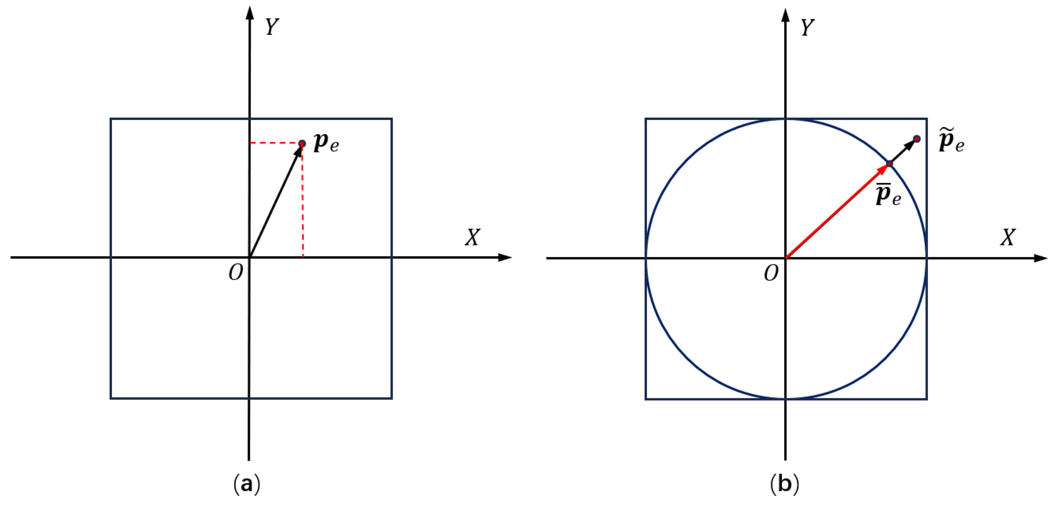
Figure 1. Cartesian representation of the fiber orientation in element e. (a) Original orientation vector p e . (b) Filtered orientation vector p ˜ e and physical orientation vector p ¯ e .
Applsci 15 09242 g001
Figure 2. “Ambiguity” problem of different representations for the fiber orientation. (a) “ 2 π -ambiguity” of the polar representation. (b) Cartesian representation with orientations spanning only 180°.
Applsci 15 09242 g002
Figure 3. Flowchart of CFRCTop for concurrent optimization of the topology and fiber orientations.
Applsci 15 09242 g003
Figure 4. The design domain, displacement, and load boundary conditions for the optimization of a symmetric MBB beam.
Applsci 15 09242 g004
Figure 5. The design domain with 12 elements.
Applsci 15 09242 g005
Figure 6. Optimized design for the MBB problem. (a) Topology and fiber orientations. (b) Collinearity of fiber orientations with the dominant principal stress directions.
Applsci 15 09242 g006
Figure 7. Iteration history of the compliance and volume fraction for the MBB problem.
Applsci 15 09242 g007
Figure 8. Optimized design for the MBB problem obtained by sequentially optimizing of the topology and fiber orientations. (a) Topology and fiber orientations. (b) Collinearity of fiber orientations with the dominant principal stress directions.
Applsci 15 09242 g008
Figure 9. Iteration history of the compliance and volume fraction for the MBB problem obtained by sequentially optimizing the topology and fiber orientations.
Applsci 15 09242 g009
Figure 10. Optimized design obtained from different initialization of the fiber orientations. (a,c,e) The optimized designs for X, Y and random initializations, respectively. (b,d,f) Collinearity of optimized fiber orientations with the dominant principal stress directions for X, Y and random initializations, respectively.
Applsci 15 09242 g010
Figure 11. Iteration history of the compliance for three different initializations of the fiber orientations.
Applsci 15 09242 g011
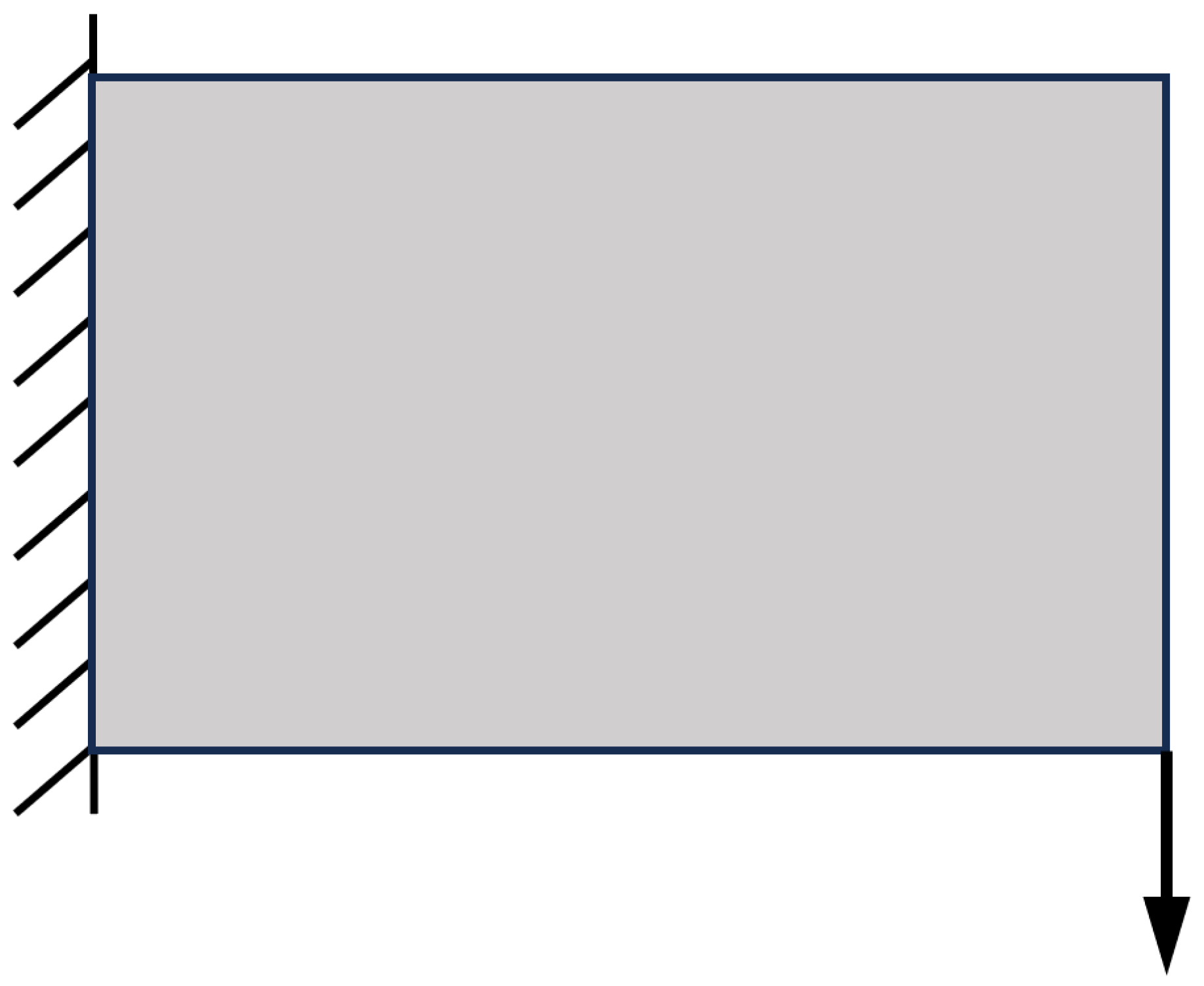
Figure 12. The design domain, displacement, and load boundary conditions for the optimization of a short Cantilever problem.
Applsci 15 09242 g012
Figure 13. Optimized design for the short cantilever problem. (a) Topology and fiber orientations. (b) Collinearity of fiber orientations with the dominant principal stress directions.
Applsci 15 09242 g013
Figure 14. Iteration history of the compliance and volume fraction for the short cantilever problem.
Applsci 15 09242 g014
Figure 15. The design domain, displacement, and load boundary conditions for the optimization of a cantilever problem with two load cases.
Applsci 15 09242 g015
Figure 16. Optimized design for the cantilever problem with two load cases: (a) Topology and fiber orientations. (b) Collinearity of fiber orientations with the dominant principal stress directions under the first load case. (c) Collinearity of fiber orientations with the dominant principal stress directions under the second load case.
Applsci 15 09242 g016
Figure 17. Optimized design for the cantilever problem with two load cases. For the second load case, the load direction is modified to be horizontal. (a) Topology and fiber orientations. (b) Collinearity of fiber orientations with the dominant principal stress directions under the first load case. (c) Collinearity of fiber orientations with the dominant principal stress directions under the second load case.
Applsci 15 09242 g017
Figure 18. Optimized design for the cantilever problem with two load cases. For both load cases, the load directions are modified to be horizontal. (a) Topology and fiber orientations. (b) Collinearity of fiber orientations with the dominant principal stress directions under the first load case. (c) Collinearity of fiber orientations with the dominant principal stress directions under the second load case.
Applsci 15 09242 g018
Figure 19. The design domain, displacement, and load boundary conditions for the optimization of a short Cantilever problem with a passive region.
Applsci 15 09242 g019
Figure 20. Optimized design for the short cantilever problem with a passive region. (a) Topology and fiber orientations. (b) Collinearity of fiber orientations with the dominant principal stress directions.
Applsci 15 09242 g020
Figure 21. Average computation time per iteration for the MBB problem with different resolutions and filter radii.
Applsci 15 09242 g021
Figure 22. Average computation time per iteration obtained with the updated version of the codes for the MBB problem with different resolutions and filter radii.
Applsci 15 09242 g022
Table 1. Comparison of numerical performance between the Top and CFRCTop codes for the MBB problem with rmin = rmin_p = 3.0. t F , t A , t S , t S A , t U are the average computation times for filtering, assembly, equilibrium equation solve, sensitivity analysis, and design update, respectively.
Ω h 300 × 100 600 × 200 900 × 300 1200 × 400
TopCFRCTopTopCFRCTopTopCFRCTopTopCFRCTop
t F 0.00080.00230.00300.00870.00790.02600.01300.0412
t A 0.03630.06630.20980.30460.50560.71230.85281.2492
t S 0.15390.13190.70810.56011.82771.68323.46852.5831
t S A 0.00410.01360.01300.04260.03290.10020.05030.1559
t U 0.04410.04860.16640.19380.66310.69780.95141.0766
The time values in the table are in seconds.
Table 2. Comparison of numerical performance between the Top and CFRCTop codes for the MBB problem with rmin = rmin_p = nelx/100. t F , t A , t S , t S A , t U are the average computation times for filtering, assembly, equilibrium equation solve, sensitivity analysis, and design update, respectively.
Ω h 300 × 100 600 × 200 900 × 300 1200 × 400
TopCFRCTopTopCFRCTopTopCFRCTopTopCFRCTop
t F 0.00080.00230.01200.03280.05370.16310.15990.4570
t A 0.03630.06630.23040.32160.49630.71460.87771.2334
t S 0.15390.13190.72620.58031.82491.70113.51272.6115
t S A 0.00410.01360.03240.06260.12510.19690.34310.4488
t U 0.04410.04860.64120.67573.30953.75389.70329.9716
The time values in the table are in seconds.
Table 3. Comparison of numerical performance between the TopU and CFRCTopU codes for the MBB problem with rmin = rmin_p = 3.0. t F , t A , t S , t S A , t U are the average computation time for filtering, assembly, equilibrium equation solve, sensitivity analysis, and design update, respectively.
Ω h 300 × 100 600 × 200 900 × 300 1200 × 400
TopUCFRCTopUTopUCFRCTopUTopUCFRCTopUTopUCFRCTopU
t F 0.00040.00110.00070.00200.00150.00730.00230.0105
t A 0.03830.06840.21320.30310.49110.70980.86311.2767
t S 0.16250.13990.71630.55981.84121.70143.45782.6024
t S A 0.00340.01290.00910.03830.02070.09060.03200.1422
t U 0.02340.02580.04630.06010.27850.32170.40650.4593
The time values in the table are in seconds.
Table 4. Comparison of numerical performance between the Top and CFRCTop codes for the MBB problem with rmin = rmin_p = nelx/100. t F , t A , t S , t S A , t U are the average computation times for filtering, assembly, equilibrium equation solve, sensitivity analysis, and design update, respectively.
Ω h 300 × 100 600 × 200 900 × 300 1200 × 400
TopUCFRCTopUTopUCFRCTopUTopUCFRCTopUTopUCFRCTopU
t F 0.00040.00110.00180.00430.00580.01670.01390.0357
t A 0.03830.06840.23620.32540.48370.71500.86891.2606
t S 0.16250.13990.73030.57581.79401.69663.51742.6221
t S A 0.00340.01290.01170.04260.02690.09400.05190.1562
t U 0.02340.02580.10830.12190.50110.53141.03571.0914
The time values in the table are in seconds.
Disclaimer/Publisher’s Note: The statements, opinions and data contained in all publications are solely those of the individual author(s) and contributor(s) and not of MDPI and/or the editor(s). MDPI and/or the editor(s) disclaim responsibility for any injury to people or property resulting from any ideas, methods, instructions or products referred to in the content.