Article

Stackade Ensemble Learning for Resilient Forecasting Against Missing Values, Adversarial Attacks, and Concept Drift

by
Mohd Hafizuddin Bin Kamilin
1,* and
Shingo Yamaguchi
2,*
1
Department of Intelligent System Engineering, National Institute of Technology, Ube College, Yamaguchi 755-8555, Japan
2
Graduate School of Sciences and Technology for Innovation, Yamaguchi University, Yamaguchi 753-8511, Japan
*
Authors to whom correspondence should be addressed.
Appl. Sci. 2025, 15(16), 8859; https://doi.org/10.3390/app15168859
Submission received: 16 July 2025 / Revised: 7 August 2025 / Accepted: 9 August 2025 / Published: 11 August 2025

Abstract

Featured Application

Stackade Ensemble Learning could make the smart grid better at predicting electricity usage by combining several solutions to reduce error accumulation and improve accuracy, even when there are missing values, adversarial attacks, and concept drift.

Abstract

Machine learning is often implemented in smart grids to help with electricity load forecasts, which are challenging to process or compute using conventional approaches. However, most of the proposed techniques were created with the assumption that the data was clean with a consistent distribution. However, this is not always the case because there can be missing data due to distributed denial-of-service attacks, changes in data patterns that make predictions less accurate, and small perturbations from adversarial attacks that trick the machine learning into making wrong forecasts. While several approaches have been suggested, they are limited to a trivial solution, and the sequential operation needed to correct the input will accumulate errors from inadequate correction. This research proposes a novel approach called Stackade Ensemble Learning. It works by cascading the dependent input corrections with enhanced forecasting models to reduce the error accumulation. Then, the outputs were stacked to combine the results and improve the forecast. The results show 348.4002% of mean absolute error score improvement against the federated solution and 30.3783% against the trivial solution on compounded problem, proving its effectiveness.

1. Introduction

The advancement of digital infrastructure helps bring the digital transformation to the energy sector in the form of smart grids. Smart grids help manage the dynamic pricing based on supply and demand [1], balance the load across the networks [2], and smooth the integration of renewable energy with the grid [3] using machine learning (ML) to address the changes proactively. These benefits enable the provision of affordable, reliable, and clean energy, a feat that would be challenging to achieve using only a conventional statistical model, which struggles to process short-term loads that exhibit complex patterns [4]. These examples show the benefits of ML implementation in smart grids. However, most of the proposed MLs were made with the assumption that the input would be clean to avoid negatively impacting the forecasting accuracy [5].
Because these conditions are not guaranteed in real-world applications, forecasting accuracy often degrades due to the deviation shown in the following:
  • Missing values (MV);
  • Adversarial attacks (AA);
  • Concept drift (CD).
Although AA are only attributed to the data compromised by the hackers, there are plenty of reasons that could cause MV and CD. In this paper, distributed denial-of-service (DDoS) is attributed to the high percentage of MV, while the seasonal change caused the CD. Figure 1 summarizes the causes for the deviation found in the data.
MV caused by DDoS floods the smart grid network, which causes data packets to become lost between the sensors and the servers [6]. Without imputation to substitute the MV or hardening the forecasting model, the accuracy of electricity load forecasts will worsen as the percentage of MV increases [7]. As noted by Cloudflare, DDoS attacks in 2024 have increased compared to the prior year [8], necessitating better imputation.
Besides DDoS, smart grids are also at risk from AA. The IBM X-Force 2025 Threat Intelligence Index [9] shows that cybercriminals will be more incentivized to target artificial intelligence (AI) technologies as the market share increases to 50%. Although it is not yet observed in real life, they could fool ML by inserting crafted noises into the input [10]. Solutions usually depend on detection, model hardening, and data correction [11].
Finally, CD explains the situation when the current data distribution diverges from data used to train, invalidating the forecasting model and reducing the accuracy [12]. When the input exhibits new patterns or when the values exceed the scale used during training due to the seasonal changes, the forecasting model will struggle to make accurate predictions without retraining or using feature scaling designed to handle outliers [13].
To investigate the patterns and trends in enhancing the forecasting accuracy in smart grids against MV, AA, and CD, bibliometric analysis was performed. From 1 January 2015 to 31 July 2025, the top 50 most relevant references were gathered for each year using the specific keyword combinations that are shown below:
  • “Forecast” “Smart Grid” “Missing Values”—“Adversarial Attacks”—“Concept Drift”;
  • “Forecast” “Smart Grid” “Adversarial Attacks”—“Concept Drift”—“Missing Values”;
  • “Forecast” “Smart Grid” “Concept Drift”—“Missing Values”—“Adversarial Attacks”;
  • “Forecast” “Smart Grid” “Concept Drift” “Missing Values” “Adversarial Attacks”.
Then, the duplicated references found in Google Scholar and ScienceDirect were removed before the remaining 1799 references were processed with VOSviewer 1.6.20 [14] to extract the keywords from the title and abstract. Figure 2 and Figure 3 are obtained by using binary counting with the minimum number of occurrences set to 50 and displaying only 60% of the most relevant keywords.
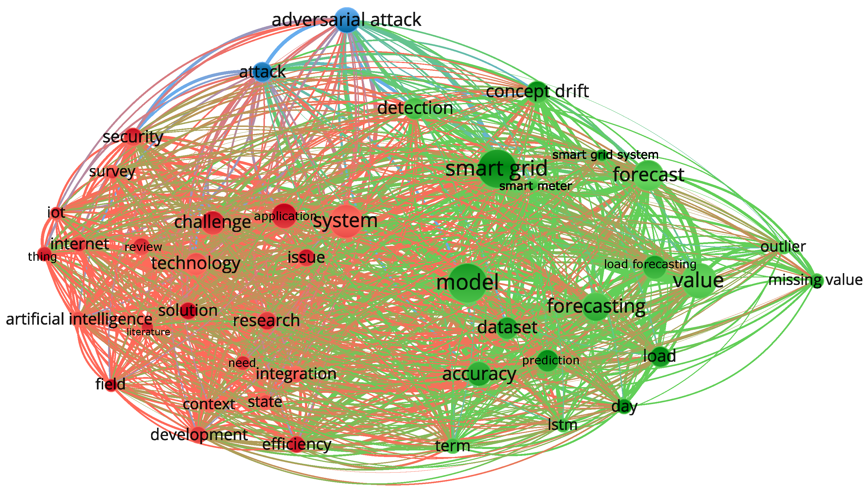
In Figure 2, the bibliographic analysis identifies three clusters. The green cluster shows the core technical focus in smart grid forecasting, such as preprocessing the data against the outlier, MV, and CD to improve the data quality and forecasting accuracy. The red cluster highlights the focus on integrating the Internet of Things (IoT) for data gathering and AI for forecasting in smart grids, in addition to addressing the security and efficiency challenge. Finally, the blue cluster shows adversarial attacks as an emerging topic that is closely related to system security and CD detection.
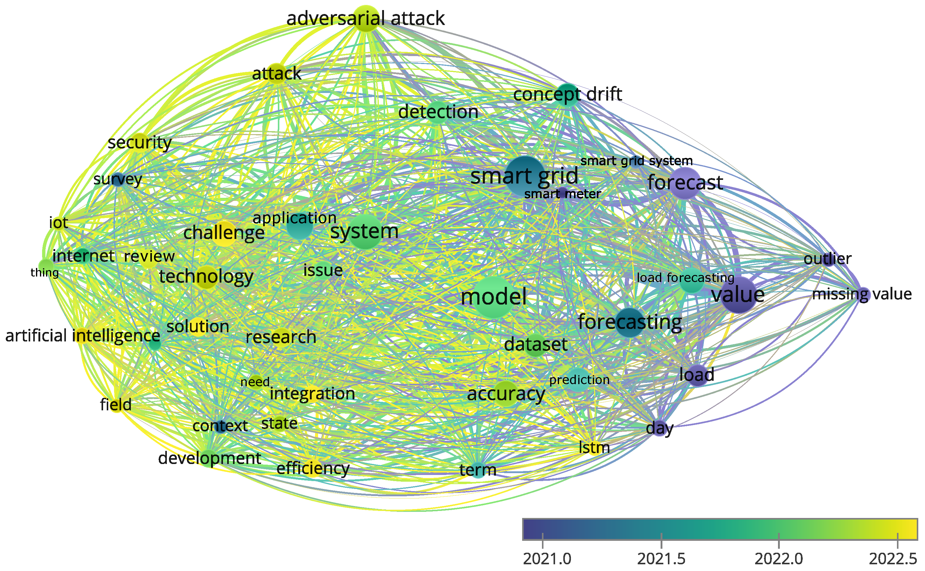
In Figure 3, bibliographic analysis indicates that research trends on MV and CD were significant in earlier years for maintaining data quality and enhancing basic forecasting accuracy. Afterwards, the trend shifted to integrating with smart grid technologies for optimizing the operation. Finally, as the technologies become widely deployed, the trend is moving to protect smart grids against AA, ensuring optimal operation. Although there are substantial references found on MV, AA, and CD, the research done in unifying the solutions is still new.
By plotting the reference count from the data used in the bibliographic analysis, there are only 13 references that have the keywords “missing values,” “adversarial attacks,” and “concept drift,” as shown in Figure 4. Furthermore, after excluding surveys, reviews, and irrelevant references, there is only one study focusing on detecting AA and CD as a form of prevention, followed by data imputation on MV.
According to the research trends shown in Figure 3, MV and CD are commonly associated with low data quality instead of cyberattacks, which is counterintuitive, as the attackers could utilize these issues to enhance AA. Additionally, the inadequate data correction done to resolve MV, AA, and CD could cause the errors to accumulate, making trivial solutions that aim to rectify the issues via cascading operation less effective. These issues could lead to higher electricity prices because of unoptimized operations and grid instability, which disrupt essential services [15,16].
A common tactic to improve ML often relies on using additional data with a strong correlation to the target forecast [17]. These data help improve the imputation accuracy, provide reference data to correct the anomalies, and offer additional information to follow the trends. Figure 5 shows the example that leverages a multivariable forecasting model for improving the electricity load forecast in New York City (NYC), with Dunwoodie and Genesee as the additional data.
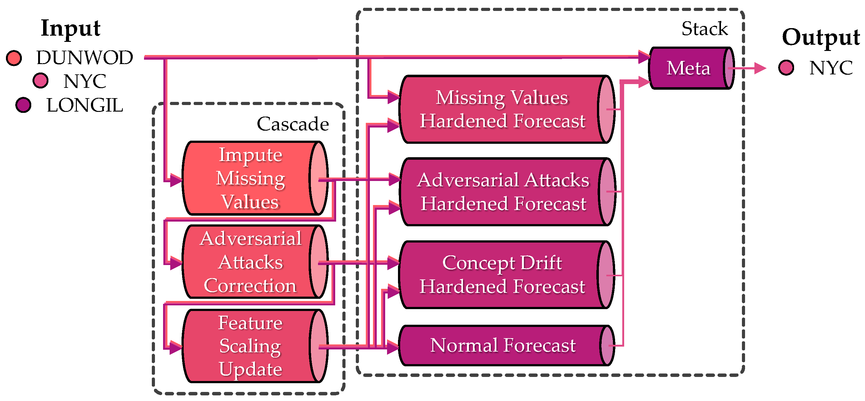
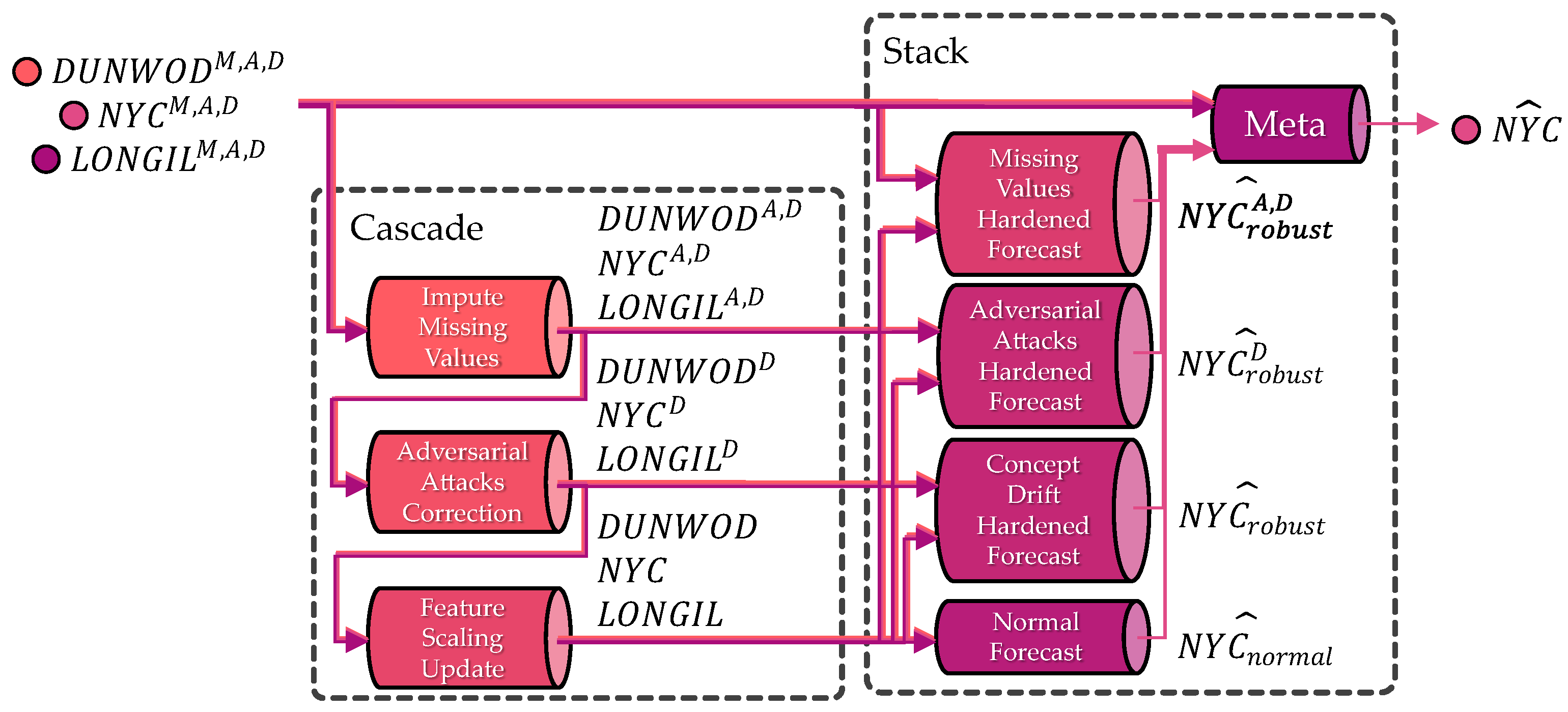
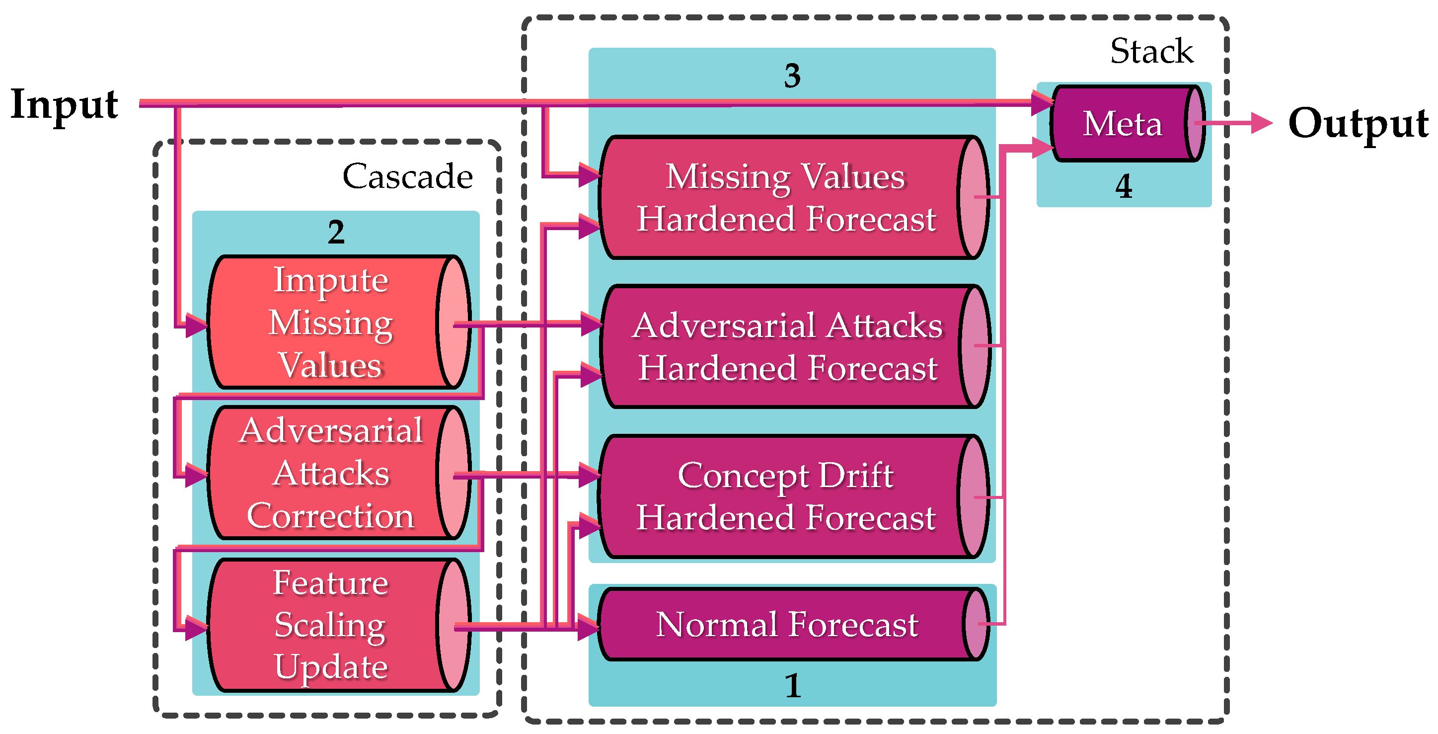
This paper expands upon this tactic by proposing a new ensemble method called Stackade Ensemble Learning (StEL), which is a portmanteau of stack and cascade. As shown in Figure 6, StEL is a multivariable forecasting model that consists of multiple modules. It leverages the strength of Cascading Ensemble Learning (CEL) [18] for input correction on top of Stacking Ensemble Learning (SEL) [19] to unify multiple solutions. While CEL corrects the input based on their priority, the SEL arrangement in StEL compares pre-correction and post-correction data from CEL to account for inadequate corrections and fine-tune the forecast before being aggregated by the metamodel. Section 3 will discuss the concept in detail.
After the introduction in Section 1, Section 2 provides the preliminary information on MV, AA, CD, and the compounding problem. Then, the previous studies done to solve the problems are introduced. Section 3 presents the novelty of the StEL concept to leverage the strength of CEL and SEL, followed by the modules used in it. Then, Section 4 presents the dataset, StEL application, and the baseline methods to compare. Thereafter, Section 5 discusses the results between StEL and baseline methods, followed by a conclusion and future planning in Section 6.

2. Preliminary

2.1. Problems

2.1.1. Missing Values

This paper attributes MV to the packet drop caused by the DDoS. Existing studies indicate that the percentage of packet loss due to the DDoS attacks could exceed 90% [20,21]. Although Cloudflare shows that 89% of DDoS attacks on Layer 3 and Layer 4 are less than 10 min [22], the MV is applied to the entire sequence for benchmarking purposes.
To formalize the problem, the load time series X is defined as X = x 1 , x 2 , x 3 , , x N , with N as the number of loads and missing percentage as p e r c e n t a g e 0 , 0.1 , 0.2 , , 0.9 . With the number of MV as t o t a l = N · p e r c e n t a g e and index set as i n d e x = 1 , 2 , 3 , , N , indices from i n d e x are randomly selected to form a subset c h o s e n i n d e x such that c h o s e n = t o t a l . The time series X m with missing elements is defined in Equations (1) and (2), with the missing element represented as ⌀.
X m = x 1 m , x 2 m , x 3 m , , x N m
x i m = , if i c h o s e n x i , if i c h o s e n
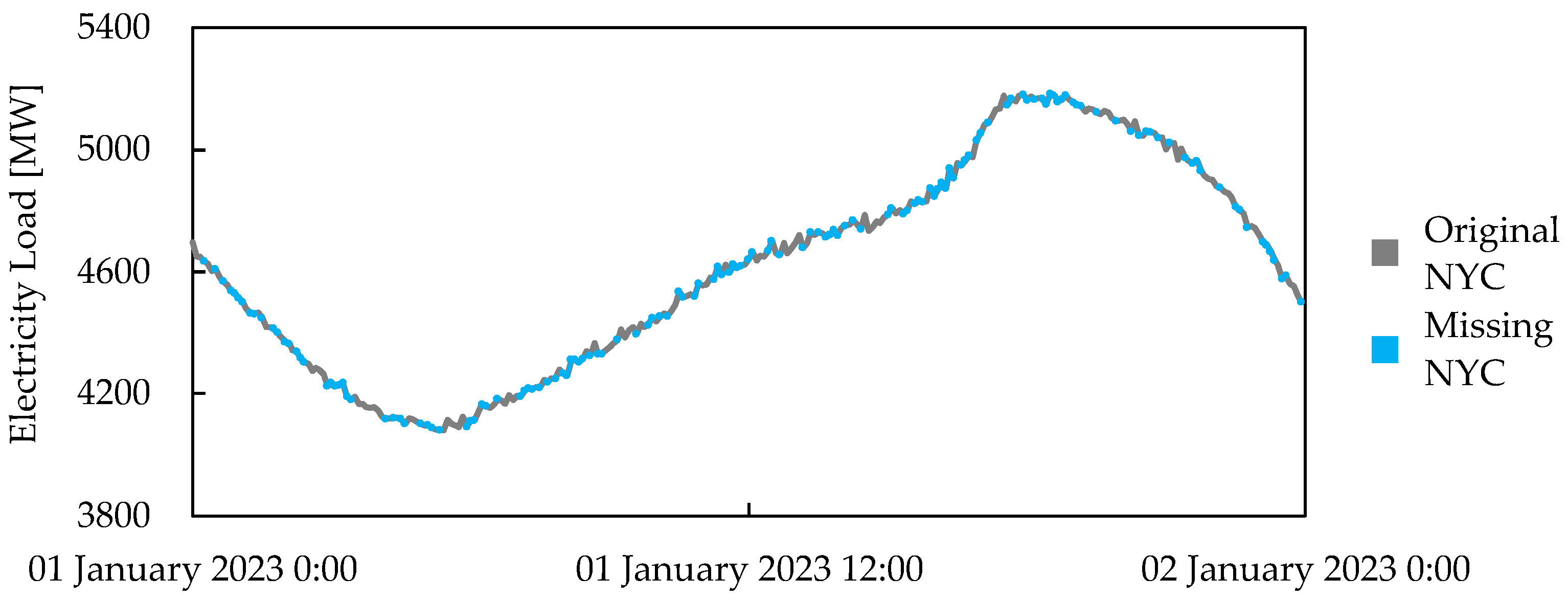
Algorithm 1 shows the MV simulation with seeded randomization for replicability. Once the randomization mechanism was seeded, it created a copy of X and found the number of elements in it. Then, the total number of missing values was calculated, followed by generating the index based on the number of elements in X. Thereafter, random indices were chosen to be inserted with MV. Figure 7 shows the example on NYC load data with 50% of MV inserted. Although this paper measures the forecasting accuracy in 3-month intervals, only the first 24 h of data are shown to make it easier to visualize the difference between the original sequence and the sequence with MV.
Algorithm 1 Missing values with varying percentages implementation
Input: Time series X, missing percentage p e r c e n t a g e , randomization seed s e e d
Output: Time series with missing values X m
  1: Function missing_values ( X ,   p e r c e n t a g e )
  2:     Apply randomization seed: randomization _ seed ( s e e d )
  3:     Copy the sequence: X m copy ( X )
  4:     Find the total element in X: N len ( X )
  5:     Find total number of missing values: t o t a l int ( N · p e r c e n t a g e )
  6:     Generate index: i n d e x 1 , 2 , 3 , , N
  7:     Choose random indices: c h o s e n choose ( i n d e x , t o t a l )
  8:     Replace value with null on chosen indices: X m [ c h o s e n ]
  9:     return  X m
 10: End Function

2.1.2. Adversarial Attacks

In this paper, projected gradient descent (PGD) was used to create the AA on the electricity load dataset. PGD uses iterative adversarial creation with random perturbation initialization to ensure the perturbation ϵ 0 , 0.01 , 0.02 , , 0.09 added is constrained using the projector operator Π X , ϵ [23].
The difference from other commonly used AA, such as the fast gradient sign method (FGSM) and basic iterative method (BIM), is not only that it calculated the gradient and added perturbation iteratively to make the attack more robust, but also that the added random perturbation initialization helped PGD in exploring a wider range of effective adversarial examples to trick ML into making incorrect forecasts [24].
To initialize the random perturbation, a noise vector n o i s e was sampled from the uniform distribution U ( ϵ , ϵ ) . Then, n o i s e was added to X before being constrained within the ϵ -ball centered at X, which is denoted as Π X , ϵ , as shown in Equation (3). Once initialized, the loss between the forecast on the original data and the perturbed data was calculated L X ^ , X ^ A , ( j ) to obtain the gradient X . The  sign ( ) function is then applied to return the sign of each component of the gradient vector to get either −1, 0, or 1 to determine the direction to add the perturbation. Finally, α determines the strength to move the signs before constraining it with Π X , ϵ . This operation was repeated by adding the new perturbation on the previously perturbed X A , ( j ) based on the number of iterations i t e r a t i o n , as shown in Equation (4).
X A , ( 0 ) = Π X , ϵ X + n o i s e , where n o i s e U ( ϵ , ϵ )
X A , ( j + 1 ) = Π X , ϵ X A , ( j ) + α · sign X L X ^ , X ^ A , ( j ) , where 1 j i t e r a t i o n
Figure 8 is the stacked long short-term memory (LSTM) [25] model used in this example. It utilizes one hour of electricity load ( 0 t < 12 ) to forecast the next one hour ( 12 t < 24 ) . The layers consist of 48 and 24 units, using hyperbolic tangent (TanH) as the activation function and sigmoid for the recurrent activation. Adam with a learning rate of 0.0001 was used to train, with an early stop function to stop the training if the mean squared error (MSE) score improvement is less than 0.001 for three consecutive times.
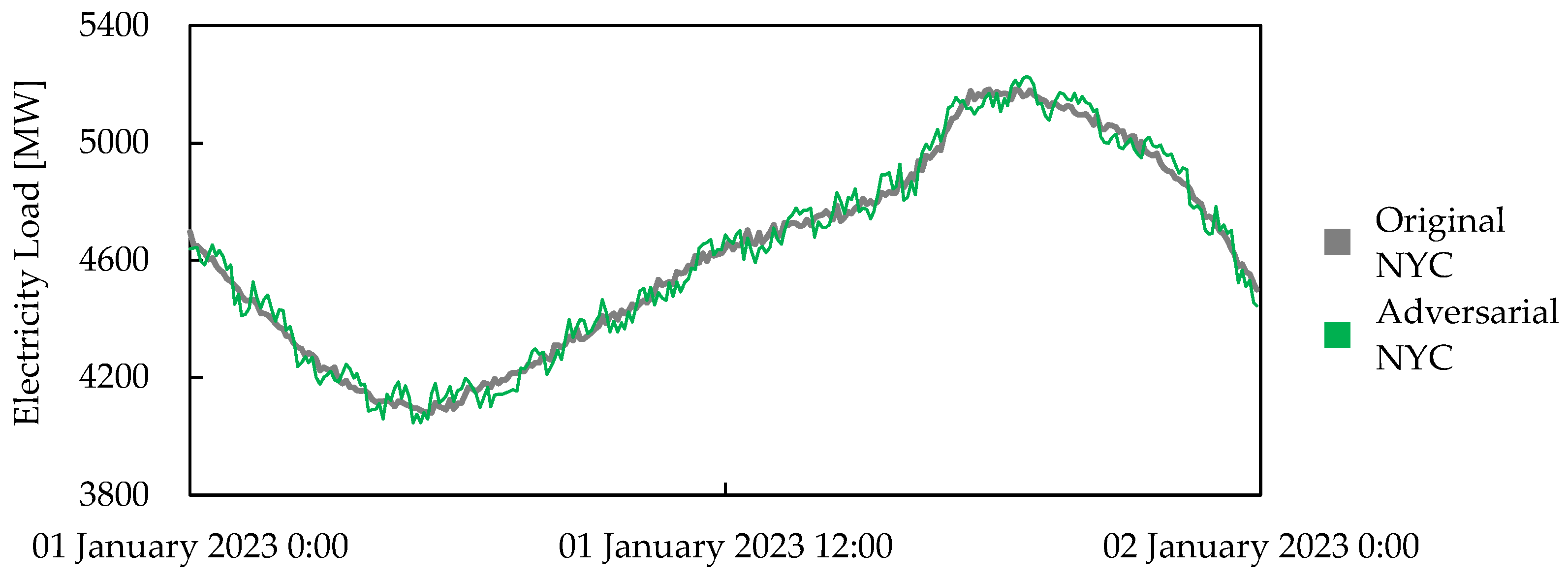
Once the LSTM model was trained on NYC’s electricity load from 1 January 2023 to 12 December 2023, it was used as a surrogate model in Algorithm 2 to generate the PGD-based perturbation on X, followed by a PGD example of ϵ = 0.01 and i t e r a t i o n = 10 in Figure 9. To reduce the number of parameters needed, α = ϵ / i t e r a t i o n .
Algorithm 2 Projected gradient descent implementation
Input: Time series X, surrogate model surrogate , intensity ϵ , iteration i t e r a t i o n
Output: Adversarial time series X A
  1:   Function pgd_sample ( X ) , surrogate , ϵ , i t e r a t i o n )
  2:    Get forecast using surrogate model: X ^ surrogate ( X )
  3:    Create a copy of the array: X A copy ( X )
  4:    Generate uniform noise: n o i s e random.uniform( ϵ , ϵ , len(X))
  5:    Add noise to the copied array: X A X A + n o i s e
  6:    Get minimum clipping: m i n i m u m X ϵ
  7:    Get maximum clipping: m a x i m u m X + ϵ
  8:    Clip the added noise: X A clip( X A , m i n i m u m , m a x i m u m )
  9:    Calculate the alpha: α ϵ / i t e r a t i o n
10:       for  j = 0 to i t e r a t i o n 1  do
11:        with GradientTape() as tape do
12:           Tape on X A : tape.watch( X A )
13:           Get prediction: X A ^ surrogate ( X A )
14:           Compute loss: l o s s mean _ squared _ error ( X ^ , X A ^ )
15:        end with
16:        Compute gradient: g r a d i e n t tape . gradient ( l o s s , X A )
17:        Insert perturbation: X A X A + α · sign ( g r a d i e n t )
18:        Clip perturbations: X A clip( X A , m i n i m u m , m a x i m u m )
19:    end for
20:    return  X A
21: End Function

2.1.3. Concept Drift

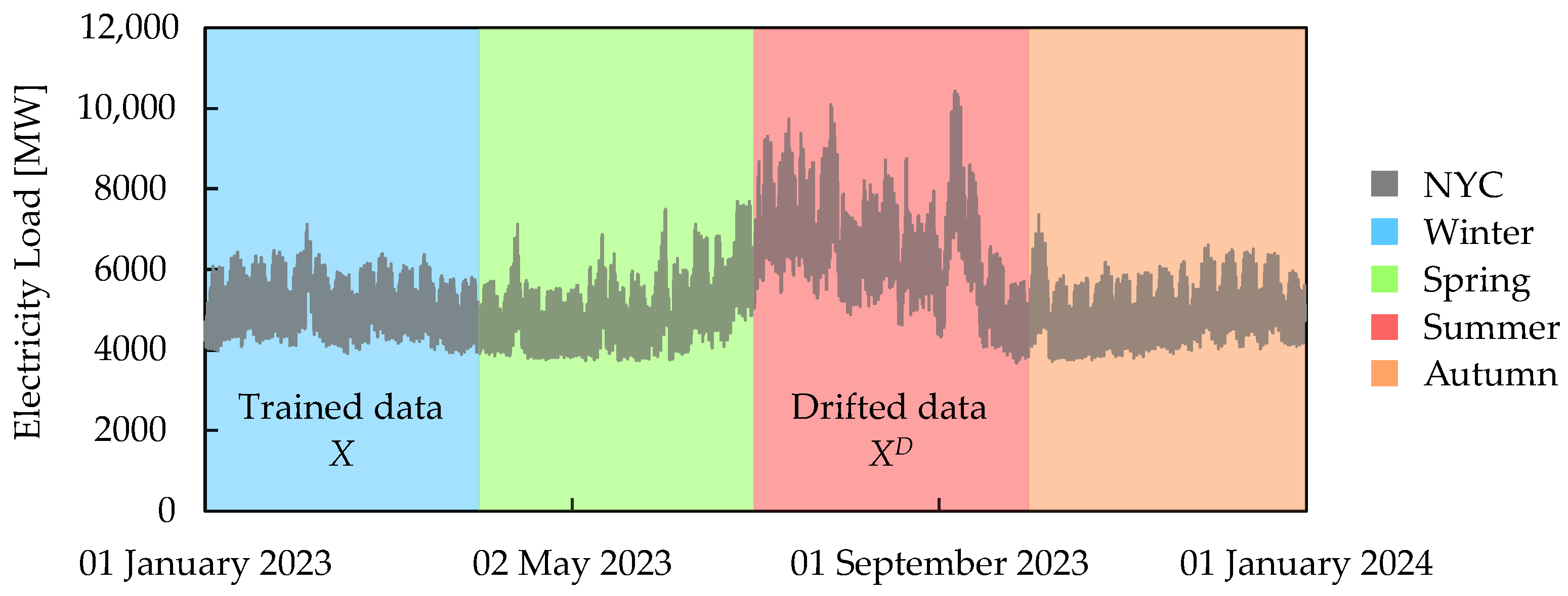
While there are many reasons that cause CD [26], such as changing user preferences, aging sensors, or external factors that are uncountable, this paper focuses on seasonality changes that affect the electricity consumption. Figure 10 shows that electricity load during the summer, which is denoted as X D to indicate it is a drifted sequence, is higher than X in the winter. Although this observation seems counterintuitive, the low electricity consumption in winter is primarily because fossil fuel-based heating is commonly used in New York State due to its cost and efficiency [27].
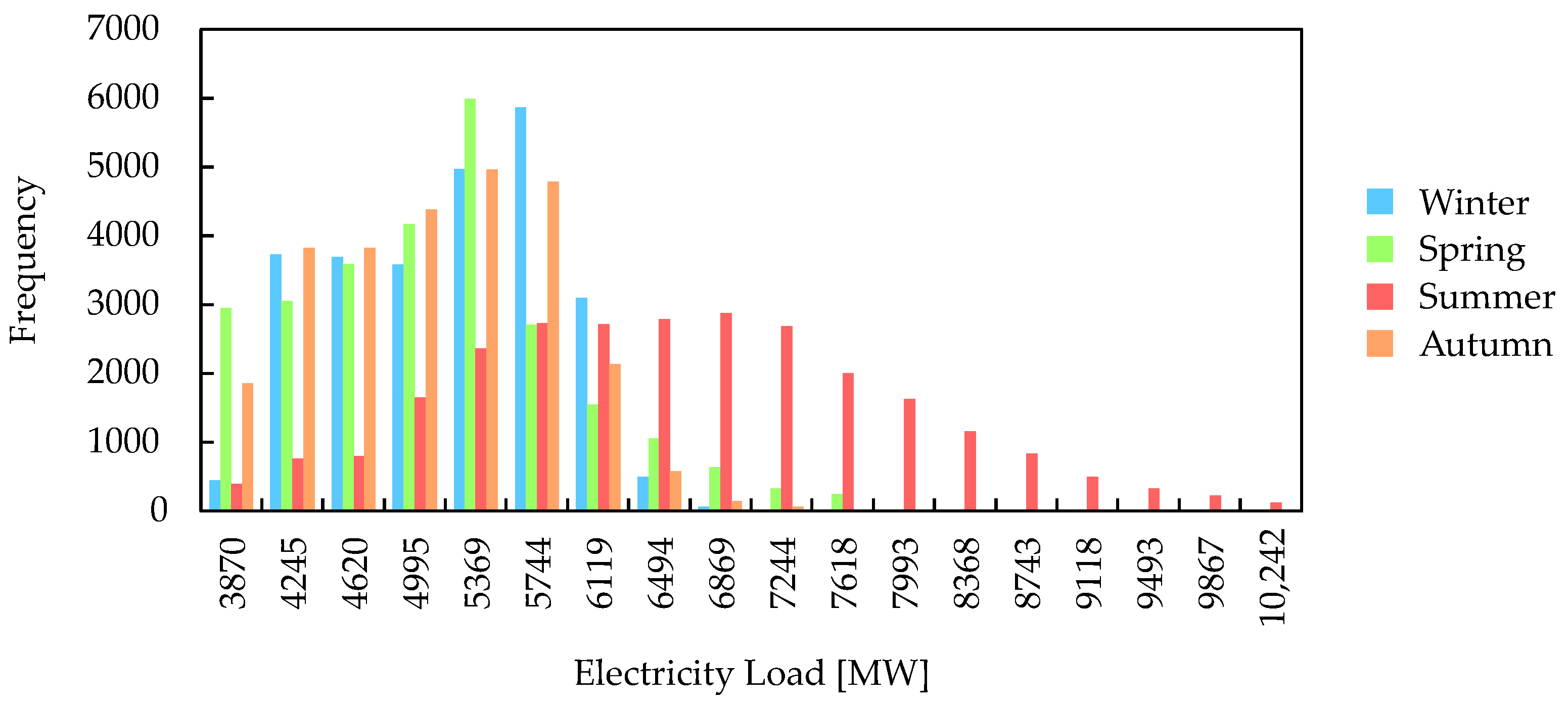
Figure 11 reaffirmed that X D is a drifted sequence due to the distribution deviation found using the NumPy 2.1.3’s histogram function [28,29]. If there is no countermeasure taken against the forecaster trained with X, the accuracy could degrade.

2.1.4. Compounding Problem

In addition to the MV, AA, and CD, the forecasting model also faces the compounding problem where multiple issues happen at the same time. This pitfall could negatively affect the previously proposed solutions that focus on resolving only one issue with no consideration for other problems or trivial solutions that rely solely on cascading multiple solutions. By defining functions to represent AA as f A ( X ) = X A and a function for MV as f M ( X ) = X M , the issue that arose in a sequence with seasonal drift X D is defined in Equation (5).
X M , A , D = f M ( f A ( X D ) )
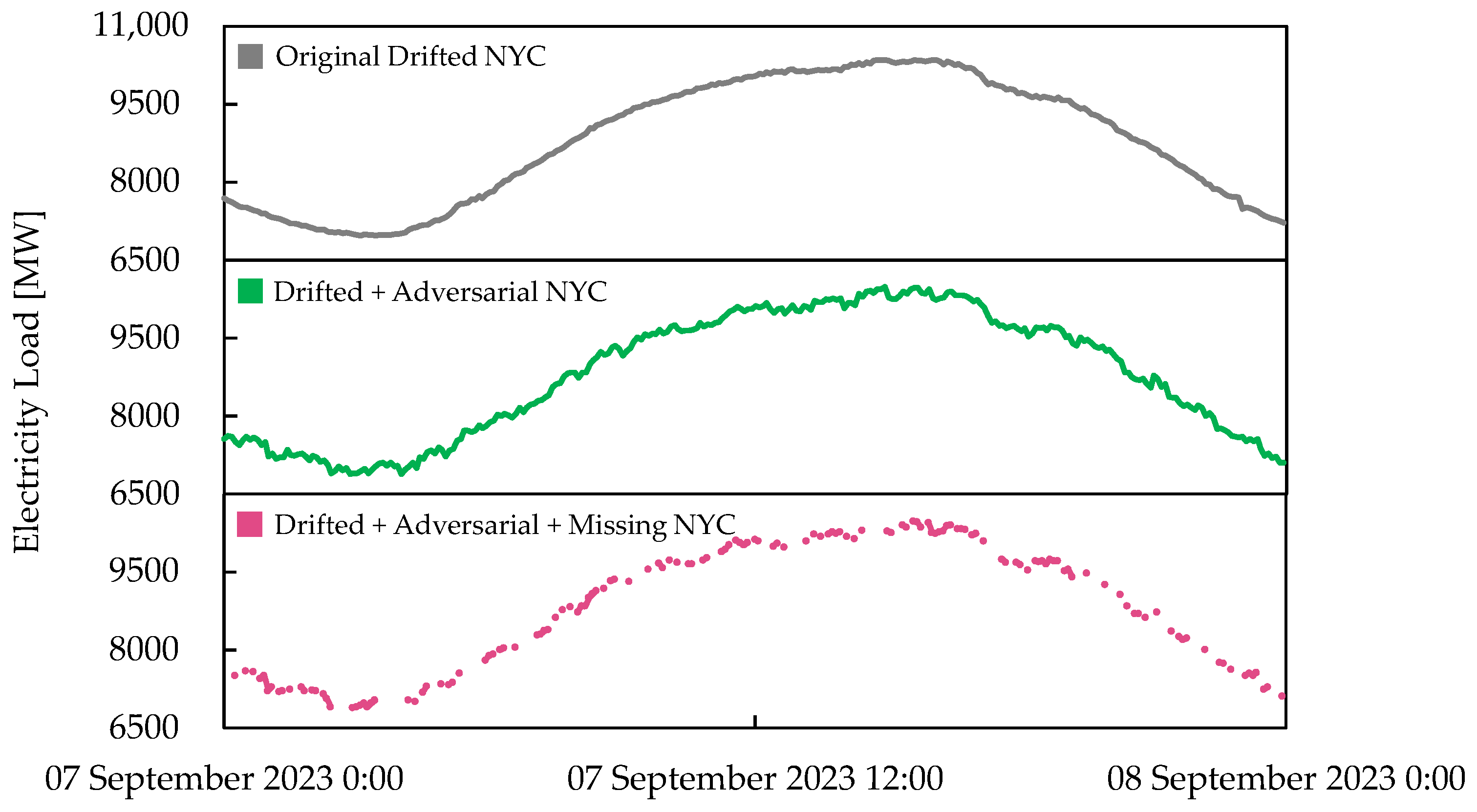
The compounding problem illustrates how an attacker might add AA to data with seasonal drift, which could further reduce accuracy, and then use MV from DDoS attacks to conceal the changes. Even though the MV could potentially eliminate the disturbance meant to trick the forecaster, the perturbation shifted the remaining values, which lowered the imputation accuracy. Figure 12 demonstrates how the compounding problem with 50% of MV and ϵ = 0.02 changed the original drifted data in NYC. Although the ϵ values were increased to 0.02, the perturbation is less noticeable than in Figure 9. This difference arises from a fixed amount of perturbation added by Algorithm 2, which is constrained within the ϵ -ball centered at X. Because the electricity load data in summer has a larger magnitude compared to winter data, the perturbation has a lesser statistical and visual impact when applied to the summer subset.
To properly address the compounding problem, the forecasting model must be able to individually address the issues found in the input data. However, the inaccuracies in handling each of the issues could carry on to the next solutions, causing error accumulation.

2.2. Previous Studies

Existing studies for solving either MV, AA, CD, or the combination of them are classified into the following categories:
  • Single-purpose solution;
  • Multi-purpose solution.
This subsection discusses the differences between single-purpose and multi-purpose solutions, in addition to the limitation that this paper aims to resolve.

2.2.1. Single-Purpose Solution

For handling MV, Hou et al. [30] proposed a hybrid imputation method that combines Random Forest, Spearman-weighted K-Nearest Neighbors, and a Levenberg–Marquardt backpropagation neural network to process seasonality and weather for improving the imputation of electricity load data. Hwang et al. [31] proposed to cluster similar data points before applying a generative adversarial network (GAN) for the specified cluster to further improve the accuracy. Although the proposed single-purpose solutions provide high imputation accuracy, they cannot handle the perturbation inserted by AA and CD due to the seasonal change.
While AA detection shares the same concept as hardware anomaly detection [32], model hardening and data correction are more favored due to real-time operation in smart grids. To address AA, Yihong Zhou et al. [33] suggested a deep learning (DL) model that uses Bayesian neural networks to add randomness to the model’s predictions, making it more robust. Mahmoudnezhad et al. [34] designed a DL model that uses stacked multilayer denoising autoencoders to correct the anomalies found in the input before forecasting it with a GAN that was hardened with adversarial training. As these are single-purpose solutions, the MV in electricity load data must be imputed first. Additionally, it does not address the issue with CD.
Solving CD requires the forecasting model to continuously learn to catch up with the latest trends. Azeem et al. [35] created a dynamic attention-based LSTM in ensemble configuration to adapt to CD via continuous update, in addition to updating the features’ importance as the trends change to improve accuracy. Jagait et al. [36] proposed online ensemble learning that combines an adaptive recurrent neural network with a rolling autoregressive integrated moving average to improve accuracy with continuous updates. However, the solutions cannot address MV and AA without relying on imputing the MV and data correction or model hardening against the AA.

2.2.2. Multi-Purpose Solution

As the previous studies mainly focused on solving specific issues encountered when forecasting in smart grids, it limits their applicability beyond the scope they are designed for. Referring back to Figure 4, out of 13 references found that match the keywords, there is only one relevant research paper that fits in the context.
Yang Zhou et al. [37] created a blockchain federated learning framework for digital twin modeling in smart grids. It solve MV via interpolation, lowering the contribution of local models compromised with AA via a reputation-based scoring system, and automatically updating models by monitoring the changes in the conformal score. Table 1 summarizes the differences, highlighting the lack of studies on multi-purpose solutions.
While the multi-purpose solution tackles the mentioned issues, it does not consider the negative effect from inaccurate MV imputation [38]. Additionally, excluding the local models or data compromised with AA is not feasible in a situation where both are necessary to obtain a specific forecast. Additionally, it may experience poor accuracy due to data heterogeneity [39], which necessitates the global model to be retrained again on the local data. Finally, the solutions to address AA and CD only provide protection during the training phase. Section 3 discusses how StEL resolves these problems, in addition to mitigating the issue with stacking errors when combining multiple solutions.

3. Implementation

3.1. Stackade Ensemble Learning

StEL is designed to leverage the CEL’s capability to sequentially correct the anomalies found in the input data and SEL’s strength to combine multiple forecasts into one. The approach of sequentially correcting the data allows StEL to utilize the required data with no omissions, and combining multiple forecasts helps StEL be more robust without relying on federated learning.
Combining CEL and SEL might solve the issues with blockchain federated learning mentioned by Yang Zhou et al. [37], but it is not as simple as just connecting the last correction from CEL to SEL, because any errors from earlier corrections will carry over. Additionally, input data must be processed based on its priority and compatibility with other data corrections. This subsection discusses the StEL implementation and the approach taken to resolve the mentioned issues.

3.1.1. Ensemble Strategy

The compatibilities between the solutions influence how they are connected in StEL, which restricts the order of operations to fix the data and how it is used to make an accurate forecast. StEL classifies the solutions as data correction and hardened forecasters. While solutions that focus on data correction are used in the cascading setup, hardened forecaster solutions and the normal forecaster are used in the stacking setup instead. This grouping allows StEL to utilize the strength of CEL and SEL at the same time.
In the cascading operation, the solutions for correcting the data are done in the order of imputing the MV, correcting the AA, and adapting the feature scaling to CD. The reason imputation is done first is not only to preserve data integrity but also because the subsequent operations assume complete data to work on [40]. After the imputation, a data correction is done to address the perturbations that affect the next operation. Imputing the missing values is a prerequisite for helping the solution accurately identify and resolve the AA [41]. Updating the feature scaling to address CD is done last because most CD detection methods expect the data to be clean before assessing changes in distribution and model accuracy [42]. Table 2 summarizes the solution’s priority and dependencies.
In the stacking operation, the base models are run in parallel to forecast the electricity loads on the designated zone before they are combined by the metamodel. Although the stacking operation does not require a specified order for processing base models, the base models receive a different subset of data to forecast, which diverges from a standard SEL implementation. Figure 13 shows the hardened forecasters received pre-correction and post-correction data for the problems they are designed for, with the exception of the normal forecaster. This configuration helps the hardened forecasters to identify any inadequacy from the correction and adjust the forecast based on how far it diverges. The same concept is also utilized by the metamodel to adjust and aggregate the forecasts.
The modules in the cascading operation are defined as C o r r e c t M , C o r r e c t A , and  C o r r e c t D to correct MV, AA, and CD. By redefining the N Y C M , A , D , D U N W O D M , A , D , and  W E S T M , A , D as X M , A , D , Y M , A , D , and  Z M , A , D , Equations (6)–(8) show the cascading operation to sequentially correct the input.
X A , D , Y A , D , Z A , D = C o r r e c t M ( X M , A , D , Y M , A , D , Z M , A , D )
X D , Y D , Z D = C o r r e c t A ( X A , D , Y A , D , Z A , D )
X , Y , Z = C o r r e c t D ( X D , Y D , Z D )
The modules in the stacking operation are defined as F o r e c a s t M , F o r e c a s t A , and  F o r e c a s t D that are hardened against MV, AA, and CD, followed by F o r e c a s t N o r m a l to be the reference forecast and M e t a to aggregate the forecasts. Equations (9)–(11) take the pre-correction data and post-correction data to forecast, while Equation (12) only forecasts with post-correction data. Finally, the forecast outcomes are aggregated in Equation (13).
X r o b u s t A , D ^ = F o r e c a s t M ( X M , A , D , Y M , A , D , Z M , A , D , X A , D , Y A , D , Z A , D )
X r o b u s t D ^ = F o r e c a s t A ( X A , D , Y A , D , Z A , D , X D , Y D , Z D )
X r o b u s t ^ = F o r e c a s t D ( X D , Y D , Z D , X , Y , Z )
X n o r m a l ^ = F o r e c a s t N o r m a l ( X , Y , Z )
X ^ = M e t a ( X M , A , D , Y M , A , D , Z M , A , D , X r o b u s t A , D ^ , X r o b u s t D ^ , X r o b u s t ^ , X n o r m a l ^ )
Since the solutions inside the cascading and stacking operation correlate with each other, the ensemble arrangement can be adjusted based on the type of anomalies found in the input. For example, when the input only has MV, the  C o r r e c t A and C o r r e c t D , in conjunction with F o r e c a s t A and F o r e c a s t D , are disabled with the output from C o r r e c t M being parsed to F o r e c a s t M and F o r e c a s t N o r m a l before being aggregated with M e t a . This mechanism allows StEL to adapt based on the anomalies detected and reduce unnecessary computation.
This novel strategy of StEL to utilize the strength of CEL and SEL helps to address the error from accumulating due to inadequate data correction methods. Additionally, it allows no exclusion of compromised data that might still be useful to improve the forecast.

3.1.2. Training Strategy

To prepare StEL for handling MV, AA, and CD, the modules are trained in the order shown in Figure 14, where the normal forecaster is trained first, followed by the cascading operation’s modules, the stacking operation’s hardened forecaster, and the metamodel.
This is because the solutions must be able to consider the correction and forecasting inadequacies. Hence, the reason why the missing, adversarial, and drift-hardened forecaster modules need the results from the cascading operation to learn how to improve the forecast based on the inadequate corrections. Similarly, the meta module is trained last because it needs the output from the forecaster modules to learn how to adjust the forecast based on anomalies in the input.
Table 3 and Table 4 show the training data. While normal data represent the original, CD data represent data preprocessed with different scalings, followed by MV and AA processed with the generators in Section 2.1.1 and Section 2.1.2.

3.2. Implemented Solutions

The solutions inside the StEL are implemented based on existing research to tackle the issues with MV, AA, and CD via correction or hardening the forecast. This subsection discusses the solutions implemented in cascading and stacking operations with a focus on improving forecast reliability.

3.2.1. Cascade Modules

The imputation module borrows the commonly used concept to prepare ML for imputations [43]. The concept involves conducting data analysis to identify data points with strong correlations, which enhances the accuracy of imputation. Then, the data targeted for forecast and the data with strong correlation are used to generate the training data with MV using Algorithm 1, where the p e r c e n t a g e { 0 , 0.1 , 0.2 , , 0.9 } and the MV is masked with 1 . The generated data are used to train MLs to impute the MV in the data targeted for forecast and the data with strong correlation.
Similarly, the adversarial correction module uses the data targeted for forecast and the data with strong correlation to generate the training data with AA using Algorithm 2, where the ϵ { 0 , 0.01 , 0.02 , , 0.09 } . The generated data are then used to train the MLs to reconstruct the data without the perturbation [11].
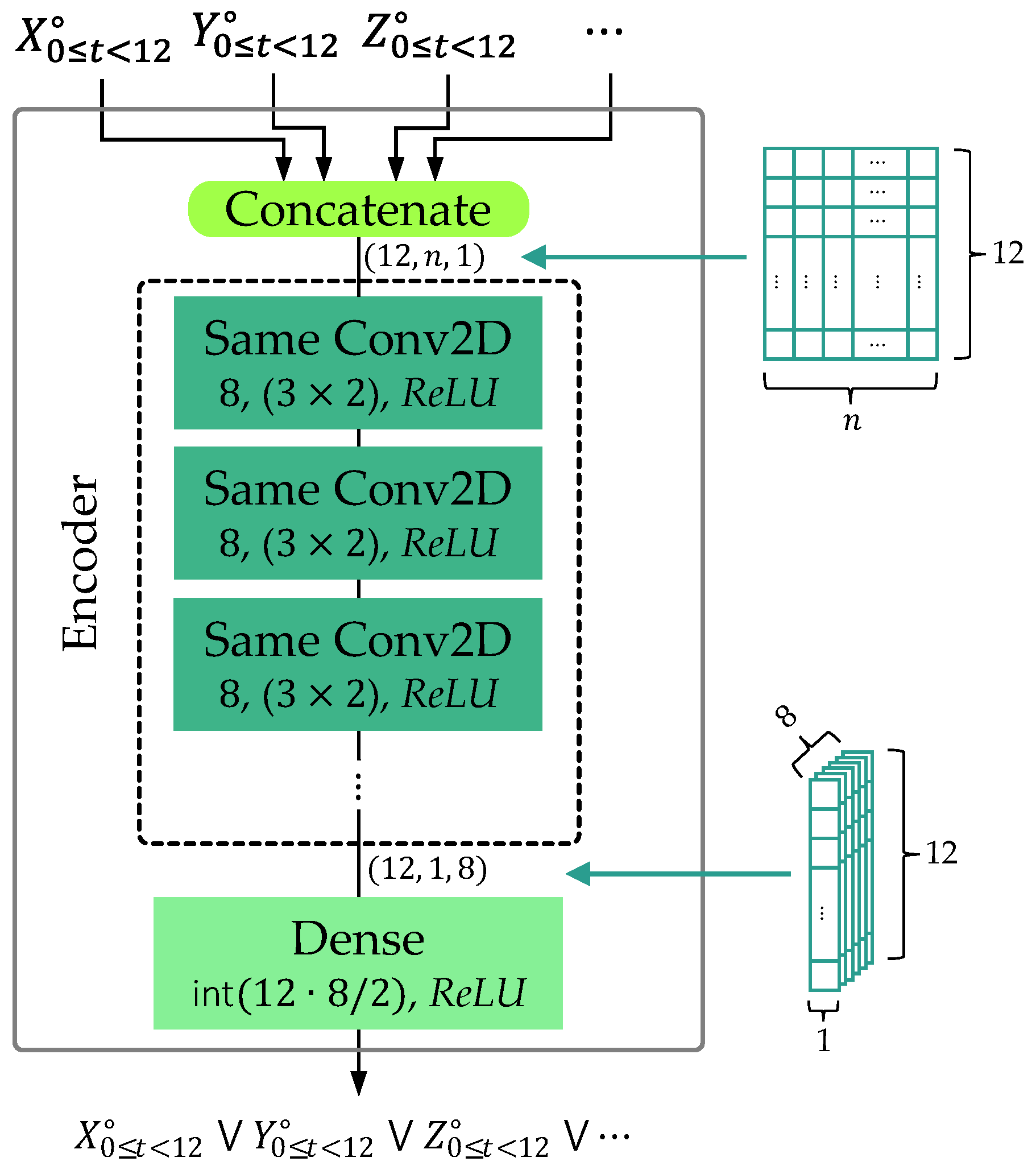
The multivariable ML model used to impute MV or correct AA is shown in Figure 15. The  { m , a } stands for either MV or AA in the data, followed by the number of features as n = [ X , Y , Z , ] , and the sequence length of 0 t < 12 shows the time steps used to rebuild the input data. Depending on the label data used to train, the model can be trained to rebuild specific input. The encoder used a convolutional 2D (Conv2D) layer with custom same padding for maintaining the sequence length and a kernel size of ( 3 × 2 ) . With filter number as 8, the diagonal size of 2 on the kernel reduces the x-axis data size by 1 for each layer, and the layer was repeated until the data condensed from ( 12 , n , 1 ) to ( 12 , 1 , 8 ) . The dense layer with the number of units i n t ( 12 · 8 / 2 ) aggregates and mixes those features across channels to learn global dependencies across the input variables before passing it to the output layer. This ML model used rectified linear unit (ReLU) as the activation function, with the exception of the output layer, where linear was used.
The parameters used to train the ML models are shown in Table 5. Using the Adam optimizer with the learning rate of 0.001, the model was trained using the batch size of 1000 for 300 epochs. To prevent overfitting, the early stop function is deployed to halt the training if the MSE score does not improve by at least 0.001 for 3 consecutive times.
Compared to the MV and AA correction modules that used ML, the CD could be resolved by using a sliding window approach to update the feature scaling with the new data [44,45]. As the electricity load data exhibit similar patterns with different minimum and maximum values, it is effective in addressing the CD without retraining the ML model. This paper expands upon this concept by recalibrating the parameters in the min-max normalization based on the observed minimum and maximum values of each season in the last year, as shown in Figure 16.
By using the previously recorded minimum and maximum values of the same season the ML model is forecasting in the last year, the negative effect from CD could be negated.
Although the modules that impute the MV, amend disturbances from AA, and adjust the scale to counteract CD assist current forecasters in addressing these issues, they fail to recognize that mistakes from earlier modules can accumulate over time. The stacking errors will inadvertently reduce the forecasting accuracy, which the attackers could exploit by performing DDoS attacks to cause MV and adding perturbations via AA when CD occurred due to seasonal changes. To address this issue, the forecaster modules in the stacking operation will compare the pre-correction and post-correction data to forecasts and aggregate the result using a metamodel.

3.2.2. Stack Modules

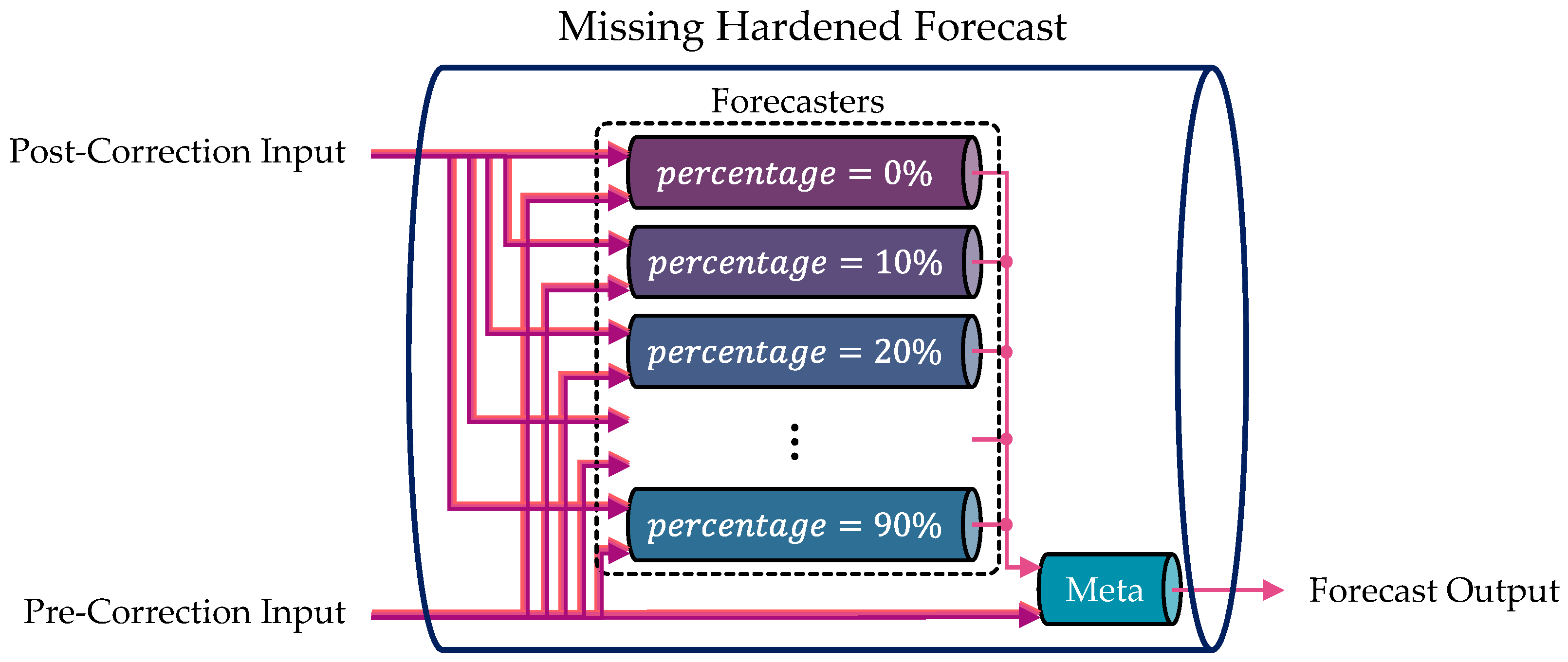
To sort out the imperfection from the MV imputation and adversarial correction, the missing and adversarial hardened forecaster modules compare the pre-correction and post-correction data to identify the changes made and adjust the forecast. The problem with creating a forecaster that could handle a wide range of MV percentage or AA perturbation intensity is the accuracy tradeoff [46]. To address this, the missing and adversarial hardened forecaster modules in the stacking operation also use SEL.
Figure 17 shows the missing hardened forecaster module. Unlike the usual SEL setup, which relies on different types of base models to boost resilience [47], both the base models and the metamodel use the same ML architecture. To induce the heterogeneity and allow the ML models to adjust the forecast based on the pre-correction and post-correction data, each of the base models was trained with different percentages of MV to create variation, followed by the metamodel trained with MV percentages ranging from 0% to 90% to teach it how to adjust the forecast [7].
Similarly, the adversarial hardened forecaster module utilizes SEL configuration that is comparable to the one used in the missing hardened forecaster module, as illustrated in Figure 18. Each of the base models was trained with different perturbation intensity to create heterogeneity, followed by the metamodel trained with perturbation intensity ϵ ranging from 0 to 0.09 to teach it how to adjust the forecast based on the perturbation found.
Base models and metamodels utilized in missing and adversarial hardened forecaster modules use the ML model architecture shown in Figure 19, which expands upon the previous encoder model design in Figure 15. Residual connection was deployed to avoid the vanishing gradient problem due to the number of causal Conv2D layers increasing proportionally as the number of inputs increases. A convolutional 1D (Conv1D) layer with the same padding and a kernel size of 3 was added after the encoder block to prepare the latent representation for future time steps. As the base models, they are trained for prediction. As metamodels, they are trained for adjusting the forecast.
The training parameters are shown in Table 6. The early stop was set to halt the training if the MSE score did not improve by at least 0.0001 for three consecutive times. Though the batch size for the base models does not change, the batch size is cut in half for metamodels to provide more leniency to learn complex patterns.
The drift-hardened forecaster module uses radian scaling to adjust the input without depending on scale, mean, and median values that may vary due to CD [13]. It converts the difference of the p-th discrete difference of an array Δ p X before converting it into radians. However, converting the Δ p X into a radian will yield a bimodal distribution, which requires additional processing. With N as the total number of elements in X, Equation (14) was used to calculate the d i m i n i s h e r value for creating a unimodal distribution in Equation (15).
d i m i n i s h e r = 10 log 10 Δ p X N 1 + 1
X = tan 1 Δ p X d i m i n i s h e r
Figure 20 shows the implementation for the drift-hardened forecaster module, which used radian scaling on the pre-correction data to forecast. The outputs are then unscaled to produce the forecast. The forecaster used the ML model architecture shown in Figure 19.
Finally, the normal forecaster module and the metamodel of the stacking operation reused the ML model architecture in Figure 19, with the same training parameters in Table 6. While the normal forecaster module is trained with normal data, the metamodel is trained with the output from the normal forecaster module, in addition to the MV, AA, and CD hardened forecaster modules. The MV percentage and AA perturbation are proportionally increased when generating the training data.

4. Experiment

4.1. Real-World Dataset

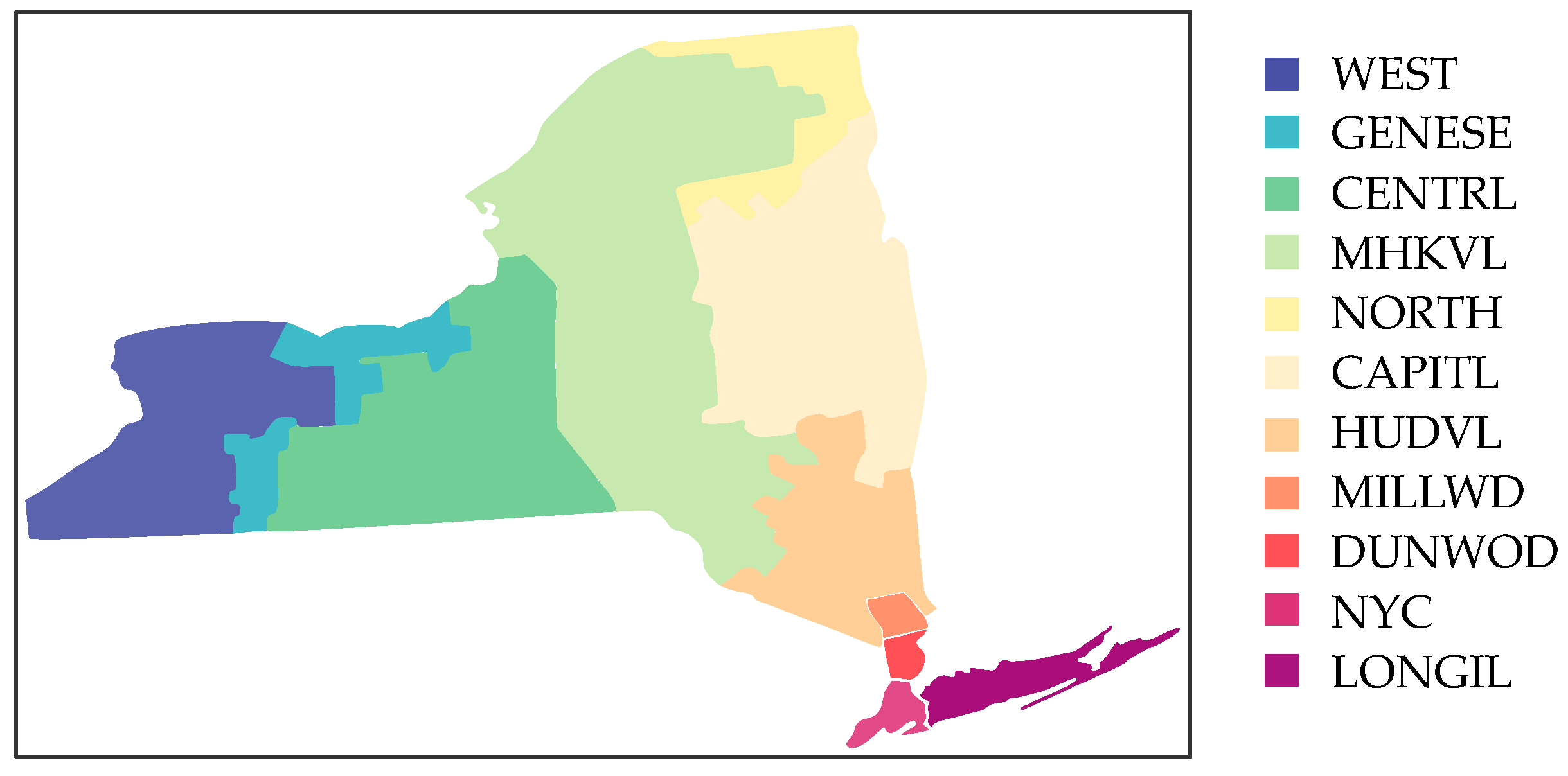
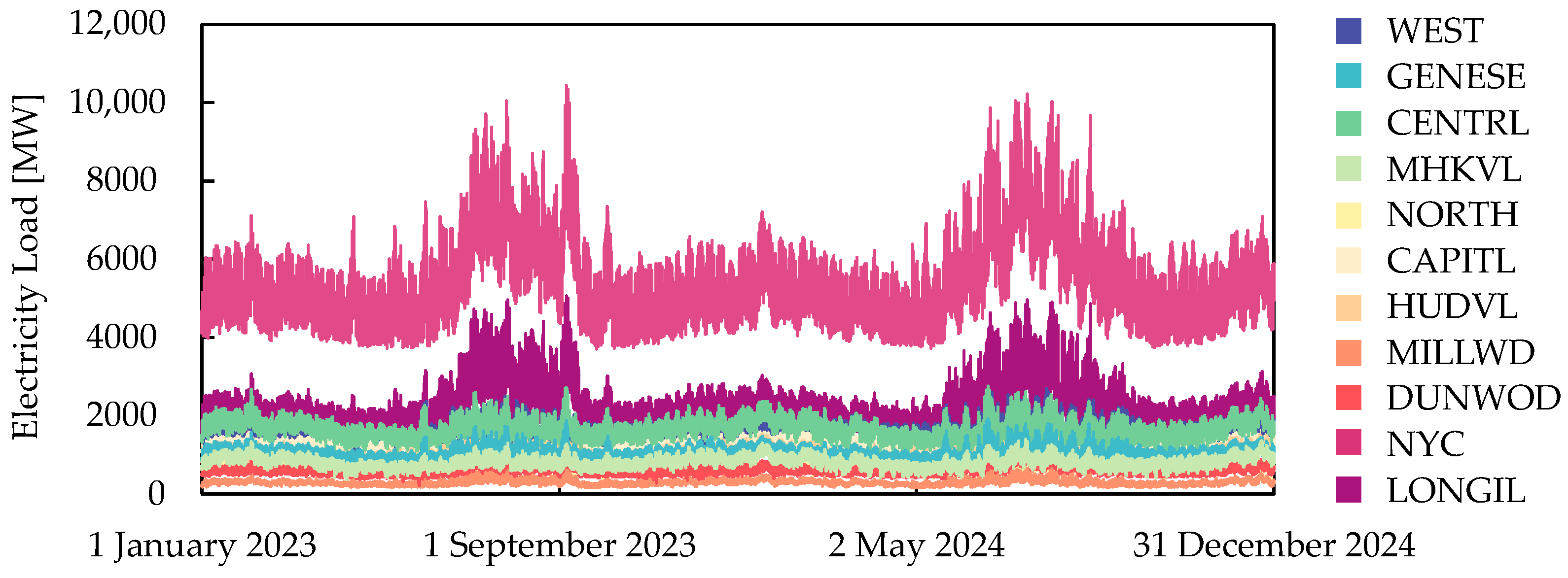
The dataset used in this paper is sourced from the New York Independent System Operator (NYISO) [48], which consists of eleven electricity load zones shown in Figure 21. The load was measured in 5-min intervals from 1 January 2023 to 31 December 2024, and it exhibits upward trends, especially during the summer in Figure 22.
The dataset contains 44 sporadic MV in each zone. To exclude MV from sensors or network issues, imputation was done using Pandas 2.2.3’s polynomial interpolation [49,50] to the order of two. In NYC, there are 7059 outliers found using Statsmodels 0.14.4’s seasonal decomposition set for one week and interquartile range [51,52]. As the outliers represent the real-world trends, no change was made. Figure 23 shows the marked traits.
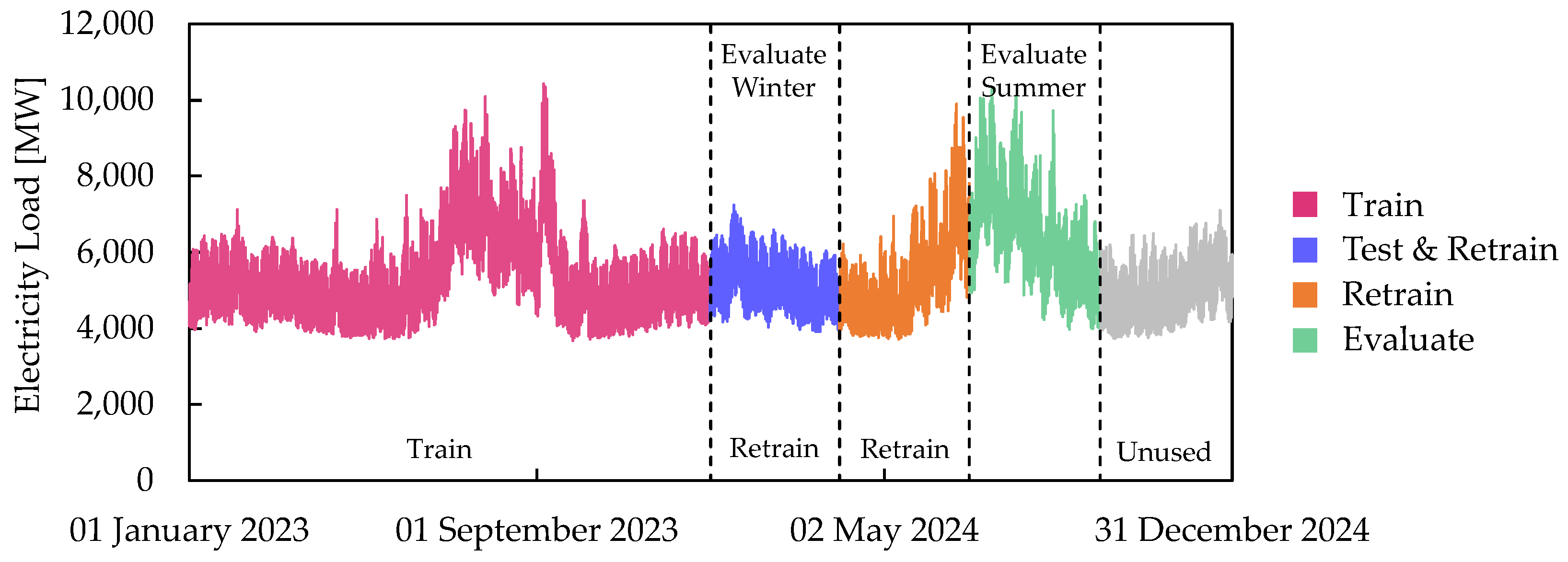
As shown in Figure 24, the electricity load data from 1 January 2023 to 31 December 2023 are used for training. To test the forecaster’s capability to predict the electricity load in NYC, the winter data from 1 January 2024 to 31 March 2024 are used to represent clean data, and the summer data from 1 July 2024 to 30 September 2024 are used to represent seasonal drift data in real-world deployment. Retraining was performed using only the past three months of the previous season to update the forecaster with the latest trends [53].
To find the correlation pairing for the electricity load in the NYC zone, Spearman’s rank correlation coefficient is used because it is helpful even if the data is not normal, contains outliers, or exhibits monotonic relationships [54]. To help with the forecast, only two electricity load data are chosen, as the accuracy gained becomes negligible with more data added. By applying Spearman’s rank correlation from 1 January 2023 to 31 December 2023, DUNWOD and LONGIL are chosen to help the forecast in NYC, as shown in Table 7.

4.2. Proposed Method Application

The proposed StEL implementation was applied to forecast 1 h of electricity load in NYC. As the electricity load data was logged for 5-min intervals, this translates to 12 steps of input taken to forecast the next 12 steps.
Since the StEL implementation described in Section 3 is already established for the experiment, the only remaining task is to sequence the electricity load to match the length that the modules can train and evaluate for accuracy. With selected electricity load as c h o s e n { N Y C , D U N W O D , L O N G I L } and sequence length for the input and output as l = 12 , the data was sequenced using Algorithm 3, with step s = 1 for overlapping training sequences for the model to learn intricate patterns, while s = l for the non-overlapping test sequences for one-on-one comparison with clean data [55].
Algorithm 3 Independent and dependent sequencer
Input: Electricity load data c h o s e n , sequence length l, step s
Output: Independent array i n d e p e n d e n t , dependent array d e p e n d e n t
  1:  Function data _ sequencer ( c h o s e n , l , s )
  2:   Initialize empty arrays: i n d e p e n d e n t , d e p e n d e n t [ ]
  3:    for i = 0 to len ( c h o s e n ) 2 l + 1 step s do
  4:       Append sliced sequence: i n d e p e n d e n t . append ( c h o s e n [ i : i + l ] )
  5:       Append sliced sequence: d e p e n d e n t . append ( c h o s e n [ i + l : i + 2 l ] )
  6:    endfor
  7:   return  i n d e p e n d e n t , d e p e n d e n t
  8: End Function

4.3. Baseline Methods Application

There are two forecasting methods utilized as the baseline to be compared with StEL, which are shown as the following:
  • Trivial solution;
  • Federated solution.
The trivial solution was implemented with the assumption that the data preprocessing could resolve the CD, AA, and CD without facing the stacking errors problem. It relies solely on the cascade operation to correct the issues before passing the corrected input to the forecaster to predict the electricity load, as shown in Figure 25.
The trivial solution used the same training data, test data, sequencer, training strategy, and modules in StEL to measure how effectively the stack operation addressed the stacking errors problem and to compare the results.
The federated solution was implemented based on the federated learning concept and sequence-to-sequence (seq2seq) model used by Yang Zhou et al. [37]. The seq2seq model architecture is shown in Figure 26, which utilizes the previous two hours of historical electricity load ( 24 t < 0 ) and the latest one hour of electricity load data ( 0 t < 12 ) . The LSTM layers are created using 96 units with a TanH activation function, while the sigmoid activation function is applied on the recurrent activation.
This experiment focuses solely on the forecaster’s deployment resiliency, where the dataset used to train the seq2seq in federated learning is clean. This approach is different from StEL and trivial solutions, which purposely add MV and AA to harden the forecast. With a clean dataset, the reputation-based scoring and weighted aggregation are skipped, as shown in Algorithm 4. The dataset used to train the s e q 2 s e q forecaster classes is scaled with min-max normalization d a t a s e t = { D U N W O D , N Y C , L O N G I L } , utilizing the same training parameters in Table 6 to train the local and global models. To resolve the data heterogeneity issue, global models undergo retraining on their corresponding local data to fine-tune the forecast.
Algorithm 4 Federated learning implementation with fine-tuning
Input: Scaled dataset d a t a s e t , untrained model classes s e q 2 s e q
Output: Fine-tuned global models s e q 2 s e q
  1:  Function federated _ learning ( d a t a s e t , s e q 2 s e q )
  2:   Create the list to store the weights: s a v e d _ w e i g h t s [ ]
  3:    for i = 0 to 1 do
  4:        for j = 0 to len ( d a t a s e t ) 1 do
  5:           Get sequence: i n d e p e n d e n t , d e p e n d e n t data _ sequencer ( d a t a s e t [ j ] , 12 , 1 )
  6:           Train the local model: s e q 2 s e q [ j ] . train ( i n d e p e n d e n t , d e p e n d e n t )
  7:           Save the weight: s a v e d _ w e i g h t s . append ( s e q 2 s e q [ j ] . weight ( ) )
  8:        endfor
  9:        if i = 0 do
10:            Average the saved weights: a v e r a g e _ w e i g h t average ( s a v e d _ w e i g h t s )
11:            Replace weight with global: replace _ weight ( s e q 2 s e q , a v e r a g e _ w e i g h t )
12:      endif
13:     endfor
14:    return  s e q 2 s e q
15: End Function

5. Result

Once StEL, the trivial solution, and the federated solution are trained, they are tested to forecast clean data, adversarial data, drifted data, and data with compound problems. For the clean, missing, and adversarial data tests, they are tested on the winter test data that ranged from 1 January 2024 to 31 March 2024. For the drifted data and compounding data, they are tested on the summer data that ranged from 1 July 2024 to 30 September 2024. The seasonal data separation in 3-month intervals will help to identify the strength and weakness of each solution against MV, AA, CD, and compounding problems.

5.1. Clean Data

Table 8 shows the averaged forecasting accuracy metrics where each solution was trained and the accuracies were measured for five times on the winter test data, ranging from 1 January 2024 to 31 March 2024 in NYC. In addition, Table 9 shows the averaged metric differences against Stackade. As the trivial and StEL solutions use the same normal forecasting module configuration, the observed on coefficient of determination ( R 2 ), mean absolute error (MAE), and root mean squared error (RMSE) are the same.
Though the fine-tuning done on the federated solution improved the coefficient of determination ( R 2 ) scores with 1.1974% of difference compared to the trivial and StEL solutions, the averaged MAE score increased from 41.6954 [MW] to 70.7021 [MW], which indicates the federated learning’s forecast is less accurate when compared to the trivial and StEL solutions. Additionally, the averaged RMSE difference of 61.5242% shows the forecast has more outliers when compared to the trivial and StEL solutions.
These results show the accuracy tradeoff for enhancing the privacy in federated solutions [56]. In environments where privacy is not a concern, such as with zonal electricity load data, multivariable forecasting models that rely on centralized learning outperform federated learning. Furthermore, the additional data used in multivariable forecasting models, such as the normal forecaster module, helps the model effectively learn and capture temporal patterns from other zones to improve the forecast in NYC. This tradeoff would be more apparent in the next test when forecasting on MV, AA, CD, and the compounding problems.

5.2. Missing Data

Using the same winter test data, Algorithm 1 was used to randomly replace the electricity load values with MV to simulate the packet loss due to the DDoS attacks. Similar to the test on normal data, each solution was trained five times, and the accuracies were measured to determine the average scores.
While the federated solution uses polynomial interpolation to the order of two to impute MV, the trivial solution uses the imputation module in cascade operation. For StEL, on top of the imputation module in the cascading operation and the missing hardened forecasting module in the stacking operation, the normal forecaster and the meta modules prepared for handling the MV are also deployed to improve the forecasting accuracy under varying MV percentages.
Table 10 shows that R 2 scores on StEL vastly outperformed the federated solution, with the trivial solution slightly lagging behind. This disparity is due to the imputation method deployed in federated learning being limited to only one electricity load data to preserve privacy. In an environment where privacy is not a concern, the additional electricity load data could serve as a reference to enhance the accuracy of imputation, as shown in trivial and StEL solutions.
This observation is confirmed in Table 11 for the averaged MAE scores and Table 12 for the averaged RMSE scores, where the federated solutions have larger MAE and RMSE scores when compared to the trivial and StEL solutions. These results also indicate that the forecast from federated solution is less accurate and has more outliers when compared to the trivial and StEL solutions.
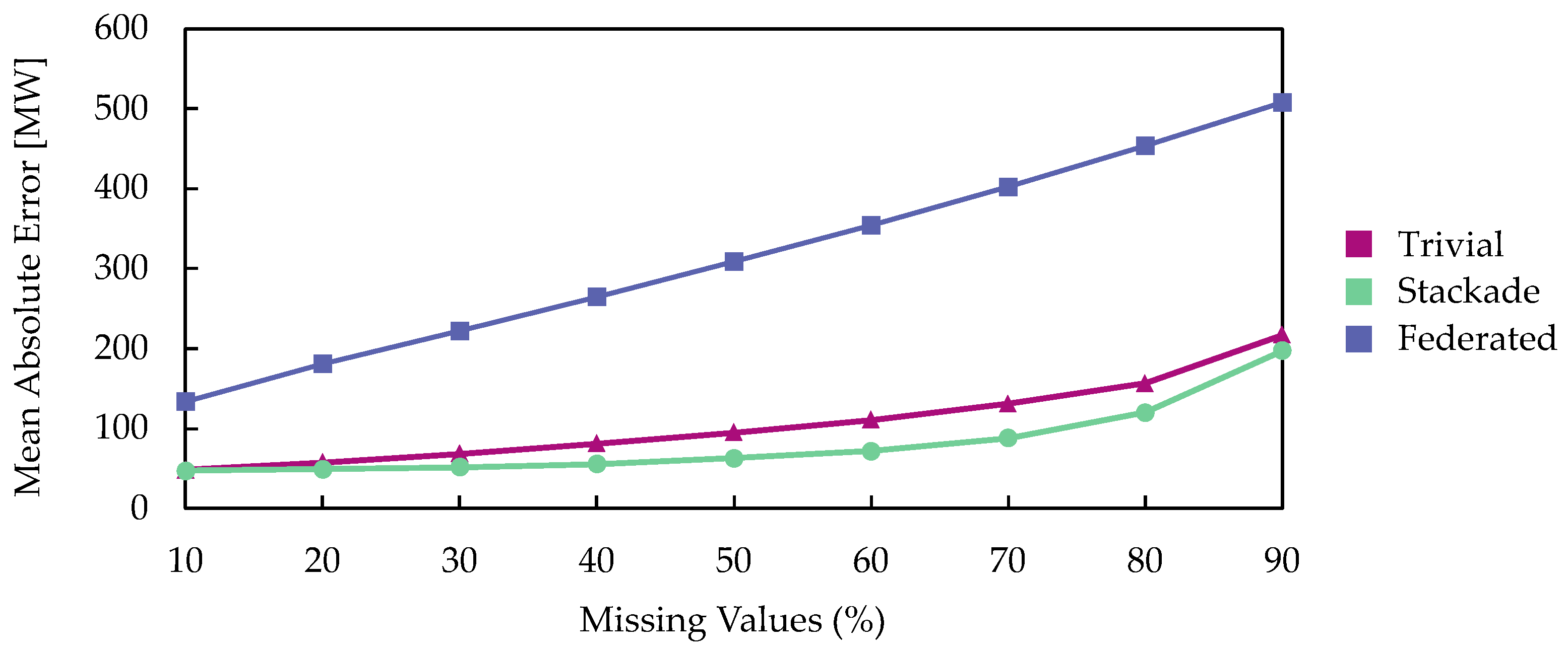
For the trivial solution, the MAE and RMSE scores appear to be slightly lagged behind StEL only when the MV percentage is small or high. This observation can be confirmed by plotting the averaged MAE scores in Figure 27 and by calculating the average MAE difference against StEL in Table 13. While low MV percentages do not show noticeable differences due to both solutions using the same imputation module, in addition to high MV percentages reducing the amount of data needed for the imputation and forecasting to be effective, the StEL solution outperforms the trivial solution when the effectiveness of the imputation module starts to fail.

5.3. Adversarial Data

Using the same data from the winter test, Algorithm 2 was used to insert perturbation. While the adversarial data used to train both the trivial and StEL solutions uses the normal forecaster module to compute the gradient, the perturbation used to measure resiliency uses the surrogate model shown in Figure 28. Although similar to the stacked LSTM model in Figure 8 and using the same training parameters, it was trained with the input and the output of the normal forecaster module from 1 January 2023 to 31 December 2023 to mimic its behaviors and weaknesses [57]. This implementation closely matches the real-world scenarios where the attacker does not have access to the forecaster to create an effective perturbation. Depending on the target models, the surrogate models are configured to be multivariable or univariate models.
Once the solutions and their corresponding surrogate models are trained five times, the averaged accuracies were measured, which are shown in Table 14, Table 15 and Table 16. The results show that without countermeasures to correct the input or harden the forecast in the federated solution, the accuracies will degrade as the ϵ increases.
Although AA effectively reduces forecasting accuracy in the federated solution, both trivial and StEL solutions demonstrate resilience against the attacks. Furthermore, the accuracies between both solutions are almost the same, with StEL having the edge, as shown in the plotted averaged MAE scores in Figure 29 and the averaged MAE differences in Table 17. These results showcase the strength of StEL in enhancing the nearly flawless data correction module by adjusting the forecast to address potential missed corrections. These small improvements are not achievable with the trivial solution, which only performs a single correction to address AA.

5.4. Drifted Data

The experiment on drifted data was tested using summer test data, which ranged from 1 July 2024 to 30 September 2024, for assessing the changes caused by seasonal patterns. This approach is different from the previous experiments that rely on the winter test data to evaluate the performance against normal, missing, and adversarial data. Once the trivial, StEL, and federated solutions were retrained, the accuracies were measured.
Table 18 presents the averaged forecasting accuracies that were repeated five times for data with CD, demonstrating that these solutions achieve high averaged R 2 scores, which indicates they possess strong explanatory power regarding NYC’s electricity load. However, high averaged MAE and RMSE scores on the federated solution show the forecast is less accurate and contains more outliers. Additionally, though the trivial solution has slightly better R 2 scores, StEL has lower averaged MAE and RMSE scores, which shows the forecast is slightly more accurate and has fewer outliers.
In addition to the feature scaling update, the addition of radian scaling and the metamodel to combine the radian and scaled values further reduces the noise in the forecast when compared to the trivial solution. This conclusion is supported by Table 19, where the averaged MAE difference for the trivial and federated solutions is larger than StEL.

5.5. Compounding Data

For the compounding problem, 50% of MV and ϵ = 0.02 for AA were simulated on the summer test data, ranging from 1 July 2024 to 30 September 2024. These values were chosen as the added MV visually hides the perturbation added, which was previously demonstrated in Figure 12 for summer subset data in 2023.
Table 20 shows the forecasting accuracies averaged for five times on the compounding problems. Although the federated solution seems to perform better than the result in Table 10 based on its R 2 score against MV, the MAE and RMSE scores are much larger than the previous test. This result indicates that the federated solution could not capture the overall trend, and the forecasted values significantly deviate from the actual values.
The R 2 score difference between the trivial and StEL solutions is high, which indicates both solutions could capture the overall trend in NYC’s electricity load. However, the averaged MAE score difference for the trivial solution is 30.3783% larger than the StEL solution, as shown in Table 21. This result indicates that the trivial solution is less accurate than StEL. Additionally, the trivial solution has an RMSE score difference of 30.5994% larger than StEL, which indicates that there are more outliers in the trivial solution.

6. Conclusions

As the technologies for forecasting electricity loads mature and see wider deployment in smart grids, the research trend has shifted to focus on enhancing reliability and resiliency against AA. However, because MV and CD are considered extra steps that need to be taken to preprocess the data, the impact of these problems is neglected when dealing with AA. Furthermore, it is difficult to create a solution that not only solves these problems in the data preprocessing stage but also enhances the forecast against them. This weakness could be exploited by malicious actors to enhance the effectiveness of AA in lowering the forecasting accuracy, which could cause inefficient operation that will raise the electricity cost and instability on the smart grid system itself [58].
This paper investigated the limitations of using trivial and federated solutions to resolve the anomalies in the input data due to the MV caused by the DDoS attacks, the AA caused by the hackers, and the CD caused by the seasonal changes. Although a trivial solution that relies on MV imputation, AA correction, and scaling update to resolve CD in a cascading operation could simultaneously handle these issues, the error accumulation from inadequate imputation, correction, or scaling negatively affects the forecasting accuracy. For the federated solution that focuses on safeguarding the forecaster during the training, it faces the data heterogeneity problem in the zonal load in the smart grid environment, causing the forecasting accuracy to degrade and necessitating the global model to be fine-tuned on the local data. Furthermore, as there are no countermeasures to correct AA and update the scale to resolve CD without retraining, it performs the worst when compared to StEL and trivial solutions. Due to the nature of smart grid systems that operate in real-time, this finding on the federated solution’s limitation also highlights the necessity to have multiple countermeasures for handling any type of scenario.
To resolve the limitation in the trivial solution, this paper proposed StEL to combine the strength of cascading operation to resolve the anomalies found in the input data, followed by the stacking operations to identify the inadequate correction done in correcting the input data and adjust the forecast. Although the accuracy gained from resolving only AA and CD is less noticeable, StEL’s capability in handling MV exceeds the trivial solution. Additionally, StEL also outperforms trivial and federated solutions in handling compounded problems with 50% of MV, AA perturbation intensity of ϵ = 0.02 , and seasonal drift. The results highlight the StEL’s strength in addressing the compounding problems.
However, StEL is slow to train and deploy because the metamodel needs to learn the output of each of the base models to make adjustments. For future work, we aim to develop an automated weighted average method that uses reinforcement learning [59] to adjust the weights and transfer learning [60] to shorten the deployment time.

Author Contributions

Data curation, M.H.B.K.; Formal analysis, M.H.B.K.; Funding acquisition, S.Y.; Investigation, M.H.B.K.; Methodology, M.H.B.K. and S.Y.; Project administration, S.Y.; Resources, S.Y.; Software, M.H.B.K.; Supervision, S.Y.; Validation, M.H.B.K.; Writing—original draft, M.H.B.K.; Writing—review and editing, S.Y. All authors have read and agreed to the published version of the manuscript.

Funding

This work was supported by Interface Corporation, Japan.

Data Availability Statement

Data presented in this study are openly available from New York Independent System Operator at https://www.nyiso.com/load-data (accessed on 2 May 2025).

Conflicts of Interest

The authors declare no conflicts of interest.

Abbreviations

The following abbreviations are used in this manuscript:
MLMachine learning
MVMissing values
AAAdversarial attacks
CDConcept drift
DDoSDistributed denial-of-service
AIArtificial intelligence
IoTInternet of Things
NYCNew York City
StELStackade Ensemble Learning
CELCascading Ensemble Learning
SELStacking Ensemble Learning
PGDProjected gradient descent
FGSMFast gradient sign method
BIMBasic iterative method
LSTMLong short-term memory
TanHHyperbolic tangent
MSEMean squared error
GANGenerative adversarial network
DLDeep learning
Conv2DConvolutional 2D
ReLURectified linear unit
Conv1DConvolutional 1D
NYISONew York Independent System Operator
seq2seqSequence-to-seqence
R 2 Coefficient of determination
RMSERoot mean squared error
MAEMean absolute error

References

  1. Ruan, J.; Liu, G.; Qiu, J.; Liang, G.; Zhao, J.; He, B.; Wen, F. Time-Varying Price Elasticity of Demand Estimation for Demand-Side Smart Dynamic Pricing. Appl. Energy 2022, 322, 119520. [Google Scholar] [CrossRef]
  2. Torres, J.F.; Martínez-Álvarez, F.; Troncoso, A. A Deep LSTM Network for the Spanish Electricity Consumption Forecasting. Neural Comput. Appl. 2022, 34, 10533–10545. [Google Scholar] [CrossRef]
  3. Zheng, J.; Du, J.; Wang, B.; Klemeš, J.J.; Liao, Q.; Liang, Y. A Hybrid Framework for Forecasting Power Generation of Multiple Renewable Energy Sources. Renew. Sustain. Energy Rev. 2023, 172, 113046. [Google Scholar] [CrossRef]
  4. Rodrigues, F.; Cardeira, C.; Calado, J.M.F.; Melicio, R. Short-Term Load Forecasting of Electricity Demand for the Residential Sector Based on Modelling Techniques: A Systematic Review. Energies 2023, 16, 4098. [Google Scholar] [CrossRef]
  5. Mohammed, S.; Budach, L.; Feuerpfeil, M.; Ihde, N.; Nathansen, A.; Noack, N.; Patzlaff, H.; Naumann, F.; Harmouch, H. The Effects of Data Quality on Machine Learning Performance on Tabular Data. Inf. Syst. 2025, 132, 102549. [Google Scholar] [CrossRef]
  6. Ahalawat, A.; Babu, K.S.; Turuk, A.K.; Patel, S. A Low-Rate Ddos Detection and Mitigation for SDN Using Renyi Entropy with Packet Drop. J. Inf. Secur. Appl. 2022, 68, 103212. [Google Scholar] [CrossRef]
  7. Bin Kamilin, M.H.; Yamaguchi, S. Resilient Electricity Load Forecasting Network with Collective Intelligence Predictor for Smart Cities. Electronics 2024, 13, 718. [Google Scholar] [CrossRef]
  8. Couldflare. Record-Breaking 5.6 Tbps DDoS Attack and Global DDoS Trends for 2024 Q4. Available online: https://blog.cloudflare.com/ddos-threat-report-for-2024-q4/ (accessed on 16 May 2025).
  9. IBM X-Force. X-Force Threat Intelligence Index 2025. Available online: https://www.ibm.com/reports/threat-intelligence (accessed on 20 May 2025).
  10. Liang, H.; He, E.; Zhao, Y.; Jia, Z.; Li, H. Adversarial Attack and Defense: A Survey. Electronics 2022, 11, 1283. [Google Scholar] [CrossRef]
  11. Bin Kamilin, M.H.; Yamaguchi, S.; Bin Ahmadon, M.A. Leveraging Trusted Input Framework to Correct and Forecast the Electricity Load in Smart City Zones Against Adversarial Attacks. In Proceedings of the 2024 International Conference on Future Technologies for Smart Society (ICFTSS), Kuala Lumpur, Malaysia, 7–8 August 2024; pp. 177–182. [Google Scholar]
  12. Bayram, F.; Ahmed, B.S.; Kassler, A. From Concept Drift to Model Degradation: An Overview on Performance-Aware Drift Detectors. Knowl.-Based Syst. 2022, 245, 108632. [Google Scholar] [CrossRef]
  13. Bin Kamilin, M.H.; Yamaguchi, S.; Bin Ahmadon, M.A. Radian Scaling and Its Application to Enhance Electricity Load Forecasting in Smart Cities Against Concept Drift. Smart Cities 2024, 7, 3412–3436. [Google Scholar] [CrossRef]
  14. Perianes-Rodriguez, A.; Waltman, L.; van Eck, N.J. Constructing Bibliometric Networks: A Comparison Between Full and Fractional Counting. J. Inf. 2016, 10, 1178–1195. [Google Scholar] [CrossRef]
  15. Spodniak, P.; Ollikka, K.; Honkapuro, S. The Impact of Wind Power and Electricity Demand on the Relevance of Different Short-Term Electricity Markets: The Nordic Case. Appl. Energy 2021, 283, 116063. [Google Scholar] [CrossRef]
  16. Li, L.; Ju, Y.; Wang, Z. Quantifying the Impact of Building Load Forecasts on Optimizing Energy Storage Systems. Energy Build. 2024, 307, 113913. [Google Scholar] [CrossRef]
  17. Miller, D.; Kim, J.-M. Univariate and Multivariate Machine Learning Forecasting Models on the Price Returns of Cryptocurrencies. J. Risk Financ. Manag. 2021, 14, 486. [Google Scholar] [CrossRef]
  18. Song, L.-K.; Li, X.-Q.; Zhu, S.-P.; Choy, Y.-S. Cascade Ensemble Learning for Multi-Level Reliability Evaluation. Aerosp. Sci. Technol. 2024, 148, 109101. [Google Scholar] [CrossRef]
  19. Abdellatif, A.; Mubarak, H.; Ahmad, S.; Ahmed, T.; Shafiullah, G.M.; Hammoudeh, A.; Abdellatef, H.; Rahman, M.M.; Gheni, H.M. Forecasting Photovoltaic Power Generation with a Stacking Ensemble Model. Sustainability 2022, 14, 11083. [Google Scholar] [CrossRef]
  20. Djuitcheu, H.; Shah, T.; Tammen, M.; Schotten, H.D. DDoS Impact Assessment on 5G System Performance. In Proceedings of the 2023 IEEE Future Networks World Forum (FNWF), Baltimore, MD, USA, 13–15 November 2023; pp. 1–6. [Google Scholar]
  21. Eliyan, L.F.; Di Pietro, R. DoS and DDoS attacks in Software Defined Networks: A survey of existing solutions and research challenges. Future Gener. Comput. Syst. 2021, 122, 149–171. [Google Scholar] [CrossRef]
  22. Couldflare. DDoS Threat Report for 2025 Q1. Available online: https://radar.cloudflare.com/reports/ddos-2025-q1 (accessed on 4 June 2025).
  23. Chaddad, A.; Jiang, Y.; Daqqaq, T.S.; Kateb, R. EAMAPG: Explainable Adversarial Model Analysis via Projected Gradient Descent. Comput. Biol. Med. 2025, 188, 109788. [Google Scholar] [CrossRef]
  24. Değirmenci, E.; İ, Ö.; Yazıcı, A. Adversarial Attack Detection Approach for Intrusion Detection Systems. IEEE Access 2024, 12, 195996–196009. [Google Scholar] [CrossRef]
  25. Khan, Z.A.; Ullah, A.; Ul Haq, I.; Hamdy, M.; Maria Mauro, G.; Muhammad, K.; Hijji, M.; Baik, S.W. Efficient Short-Term Electricity Load Forecasting for Effective Energy Management. Sustain. Energy Technol. Assess. 2022, 53, 102337. [Google Scholar] [CrossRef]
  26. Hinder, F.; Vaquet, V.; Brinkrolf, J.; Hammer, B. Model-based Explanations of Concept Drift. Neurocomputing 2023, 555, 126640. [Google Scholar] [CrossRef]
  27. Meier, S.; Marcotullio, P.J.; Carney, P.; DesRoches, S.; Freedman, J.; Golan, M.; Gundlach, J.; Parisian, J.; Sheehan, P.; Slade, W.V.; et al. New York State Climate Impacts Assessment Chapter 06: Energy. Ann. N. Y. Acad. Sci. 2024, 1542, 341–384. [Google Scholar] [CrossRef]
  28. Harris, C.R.; Millman, K.J.; van der Walt, S.J.; Gommers, R.; Virtanen, P.; Cournapeau, D.; Wieser, E.; Taylor, J.; Berg, S.; Smith, N.J.; et al. Array programming with NumPy. Nature 2020, 585, 357–362. [Google Scholar] [CrossRef]
  29. NumPy. numpy.histogram. Available online: https://numpy.org/doc/stable/reference/generated/numpy.histogram.html (accessed on 13 June 2025).
  30. Hou, Z.; Liu, J. Enhancing Smart Grid Sustainability: Using Advanced Hybrid Machine Learning Techniques While Considering Multiple Influencing Factors for Imputing Missing Electric Load Data. Sustainability 2024, 16, 8092. [Google Scholar] [CrossRef]
  31. Hwang, J.; Suh, D. CC-GAIN: Clustering and Classification-Based Generative Adversarial Imputation Network for Missing Electricity Consumption Data Imputation. Expert Syst. Appl. 2024, 255, 124507. [Google Scholar] [CrossRef]
  32. Li, D.; Yang, P.; Zou, Y. Optimizing Insulator Defect Detection with Improved DETR Models. Mathematics 2024, 12, 1507. [Google Scholar] [CrossRef]
  33. Zhou, Y.; Ding, Z.; Wen, Q.; Wang, Y. Robust Load Forecasting Towards Adversarial Attacks via Bayesian Learning. IEEE Trans. Power Syst. 2023, 38, 1445–1459. [Google Scholar] [CrossRef]
  34. Mahmoudnezhad, F.; Moradzadeh, A.; Mohammadi-Ivatloo, B.; Zare, K.; Ghorbani, R. Electric Load Forecasting Under False Data Injection Attacks via Denoising Deep Learning and Generative Adversarial Networks. IET Gener. Transm. Distrib. 2024, 18, 3247–3263. [Google Scholar] [CrossRef]
  35. Azeem, A.; Ismail, I.; Mohani, S.S.; Danyaro, K.U.; Hussain, U.; Shabbir, S.; Bin Jusoh, R.Z. Mitigating Concept Drift Challenges in Evolving Smart Grids: An Adaptive Ensemble LSTM for Enhanced Load Forecasting. Energy Rep. 2025, 13, 1369–1383. [Google Scholar] [CrossRef]
  36. Jagait, R.K.; Fekri, M.N.; Grolinger, K.; Mir, S. Load Forecasting Under Concept Drift: Online Ensemble Learning with Recurrent Neural Network and ARIMA. IEEE Access 2021, 9, 98992–99008. [Google Scholar] [CrossRef]
  37. Zhou, Y.; Ge, Y.; Jia, L. Double Robust Federated Digital Twin Modeling in Smart Grid. IEEE Internet Things J. 2024, 11, 39913–39931. [Google Scholar] [CrossRef]
  38. Dorji, K.; Jittanon, S.; Thanarak, P.; Mensin, P.; Termritthikun, C. Electricity Load Forecasting using Hybrid Datasets with Linear Interpolation and Synthetic Data. Eng. Technol. Appl. Sci. Res. 2024, 14, 17931–17938. [Google Scholar] [CrossRef]
  39. Milan Kummaya, A.; Joseph, A.; Rajamani, K.; Ghinea, G. Fed-Hetero: A Self-Evaluating Federated Learning Framework for Data Heterogeneity. Appl. Syst. Innov. 2025, 8, 28. [Google Scholar] [CrossRef]
  40. Alwateer, M.; Atlam, E.-S.; Abd El-Raouf, M.M.; Ghoneim, O.A.; Gad, I. Missing data imputation: A comprehensive review. J. Comput. Commun. 2024, 12, 53–75. [Google Scholar] [CrossRef]
  41. Stevens, A.; Smedt, J.D.; Peeperkorn, J.; Weerdt, J.D. Assessing the Robustness in Predictive Process Monitoring through Adversarial Attacks. In Proceedings of the 2022 4th International Conference on Process Mining (ICPM), Bolzano, Italy, 23–28 October 2022; pp. 56–63. [Google Scholar]
  42. Korycki, Ł.; Krawczyk, B. Adversarial Concept Drift Detection under Poisoning Attacks for Robust Data Stream Mining. Mach. Learn. 2023, 112, 4013–4048. [Google Scholar] [CrossRef]
  43. Alabadla, M.; Sidi, F.; Ishak, I.; Ibrahim, H.; Affendey, L.S.; Ani, Z.C.; Jabar, M.A.; Bukar, U.A.; Devaraj, N.K.; Muda, A.S.; et al. Systematic Review of Using Machine Learning in Imputing Missing Values. IEEE Access 2022, 10, 44483–44502. [Google Scholar] [CrossRef]
  44. Gupta, V.; Hewett, R. Adaptive Normalization in Streaming Data. In Proceedings of the 3rd International Conference on Big Data Research (ICBDR 2019), Cergy-Pontoise, France, 20–22 November 2019; pp. 12–17. [Google Scholar]
  45. Yang, L.; Shami, A. A Lightweight Concept Drift Detection and Adaptation Framework for IoT Data Streams. IEEE Internet Things Mag. 2021, 4, 96–101. [Google Scholar] [CrossRef]
  46. Zhao, S.; Wang, X.; Wei, X. Mitigating Accuracy-Robustness Trade-Off via Balanced Multi-Teacher Adversarial Distillation. IEEE Trans. Pattern Anal. Mach. Intell. 2024, 46, 9338–9352. [Google Scholar] [CrossRef]
  47. Zhang, Y.; Liu, J.; Shen, W. A Review of Ensemble Learning Algorithms Used in Remote Sensing Applications. Appl. Sci. 2022, 12, 8654. [Google Scholar] [CrossRef]
  48. New York Independent System Operator. Load Data. Available online: https://www.nyiso.com/load-data/ (accessed on 2 May 2025).
  49. McKinney, W. Data Structures for Statistical Computing in Python. In Proceedings of the 9th Annual Scientific Computing with Python Conference (SciPy 2010), Austin, TX, USA, 28 June–3 July 2010; pp. 56–61. [Google Scholar]
  50. The Pandas Development Team. pandas.Series.interpolate. Available online: https://pandas.pydata.org/pandas-docs/stable/reference/api/pandas.Series.interpolate.html (accessed on 3 June 2025).
  51. Seabold, S.; Perktold, J. Statsmodels: Econometric and Statistical Modeling with Python. In Proceedings of the 9th Annual Scientific Computing with Python Conference (SciPy 2010), Austin, TX, USA, 28 June–3 July 2010; pp. 92–96. [Google Scholar]
  52. Statsmodels. statsmodels.tsa.seasonal.seasonal_decompose. Available online: https://www.statsmodels.org/dev/generated/statsmodels.tsa.seasonal.seasonal_decompose.html (accessed on 3 June 2025).
  53. Lima, M.; Neto, M.; Silva Filho, T.; de A. Fagundes, R.A. Learning Under Concept Drift for Regression—A Systematic Literature Review. IEEE Access 2022, 10, 45410–45429. [Google Scholar] [CrossRef]
  54. van den Heuvel, E.; Zhan, Z. Myths About Linear and Monotonic Associations: Pearson’s r, Spearman’s ρ, and Kendall’s τ. Am. Stat. 2022, 76, 44–52. [Google Scholar] [CrossRef]
  55. Dehghani, A.; Sarbishei, O.; Glatard, T.; Shihab, E. A Quantitative Comparison of Overlapping and Non-Overlapping Sliding Windows for Human Activity Recognition Using Inertial Sensors. Sensors 2019, 19, 5026. [Google Scholar] [CrossRef]
  56. Wen, H.; Liu, X.; Lei, B.; Yang, M.; Cheng, X.; Chen, Z. A Privacy-Preserving Heterogeneous Federated Learning Framework with Class Imbalance Learning for Electricity Theft Detection. Appl. Energy 2025, 378, 124789. [Google Scholar] [CrossRef]
  57. Zhang, Y.; Song, Y.; Liang, J.; Bai, K.; Yang, Q. Two sides of the same coin: White-Box and Black-Box Attacks for Transfer Learning. In Proceedings of the 26th ACM SIGKDD International Conference on Knowledge Discovery & Data Mining, Virtual Event, 6–10 July 2020; pp. 2989–2997. [Google Scholar]
  58. Maleki, S.; Pan, S.; Lakshminarayana, S.; Konstantinou, C. Survey of Load-Altering Attacks Against Power Grids: Attack Impact, Detection, and Mitigation. IEEE Open Access J. Power Energy 2025, 12, 220–234. [Google Scholar] [CrossRef]
  59. Gao, S.; Zou, Y.; Feng, L. A Lightweight Double-Deep Q-Network for Energy Efficiency Optimization of Industrial IoT Devices in Thermal Power Plants. Electronics 2025, 14, 2569. [Google Scholar] [CrossRef]
  60. Sarmas, E.; Dimitropoulos, N.; Marinakis, V.; Mylona, Z.; Doukas, H. Transfer learning strategies for solar power forecasting under data scarcity. Sci. Rep. 2022, 12, 14643. [Google Scholar] [CrossRef]
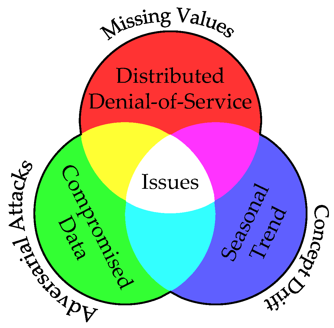
Figure 1. The causes of the missing values, adversarial attacks, and concept drift that could negatively impact the forecasting accuracy.
Applsci 15 08859 g001
Figure 2. The bibliographic analysis identified three clusters, which are technical (green), integration (red), and security (blue).
Applsci 15 08859 g002
Figure 3. The bibliographic analysis identified that trends are shifting from maintaining data quality for basic forecasting to system-level integration, with adversarial attacks gaining traction.
Applsci 15 08859 g003
Figure 4. While the references count from the bibliographic analysis shows fewer studies that match all the keywords, there is only one study that truly unifies the solutions.
Applsci 15 08859 g004
Figure 5. The multivariable forecasting model implemented in smart cities utilizes data from multiple sources to improve the imputation, anomaly correction, and trend adaptation.
Applsci 15 08859 g005
Figure 6. The proposed Stackade Ensemble Learning utilizes cascade to sequentially correct the data and stack to aggregate the forecasts while minimizing the correction errors.
Applsci 15 08859 g006
Figure 7. The comparison between the original electricity load in New York City and the modified time series with 50% of missing values.
Applsci 15 08859 g007
Figure 8. The stacked long-short-term memory forecasting model is utilized as a surrogate model.
Applsci 15 08859 g008
Figure 9. The comparison between the original electricity load in New York City and the modified time series with inserted projected gradient descent perturbation.
Applsci 15 08859 g009
Figure 10. New York City experienced the highest electricity usage during the summer, with similar trends observed in other load zones in New York State.
Applsci 15 08859 g010
Figure 11. The electricity load distribution comparison during the winter, spring, summer, and autumn of 2023 in New York City.
Applsci 15 08859 g011
Figure 12. The comparison between the original drifted electricity load in New York City with the 50% of MV and adversarial perturbation of 0.02 on the electricity load.
Applsci 15 08859 g012
Figure 13. The pre-correction and post-correction input data are parsed for the designated hardened forecaster models to help them identify the inadequate data correction.
Applsci 15 08859 g013
Figure 14. The training order to prepare the solutions for correcting and forecasting the electricity load against missing values, adversarial attacks, and concept drift. The numbers defined the order taken to train the modules.
Applsci 15 08859 g014
Figure 15. The machine learning model used convolutional 2D layer in encoder arrangement to impute or reconstruct the data it was trained with.
Applsci 15 08859 g015
Figure 16. The min-max normalization recalibration utilizes the minimum and maximum values for the same season last year to minimize the negative effect from the concept drift.
Applsci 15 08859 g016
Figure 17. The missing hardened forecast utilized Stacking Ensemble Learning, whereas the base models are trained with different missing percentages to improve the robustness.
Applsci 15 08859 g017
Figure 18. The adversarial hardened forecast utilized Stacking Ensemble Learning, whereas the base models are trained with different adversarial intensities to improve the robustness.
Applsci 15 08859 g018
Figure 19. Expanding upon the previous design, the convolutional 1D layer is added to further condense the representation, followed by the residual connection to stabilize the forecast.
Applsci 15 08859 g019
Figure 20. The forecaster model used radian scaling to scale the data without relying on scale, mean, and median values that could deviate from the training data.
Applsci 15 08859 g020
Figure 21. The New York Independent System Operator partitioned the electricity load in New York State into eleven zones.
Applsci 15 08859 g021
Figure 22. The electricity loads from 1 January 2023 to 31 December 2024 in each zone exhibit seasonal trends, which are prominent during the summer season.
Applsci 15 08859 g022
Figure 23. The two years of electricity load in New York City show sparse missing values with noticeable outliers during the summer season.
Applsci 15 08859 g023
Figure 24. While the dataset for the entire year of 2023 was used for training, the test dataset was set for winter and summer of 2024, with retraining every three months during 2024.
Applsci 15 08859 g024
Figure 25. The trivial solution uses the cascade operation to correct any anomalies found in the input, followed by a normal forecaster.
Applsci 15 08859 g025
Figure 26. The federated solution utilized a sequence-to-sequence model implementation as the local and global models in a federated learning configuration.
Applsci 15 08859 g026
Figure 27. The plotted averaged mean absolute error comparison shows the proposed Stackade Ensemble Learning performed better than the previous and the federated solutions.
Applsci 15 08859 g027
Figure 28. The surrogate model utilizes long short-term memory layer in stacking configuration to emulate the behavior of the target model.
Applsci 15 08859 g028
Figure 29. The plotted averaged mean absolute error comparison shows the addition of historical data used by federated solution negates the negative effect of adversarial attacks.
Applsci 15 08859 g029
Table 1. The comparison between the previous studies highlights the lack of studies that focus on resolving missing values, adversarial attacks, and concept drift.
SolutionAuthorsMissing
Values
Adversarial
Attacks
Concept
Drift
Single-
Purpose
Hou et al. [30]
Hwang et al. [31]
Yihong Zhou et al. [33]
Mahmoudnezhad et al. [34]
Azeem et al. [35]
Jagait et al. [36]
Multi-
Purpose
Yang Zhou et al. [37]✓ *✓ *
* Solution designed to provide protection when training the forecast, not during the deployment.
Table 2. The compatibility issues for each solution against missing values, adversarial attacks, and concept drift.
PrioritySolutionIssues
Missing
Values
Adversarial
Attacks
Concept
Drift
1Impute
2Adversarial Correction
3Scaling Update
While the ✓ represents the issue it can solve, the ✗ represents incompatible problems.
Table 3. The training data used to train the modules within the cascading operation is prepared to teach how to correct the missing values, adversarial attacks, and concept drift.
Cascading ModuleTraining Data
NormalMissing
Values
Adversarial
Attacks
Concept
Drift
Impute
Adversarial Correction
Scaling Update
Table 4. The training data used to train the forecaster modules within the stacking operation is prepared to harden the forecast against missing values, adversarial attacks, and concept drift.
Stacking ModuleTraining Data
NormalMissing
Values
Adversarial
Attacks
Concept
Drift
Missing Hardened Forecast✓ *
Adversarial Hardened Forecast ✓ *
Drift-Hardened Forecast ✓ *
Normal Forecaster
Meta✓ **✓ **✓ **
* Compromised data was preprocessed in cascading operation. ** Compromised data was preprocessed in cascading operation and the forecaster modules in stacking operation.
Table 5. The training parameters used to train the machine learning to impute missing values and correct the perturbation caused by the adversarial attacks.
ParameterValue
Epoch300
OptimizerAdam
Batch Size1000
Early Stop3, 0.001
Learning Rate0.001
Table 6. The training parameters used to train the machine learning to make the forecast more robust or adjust the forecast.
ParameterValue
Epoch300
OptimizerAdam
Batch Sizebase = 1000, meta = 500
Early Stop3, 0.0001
Learning Rate0.001
Table 7. The two highest Spearman’s rank correlation coefficients between other zones and the electricity load in New York City, calculated from 1 January 2023 to 31 December 2023.
ZoneSpearman’s Rank Correlation Coefficient
DUNWOD0.9335
LONGIL0.8787
Table 8. The trivial solution and the Stackade Ensemble Learning have the same accuracy metrics due to using the same normal forecasting module to predict the electricity load.
SolutionAverage Metrics
Coefficient of
Determination
Mean Absolute
Error
Root Mean
Squared Error
Trivial0.992741.695458.3465
Stackade0.992741.695458.3465
Federated0.980870.702194.2437
Table 9. The percentage difference in accuracy metrics of trivial and federated solutions compared to Stackade Ensemble Learning.
SolutionAverage Metrics Difference Against Stackade
Coefficient of
Determination
Δ R 2 (%)
Mean Absolute
Error
Δ MAE (%)
Root Mean
Squared Error
Δ RMSE (%)
Trivial0.00000.00000.0000
Federated−1.197469.568161.5242
Table 10. The averaged coefficient of determination scores under various missing value percentages to simulate the distributed denial-of-service attacks.
Missing Values
(%)
Average Coefficient of Determination
TrivialStackadeFederated
100.98980.99120.9270
200.98560.99060.8674
300.97940.98950.8045
400.97200.98760.7297
500.96230.98350.6458
600.94900.97720.5600
700.93150.96430.4563
800.90520.93280.3453
900.81330.83230.2213
Table 11. The averaged mean absolute error scores under various missing value percentages to simulate the distributed denial-of-service attacks.
Missing Values
(%)
Average Mean Absolute Error
TrivialStackadeFederated
1048.529647.2070133.2267
2057.430349.0083180.9100
3068.663651.9195222.2344
4081.238755.7631264.6083
5095.120662.9048308.5070
60110.910471.7296353.5963
70130.846588.2006402.6867
80156.2930120.3464453.6296
90217.2589197.4284507.5620
Table 12. The averaged root mean squared error scores under various missing value percentages to simulate the distributed denial-of-service attacks.
Missing Values
(%)
Average Root Mean Squared Error
TrivialStackadeFederated
1069.111064.0279184.5113
2081.962366.2038248.5724
3098.043569.9228302.0623
40114.320676.1218355.3547
50132.606787.7459406.9709
60154.3411103.4197453.7577
70178.9805129.3410504.5537
80210.6709177.4555553.7685
90295.7594280.3288603.9647
Table 13. Average mean absolute error difference against Stackade Ensemble Learning under various missing value percentages.
Missing Values
(%)
Average Mean Absolute Error Difference Against Stackade
Δ MAE (%)
TrivialFederated
102.8017182.2179
2017.1848269.1417
3032.2501328.0363
4045.6854374.5219
5051.2136390.4347
6054.6229392.9572
7048.3510356.5576
8029.8692276.9364
9010.0444157.0866
Table 14. The averaged coefficient of determination scores under various perturbation intensity to simulate the adversarial attacks.
Perturbation Intensity
ϵ
Average Coefficient of Determination
TrivialStackadeFederated
0.010.99020.99260.9727
0.020.98860.99100.9491
0.030.98610.98850.9100
0.040.98270.98530.8554
0.050.97820.98100.7853
0.060.97260.97610.6996
0.070.96650.97020.5984
0.080.96010.96520.4817
0.090.95260.95880.3489
Table 15. The averaged mean absolute error scores under various perturbation intensity to simulate the adversarial attacks.
Perturbation Intensity
ϵ
Average Mean Absolute Error
TrivialStackadeFederated
0.0149.308742.857085.7619
0.0254.456547.8518119.6913
0.0361.407155.1187160.4445
0.0469.694262.9749204.3047
0.0579.086672.1098249.7080
0.0689.503481.1657295.9888
0.0799.174690.3727342.7014
0.08108.897098.0133389.7609
0.09118.8386106.0729437.2502
Table 16. The averaged root mean squared error scores under various perturbation intensity to simulate the adversarial attacks.
Perturbation Intensity
ϵ
Average Root Mean Squared Error
TrivialStackadeFederated
0.0167.741059.0411111.4676
0.0272.877764.4952149.4747
0.0380.053572.5370196.1288
0.0488.719681.4213246.6188
0.0598.521491.6195299.1346
0.06109.9490102.3596352.9021
0.07120.8568113.7136407.3712
0.08130.9023121.9266462.2885
0.09141.7989131.6548517.7465
Table 17. Average mean absolute error difference against Stackade Ensemble Learning under various perturbation intensity.
Perturbation Intensity
ϵ
Average Mean Absolute Error Difference Against Stackade
Δ MAE (%)
TrivialFederated
0.0115.0540100.1118
0.0213.8023150.1288
0.0311.4089191.0891
0.0410.6699224.4225
0.059.6753246.2887
0.0610.2725264.6723
0.079.7395279.2088
0.0811.1043297.6613
0.0912.0349312.2168
Table 18. The seasonal shift from spring to summer leads to a drift in the averaged forecasting accuracy metrics.
SolutionAverage Metrics
Coefficient of
Determination
Mean Absolute
Error
Root Mean
Squared Error
Trivial0.996653.734776.7410
Stackade0.996852.538273.6552
Federated0.980870.702194.2437
Table 19. The percentage difference in accuracy metrics of trivial and federated solutions compared to Stackade Ensemble Learning on drifted data.
SolutionAverage Metrics Difference Against Stackade
Coefficient of
Determination
Δ R 2 (%)
Mean Absolute
Error
Δ MAE (%)
Root Mean
Squared Error
Δ RMSE (%)
Trivial−0.02722.27744.1896
Federated−1.578634.572927.9525
Table 20. The compounding problem results show the forecast in each solution exhibits larger errors and more outliers.
SolutionAverage Metrics
Coefficient of
Determination
Mean Absolute
Error
Root Mean
Squared Error
Trivial0.9811132.8607180.2155
Stackade0.9889101.9040137.9911
Federated0.7701456.9376628.6633
Table 21. The percentage difference in accuracy metrics of trivial and federated solutions compared to Stackade Ensemble Learning on compounding data.
SolutionAverage Metrics Difference Against Stackade
Coefficient of
Determination
Δ R 2 (%)
Mean Absolute
Error
Δ MAE (%)
Root Mean
Squared Error
Δ RMSE (%)
Trivial−0.789630.378330.5994
Federated−21.5088348.4002355.5826
Disclaimer/Publisher’s Note: The statements, opinions and data contained in all publications are solely those of the individual author(s) and contributor(s) and not of MDPI and/or the editor(s). MDPI and/or the editor(s) disclaim responsibility for any injury to people or property resulting from any ideas, methods, instructions or products referred to in the content.