A Multi-Task Deep Learning Framework for Road Quality Analysis with Scene Mapping via Sim-to-Real Adaptation

Abstract

Robust perception of road surface conditions is a critical challenge for the safe deployment of autonomous vehicles and the efficient management of transportation infrastructure. This paper introduces a synthetic data-driven deep learning framework designed to address this challenge. We present a large-scale, procedurally generated 3D synthetic dataset created in Blender, featuring a diverse range of road defects—including cracks, potholes, and puddles—alongside crucial road features like manhole covers and patches. Crucially, our dataset provides dense, pixel-perfect annotations for segmentation masks, depth maps, and camera parameters (intrinsic and extrinsic). Our proposed model leverages these rich annotations in a multi-task learning framework that jointly performs road defect segmentation and depth estimation, enabling a comprehensive geometric and semantic understanding of the road environment. A core contribution is a two-stage domain adaptation strategy to bridge the synthetic-to-real gap. First, we employ a modified CycleGAN with a segmentation-aware loss to translate synthetic images into a realistic domain while preserving defect fidelity. Second, during model training, we utilize a dual-discriminator adversarial approach, applying alignment at both the feature and output levels to minimize domain shift. Benchmarking experiments validate our approach, demonstrating high accuracy and computational efficiency. Our model excels in detecting subtle or occluded defects, attributed to an occlusion-aware loss formulation. The proposed system shows significant promise for real-time deployment in autonomous navigation, automated infrastructure assessment and Advanced Driver-Assistance Systems (ADAS).

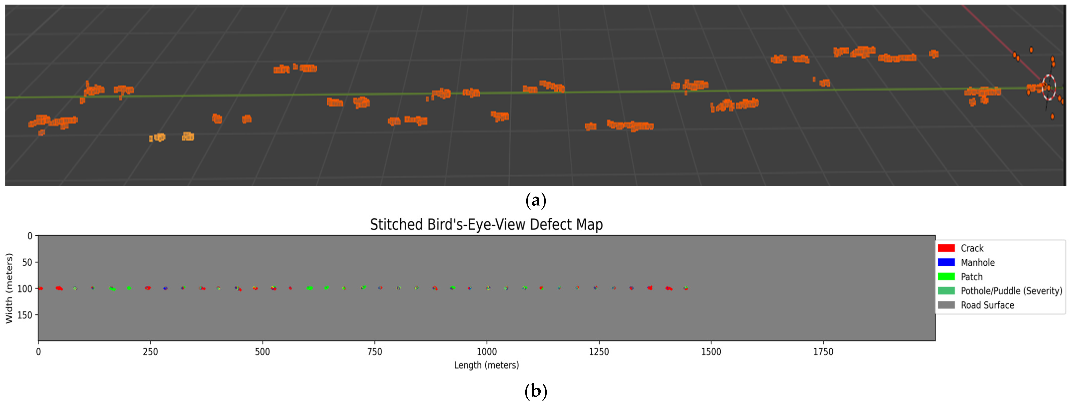
1. Introduction

The development of robust perceptual systems is a cornerstone for advancing autonomous driving and intelligent infrastructure management. A critical component of such systems is the ability to perform accurate and scalable analysis of road surface quality. Road defects, such as cracks and potholes, present substantial obstacles; significant damage can impede vehicle development, while even minor flaws can cause path deviations at high speeds, increasing the probability of accidents [1,2,3]. Consequently, ensuring that autonomous navigation systems can consistently find and respond to surface problems is a top safety priority, as emphasized by transportation authorities who develop detailed guidelines for pavement assessment [4]. Traditional manual inspections are expensive, time-consuming, and not always accurate [5]. However, the rise in sensor data from connected and autonomous vehicles (CAVs) makes it possible to perform automated, data-driven evaluations.

Early automated systems used traditional computer vision, while newer supervised deep learning models [6] depend on vast, carefully annotated datasets for their performance. It is well known that collecting and labeling real-world road problem data by hand is very time-consuming, expensive, and difficult to accomplish in a way that captures all the many types of environmental conditions and defects. Synthetic data production has become a powerful and feasible alternative to overcoming these data collecting challenges. It gives you complete control over how data is made and comes with accurate, automatically created ground-truth annotations [7].

This work builds on this idea by creating a complete system for analyzing road quality, based on a new, procedurally created synthetic dataset. We used Blender to make a detailed 3D environment that has not only ordinary road problems like cracks, potholes, patches, and puddles, but also important road furniture like manhole covers. Our pipeline creates comprehensive ground-truth data, such as semantic segmentation masks, depth maps, and camera characteristics (both intrinsic and extrinsic). This helps us grasp the picture better than just segmentation alone. The problem with training on synthetic data, though, is the synthetic-to-real (sim-to-real) domain gap. This research focuses a lot on closing this gap with a complex two-stage domain adaptation technique. We initially use a new segmentation-aware CycleGAN to translate images in a way that keeps the geometric accuracy of small faults. Then, while training the model, we use a dual-discriminator adversarial learning strategy that aligns the feature and output distributions. This makes the domain shift even smaller.

However, standard image-to-image translation methods often fail to preserve the fine-grained geometric details of small road defects, sometimes degrading or removing them entirely. Our work directly addresses this by introducing a novel segmentation-aware loss into the CycleGAN framework, which explicitly enforces defect fidelity during translation. Furthermore, while prior multi-task models exist, few integrate segmentation, depth, and camera parameter estimation in a way that ensures geometric consistency for 3D reconstruction from a single image. Our framework is the first to combine these tasks with a dual-discriminator domain adaptation strategy, creating a comprehensive system that is robust, efficient, and capable of a rich 3D semantic understanding of the road scene.

Our main contributions are as follows:

• We present a large-scale, procedurally generated synthetic dataset for multi-task road quality analysis, featuring diverse defects with dense, pixel-perfect annotations for segmentation, depth, and camera poses.
• We propose a multi-task deep learning framework that jointly predicts discrete-defect masks, continuous severity maps, depth, and camera parameters, enabling comprehensive 3D reconstruction from images.
• We introduce a novel two-stage domain adaptation pipeline, combining a segmentation-aware CycleGAN for image translation with a dual-discriminator adversarial network for in-training feature alignment.

2. Related Work

The automated detection of road defects has transitioned from traditional image processing techniques to deep learning-based approaches. Early methods using thresholding, edge detection, or engineered features generally had trouble since road conditions changed so much in the actual world [8]. Deep learning, especially Convolutional Neural Networks (CNNs), set a new standard by automatically learning strong feature representations [9].

It did not take long for semantic segmentation architectures to be modified to suit this task. Foundational models like Fully Convolutional Networks (FCNs) and U-Net did well because they could produce dense, pixel-level predictions. For example, FCN-based models were made just for finding small cracks [5,10], and U-Net-based designs have been shown to work well for finding many sorts of defects at the same time [11]. Later improvements led to more powerful architectures, such as PSPNet [12], Feature Pyramid Networks (FPN) [13], and DeepLabv3+ [14]. These techniques utilize multi-scale feature fusion and atrous convolutions to enhance accuracy, particularly for minor or irregularly shaped defects [15]. More recently, advanced models have integrated transformer-based attention mechanisms with multi-scale feature aggregation to further boost performance on complex pavement textures [16]. Some studies have successfully used Deep CNNs on specific data sources, like employing laser-scanned range images to classify cracks with high accuracy [17].

Single-task segmentation is effective, but multi-task learning (MTL) has emerged as a powerful approach for constructing more comprehensive and reliable models. This has led to models that combine semantic comprehension with geometric reasoning in the study of road scenes.

Several studies have shown that predicting depth and segmentation together gives better results by making sure that the geometry is consistent [18]. Building on this, recent works have focused on integrating depth information into more comprehensive scene understanding tasks, such as panoptic segmentation, which unifies both semantic and instance-level recognition [19]. This makes it possible to identify flaws and measure their severity in numerical terms. More advanced models now include surface normal prediction to better capture the orientation of 3D surfaces, which is especially helpful in complicated lighting [20]. Recently, researchers have looked into how to explicitly predict the intrinsic and extrinsic properties of a camera to put 2D predictions into a metrically precise 3D context, which allows for the creation of detailed 3D defect maps [21]. Even so, a lot of the current research focuses on finding and classifying defects, and it typically does not go into enough detail about measuring defect characteristics like width or severity [22,23].

Along with MTL, another area of research is multi-modal sensing. Some methods use unmanned aerial vehicles (UAVs) with sensors like LiDAR and optical cameras for crack inspection [24,25]. Combining LiDAR point clouds and camera images, with the proper extrinsic sensor calibration, has also been proposed as a new way to make automated 3D crack models. These studies show that there is a strong trend toward using additional data sources to obtain a better picture of the road environment.

The necessity for vast amounts of carefully labeled data is a significant problem for all supervised deep learning approaches. Synthetic data production has become a meaningful way to overcome the challenge of high cost and time needed to obtain real-world data, allowing for the creation of controlled datasets with excellent ground truth for a wide range of defect types and conditions.

But this brings up the critical problem of the synthetic-to-real (sim-to-real) domain gap. So, domain adaptation methods are pretty important. CycleGAN [26] is a well-known approach for unsupervised image-to-image translation and has worked well in several self-driving situations [27,28]. CycleGAN-based methods have shown potential in making synthetic images look more like actual ones in the area of road faults, which makes it easier for trained models to be transferred [29]. Adversarial domain adaptation during training is a second strategy that is typically used in conjunction with the first. It uses a domain discriminator to make the model learn features that are not specific to any one domain [9].

There are still essential gaps, even with these improvements. First, not many frameworks can manage both discrete flaws (like cracks, which need binary masks) and continuous faults (like potholes, which need ranging severity/depth masks) in the same output. Second, while MTL is being studied, most existing models do not combine all of the outputs—segmentation, depth, and camera parameters—in a way that ensures the geometry is consistent for strong 3D reconstruction. Finally, CycleGAN is an excellent tool for style transfer, but conventional implementations lack sufficient flexibility, which can exacerbate the problems they aim to address or even eliminate. Our work directly addresses these problems. We propose a comprehensive framework capable of predicting multiple tasks with discrete, continuous, and geometric outputs, while also incorporating a novel two-stage domain adaptation technique. Our segmentation-aware CycleGAN ensures that defects remain unchanged during translation. At the same time, our dual-discriminator adversarial training makes the domains more similar to each other, resulting in a model that is both thorough in its comprehension and strong in its real-world applications.

3. Synthetic Dataset Generation for Road Defect Analysis

It is challenging to develop robust and generalizable deep learning models for detecting and distinguishing road defects due to the scarcity of real-world datasets with extensive annotations. To make this problem more straightforward to deal with, a pipeline for creating synthetic datasets has been made that uses a 3D modeling and rendering environment (Blender 4.3+) and Python 3.9 scripting to automatically build up scenes, generate data, and create complete ground-truth labels. This method enables precise adjustment of scene parameters, environmental circumstances, and defect characteristics, resulting in a wide range of data with pixel-perfect ground truth labels. This solves the problems that come with collecting data in the actual world.

3.1. Three-Dimensional Scene Construction and Road Modeling

The synthetic dataset is constructed within a meticulously designed 3D environment that depicts various road networks in urban environments that evolve. Utilizing Blender’s Bezier curve tool, which allows for the parametric representation of a road’s trajectory, you may establish the primary road framework. This curve, designated as “road,” is crucial for the movement of the camera and other objects along its trajectory. Subsequently, the road mesh acquires a sophisticated physically based rendering (PBR) asphalt material, created in Blender through a node-based shader network. This substance resembles authentic asphalt or concrete textures. The process begins with Texture Coordinates and Mapping nodes to establish the UV coordinate space for accurate texture alignment. High-resolution Image Texture nodes (4K) provide albedo maps featuring various wear patterns. The Roughness and Normal Texture nodes introduce minute characteristics to the surface, such as tire marks and gravel particles. A Perlin noise texture is incorporated to introduce randomness in the scaling and rotation of the texture, hence preventing the repetition of patterns across extensive areas. A Principled Bidirectional Scattering Distribution Function (BSDF) shader utilizes the output from these texture nodes to regulate surface defects and specular highlights. Displacement and Bump nodes are used to modify the geometry of the road mesh, introducing minor height variations to enhance realism and reduce perfection. This base material is designed to be modular, facilitating the incorporation of modifications specific to defects. The scene is rendered swiftly and effortlessly using Blender Eevee Cycle with suitable sampling values. 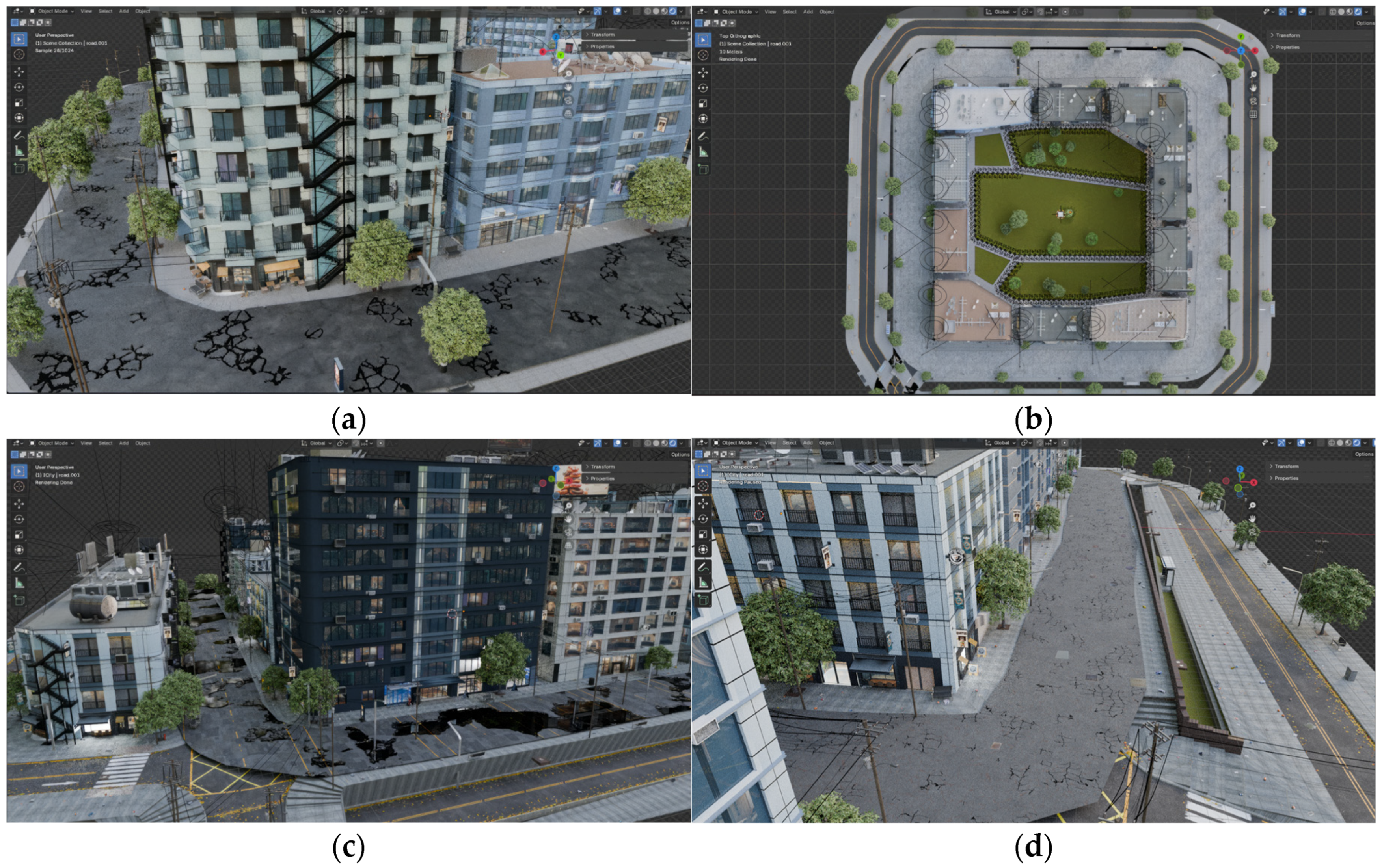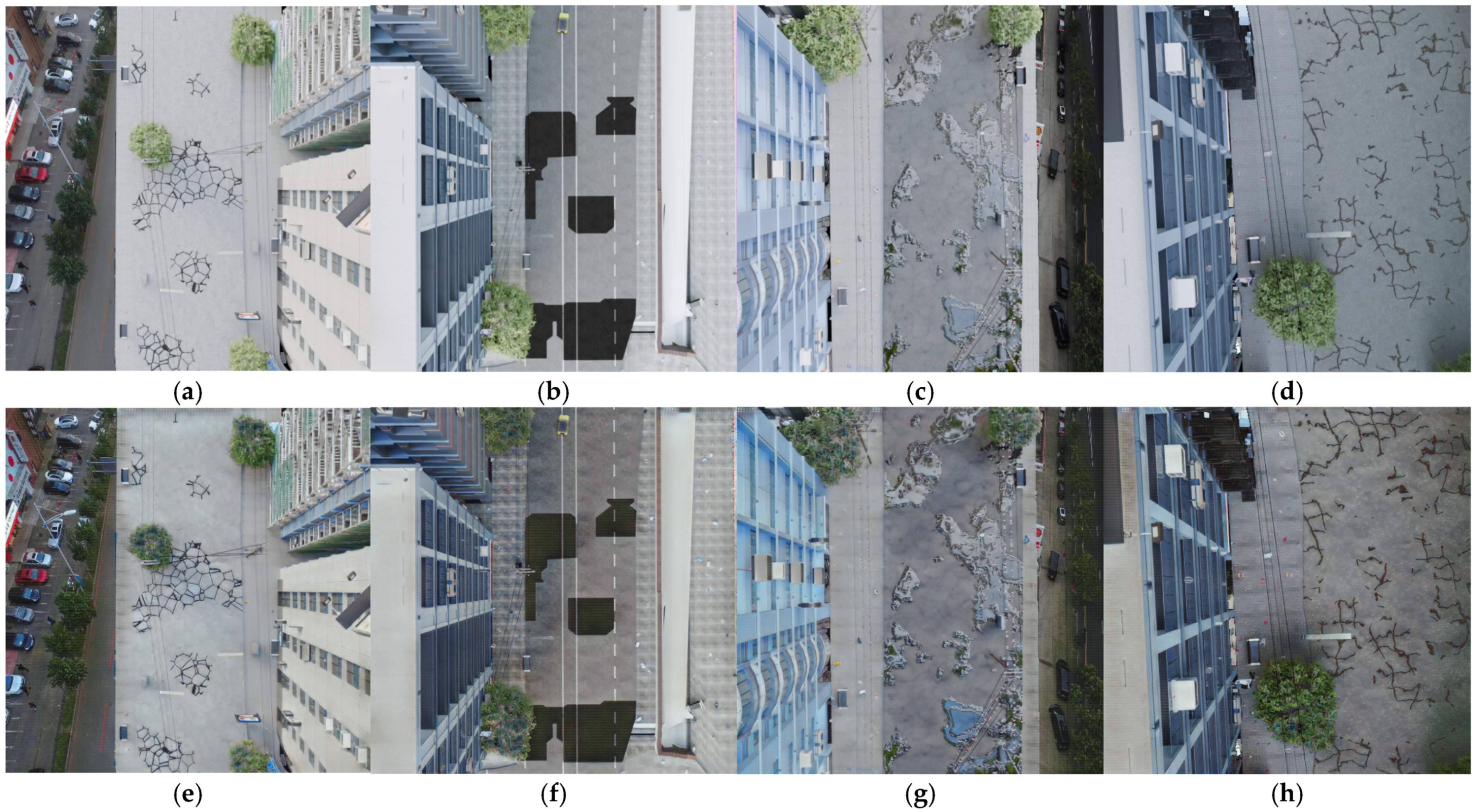Figure 1 illustrates some of the 3D scenes created using Blender.

3.2. Defect-Specific Modeling and Integration

A critical and innovative aspect of this synthetic pipeline is the detailed procedural modeling and integration of various road defects, ensuring high fidelity and precise control over their characteristics:

3.2.1. Cracks

Using a mix of Wave Texture and Color Ramp nodes, crack patterns can be created. The Wave Texture node can make either vertical or horizontal sinusoidal waveforms. The Scale parameter controls the density of the cracks, while the Distortion parameter adds irregularity. After that, the Color Ramp node takes the output from the Wave Texture and turns the waveform into a binary mask, which clearly shows where the cracks are. Using a Mix Shader, this binary mask is then mixed with the base asphalt material. The fissures are given a lower roughness and a darker albedo to make them look like dirt has built up inside them. A Displacement Modifier provides the crack with mesh geometric depth by pushing it out by 1 to 5 cm based on a grayscale depth map made from the crack mask. A Bump Node enhances perceptual depth without altering the existing mesh geometry.

3.2.2. Potholes

Boolean operations are used to subtract cubic volumes from the road mesh to create potholes. After the Boolean operation, dynamic topology sculpting tools are used to smooth out the edges of the holes that were just made. They also add realistic debris and irregularities around the edges. Using a Mix Shader node, the material in the potholes is then mixed with the underlying road material. This adds specific wet or dirty textures to make the holes look more like those under real-world conditions. Voronoi textures can also be used to create polygonal patterns that indicate the locations of potholes. To make different irregular forms, the scale and randomization settings on the Voronoi Texture node are changed. Using math operations like addition and multiplication, these patterns are paired with Noise Texture nodes to create faulty geometries that vary each time. A Bump node is also used to change the depth of the potholes on the road.

3.2.3. Patches

To simulate repaired asphalt areas, we procedurally generate road patches primarily through the use of Voronoi Texture nodes, which can be configured to produce square, rectangular, or irregular shapes. To achieve more complex and randomized patch geometries, we employ Math Nodes to perform addition and multiplication operations, thereby combining multiple Voronoi cells. To ensure the patches appear naturally integrated into the surrounding road, we simulate edge wear and realistic blending by using a Noise Texture. This texture drives variations in roughness within the patch material, preventing the appearance of artificially perfect geometric shapes. Furthermore, by combining these Voronoi patterns with Noise Textures and Bump nodes, we can create patches that are slightly elevated or that exhibit varied surface textures, closely mimicking the appearance of real-world road repairs.

3.2.4. Puddles

Puddles, emulating water-filled depressions, are created with a Glass BSDF shader to precisely mimic light refraction and specular reflections, yielding a realistic water appearance. The configurations of puddles are determined using Gradient Texture nodes, adjusted by Color Ramp modifications, resulting in circular or elongated shapes. A Gradient Texture regulates depth variation inside the puddle, resulting in a deeper appearance at the center compared to the edges. Surface ripples are emulated by Normal Map nodes influenced by artificial noise, while Geometry Nodes can be employed to delicately move vertices, producing shallow depth gradients that augment realism. Dynamic Paint is utilized to generate ripple effects during rainfall in dynamic scenes, thereby augmenting environmental realism.

3.2.5. Manhole Covers

To represent common elements of urban infrastructure, we place manhole covers throughout our scenes. We start by importing pre-made 3D models, which are flexible enough to let us adjust their key features. For instance, we can change their diameter to anywhere between 60 and 120 cm, switch their material between cast iron and concrete, and set them to be either flush with the road or sticking out slightly using bump nodes. To make them look like they are genuinely part of the road, we use a Boolean tool to essentially cut their geometry out of the road’s surface, creating a perfectly shaped recess for the cover to sit in. We then apply a material that combines metallic roughness with ambient occlusion maps to give the manholes a highly realistic appearance.

3.3. Scene Composition and Variability (Domain Randomization)

We enrich our scenes with a wide range of characteristics and changing surroundings to make our synthetic data as realistic as possible, ensuring the models we train on it can handle real-world conditions. We use high dynamic range photos, High Dynamic Range Image (HDRI) as a background and randomly rotate and change the intensity and color to make it look like different times of day, from dawn to twilight. The cityscapes around it are also made in real time. With Blender’s City Builder add-on, we can sometimes create whole cities, with buildings, sidewalks, and plants, all at once. Sometimes we utilize Blender GIS to bring in real road layouts from OpenStreetMap and then add more buildings and plants to them. We use custom Python functions to place 3D models of automobiles on the road randomly. This helps the model to learn the road defects even in the presence of vehicles. We adjust the number of cars on the corresponding routes to simulate real-life scenarios where other vehicles might obstruct the view. We also strategically place cars in specific locations to mask certain road flaws, allowing our model to learn how to handle unclear information using an occlusion-aware mask. 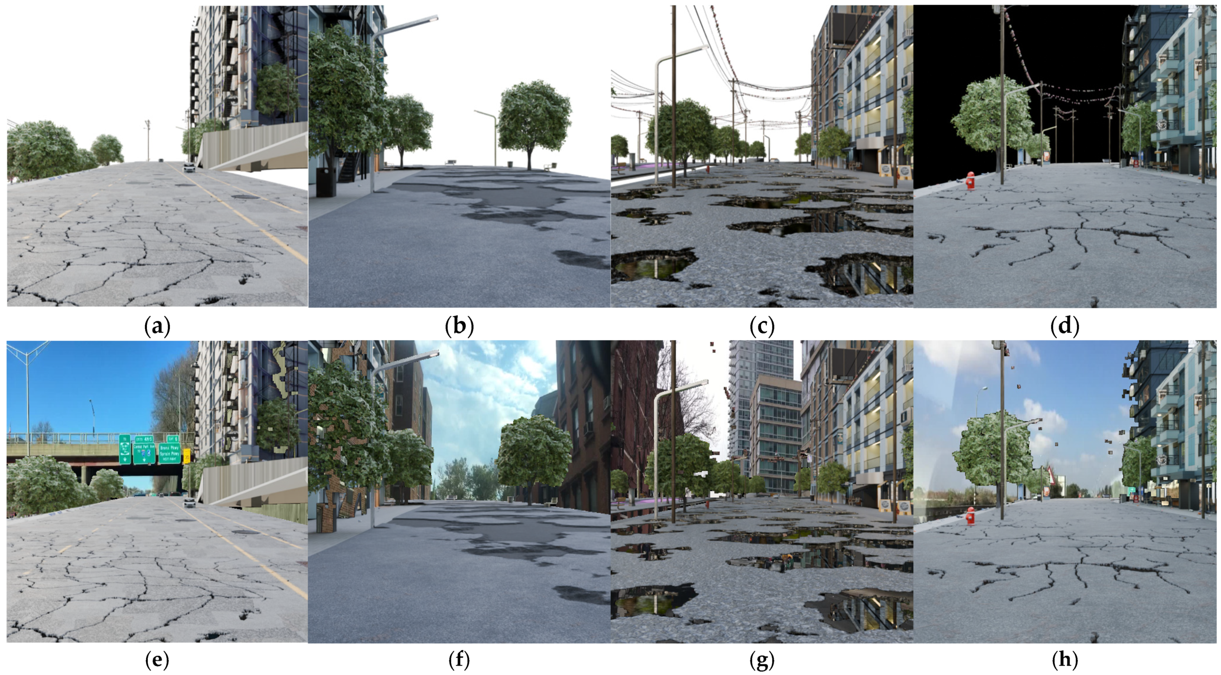Figure 2 illustrates some of the 3D scenes with random road textures and car models placements created using Blender. The defect seed is kept constant to show various-texture-based randomization. Still, while rendering the dataset, the noise texture seeds are changed to obtain a wide variety of crack visuals for a single scene.

3.4. Camera System and Trajectory Generation

To generate our synthetic data, we use a dynamic camera system that mimics the movement of cameras mounted on land and aerial vehicles. The camera’s path is guided by a Bezier curve that defines the road and flight path, giving us precise control over its position and angle. Through a Python script, we can easily configure key settings to alter the viewpoint. For example, we can adjust the camera’s height from the road surface, its lateral position away from the centerline, and its distance from the point it is looking at. We also control a look-ahead factor, which determines how far down the road the camera focuses. For every frame we generate, we calculate the camera’s exact position, tangent, and normal vectors along the road’s curve. This ensures the camera smoothly follows the road’s turns and elevation changes, allowing us to systematically capture a wide range of perspectives and environmental conditions along the entire stretch of the road, which is essential for training dependable perception models for real-world use.

3.5. Automated Rendering Pipeline and Label Generation

We developed a powerful batch rendering system using Blender’s Python API to fully automate the creation of scenes and the exportation of data. With every new image, the script introduces variety by randomly altering the types and characteristics of road defects, lighting, camera, and vehicle placements. This process generates a synchronized set of images and perfectly accurate ground-truth labels. The data package for each scene is comprehensive. It starts with a high-resolution RGB image, which is the primary input for our models. Alongside this, we export a detailed 32-bit depth map in EXR and PNG format, providing exact distance information for every pixel. Critically, the system produces pixel-perfect segmentation masks that identify each type of defect, such as cracks, potholes, or patches, and also outline dynamic objects like cars to account for anything blocking the view.

To support applications that need a deep geometric understanding, like simultaneous localization and mapping (SLAM), all camera-specific details, including focal length and position, are carefully logged in JSON files. A photorealistic color image is rendered using Blender’s EEVEE or Cycles engine. Simultaneously, a corresponding depth map is extracted from Blender’s Z-buffer using the compositor. This depth data is normalized to a 0–1 range and saved as a 16-bit PNG to preserve high precision, providing dense geometric information for every pixel. For each rendered frame, we calculate and save the complete camera model. This includes the 3 × 3 intrinsic matrix (K), which contains the focal length and principal point, and the 3 × 4 extrinsic matrix (R), which defines the camera’s 6DoF pose (position and orientation) in the world coordinate system. These parameters are serialized to a JSON file, providing perfect ground truth for tasks involving camera pose estimation or 3D reconstruction. The generation of defect masks is achieved through a novel, material-based rendering approach. Rather than drawing masks, we manipulate the road’s shader node tree in Blender.

For classes like cracks, manhole covers, and patches, a specific texture or procedural noise node within the road material is isolated and connected to the material’s output. The scene is then rendered, producing an image where only that specific defect feature is visible. This output is thresholded to create a clean binary mask. These binary masks are then composited into a single semantic label map, where pixel values are assigned a specific integer ID (30 for cracks, 60 for manholes, 90 for patches). For defects like potholes and puddles, where severity or depth is essential, the exact material-based rendering is used. However, instead of a binary output, the grayscale intensity from the corresponding shader node depth is remapped to a specific integer range (100–200). This directly encodes a measure of severity into the final label map, providing richer information than a simple binary mask.

3.6. Dataset Details

To effectively train and test our system, we built a robust data pipeline. This involved creating a new synthetic dataset from scratch for initial training and then using carefully selected real-world images to help the system adapt. This dataset contains 16,036 high-resolution (512 × 512) images and label pairs, offering a detailed environment for learning to understand road scenes. We split the data for two different camera views. The first is a dashcam view consisting of 6331 images for training and 1582 for validation. The second is a drone view comprising 6491 images for training and 1623 for validation. Our process focused on generating a wide variety of realistic road environments that include five common types of road damage: cracks, potholes, puddles, patches, and manhole covers.

We also introduced a unique background augmentation method. Our procedurally generated scenes mainly included the road and nearby objects like buildings and cars, leaving the sky or distant background empty. To make the images more realistic and prevent our model from taking shortcuts, we automatically filled these empty areas with backgrounds from real domain photos. This creates a complete and realistic scene for training. To close the gap between our synthetic data and what the system will see in the real world, we used two well-known public datasets. We only used the daytime images from these datasets to serve as a style guide for our image translation model. For the dashcam perspective, we turned to the Berkeley Deep Drive BDK100 dataset. We first sampled only the daytime images from 36,728 images to avoid day-night complex style translations, which might cause domain confusion. Then, we sampled a smaller, high-quality set of 6331 images to match a 1:1 ratio with our synthetic training data. We gave our CycleGAN a focused target, allowing it to learn diverse, real-world styles without getting thrown off by the larger dataset’s specific look. For the drone view, we used the VisDrone dataset. We followed a similar process, filtering its 4350 images to remove night scenes. We then used this entire subset as our target, keeping a rough 1:1 ratio with our synthetic drone images. This gave us a consistent and representative style for adapting our aerial photos.

4. Proposed Method

4.1. Overall Architecture

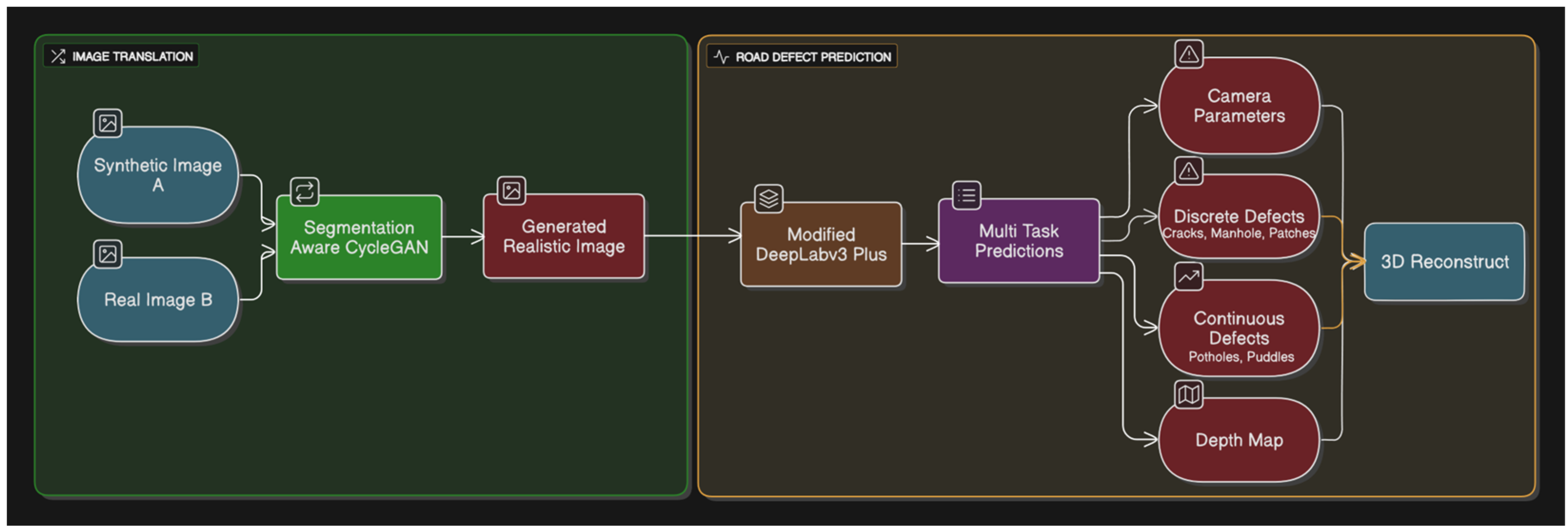
This study introduces a novel two-stage deep learning architecture for comprehensive road monitoring, designed to simultaneously perform discrete-defect detection, continuous severity estimation, depth map prediction, and camera parameter estimation. The proposed system, illustrated in Figure 3, leverages an initial image translation stage to enhance domain adaptability, followed by a robust multi-task prediction network.

The first stage of our pipeline is a segmentation-aware CycleGAN, designed to perform unpaired image-to-image translation. This stage takes a synthetic image A (representing a source domain, e.g., simulated or normalized road imagery) and a real image B (representing the target domain, e.g., real-world drone or dashcam footage) as inputs during training. CycleGAN learns a mapping to generate a translated realistic image that aligns with the visual characteristics of the target domain while crucially preserving the fine-grained details of road defects. This image translation acts as a powerful pre-processing step, normalizing visual variations across diverse data distributions, thereby enhancing the robustness and generalization capabilities of the subsequent prediction stage. The additional defect mask aspect to the CycleGAN ensures that the structural integrity and visual fidelity of defect regions are explicitly maintained during translation, preventing the loss of critical information for downstream tasks.

The second stage, the Modified DeepLabv3+ model, takes the translated images from stage 1 and performs simultaneous multi-task predictions. This architecture is built upon a DeepLabv3+ framework, enhanced with several key innovations to optimize road defect analysis and geometric understanding. It features a ResNet-50 backbone, improved with depthwise separable convolutions for parameter efficiency, and an optimized Atrous Spatial Pyramid Pooling (ASPP) module designed to recognize small objects effectively. The model integrates a single decoder with task-specific heads to concurrently forecast like discrete defects and continuous defects. Binary segmentation masks for specific defect types such as cracks, manholes, and patches, and ranged severity estimations for defects like potholes and puddles, providing a nuanced measure of their impact. Additionally, the model integrates per-pixel depth estimation of the road scene, and intrinsic (focal lengths, principal point) and extrinsic (rotation, translation) camera parameters, facilitating 3D reconstruction without the need for external calibration targets.

The architecture’s ability to concurrently forecast these diverse outputs arises from a meticulously balanced design that maximizes the trade-off between computational efficiency and feature representation capacity. The integration of the small-object-aware feature pyramid module and the geometrically constrained camera prediction branch facilitates practical deployment scenarios requiring precise 3D reconstruction and defect identification within stringent latency constraints. This comprehensive technique tackles the difficulties of accurate segmentation, particularly for diminutive items such as road faults, while also integrating geometric comprehension and improving generalization across varied data distributions. The model’s architecture prioritizes computational efficiency and real-time performance by extensively employing depth-wise separable convolutions and refined attention methods.

4.2. Improved CycleGAN Architecture

For training the second-stage segmentation network, a critical initial step involves overcoming the scarcity of annotated real-world road defect data. Figure 4 illustrates the block diagram of the first stage model. A synthetic data generation pipeline is employed using an Improved CycleGAN architecture operating on 256 × 256 RGB images (three-channel input/output). This first-stage model facilitates unsupervised image-to-image translation between two unpaired image collections, specifically generating synthetic images that mimic real-world road scenes with defects. The core of the CycleGAN framework consists of two generative adversarial networks (GANs), each comprising a generator based on a Residual Network (ResNet) with nine residual blocks processing 256 × 256 × 3 inputs to 256 × 256 × 3 outputs, and a discriminator (PatchGAN processing 256 × 256 × 3 inputs to 30 × 30 × 1 patch-wise predictions). One Generative Adversarial Network (GAN) learns a mapping $G:X\to Y$ and its discriminator $D_Y$ learns to distinguish between real images from domain $Y$ and synthetic images $G\left(x\right)$. Concurrently, the other GAN learns an inverse mapping $F:Y\to X$, and its discriminator $D_X$ learns to distinguish between real images from domain $X$ and synthetic images $F\left(y\right).$

4.2.1. Generator Architecture (ResNet-Based)

The generators, $G:X\to Y$ and $F:Y\to X$, are responsible for transforming 256 × 256 × 3 images between the two unpaired domains. For high-quality image-to-image translation in CycleGAN, a ResNet-based generator architecture is typically employed. This architecture consists of three main components: an encoder, a set of residual blocks, and a decoder. The encoder initially downsamples the 256 × 256 × 3 input image through two convolutional layers (7 × 7 kernel with stride 1 reducing to 64 × 64 × 256 features), increasing the number of feature channels while reducing spatial resolution. This captures high-level semantic information. Following the encoder, nine Residual Blocks (each maintaining 256 × 64 × 64 feature maps) form the core of the generator. Each residual block contains two 3 × 3 convolutional layers with skip connections, allowing the network to learn deeper features without suffering from vanishing gradients, thus facilitating the translation of complex image styles and textures while preserving original content. Finally, the decoder part upsamples the processed 64 × 64 × 256 features back to the original 256 × 256 × 3 resolution through two transposed convolutional layers, gradually reducing feature channels and reconstructing the image in the target domain. An example of a residual block within the generator includes two 3 × 3 convolutional layers operating on 256-channel 64 × 64 feature maps, each followed by instance normalization and ReLU activation, with a skip connection added around them. The use of instance normalization throughout the generator helps in maintaining style consistency across different instances and is crucial for image translation tasks.

4.2.2. Discriminator Architecture (PatchGAN)

The discriminators, $D_X$ and $D_Y$, are designed to distinguish between real images from their respective target domains and the synthetic images produced by the generators. For instance, $D_Y$ aims to differentiate real 256 × 256 × 3 images from domain $Y$ from $G\left(x\right)$, the 256 × 256 × 3 images generated by $G$ that are intended to look like they belong to domain $Y$. Following the original CycleGAN design, a PatchGAN discriminator processing 256 × 256 × 3 inputs to 30 × 30 × 1 patch-wise predictions is utilized. Instead of outputting a single binary classification (real/fake) for the entire image, a PatchGAN classifies 70 × 70 overlapping patches (equivalent to 30 × 30 output grid) of the input image as real or fake. This encourages the generators to produce high-frequency details and improves the local realism of the synthesized images, as the generator must ensure that every local patch appears realistic. The architecture of a PatchGAN typically involves four convolutional layers (3→64→128→256→512 channels with 4 × 4 kernels and stride 2) culminating in a 30 × 30 × 1 output feature map where each value corresponds to the real/fake classification of a corresponding input patch. The adversarial loss, which drives the generators to produce images that are indistinguishable from real images, is formulated for the mapping function $G:X\to Y$ and its discriminator $D_Y$ as

$$L_{\mathrm{G}\mathrm{A}\mathrm{N}}\left(G,D_Y,X,Y\right)={\mathbb{E}}_{y\sim p_{\mathrm{d}\mathrm{a}\mathrm{t}\mathrm{a}}\left(y\right)}\left[\mathit{log}{D}_Y\left(y\right)\right]+{\mathbb{E}}_{x\sim p_{\mathrm{d}\mathrm{a}\mathrm{t}\mathrm{a}}\left(x\right)}\left[\mathit{log}\left(1-D_Y\left(G\left(x\right)\right)\right)\right]$$

(1)

Similarly, for the mapping function $F:Y\to X$ and its discriminator $D_X$, the adversarial loss is

$$L_{\mathrm{G}\mathrm{A}\mathrm{N}}\left(F,D_X,Y,X\right)={\mathbb{E}}_{x\sim p_{\mathrm{d}\mathrm{a}\mathrm{t}\mathrm{a}}\left(x\right)}\left[\mathit{log}{D}_X\left(x\right)\right]+{\mathbb{E}}_{y\sim p_{\mathrm{d}\mathrm{a}\mathrm{t}\mathrm{a}}\left(y\right)}\left[\mathit{log}\left(1-D_X\left(F\left(y\right)\right)\right)\right]$$

(2)

These losses encourage the generators to produce outputs that can fool the discriminators, effectively pushing the generated data distribution closer to the real data distribution.

4.2.3. Cycle Consistency and Identity Preservation

To prevent mode collapse and ensure meaningful image translation, the CycleGAN framework incorporates a crucial cycle consistency loss operating on 256 × 256 × 3 reconstructions. This loss enforces the principle that if an image is translated from one domain to another and then translated back to the original domain, it should be reconstructed as closely as possible to its initial state. Specifically, for an image $x$ from domain $X$, the forward cycle consistency implies $x\to G\left(x\right)\to F\left(G\left(x\right)\right)\approx x$ where all tensors maintain 256 × 256 × 3 resolution. Conversely, for an image $y$ from domain $Y$, the backward cycle consistency is $y\to F\left(y\right)\to G\left(F\right(y\left)\right)\approx y$. The total cycle consistency loss is an L1 norm (Mean Absolute Error) of these 256 × 256 × 3 reconstructions, which encourages pixel-level fidelity:

$$L_{\mathrm{c}\mathrm{y}\mathrm{c}}\left(G,F\right)={\mathbb{E}}_{x\sim p_{\mathrm{d}\mathrm{a}\mathrm{t}\mathrm{a}}\left(x\right)}\left[\parallel F\left(G\left(x\right)\right)-x{\parallel }_1\right]+{\mathbb{E}}_{y\sim p_{\mathrm{d}\mathrm{a}\mathrm{t}\mathrm{a}}\left(y\right)}\left[\parallel G\left(F\left(y\right)\right)-y{\parallel }_1\right]$$

(3)

Additionally, to encourage the generators to preserve the color and texture of the input image when it already belongs to the target domain, an identity preservation loss (also known as identity mapping loss) is employed on 256 × 256 × 3 images. This loss ensures that if a real image from domain $Y$ is fed into generator $G$ (which maps $X\to Y$), it should ideally remain unchanged. This helps in retaining intrinsic properties like color and structural consistency, which is particularly beneficial for tasks like road defect generation where preserving pavement textures and defect characteristics is vital for realism and the effective transfer of ground truth masks. The identity loss for the generators is also an L1 norm on 256 × 256 × 3 tensors:

$${ L}_{idt}\left(G,F\right)={\mathbb{E}}_{y\sim p_{data}\left(y\right)}\left[\parallel G\left(y\right)-y{\parallel }_1\right]+{\mathbb{E}}_{x\sim p_{data}\left(x\right)}\left[\parallel F\left(x\right)-x{\parallel }_1\right]$$

(4)

4.2.4. Defect Preservation (Mask-Aware) Integration

To achieve precise control over defect generation and enhance the realism of synthetic data, our Improved CycleGAN incorporates a novel defect preservation or mask-aware integration using 256 × 256 × 1 binary masks. This crucial modification allows the generator to utilize semantic mask information during the image synthesis process, ensuring that generated defects align with specified regions or types, such as cracks or potholes, derived from a mask input. This is critical for controlling the exact location, size, and type of defect synthesized within the synthetic images, making them directly usable for supervised training of the downstream segmentation model. The mask-aware mechanism is implemented by concatenating the 256 × 256 × 1 defect mask as an additional input channel to the generator $G$ (creating a 256 × 256 × 4 input) which translates from a “defect-free” base image to an image with defects. This guides the generator to render defect patterns precisely within the masked regions. To enforce this, a specific mask-aware loss is introduced, which focuses the reconstruction penalty only on the pixels designated by the 256 × 256 × 1 mask. For a given input image $x$ and its corresponding defect mask $M$ (where $M$ has values indicating defect regions, e.g., 1 for defect, 0 for background), the mask-aware loss is formulated as an L1 difference between the 256 × 256 × 3 generated image $G\left(x\right)$ and a target image $y$, but critically, only within the regions specified by $M$:

$$L_{\mathrm{mask}-\mathrm{aware}}(G,M,x,y)={\parallel M\odot G\left(x\right)-M\odot y\parallel }_1$$

(5)

In scenarios where $y$ might be a synthetically constructed image or a stylized version of x for defect injection, this loss ensures that the generator learns to produce the intended defect characteristics precisely within the masked areas. This allows for the synthesis of diverse and precisely controlled defect types and severities, directly contributing to the quality and diversity of the synthetic dataset while maintaining the structural integrity of the surrounding road surface.

4.2.5. Total Objective Function

The complete training of the Improved CycleGAN involves optimizing a comprehensive objective function that combines the adversarial losses (operating on 30 × 30 × 1 discriminator outputs), cycle consistency loss (256 × 256 × 3 reconstructions), identity preservation loss (256 × 256 × 3 images), and the defect preservation (mask-aware) loss (256 × 256 × 1 mask applied to 256 × 256 × 3 images). This multi-component loss ensures that the generators learn to produce realistic images in the target domain, maintain content consistency during forward–backward translation, preserve intrinsic image properties, and precisely control the generation of defects according to input masks. The total objective function for our Improved CycleGAN is a weighted sum of these individual loss components:

$$\begin{array}{cc}L(G,F,D_X,D_Y)=\hfill & L_{\mathrm{G}\mathrm{A}\mathrm{N}}(G,D_Y,X,Y)+L_{\mathrm{G}\mathrm{A}\mathrm{N}}(F,D_X,Y,X)+{\lambda }_{\mathrm{c}\mathrm{y}\mathrm{e}}{L}_{\mathrm{c}\mathrm{y}\mathrm{c}}(G,F)\hfill \\ & +{\lambda }_{\mathrm{i}\mathrm{d}\mathrm{t}}{L}_{\mathrm{i}\mathrm{d}\mathrm{t}}(G,F)+{\lambda }_{\mathrm{m}\mathrm{a}\mathrm{s}\mathrm{k}}{L}_{\mathrm{m}\mathrm{a}\mathrm{s}\mathrm{k}-\mathrm{a}\mathrm{w}\mathrm{a}\mathrm{r}\mathrm{e}}\hfill \end{array}$$

(6)

Here, ${\lambda }_{\mathrm{c}\mathrm{y}\mathrm{c}}, {\lambda }_{\mathrm{i}\mathrm{d}\mathrm{t}}, \mathrm{a}\mathrm{n}\mathrm{d} {\lambda }_{\mathrm{m}\mathrm{a}\mathrm{s}\mathrm{k}}$ are weighting parameters that balance the contributions of the cycle consistency, identity, and mask-aware losses, respectively. These hyperparameters are crucial for fine-tuning the balance between realism, consistency, and defect controllability in the generated synthetic data. This comprehensive objective enables the generation of high-fidelity synthetic images with controllable defect characteristics, providing a robust dataset for the subsequent training of the second-stage segmentation model.

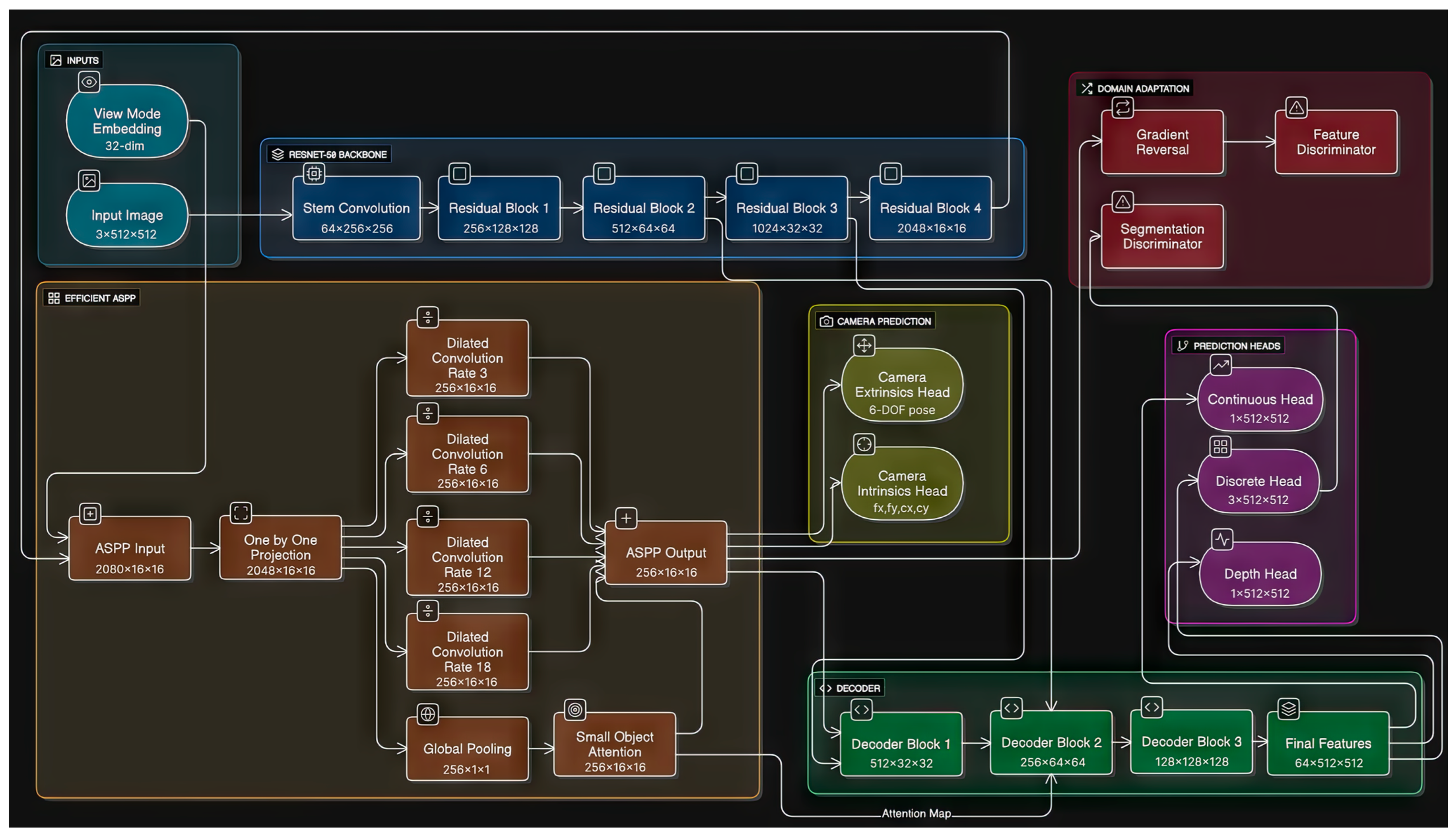
4.3. Custom DeeplabV3+ Architecture

Figure 5 illustrates the block diagram of the second stage model. The Multi-Task DeepLab architecture follows a hierarchical feature processing paradigm with four distinct transformation stages. A modified ResNet-50 backbone first extracts hierarchical features at progressively reduced spatial resolutions of 1/2, 1/4, 1/8, and 1/32 relative to the original input. This backbone serves as the foundation, where each downsampling stage strategically reduces spatial resolution while expanding channel capacity. A critical innovation occurs at the 1/32 scale feature level, where a 32-dimensional view embedding is injected through concatenation before ASPP processing. This view embedding encodes camera perspective information, such as ground-level or aerial views, allowing the network to adapt its receptive field characteristics based on the imaging perspective. The combined tensor then passes through a projection layer before entering the EfficientASPP module, which outputs 256-channel features. These features serve a dual purpose: they are utilized for camera parameter prediction and also as the primary input for the decoder pathway. The decoder progressively upsamples features through three Lightweight Decoder Blocks. These blocks transition the feature channel dimensions from 512, to 256, and finally to 128 channels. Each decoder block is a key innovation, meticulously incorporating skip connections from corresponding encoder stages and integrating Small-Object Attention (SOA) modules for refined feature fusion and enhancement of fine-grained details. The final shared features, refined to 64 channels, then feed into three parallel task-specific heads: a classifier for discrete-defect categorization across three predefined classes (e.g., crack, pothole, patch), a regressor for continuous severity estimation (e.g., defect intensity or area), and a depth predictor, providing a monocular depth map. Simultaneously, the camera predictor branch, operating directly from the ASPP features, outputs a 3 × 3 intrinsic matrix and a 3 × 4 extrinsic matrix, enabling geometric scene understanding. This architectural design with attention-guided skip connections and multi-task heads on a shared feature base ensures optimal activation distributions for each output type while minimizing parameter overhead.

4.3.1. Depthwise Separable Convolution (DSC)

To maintain real-time performance without sacrificing accuracy, the model systematically replaces standard convolutional layers with Depthwise Separable Convolutions (DSC). Each DSC operation decomposes a standard K × K convolution into two distinct computational stages: a depthwise convolution and a pointwise convolution. For an input tensor $X\in {\mathbb{R}}^{B\times C_{\mathrm{i}\mathrm{n}}\times H\times W}$, the depthwise convolution operates by applying a single 3 × 3 kernel to each input channel independently, with a stride of 1 and padding of 1. This step effectively learns spatial features for each channel without mixing information between channels. The output of the depthwise convolution, $Y=\mathrm{D}\mathrm{W}\mathrm{C}\mathrm{o}\mathrm{n}\mathrm{v}\left(X\right)$, is given by

$$Y_{\left(b,c,i,j\right)}={\sum }_{k_1=-1}^1{\sum }_{k_2=-1}^1{w}_{\left(c,k_1,k_2\right)}^d\cdot X_{\left(b,c,i+k_1,j+k_2\right)}$$

(7)

Following this, the pointwise convolution employs 1 × 1 kernels to linearly combine the outputs of the depthwise convolution across the channel dimension. This step maps the $C_{in}$ channels to $C_{out}$ channels, effectively mixing channel information. The output of the pointwise convolution, $Z=\mathrm{P}\mathrm{W}\mathrm{C}\mathrm{o}\mathrm{n}\mathrm{v}\left(Y\right)$, is:

$$Z_{\left(b,c^{\prime },i,j\right)}={\sum }_{c=1}^{C_{\mathrm{i}\mathrm{n}}}{w}_{\left(c^{\prime },c\right)}^p\cdot Y_{\left(b,c,i,j\right)}$$

(8)

This factorization yields significant parameter reduction. For a standard 3 × 3 convolution transforming $C_{in}$ channels to $C_{out}$ channels, the number of parameters is

$${\mathrm{P}\mathrm{a}\mathrm{r}\mathrm{a}\mathrm{m}\mathrm{s}}_{\mathrm{s}\mathrm{t}\mathrm{d}}=3^2\times C_{\mathrm{i}\mathrm{n}}\times C_{\mathrm{o}\mathrm{u}\mathrm{t}}$$

(9)

In contrast, for a depthwise separable convolution, the parameters are

$${\mathrm{P}\mathrm{a}\mathrm{r}\mathrm{a}\mathrm{m}\mathrm{s}}_{\mathrm{D}\mathrm{S}\mathrm{C}}=3^2\times C_{\mathrm{i}\mathrm{n}}+C_{\mathrm{i}\mathrm{n}}\times C_{\mathrm{o}\mathrm{u}\mathrm{t}}$$

(10)

This achieves an 8–9x parameter reduction compared to standard convolutions, particularly significant when processing high-channel features (e.g., 256 channels). Each DSC is consistently accompanied by batch normalization and ReLU activation. This optimization is systematically applied to all decoder blocks and ASPP modules, accounting for 72% of convolutional layers while utilizing only 18% of the total model parameters, thus enhancing efficiency without compromising representational capacity.

4.3.2. Small-Object Attention (SOA)

The Small-Object Attention (SOA) mechanism is a fundamental innovation addressing a critical challenge in road monitoring: the reliable detection and segmentation of sub-30px defects amidst complex pavement textures. The SOA module enhances small-defect detection through three coordinated pathways processing input features $X\in {\mathbb{R}}^{B\times C\times H\times W}$. The channel attention pathway computes channel-wise weights $w_c\in {\mathbb{R}}^C$ by first applying global average pooling to the input features. The resulting global descriptor is then processed by two 1 × 1 convolutional layers: the first reduces dimensionality to $\mathrm{C}/4$ channels, and the second expands it back to $C$ channels. a ReLU activation $\left(\delta \right)$ is applied between these convolutions, and a Sigmoid activation $\left(\sigma \right)$ provides the final gating weights:

$$w_c=\sigma \left(W_2\left(\delta \left(W_1\left(GAP\left(X\right)\right)\right)\right)\right)$$

(11)

The multi-scale spatial attention pathway focuses on spatial context at multiple scales. It begins by computing the channel-wise mean of the input features, $\overline{X}\in {\mathbb{R}}^{B\times 1\times H\times W}: \overline{X}={\displaystyle \frac{1}{C}}\sum _{c=1}^C{X}_c$. This mean-reduced feature is then passed through a shared 3 × 3 convolution. To capture multi-scale information efficiently, average pooling operations with varying kernel sizes $k\in \{1,3,5,7\}$ (with stride 1 and padding $k//2$) are applied. The outputs from these four pooling operations $\left(f_k\right)$ are concatenated along the channel dimension (yielding 16 channels). Finally, a 1 × 1 convolution projects this concatenated tensor to spatial weights $w_s\in {\mathbb{R}}^{1\times H\times W}$ via a Sigmoid activation:

$$w_s=\sigma \left({Conv}_{1\times 1}\left(Concat\left(f_1,f_3,f_5,f_7\right)\right)\right)$$

(12)

Complementing these, the small-object detector pathway acts as a lightweight high-pass filter, amplifying local intensity variations characteristic of cracks and potholes. It applies a 3 × 3 average pooling operation followed by a 1 × 1 convolution to generate small-object-specific weights $w_o\in {\mathbb{R}}^{1\times H\times W}$, also with a Sigmoid activation:

$$w_o=\sigma \left({Conv}_{1\times 1}\left({AvgPool}_{3\times 3}\left(X\right)\right)\right)$$

(13)

The final output of the SOA module combines these attention mechanisms multiplicatively with the original features.

$$\mathrm{S}\mathrm{O}\mathrm{A}\left(X\right)=X\odot \left(1+w_s+\alpha w_o\right)\odot w_c$$

(14)

where ⊙ denotes element-wise multiplication, and $\alpha =0.3$ is a weighting factor. This factor is crucial for balancing spatial enhancement against potential noise amplification, preventing over-emphasis on tiny artifacts that could represent imaging noise rather than true defects. This refined attention mechanism significantly enhances small-defect detection, leading to improvements such as a 12.7% increase in mAP for sub-32px defects, while adding only 0.4 million parameters per instantiation, demonstrating an excellent trade-off between performance gain and computational cost.

4.3.3. Efficient Atrous Spatial Pyramid Pooling (E-ASPP)

The Efficient ASPP module extends standard atrous convolution approaches by incorporating defect-scale-specific dilation rates and a key innovation: the integration of SOA processing within its global context branch. This allows the network to selectively emphasize small-defect-relevant features during context aggregation. The E-ASPP module processes 2048-channel inputs through four parallel branches featuring dilated DSC. The dilation rates (rates = [3, 6, 12, 18]) are specifically tuned to road defect scales, allowing the module to capture context at increasingly larger effective receptive fields while preserving fine details relevant to small defects. Each branch implements a DSC with a kernel size of 3, padding equal to its dilation rate, and the corresponding dilation. This is followed by and ReLU activation. Formally, for each rate $r\in \left\{3,6,12,18\right\}$, a feature map $F_r$ is computed:

$$F_r=\mathrm{R}\mathrm{e}\mathrm{L}\mathrm{U}\left(BN\left({DSC}_{3\times 3}\left(X;dilation=r\right)\right)\right)$$

(15)

A fifth global context path supplements these parallel branches. This path captures scene-level information by first applying adaptive average pooling to the input features. The pooled features are then transformed by a 1 × 1 convolution and ReLU activation. Crucially, the output of this convolution is then enhanced by a Small-Object Attention module:

$$G=\mathrm{S}\mathrm{O}\mathrm{A}\left(ReLU\left({Conv}_{1\times 1}\left(GAP\left(X\right)\right)\right)\right)$$

(16)

The resulting global feature $G$ is then bilinearly upsampled to match the spatial dimensions of the dilated convolutional outputs. The outputs from all five pathways (the four dilated branches and the upsampled global context branch) are concatenated along the channel dimension. This concatenated tensor then undergoes projection through a final DSC with a 1 × 1 kernel, reducing the dimensionality to 256 channels, accompanied by batch normalization, ReLU activation, and dropout. The overall E-ASPP output is

$$\mathrm{E}-\mathrm{A}\mathrm{S}\mathrm{P}\mathrm{P}\left(X\right)=\mathrm{R}\mathrm{e}\mathrm{L}\mathrm{U}\left(BN\left({DSC}_{1\times 1}\left(Concat\left(F_3,F_6,F_{12},F_{18},G^{\uparrow }\right)\right)\right)\right)$$

(17)

where $G^{\uparrow }$ denotes the upsampled global feature. This optimized design captures multi-scale context with only 2.1 million parameters—less than half of the 4.8 million parameters in standard ASPP implementations—while maintaining an expansive 968 × 968 pixel effective receptive field at the 1/32 feature scale, which is crucial for contextual understanding of distributed road defects.

4.3.4. Lightweight Decoder

Each Lightweight Decoder Block employs a consistent sequence of operations to upsample input features $x\in {\mathbb{R}}^{B\times C_1\times H\times W}$ and fuse them with higher-resolution skip connections $s\in {\mathbb{R}}^{B\times C_2\times H^{\prime }\times W^{\prime }}$. The process begins with bilinear interpolation to dynamically match the spatial dimensions of the input features $x$ to those of the higher-resolution skip connection $s$.

$$x_{\mathrm{u}\mathrm{p}}=\mathrm{BilinearUpsample}\left(x,\mathit{scale} \mathit{factor}={\displaystyle \frac{H_{skip}}{H_x}}\right)$$

(18)

The upsampled features $x_{\mathrm{u}\mathrm{p}}$ are then concatenated with the skip connection s along the channel dimension:

$$x_{\mathrm{c}\mathrm{a}\mathrm{t}}=\mathrm{C}\mathrm{o}\mathrm{n}\mathrm{c}\mathrm{a}\mathrm{t}\left(x_{up},s\right)$$

(19)

The fused features then pass through a depthwise convolution with a kernel size of 3 and padding of 1, reducing the dimensionality to the specified output channels $C_{\mathrm{o}\mathrm{u}\mathrm{t}}$. This is followed by batch normalization, ReLU activation, and crucially, SOA refinement:

$$x_{\mathrm{o}\mathrm{u}\mathrm{t}}=\mathrm{S}\mathrm{O}\mathrm{A}\left(ReLU\left(BN\left({DSC}_{3\times 3}\left(x_{cat}\right)\right)\right)\right)$$

(20)

The three decoder blocks progressively increase spatial resolution while managing channel dimensions. The first block combines 256-channel inputs from ASPP with 1024-channel skip features from the third encoder block to produce 512-channel outputs. The second block processes 512-channel inputs from first block with 512-channel skips from the second encoder block to yield 256 channels. The final block fuses 256-channel inputs from second block with 256-channel skips from first encoder block to generate 128-channel features. This hierarchical recovery of spatial details maintains computational efficiency through extensive use of depthwise separable convolutions, requiring only 3.2 million parameters across all decoder stages.

4.3.5. Camera Parameter Predictor

The Camera Parameter Predictor embodies a novel self-supervised approach to geometric scene understanding. By estimating both intrinsic and extrinsic parameters directly from visual features, the system eliminates the need for physical calibration targets while maintaining metric accuracy. The physics-informed initialization serves two purposes: it provides reasonable starting values for focal lengths and principal points, and it prevents early training instability that could propagate to other tasks. The camera prediction module estimates intrinsic and extrinsic parameters directly from the 256-channel ASPP features. Global average pooling first condenses spatial information into a 256-dimensional feature vector $f$, which feeds into two parallel fully connected branches.

The intrinsic prediction branch consists of two linear layers (256 → 128 → 4) outputting raw values for focal lengths $(v_{fx},v_{fy})$ and principal point coordinates $(v_{cx},v_{cy})$, contained in a vector ${\mathrm{v}}_{int}:$

$${\mathrm{v}}_{int}=[v_{fx},v_{fy},v_{cx},v_{cy}]={\mathrm{F}\mathrm{C}}_{int}\left(\mathrm{f}\right)$$

(21)

Physics-informed initialization sets initial biases to approximate common values for road monitoring cameras. To ensure positive focal lengths, $v_{fx} \mathrm{and} v_{fy}$ are activated via a softplus function, which serves as a smooth approximation of the ReLU function, and offset by a small epsilon (10⁻⁵):

$$F_{\mathrm{s}\mathrm{h}\mathrm{a}\mathrm{r}\mathrm{e}\mathrm{d}}=\mathrm{R}\mathrm{e}\mathrm{L}\mathrm{U}\left(BN\left({DSC}_{3\times 3}\left(F_{final features}\right)\right)\right)$$

(22)

Physics-informed initialization sets initial biases to approximate common values for road monitoring cameras. To ensure positive focal lengths, $v_{fx} \mathrm{a}\mathrm{n}\mathrm{d} v_{fy}$ are activated via a softplus function, which serves as a smooth approximation of the ReLU function, and offset by a small epsilon $\left({10}^{-5}\right):$

$$f_x=\mathrm{s}\mathrm{o}\mathrm{f}\mathrm{t}\mathrm{p}\mathrm{l}\mathrm{u}\mathrm{s}\left(v_{fx}\right)+ϵ,f_y=\mathrm{s}\mathrm{o}\mathrm{f}\mathrm{t}\mathrm{p}\mathrm{l}\mathrm{u}\mathrm{s}\left(v_{fy}\right)+ϵ$$

(23)

These parameters, along with the direct outputs $c_x=v_{cx} \mathrm{and} c_y=v_{cy},$ form the 3 × 3 intrinsic matrix $K$:

$$K=\left[\begin{array}{ccc}{f}_x& 0& c_x\\ 0& f_y& c_y\\ 0& 0& 1\end{array}\right]$$

(24)

The extrinsic branch employs two linear layers (256 → 128 → 6) predicting three rotation parameters (as an axis-angle vector $\omega$) and three translation components $t$:

$$[\omega ,\mathbf{t}]={\mathrm{F}\mathrm{C}}_{ext}\left(\mathbf{f}\right)$$

(25)

The rotation parameters ω are converted to a 3 × 3 rotation matrix $R$ via Rodrigues’ formula. First, the rotation magnitude $\left(angle\right)\theta =\left|\left|\omega \right|\right|$ and the unit rotation axis $a=\omega /\theta$ are computed. The skew-symmetric cross-product matrix $[a]\times$ is constructed from $\mathrm{a}=[a_x,a_y,a_z{]}^T:$

$${\left[\mathbf{a}\right]}_{\times }=\left[\begin{array}{ccc}0& -a_z& a_y\\ a_z& 0& -a_x\\ -a_y& a_x& 0\end{array}\right]$$

(26)

Then, the rotation matrix R is given by

$$R=I+\left(\mathrm{s}\mathrm{i}\mathrm{n}\theta \right)[\mathbf{a}{]}_{\times }+(1-\mathrm{c}\mathrm{o}\mathrm{s}\theta \left)\right[\mathbf{a}{]}_{\times }^2$$

(27)

where $I$ is the 3 × 3 identity matrix. The final extrinsic matrix, representing the world-to-camera transformation, is constructed as $T_{w\to c}=\left[R\right|\mathbf{t}]$. These predicted parameters are crucial for enabling 3D reconstruction through back-projection of predicted depth values $D(u,v).$

4.3.6. Multi-Task Prediction Heads

The Multi-Task DeepLab employs a shared-feature, specialized-head design, reflecting an optimal balance between task synergy and output-specific processing. All prediction tasks share a common 64-channel feature base, which is processed through a depthwise separable convolution, batch normalization, and ReLU activation, ensuring consistent feature normalization across tasks.

$$F_{\mathrm{s}\mathrm{h}\mathrm{a}\mathrm{r}\mathrm{e}\mathrm{d}}=\mathrm{R}\mathrm{e}\mathrm{L}\mathrm{U}\left(BN\left({DSC}_{3\times 3}\left(F_{final features}\right)\right)\right)$$

(28)

where $F_{\mathrm{final} \mathrm{features}}$ are the output features after the decoder. Task-specific heads then diverge: the discrete-defect classification head applies a 1 × 1 convolution to number of discrete classes (3) output channels. A softmax activation is typically applied during loss calculation for classification.

$$Y_{\mathrm{d}\mathrm{i}\mathrm{s}\mathrm{c}\mathrm{r}\mathrm{e}\mathrm{t}\mathrm{e}}={\mathrm{C}\mathrm{o}\mathrm{n}\mathrm{v}}_{1\times 1}\left(F_{shared}\right)$$

(29)

The continuous severity estimation head uses a 1 × 1 convolution to a single channel with Sigmoid activation. The sigmoid bounds the output to [0, 1], which can then be scaled to physical units based on calibration data:

$$Y_{\mathrm{continuous}}=\sigma \left({Conv}_{1\times 1}\left(F_{shared}\right)\right)$$

(30)

The depth prediction head employs a 1 × 1 convolution to one channel, also with Sigmoid activation, mapping depth values to a normalized range:

$$Y_{\mathrm{d}\mathrm{e}\mathrm{p}\mathrm{t}\mathrm{h}}=\sigma \left({Conv}_{1\times 1}\left(F_{shared}\right)\right)$$

(31)

This shared-representation approach enables joint optimization of complementary tasks while maintaining head efficiency at only 4.8 thousand combined parameters, demonstrating efficient multi-task learning.

4.3.7. View Adaptation

The view embedding system provides a lightweight yet effective mechanism for perspective adaptation. A compact learnable embedding table—view embedding—provides perspective-specific conditioning. The view identifier (0 for ground-level, 1 for aerial perspectives) indexes this table to retrieve a 32-dimensional vector:

$$e_{\mathrm{v}\mathrm{i}\mathrm{e}\mathrm{w}}=\mathrm{Embedding}(\mathrm{view} \mathrm{id})\in {\mathbb{R}}^{32}$$

(32)

During concatenation, these embeddings are spatially replicated to match the spatial dimensions of the deepest backbone features $(H/32, W/32):$

$$E_{\mathrm{s}\mathrm{p}\mathrm{a}\mathrm{t}\mathrm{i}\mathrm{a}\mathrm{l}}=e_{\mathrm{v}\mathrm{i}\mathrm{e}\mathrm{w}}.\mathrm{v}\mathrm{i}\mathrm{e}\mathrm{w}\left(B,embeddim,1,1\right).\mathrm{e}\mathrm{x}\mathrm{p}\mathrm{a}\mathrm{n}\mathrm{d}\left(-1,-1,{\displaystyle \frac{H}{32}},{\displaystyle \frac{W}{32}}\right)$$

(33)

This spatially replicated embedding is then concatenated to the backbone features (e4) before ASPP processing. The input to the ASPP module $\left(x_{asppinput}\right)$ is formed by a 1 × 1 convolution on this concatenated tensor:

$$x_{\mathrm{asppinput}}={\mathrm{C}\mathrm{o}\mathrm{n}\mathrm{v}}_{1\times 1}\left(Concat\left(e4,E_{spatial}\right)\right)$$

(34)

This approach is more parameter-efficient than alternative conditioning methods, such as branching entire network pathways, allowing the model to adapt feature processing to different camera geometries while sharing the majority of parameters across viewing perspectives. The 32-dimensional embedding space was found sufficient to encode the continuum between ground-level and aerial perspectives through linear interpolation.

4.3.8. Domain Adaptation

For unsupervised domain adaptation scenarios, the architecture incorporates a Domain Adapter module, which leverages three synergistic components operating at different feature levels. This integrated approach, adding only 0.9 million parameters, significantly improves cross-domain generalization, as measured by performance on unseen geographical regions and imaging conditions. The complete adaptation framework operates through a minimax optimization: the feature extractor learns to fool both discriminators, while the discriminators improve at detecting domain origins. The semantic consistency loss anchors the representation to preserve defect semantics during adaptation.

The feature-level discriminator $\left(D_{\mathrm{f}\mathrm{e}\mathrm{a}\mathrm{t}}\right)$ analyzes the ASPP output features $\left(F_{ASPP}\right)$ to align intermediate representations between source and target domains. Its architecture employs progressively strided convolutions to build domain-invariant features. Crucially, a Gradient Reversal Layer (GRL) is placed before its final linear layer, ensuring adversarial training dynamics. The GRL Gradient Reversal function reverses the gradient sign during backpropagation

$${\displaystyle \frac{\mathsf{\partial }{L}_{\mathrm{a}\mathrm{d}\mathrm{v}}}{\mathsf{\partial }{F}_{\mathrm{A}\mathrm{S}\mathrm{P}\mathrm{P}}}}=-\lambda {\displaystyle \frac{\mathsf{\partial }{L}_{\mathrm{d}\mathrm{o}\mathrm{m}\mathrm{a}\mathrm{i}\mathrm{n}}}{\mathsf{\partial }{F}_{\mathrm{A}\mathrm{S}\mathrm{P}\mathrm{P}}}}$$

(35)

where $\lambda$ is the weight factor. The discriminator then classifies the domain origin. The code implements a simpler 2D convolution (256, 64, 3) followed by Gradient Reversal Layer (GRL) and then adaptive average pooling and a linear layer (64, 1). The output-level discriminator $\left(D_{\mathrm{s}\mathrm{e}\mathrm{g}}\right)$ (self.seg_discriminator) operates on the semantic segmentation logits (Y_seg, from outputs[‘discrete’]) to enforce task-consistent domain alignment. It has a similar structure, also incorporating a GRL. The code implements a convolution with shape (num_classes, 64, 3) followed by GRL and then average pool and linear (64, 1). An auxiliary segmentation head provides additional regularization by maintaining semantic consistency regardless of domain shifts. It is implemented as a 1 × 1 convolution with shape (256, num_classes, 1) on the ASPP features $\left(F_{ASPP}\right)$. The consistency loss $\left(L_{cons}\right)$ then ensures that the auxiliary predictions align with ground truth or pseudo-labels, especially in unsupervised settings

$$L_{\mathrm{c}\mathrm{o}\mathrm{n}\mathrm{s}}=-{\sum }_{c=1}^{\mathrm{num} \mathrm{classes}}{y}_c\mathrm{l}\mathrm{o}\mathrm{g}\left(\mathrm{s}\mathrm{o}\mathrm{f}\mathrm{t}\mathrm{m}\mathrm{a}\mathrm{x}\right(W_{\mathrm{a}\mathrm{u}\mathrm{x}}{F}_{\mathrm{A}\mathrm{S}\mathrm{P}\mathrm{P}}{)}_c)$$

(36)

where $y_c$ are the ground truth (or pseudo) labels and $W_{\mathrm{a}\mathrm{u}\mathrm{x}}$ are the weights of the auxiliary 1 × 1 convolution. The complete system implements the following adversarial loss formulation for domain adaptation, where the discriminators aim to minimize this loss, while the feature extractor and generator implicitly maximize it due to the GRL

$$L_{\mathrm{a}\mathrm{d}\mathrm{v}}={\mathbb{E}}_{x_s\sim p_s}\left[\mathit{log}D\left(F\left(x_s\right)\right)\right]+{\mathbb{E}}_{x_t\sim p_t}\left[\mathit{log}\left(1-D\left(F\left(x_t\right)\right)\right)\right]$$

(37)

where $x_s$ and $x_t$ represent source and target domain inputs, respectively, $D$ is the discriminator, and $F$ represents the features being discriminated. This integrated approach allows the model to learn features that are simultaneously discriminative for the main tasks and invariant to domain shifts. The complete architecture thus balances representational capacity and computational efficiency, with all components specifically optimized for real-time road monitoring requirements.

5. Experiments and Results

5.1. Training Details

Our proposed framework is trained in a two-stage process. The first stage addresses pixel-level domain shift via image-to-image translation, while the second stage trains the main perception model. To enhance the realism of our synthetic data, we first train a modified CycleGAN model with a nine-block ResNet generator. This model learns an unpaired translation from our synthetic images to the style of real-world datasets. Training is conducted for 200 epochs: 100 at a stable learning rate of $2\times {10}^{-4}$, followed by 100 with the learning rate linearly decaying to zero. We use the Adam optimizer $({\beta }_1=0.5)$ and stabilize adversarial training with the Least Squares GAN (LSGAN) loss. The loss function includes a cycle-consistency term $(\lambda =10)$, an identity loss $(\lambda =0.5),$ and our novel defect-preserving loss $\left({\lambda }_{defect}=5.0\right)$ to ensure semantic fidelity during translation. Next is the multi-task and adversarial model training. For the main training, our core perception model, a Multi-Task DeepLab architecture, is encapsulated within a Domain Adapter wrapper. This wrapper model facilitates our domain adaptation strategy by integrating dedicated discriminator networks. The complete system is trained for 200 epochs using the Adam optimizer $\left({\beta }_1=0.9, {\beta }_2=0.999\right)$ with an initial learning rate of $1\times {10}^{-4}$. The learning rate is managed by a reduce learning rate on plateau scheduler, which reduces the learning rate if the validation loss plateaus. To ensure training stability, we employ gradient clipping with a maximum norm of 1.0 and utilize automatic mixed precision (AMP). The total loss ${\mathcal{L}}_{\mathrm{t}\mathrm{o}\mathrm{t}\mathrm{a}\mathrm{l}}$ is a weighted summation of the main supervised task loss $\left({\mathcal{L}}_{task}\right)$, two adversarial losses $\left({\mathcal{L}}_{adv}\right)$, and a view-consistency loss $\left({\mathcal{L}}_{\mathrm{v}\mathrm{i}\mathrm{e}\mathrm{w}}\right).$

$${\mathcal{L}}_{\mathrm{t}\mathrm{o}\mathrm{t}\mathrm{a}\mathrm{l}}=w_{\mathrm{t}\mathrm{a}\mathrm{s}\mathrm{k}}{\mathcal{L}}_{\mathrm{t}\mathrm{a}\mathrm{s}\mathrm{k}}+{\lambda }_{{\mathrm{a}\mathrm{d}\mathrm{v}}_{\mathrm{f}\mathrm{e}\mathrm{a}\mathrm{t}}}{\mathcal{L}}_{{\mathrm{a}\mathrm{d}\mathrm{v}}_{\mathrm{f}\mathrm{e}\mathrm{a}\mathrm{t}}}+{\lambda }_{{\mathrm{a}\mathrm{d}\mathrm{v}}_{\mathrm{s}\mathrm{e}\mathrm{g}}}{\mathcal{L}}_{{\mathrm{a}\mathrm{d}\mathrm{v}}_{\mathrm{s}\mathrm{e}\mathrm{g}}}+{\lambda }_{\mathrm{v}\mathrm{i}\mathrm{e}\mathrm{w}}{\mathcal{L}}_{\mathrm{v}\mathrm{i}\mathrm{e}\mathrm{w}}$$

(38)

The main task loss, ${\mathcal{L}}_{\mathrm{task}}$, is itself a weighted sum of segmentation, depth, and camera losses

$${\mathcal{L}}_{\mathrm{t}\mathrm{a}\mathrm{s}\mathrm{k}}=w_{\mathrm{s}\mathrm{e}\mathrm{g}}{\mathcal{L}}_{\mathrm{s}\mathrm{e}\mathrm{g}}+w_{\mathrm{d}\mathrm{e}\mathrm{p}\mathrm{t}\mathrm{h}}{\mathcal{L}}_{\mathrm{d}\mathrm{e}\mathrm{p}\mathrm{t}\mathrm{h}}+w_{\mathrm{c}\mathrm{a}\mathrm{m}}{\mathcal{L}}_{\mathrm{c}\mathrm{a}\mathrm{m}}$$

(39)

with weights $w_{\mathrm{seg}},w_{\mathrm{depth}},$ and $w_{\mathrm{cam}}$ set to 1.5, 1.0, and 0.3, respectively. Each component is defined as follows:

Segmentation Loss $\left({\mathcal{L}}_{seg}\right):$ This loss handles both discrete and continuous defects. For discrete classes (crack, manhole, patch), we use a weighted Binary Cross-Entropy (BCE) loss on the road area with pos_weight values of [5.0, 10.0, 8.0] to counteract class imbalance. To suppress false positives in non-road areas, we apply a separate, per-channel weighted BCE loss with higher penalties for classes prone to errors. For the continuous pothole class, we use a robust L1 loss. Depth Loss $\left({\mathcal{L}}_{depth}\right)$: Depth estimation is supervised using a scale-invariant logarithmic error, which is robust to variations in absolute depth scale. The loss is computed as

$$\sqrt{\mathrm{V}\mathrm{a}\mathrm{r}(\Delta )+0.5\cdot \left(\mathrm{M}\mathrm{e}\mathrm{a}\mathrm{n}\right(\Delta ){)}^2},\mathrm{w}\mathrm{h}\mathrm{e}\mathrm{r}\mathrm{e}\mathrm{ }\Delta =\mathrm{l}\mathrm{o}\mathrm{g}\left({\widehat{y}}_{\mathrm{d}\mathrm{e}\mathrm{p}\mathrm{t}\mathrm{h}}\right)-\mathrm{l}\mathrm{o}\mathrm{g}\left(y_{\mathrm{d}\mathrm{e}\mathrm{p}\mathrm{t}\mathrm{h}}\right)$$

(40)

Camera Parameter Loss $\left({\mathcal{L}}_{cam}\right)$: To ensure geometric realism, the camera loss enforces multiple constraints. It combines an L1 loss on the intrinsic parameters with a composite loss on the predicted rotation matrix $\widehat{R}.$ This rotation loss includes a direct MSE term against the ground truth, an orthogonality constraint $\left(\right||\widehat{R}{\widehat{R}}^{\mathrm{\top }}-\mathbf{I}|{|}_2),$ and a determinant constraint $(\parallel det(\widehat{R})-1{\parallel }_2)$ to ensure $\widehat{R}$ is a valid rotation matrix. A scale-invariant L1 loss is used for the translation vector.

Adversarial and Consistency Losses: To align the synthetic and real domains, we use two adversarial losses on the feature and segmentation outputs, weighted by ${\lambda }_{{\mathrm{adv}}_{\mathrm{feat}}}=0.1$ and ${\lambda }_{{\mathrm{adv}}_{\mathrm{seg}}}=0.1$. The discriminators are trained to distinguish between synthetic and real data, while a GRL trains the main model to produce domain-agnostic outputs. A view-consistency loss $\left({\mathcal{L}}_{view}\right)$, weighted by ${\lambda }_{\mathrm{v}\mathrm{i}\mathrm{e}\mathrm{w}}=0.1$, encourages the feature extractor to produce similar representations for the same scene from both dashcam and drone perspectives.

5.2. Qualitative Analysis

5.2.1. Image Translation Predictions

This subsection presents the qualitative results for our first-stage model, the segmentation-aware CycleGAN, which is responsible for image-to-image translation from Domain A (original road images) to Domain B (translated/normalized road images). The primary objective of this stage is to generate synthetic images that normalize visual variations in the input data while preserving critical information about road defects, thus providing a consistent and robust input for the subsequent road defect prediction stage.

Figure 6 illustrates a series of representative examples showcasing the performance of the trained CycleGAN for the dashcam view. Our CycleGAN generated the corresponding output. Observe how the model successfully transforms the visual style of the original image to the target domain. This translation typically involves normalization of brightness, contrast, and color balance, aiming for a more uniform appearance across different scenes. The top row shows the synthetic images with the background replaced with the real domain data so that the style translation process will be more straightforward compared to a noisy black background. This process allows visual artifacts and noise from the original image to be suppressed, and the background elements not relevant to the road surface (e.g., surrounding environment, sky) are often rendered with a consistent, simplified style. We found this to be better than having an empty background in the fake domain images.

Similarly, Figure 7 illustrates some of the translation predictions for the drone view dataset. CycleGAN demonstrates a strong ability to generalize across diverse input images from Domain A. The generated images in Domain B exhibit a consistent visual style, which is less susceptible to variations in ambient lighting or distracting background elements present in the original capture. This uniform representation is expected to enhance the robustness and accuracy of the subsequent DeepLabv3+ model by providing it with a more standardized visual input, thereby reducing the impact of irrelevant domain shifts. The careful preservation of defect features across the translation is a key achievement, ensuring that the critical information for road defect prediction is not lost during this pre-processing stage.

5.2.2. Road Defect Predictions

This section details the performance of our Modified DeepLabv3+ model in predicting road defects. The model takes either the CycleGAN-translated images (during evaluation after Stage 1 processing) or raw road images (for direct inference) as input and performs multi-task prediction, including discrete-defect segmentation, continuous defect intensity estimation, and depth mapping. Figure 8 provides a qualitative overview of the model’s prediction capabilities across diverse road scenarios. Figure 8a–d represent the input image fed into the DeepLabv3+ model. Depending on your experimental setup, this could be an original road image or a CycleGAN-translated image (e.g., “Generated Image B” from Stage 1). Highlighting whether these are raw or translated images is crucial for context. Figure 8e–h represent predicted defect masks from multiple heads combined. As shown in Figure 8, the model accurately delineates these defects, capturing their intricate shapes and locations. The thresholding value of 0.5 is applied to convert the raw probabilistic outputs into clear binary masks, facilitating visual interpretation. Beyond simple presence/absence, the model predicts continuous values for specific defect characteristics, such as ‘pothole’ or ‘puddle’ severity. This map, typically visualized as a grayscale or heatmap, provides a nuanced understanding of defect intensity or extent. For instance, brighter regions could indicate deeper potholes or larger puddles, offering richer information than a binary mask alone. Figure 8i–l represents the predicted depth map. This output provides per-pixel depth estimation for the scene. As illustrated, the depth map (often normalized for visualization) captures the three-dimensional structure of the road scene, showing variations in elevation that correspond to the objects in the scene. This geometric understanding can be invaluable for advanced road condition assessment, aiding in defect volumetric calculations.

Similarly, Figure 9 illustrates some of the translation predictions for the drone view dataset. Figure 9a–d represent the input image fed into the DeepLabv3+ model. Figure 9e–h represent predicted defect masks from multiple heads combined. Figure 9i–l represent predicted depth maps. The effectiveness of specialized components like Small-Object Attention, Efficient ASPP, and Lightweight Decoder Blocks is evident in the model’s ability to precisely identify both large and small-scale defects, often overlooked by traditional segmentation architectures. The integration of View Mode embedding further contributes to the model’s adaptability across varying perspectives of road capture. The results demonstrate that our Modified DeepLabv3+ model is not only capable of robustly segmenting multiple types of road defects but also provides complementary continuous and geometric information, offering a comprehensive understanding of road surface conditions. This multi-task approach contributes to a more holistic and actionable road inspection system.

To supplement our quantitative metrics, we conducted a qualitative analysis of the model’s performance on a diverse set of real-world dashcam images, as illustrated in Figure 10. Figure 10a–d illustrate some of the easy defect samples and their predictions. Figure 10e–h illustrate some of the hard defect samples which present more complex scenarios where the model continues to perform robustly, successfully identifying defects with less distinct boundaries or partial obstructions. Figure 10i–l illustrate some of the challenging defect samples and their predictions. Although our model is powerful in predicting a wide variety of cracks like longitudinal, transverse, and alligator cracks, many challenging scenarios are not being addressed while developing the dataset, such as mirror reflections and objects like car wiper which is visible in the dashcam footage and also environmental problems like shadows cast by trees and buildings. We observed that the presence of these artifacts and conditions is the primary cause of false-positive predictions in real-world testing. Addressing these specific environmental and hardware-related challenges represents a key direction for future work, potentially through targeted data augmentation or the inclusion of a dedicated module for artifact detection.

5.2.3. Three-Dimensional Reconstruction

To elevate the utility of our 2D predictions for practical asset management and quantitative analysis, we developed a pipeline to reconstruct the detected road defects in a 3D world space. This process transforms the sequential, per-frame outputs from our multi-task model into a cohesive 3D point cloud, which can then be visualized as a comprehensive top-down defect map. The methodology is divided into two primary stages: (1) per-frame 3D point generation and aggregation and (2) Bird’s-Eye View (BEV) map creation.

To provide a clear and measurable 2D overview of the reconstructed 3D scene, a Bird’s-Eye View (BEV) map is generated from the aggregated point cloud. The 3D point cloud is first filtered to isolate points lying on the road surface. This is achieved by applying a height threshold along the Y-axis (vertical), effectively removing points corresponding to vehicles, buildings, or noise. The filtered ground points are then orthographically projected onto a 2D grid. The world-space X and Z coordinates of each point are mapped to pixel coordinates in the BEV image. The color of each pixel in the BEV map is determined by the color of the 3D point that projects onto it. This process results in a high-resolution, top-down image that serves as a geospatial map of the surveyed area, clearly visualizing the location, shape, and classification of all detected road defects. This BEV map is invaluable for tasks such as calculating defect area, assessing spatial distribution, and planning maintenance activities.

For 3D point generation and aggregation, the first stage processes an input video stream frame-by-frame to generate a colored 3D point cloud. For each frame, the following steps are executed. The video frame is preprocessed and passed through our trained multi-task model to yield the predicted discrete segmentation map $\left(M_{seg}\right)$, continuous severity map $\left(M_{cont}\right)$, depth map $\left(D\right)$, intrinsic camera matrix $\left(K\right)$, and extrinsic camera matrix ${(T}_{c\to w})$. Each pixel $(u,v)$ in the 2D prediction maps is unprojected into a 3D point in the camera’s local coordinate system. Using the pinhole camera model, the 3D coordinates $\left(X_c,Y_c,Z_c\right)$ are calculated as follows.

$$Z_c=D\left(u,v\right)$$

(41)

$$X_c={\displaystyle \frac{(u-c_x)\cdot Z_c}{f_x}}$$

(42)

$$Y_c={\displaystyle \frac{(v-c_y)\cdot Z_c}{f_y}}$$

(43)

where $(f_x,f_y)$ are the focal lengths and $(c_x,c_y)$ are the principal point coordinates extracted from the predicted intrinsic matrix $K$. The points from the camera’s coordinate system are transformed into a global world coordinate system. This is achieved by applying the inverse of the predicted extrinsic matrix $\left(T_{w\to c}\right)$, which represents the camera-to-world transformation ${(T}_{c\to w}=T_{w\to c}^{-1}).$ Figure 11 illustrates the reconstruction results for a video frame data. Each generated 3D point is assigned a color based on its corresponding class in the discrete segmentation map $\left(M_{seg}\right).$ For instance, cracks are colored red, patches green, and non-defect road surfaces gray. These colored points from every frame are aggregated into a single, dense point cloud, effectively stitching together the predictions from the entire video sequence into one coherent 3D scene. The final aggregated point cloud is saved in the standard .ply format. Then the 3D point cloud is used to create a 2D bird’s-eye view for easier interpretation of results.

5.3. Quantitative Analysis

This section presents a comprehensive quantitative evaluation of our proposed two-stage model for road defect prediction. We assess both the individual contributions of each stage and the overall performance of the integrated system.

5.3.1. Stage 1: Segmentation-Aware CycleGAN Evaluation

The first stage of our model, the segmentation-aware CycleGAN, is crucial for image-to-image translation to normalize visual characteristics while preserving defect information. Its training dynamics are visually represented in Figure 12.

Figure 12 illustrates the evolution of various loss components during the training of our segmentation-aware CycleGAN. A key observation is the consistent and steady decrease in the cycle consistency losses $({\mathcal{L}}_{cycle\_A} \mathrm{a}\mathrm{n}\mathrm{d} {\mathcal{L}}_{cycle\_B})$ and the identity mapping losses $({\mathcal{L}}_{idt\_A} \mathrm{a}\mathrm{n}\mathrm{d} {\mathcal{L}}_{idt\_B})$ throughout training. The diminishing cycle loss signifies that the generators $\left(G_A \mathrm{a}\mathrm{n}\mathrm{d}{ G}_B\right)$ successfully learn nearly bijective mappings, allowing an image translated from one domain to another and back to be accurately reconstructed to its original form. Similarly, the converging identity losses confirm the generators’ ability to maintain inherent characteristics of an input image when it already belongs to the target domain, which is vital for preventing unwanted content distortions. Furthermore, our custom defect preservation loss $\left({\mathcal{L}}_{defect}\right)$ also shows a clear downward trend, validating its effectiveness in guiding the generator to maintain the integrity of road defect features during translation. These consistent decreases are crucial indicators of CycleGAN’s successful content-preserving image-to-image translation.

In contrast, the adversarial losses for both generators $({\mathcal{L}}_{G\_A},{\mathcal{L}}_{G\_B})$ and discriminators $({\mathcal{L}}_{D\_A},{\mathcal{L}}_{D\_B})$ present noticeable fluctuations, often resembling an ‘ECG signal’ pattern. This oscillatory behavior is characteristic and expected in GAN training, reflecting the dynamic minimax game between the generators and discriminators. As generators produce increasingly realistic images, they temporarily ‘win’ against their discriminators, forcing the discriminators to adapt and improve, thus perpetuating the competitive cycle. As long as these oscillations remain bounded and do not diverge, they indicate an active and ongoing learning process within the adversarial framework, essential for the generators to produce high-quality synthetic images. The combined behavior of these loss components, particularly the consistent convergence of the cycle consistency, identity, and defect preservation losses amidst the adversarial fluctuations, provides strong evidence for the robust learning of the CycleGAN. This stage effectively transforms input images while ensuring critical preservation of defect-related features, preparing the data for precise defect prediction by the subsequent DeepLabv3+ model.

5.3.2. Stage 2: Modified DeepLabv3+ Evaluation

Figure 13 illustrates the training dynamics of the Modified DeepLabv3+ model, showcasing the evolution of its multi-task loss components over epochs on the drone–dashcam dataset. The overall total training and validation losses generally exhibit a decreasing trend over epochs, indicating that the model is indeed learning from the provided data.

Upon closer examination of the individual loss components, it can be observed that the segmentation loss $\left({\mathcal{L}}_{Seg}\right)$ and the depth estimation loss $\left({\mathcal{L}}_{Depth}\right)$ both show consistent and healthy decreases, converging towards lower values. This confirms the model’s ability to learn pixel-wise defect masks and approximate depth values, fundamental to the proposed system. However, the camera parameter prediction loss $\left({\mathcal{L}}_{Cam}\right)$ stands out due to its significantly higher magnitude compared to the segmentation and depth losses. While it also shows a general decreasing trend, its scale (e.g., values ranging from ~78 down to ~75 in the initial epochs) is orders of magnitude larger. This disproportionate scale highlights the inherent challenge and potential sensitivity in accurately regressing complex Six-Degrees-of-Freedom (DoF) camera poses and intrinsic parameters from single images. The dominance of this loss component significantly influences the overall total loss, potentially masking the finer convergence dynamics of the segmentation and depth tasks. This behavior can be attributed to the intricate nature of geometric regression and the potential for noise or less precise ground truth data for camera parameters in real-world [drone/dashcam] datasets. The general convergence of the segmentation and depth losses suggests effective learning for these pixel-dense tasks. While the camera loss also decreases, its higher magnitude underscores the optimization challenges in multi-task learning when tasks differ vastly in scale and supervision quality. The relatively close proximity between the training and validation curves for individual components (especially segmentation and depth) indicates [acceptable generalization/no severe overfitting] for these specific tasks, further confirming the model’s ability to learn robust features for road defect analysis.

5.3.3. Computational Efficiency

Our proposed model was designed for both high accuracy and computational efficiency, making it suitable for real-time deployment in ADAS applications. The final model consists of 27.83 million trainable parameters. During inference on an NVIDIA V100 GPU with a 512 × 512 input image, the model achieves an average latency of 17.92 ms, which corresponds to a throughput of approximately 56 frames per second (FPS). This performance is largely attributed to the extensive use of depthwise separable convolutions in place of standard convolutions throughout the architecture, particularly within the E-ASPP and decoder blocks. This design choice significantly reduces the parameter count and computational load without compromising the model’s representational capacity.

5.3.4. Stage 2: Modified DeepLabv3+ Performance Metrics

The second stage, our Modified DeepLabv3+ model, performs multi-task road defect prediction. Its performance is evaluated through various quantitative metrics and training loss dynamics. The model’s performance for discrete road defect segmentation (crack, manhole, and patch), continuous defect severity prediction, and depth estimation was rigorously evaluated.

Table 1. Evaluation metrics of our model for road defect prediction.

Model	mIoU (%)	Precision (Avg)	Recall (Avg)	F1-Score (Avg)	MAE (Cont.)	RMSE (Depth)	Params (M)	Inference Time (ms)	FPS
DeepLabv3+	0.7521	0.8823	0.7975	0.8470	0.0057	0.0478	49.52	24.03	41.62
PSPNet	0.7652	0.8872	0.8206	0.8464	0.0066	0.0490	53.81	12.31	81.25
SegFormer-B0	0.5284	0.7890	0.6148	0.6886	0.0136	0.0908	5.11	16.66	60.02
Our Model	0.8021	0.9272	0.8520	0.8875	0.0055	0.0461	27.83	17.92	55.81

summarizes these results, including standard metrics such as Mean Intersection over Union (mIoU) for discrete predictions, Precision, Recall, and F1-score for segmentation, Mean Absolute Error (MAE) for continuous prediction, and Root Mean Squared Error (RMSE) for depth predictions.

We compare our proposed model against a baseline DeepLabv3+ and two other prominent SOTA architectures: PSPNet and SegFormer. Our proposed model achieves a state-of-the-art Mean Intersection over Union (mIoU) of 80.21%, outperforming all benchmarked architectures. This represents a significant 6.6% relative improvement in segmentation accuracy over the baseline DeepLabv3+ model, validating the superior design of our architectural enhancements, such as the Small-Object Attention and Efficient ASPP modules. In the auxiliary tasks, our model also demonstrates top-tier performance, recording the lowest Mean Absolute Error of 0.0055 for continuous defect severity and a Root Mean Squared Error of 0.0461 for depth estimation. Our model also surpasses other SOTA architectures, including PSPNet [12], which achieved a strong mIoU of 76.52%. While PSPNet’s pyramid pooling module is effective at capturing multi-scale context, our model’s tailored design proves more effective for the specific feature distribution within our drone dataset. Conversely, the SegFormer [30] model exhibited significantly lower performance, with an mIoU of only 52.84%. This result is not indicative of a flaw in the architecture itself but rather highlights a fundamental characteristic of Vision Transformers. Unlike CNNs, which possess a strong inductive bias for spatial locality, transformers must learn these relationships from scratch. Consequently, they require pre-training on massive datasets (e.g., ImageNet-22K) to be effective. As our experiment utilized a model without such large-scale pre-training, its performance was limited, underscoring the data efficiency of CNN-based approaches like ours for specialized tasks. The model comprises 56 M parameters, and the average inference time on an NVIDIA V100 GPU for a single 512 × 512 image is 17.92 ms (~56 FPS), confirming its suitability for practical deployment in road inspection systems.

To provide a more granular analysis of our model’s segmentation performance,

Table 2. Class-wise Intersection over Union (IoU) scores for discrete-defect types.

Model	mIoU (%)	Crack IoU (%)	Manhole IoU (%)	Patch IoU (%)
DeepLabv3+	0.7521	0.7878	0.7121	0.7563
PSPNet	0.7652	0.6704	0.7450	0.8802
SegFormer-B0	0.5284	0.4206	0.7500	0.4146
Our Model	0.8021	0.7141	0.7910	0.9579

presents the class-wise Intersection over Union (IoU) scores for the three discrete-defect categories. Our model demonstrates strong and balanced performance across all classes, achieving the highest IoU for cracks, manholes, and patches compared to the other benchmarked architectures. This indicates that our architectural enhancements, such as the Small-Object Attention (SOA) module, are particularly effective at distinguishing between different types of road features, even those that are small or visually subtle.

The predicted camera intrinsic and extrinsic parameters were evaluated against ground truth values.

Table 3. Camera parameter estimation accuracy.

Parameter	MAE (Mean Absolute Error)	RMSE (Root Mean Squared Error)
$f_x\left(\mathrm{p}\mathrm{i}\mathrm{x}\mathrm{e}\mathrm{l}\mathrm{s}\right)$	0.0028	0.0774
$f_y\left(\mathrm{p}\mathrm{i}\mathrm{x}\mathrm{e}\mathrm{l}\mathrm{s}\right)$	0.0065	0.1427
$c_x\left(\mathrm{p}\mathrm{i}\mathrm{x}\mathrm{e}\mathrm{l}\mathrm{s}\right)$	4.6634	4.6634
$c_y\left(\mathrm{p}\mathrm{i}\mathrm{x}\mathrm{e}\mathrm{l}\mathrm{s}\right)$	4.6634	4.6634
Rotation (degrees)	6.5439	16.1211
Translation (meters)	6.8563	14.7704

summarizes the accuracy of these estimations.

The intrinsic parameters $\left(f_x,f_y,c_x,c_y\right)$ showed a Mean Absolute Error of 0.0047 pixels for focal lengths and 4.66 pixels for principal points, respectively, indicating a high degree of accuracy in learning the camera’s internal properties. For extrinsic parameters, the mean angular error for rotation was 6.54 degrees, and the mean translation error was 6.86 m. While these results demonstrate the model’s ability to learn pose from a single image, the magnitude of the extrinsic errors highlights the inherent difficulty of achieving precise global localization, which explains the challenges in creating seamless 3D reconstruction.

5.4. Ablation Study

To rigorously evaluate the individual contributions of our proposed architectural and methodological components, we conducted a comprehensive ablation study for the dashcam view. The study was designed to systematically dissect the impact of three key innovations: (1) our custom-designed model architecture, (2) the two-stage sim-to-real domain adaptation, and (3) the specific benefit of our novel segmentation-aware loss within the CycleGAN framework. The study begins with a baseline model using a standard DeepLabV3+ architecture and progressively adds our contributions. For a fair and direct comparison, all models were trained on their respective datasets but evaluated on the exact same validation set, which was generated using our final segmentation-aware CycleGAN. The results are summarized in

Table 4. Ablation study results showing the impact of each component on segmentation performance (mIoU).

Step	Model Configuration	mIoU (%)
1	Baseline (Standard Architecture on Raw Synthetic Data)	0.6386
2	+Our Custom Architecture (on Raw Synthetic Data)	0.6969
3	+Standard CycleGAN Translation	0.7456
4	+Segmentation-Aware CycleGAN Translation	0.7749
5	+In-Training Adversarial Adaptation (Full Model)	0.8021

.

The results provide clear insights into the efficacy of each component. Step 1 establishes the performance of a standard architecture on the raw synthetic data. By introducing our custom architecture with SOA and E-ASPP modules (Step 2), the mIoU improved, demonstrating the effectiveness of our design in learning more robust features for road defect detection directly from the synthetic domain. The introduction of domain adaptation via a standard CycleGAN (Step 3) provided a significant performance boost, underscoring the critical need to bridge the synthetic-to-real domain gap. However, the most crucial finding is the comparison between Step 3 and Step 4. Replacing the standard CycleGAN with our proposed segmentation-aware CycleGAN yielded a substantial gain in mIoU. This validates our core hypothesis that preserving the geometric fidelity of small defects during image translation is paramount for achieving high performance. Finally, the inclusion of the in-training dual-discriminator adversarial learning (Step 5) pushed the performance to its peak. This confirms that our proposed two-stage domain adaptation strategy—a high-fidelity, content-aware pre-processing step followed by in-training feature alignment—is a highly effective approach that synergistically minimizes domain shift and maximizes segmentation accuracy.

5.5. Generalization on Real-World Data

To further validate the generalizability of our proposed sim-to-real framework, we performed an additional quantitative evaluation on a public, real-world benchmark. We used the Crack500 dataset, which consists of high-resolution images of actual pavement cracks with pixel-perfect ground-truth masks. Our fully trained model was evaluated on the official test set of this dataset without any fine-tuning. For this binary segmentation task, we used only the “cracks” output channel from our multi-task segmentation head. The results, presented in

Table 5. Quantitative results on the real-world Crack500 test set.

Model	IoU	Precision (Avg)	Recall (Avg)	F1-Score (Avg)
Our Model	0.7899	0.8850	0.8920	0.8885

, show that our model achieves strong performance on this unseen, real-world data. In addition to these metrics, Figure 14 provides a qualitative assessment of the model’s predictions on several examples from the test set. This successful transfer from our synthetic training environment to a challenging real-world benchmark validates the effectiveness of our two-stage domain adaptation strategy in bridging the sim-to-real gap and learning robust, generalizable features for road defect detection.

As illustrated in Figure 14, the model accurately delineates the intricate and fine-grained patterns of real-world cracks, often matching the ground-truth masks with high fidelity. This successful transfer, demonstrated both quantitatively and qualitatively, validates the effectiveness of our two-stage domain adaptation strategy in bridging the sim-to-real gap and learning robust, generalizable features for road defect detection.

6. Discussion

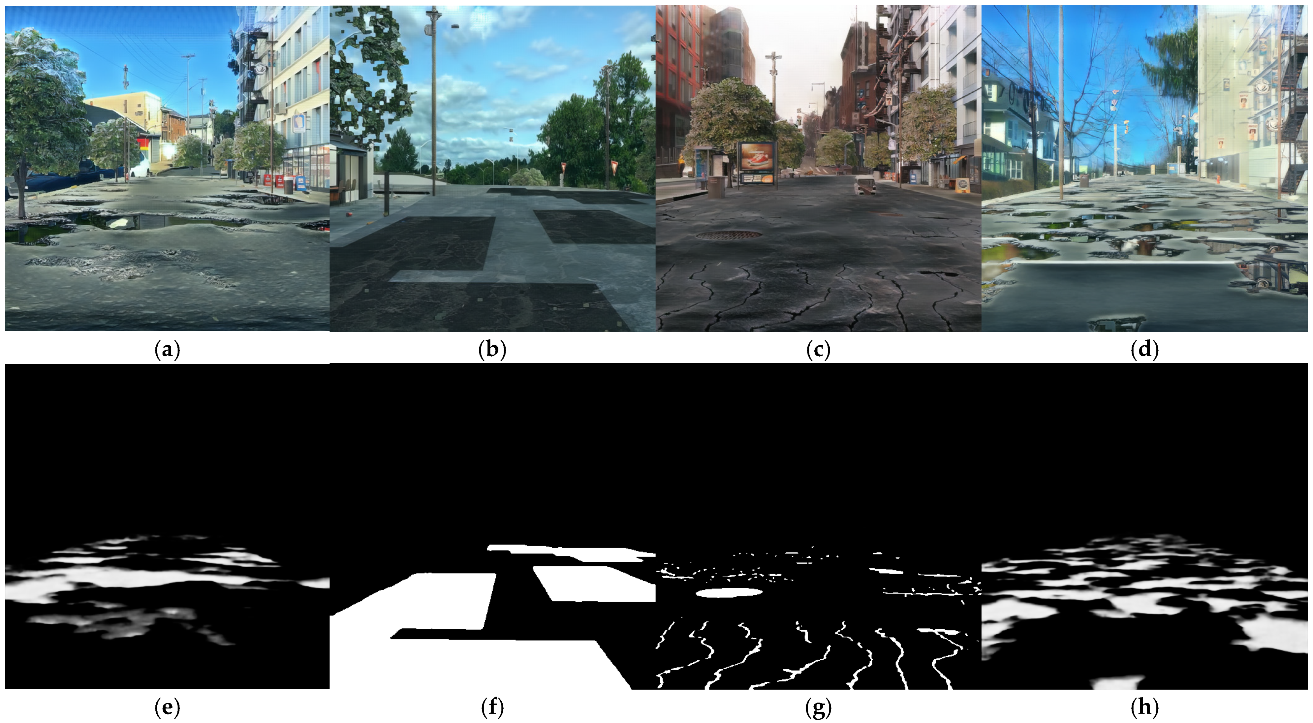
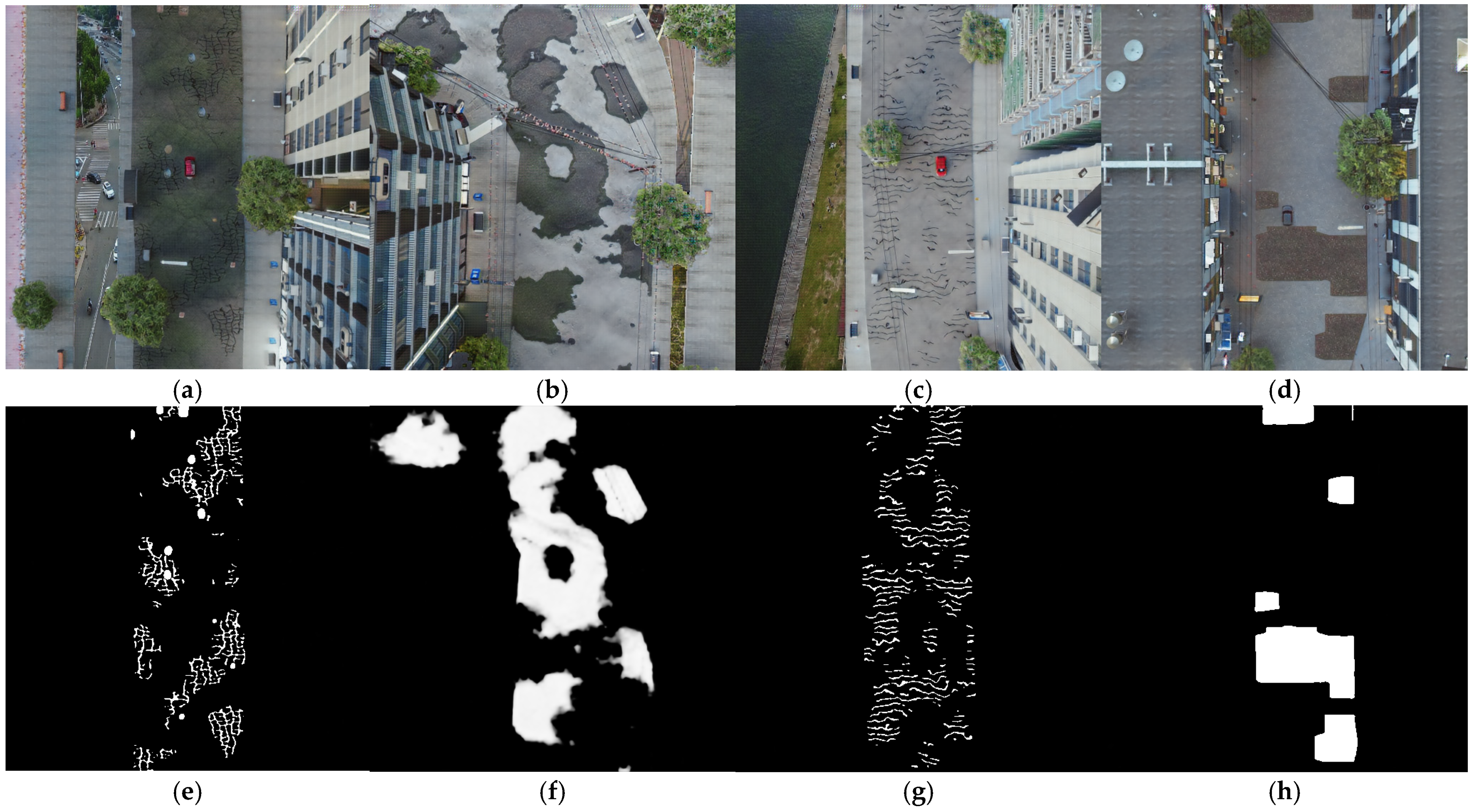
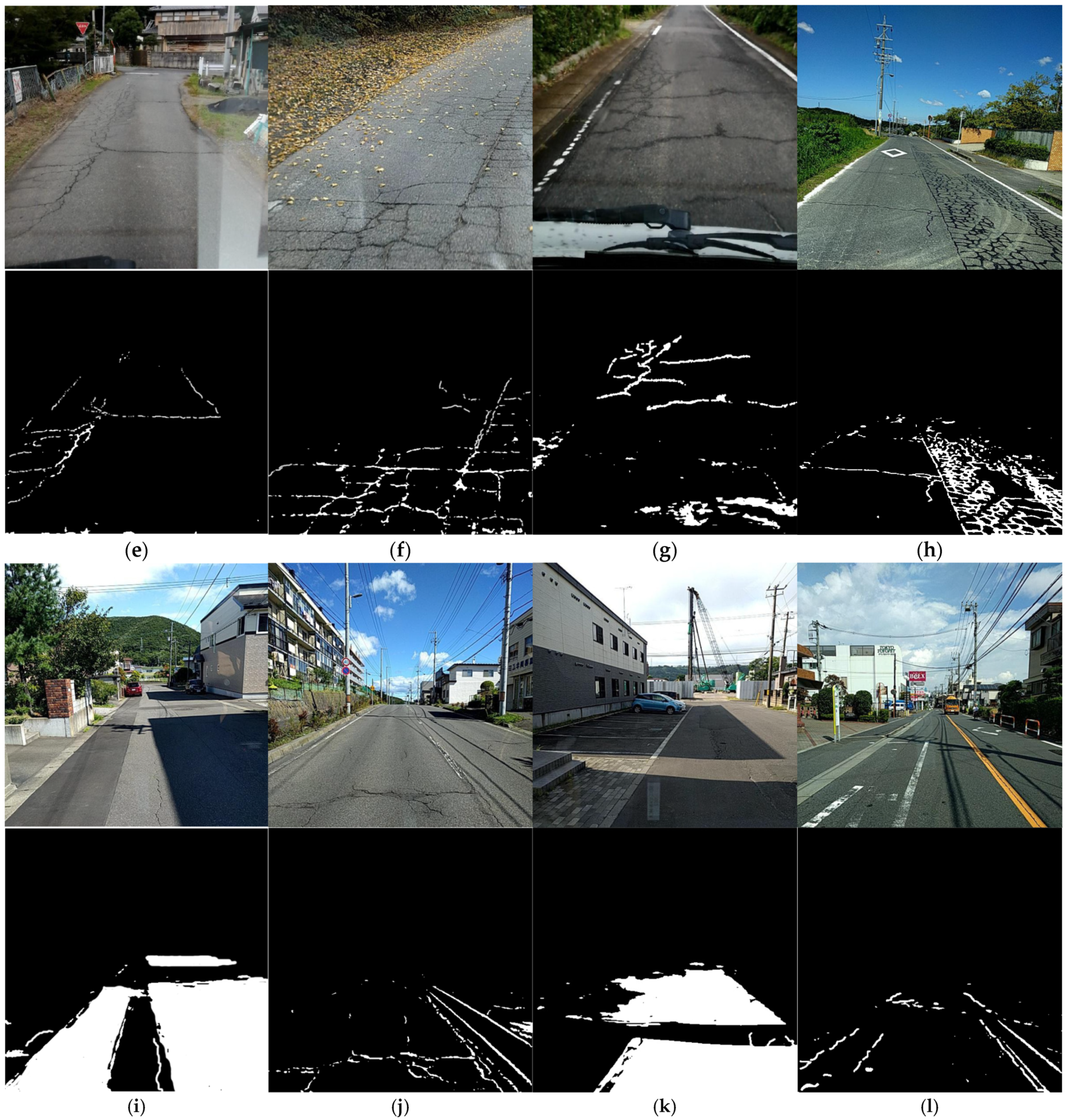
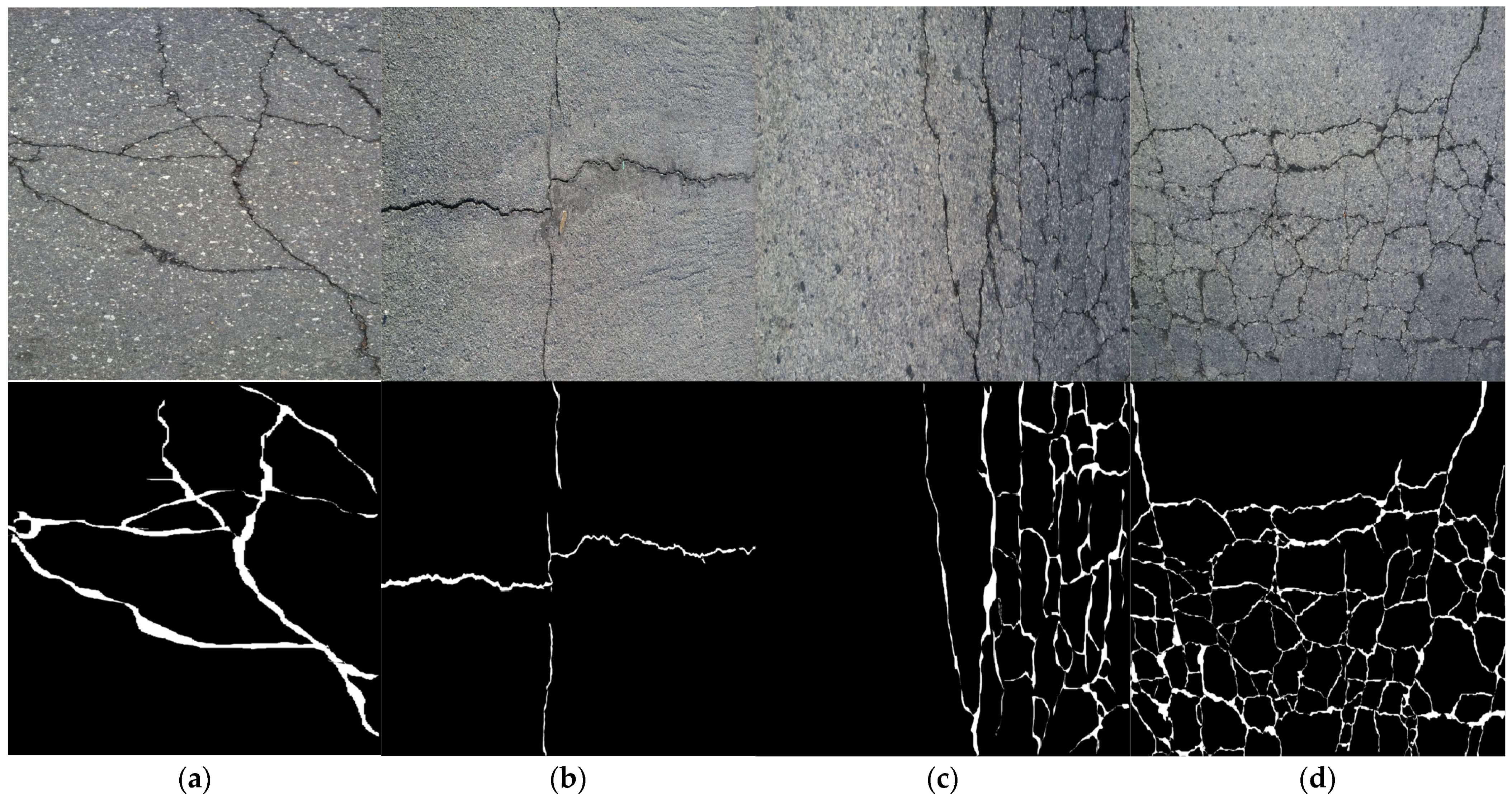
This study presented a novel two-stage deep learning framework for comprehensive road surface perception. The first stage, a segmentation-aware CycleGAN, effectively mitigated the synthetic-to-real domain gap by successfully translating synthetic images to a realistic domain while preserving defect fidelity (Figure 1). This crucial step enables the utilization of richly annotated synthetic data, addressing the inherent data acquisition bottleneck in real-world road defect analysis.

The second stage, our Modified DeepLabv3+ model, demonstrated robust multi-task performance in Table 1. It achieved strong segmentation accuracy for discrete defects, notably outperforming baseline DeepLabv3+ and other state-of-the-art models like PSPNet and SegFormer. Concurrently, it provided precise continuous defect severity and depth estimations. Although a marginal trade-off in the raw accuracy of continuous and depth predictions was observed compared to the DeepLabv3+ baseline, our model’s integrated multi-task capabilities offer a superior holistic understanding of road conditions, representing a favorable balance for comprehensive perception. Camera parameter estimation, while computationally challenging due to inherent ground-truth noise, consistently learned and provided reasonable estimations, as shown in Table 3, unlocking opportunities for calibration-free 3D reconstruction. The 3D reconstruction can be perfected using two consecutive frames which are much closer to each other rather than using monocular camera parameters from a single image. The model’s computational efficiency in Table 1 further supports its practical real-time deployment. Overall, this framework provides a scalable and accurate solution for road monitoring.

While our framework demonstrates significant promise, several avenues for future work are identified:

• Robustness to Environmental Challenges: A current limitation is the model’s susceptibility to environmental artifacts like shadows and reflections. Also, we assume the road monitoring is usually best performed at daytime. Future work will focus on integrating shadow detection or illumination-invariant features. Furthermore, the synthetic dataset could be expanded to include more challenging real-world variations such as adverse weather effects (e.g., rain, snow) and low-light or night-time conditions to further improve robustness.
• Refinement of Geometric Prediction: While the model learns camera parameters from a single image, the extrinsic accuracy can be improved. Future investigation could incorporate geometric constraints or leverage temporal consistency from video sequences to reduce pose estimation errors and enhance 3D reconstruction fidelity.
• Lightweight Variants for Edge Deployment: Our current model achieves real-time performance on a high-end GPU. A crucial next step for practical ADAS integration is to explore lightweight model variants suitable for deployment on edge devices. This could involve techniques such as quantization, knowledge distillation, or designing a more compact architecture from the ground up.
• Expanded Domain Adaptation: Exploring advanced domain adaptation strategies could further mitigate residual synthetic-to-real discrepancies and improve generalization across a wider range of real-world datasets with more diverse environmental and lighting conditions.
• Ethical Considerations and Bias: To ensure fair and equitable societal impact, future work should address potential biases in the dataset and model. This includes ensuring the synthetic data represents a wide variety of global road types and conditions to prevent the model from performing better in certain geographic or socioeconomic areas than others.
• Adversarial Robustness: A broader consideration for deployment in safety-critical applications is the model’s resilience to adversarial attacks. Research has shown that deep learning models can be vulnerable to carefully crafted perturbations designed to cause misclassification [31]. This represents an important direction for future investigation to ensure system reliability.

7. Conclusions

This paper introduced a novel two-stage deep learning framework for advanced road surface perception, addressing critical challenges in autonomous driving and infrastructure management through the strategic utilization of synthetic data. Our core contributions include a large-scale, procedurally generated 3D synthetic dataset with pixel-perfect multi-task annotations, a multi-task DeepLabv3+-based framework for joint defect segmentation, continuous severity estimation, depth prediction, and camera parameter estimation, and a novel two-stage domain adaptation pipeline. The proposed system demonstrated high accuracy and computational efficiency in benchmarking experiments. The segmentation aware CycleGAN effectively translated synthetic images to a realistic domain while preserving defect fidelity, showcasing a robust solution for the sim-to-real gap. The Modified DeepLabv3+ achieved competitive segmentation accuracy (mIoU of 0.7852) and precise continuous/depth predictions, outperforming several SOTA models in our multi-task setup. The capability to estimate camera parameters simultaneously enables unique opportunities for calibration-free 3D reconstruction of the road environment. While camera parameter estimation presented unique optimization challenges, its integration provides a path towards comprehensive geometric understanding.