
Enhanced Cuckoo Search Optimization with Opposition-Based Learning for the Optimal Placement of Sensor Nodes and Enhanced Network Coverage in Wireless Sensor Networks


Abstract
Featured Application
Abstract
1. Introduction
2. Contributions
2.1. Motivation
2.2. Main Contributions
- (a)
- The coverage model in the WSN is defined, and an objective function for the optimal coverage is established.
- (b)
- A “sequential update evaluation mechanism” is used, whereby each dimension is evaluated one by one, and this process mitigates the effect of dependency among dimensions and provides highly accurate solutions, particularly during the local search phase.
- (c)
- During the preference random walk phase of conventional CSO, PSO with adaptive inertia weights is integrated with the ECSO-OBL algorithm. This improves the local search capabilities.
- (d)
- The OBL strategy is applied to have high-quality initial solutions that help to balance the exploration and exploitation strategies. By considering the opposite of current solutions to expand the search space, we achieve higher convergence speed and population diversity.
3. Existing Works
4. The Proposed ECSO-OBL Algorithm
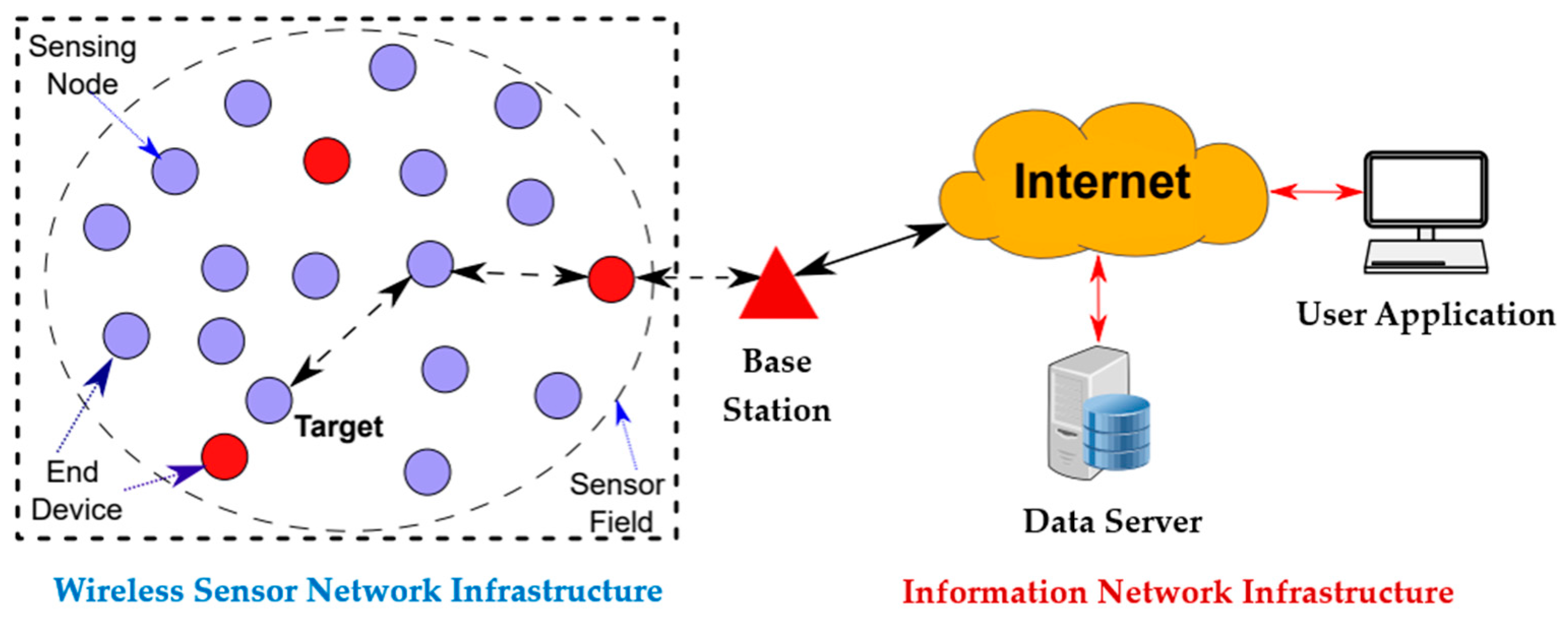
4.1. WSN Node Coverage Model
- (a)
- The sensing area of a sensor node is a circle with radius , and the node is located at the center.
- (b)
- All sensor nodes have the same processing and communication features.
- (c)
- The communication radius of each senor node is at least twice the sensing radius, i.e., .
- (d)
- When the sensor nodes are in motion, they update their location coordinates on a real-time basis.
4.2. Uni-Dimensional Update Mechanism
- Step 1: Define and configure the initial parameters, such as search space dimensions, number of nests, maximum number of iterations, and optimization problem dimensions.
- Step 2: In the given N-dimensional search space, generate the initial population (“S” number of nests) using Equation (4), and evaluate their individual fitness values.
- Step 3: Update the nest positions using Lévy flight, and retain the nests with higher fitness values as per Equation (5).where is the position of the nest for the generation and is the position of the nest for the generation. is the step control volume; , where lies between 1 and 3, represents the random search; is the random step size following a normal distribution; and is the pointwise multiplication operator.
- Step 4: Integrate the CSO with adaptive PSO to update the nest positions using the sequential update mechanism, as shown in Equations (6) and (7), and retain the nests with higher fitness values.where and → learning factors (they represent the social awareness and self-awareness of an individual nest); → inertia weight; and → optimal value of the nest from the to the generations. → optimal value among all nests in the generation; and → velocities of the nest in the and generations. and → positions of the nest in the and generations. and → random numbers [0, 1].
- Step 5: Apply “opposition-based learning” for the best 10% possible current solutions (whose fitness values are the highest), and generate their corresponding opposite solutions by using Equation (11). Accordingly, update the current nest positions, and retain the nests with the highest fitness values.where → search space boundary in the dimension; → multiplication factor in the range [0, 1]; → set of the best current solutions; and → set of the inverse solutions.
- Step 6: The algorithm stops executing once it meets the termination condition, and it gives best possible solution as output; otherwise, it moves to step 3.
4.3. Cluster Head Selection Using ECSO-OBL Algorithm
- Initial cluster vertices are produced randomly using Levi’s flight path.
- Initially, 10% of the total sensor nodes are selected as the best CHs, and the fitness function is used to assess their quality.
- Based on the fitness function, the solutions are revised if their quality is higher than the current solution.
- With the support of Levi’s flight, the worst nests are discarded and rebuilt in a new location.
- This procedure is continued until the termination condition is satisfied, and the algorithm execution is concluded.
| Algorithm 1. The proposed ECSO-OBL algorithm |
| Start |
| For i = 1 to N /* N → Total number of target nodes (TN) |
| Select each TN; |
| Perform AN selection; /* AN → anchor node |
| Compute distance between TN and each selected AN; |
| Assign weights to ANs; |
| Define the fitness function; |
| Define the range of : set ; |
| Generate initial set of solutions, , k = 1, 2, 3, ……R; |
| Define the range of solutions: ; |
| While do /* → Maximum number of iterations |
| For each do |
| If then |
| ; Else if then |
| ; |
| End if; |
| Set as current global optimal fitness value; |
| Calculate according to Equation (13); |
| Generate a fraction of as new solutions; |
| Compute the objective function; |
| Evaluate the fitness of the objective function; |
| End for; |
| End While; |
| End for; |
| Derive the new set of best or optimal solutions; |
| Arrange the solutions to find the best of them; |
| End |
5. Results and Discussions
6. Conclusions and Future Work
Author Contributions
Funding
Institutional Review Board Statement
Informed Consent Statement
Data Availability Statement
Acknowledgments
Conflicts of Interest
Abbreviations
| ACSO | Adaptive CSO |
| AN | Anchor node |
| CD | Cauchy distribution |
| CSO | Cuckoo search optimization |
| ICS | Improved cuckoo search |
| IoT | Internet of Things |
| LEACH | Low-energy adaptive clustering hierarchy |
| OBL | Opposition-based learning |
| PSO | Particle swarm optimization |
| ROI | Region of interest |
| TN | Target node |
| WSN | Wireless sensor networks |
References
- Ojeda, F.; Mendez, D.; Fajardo, A.; Ellinger, F. On Wireless Sensor Network Models: A Cross-Layer Systematic Review. J. Sens. Actuator Netw. 2023, 12, 50. [Google Scholar] [CrossRef]
- Shaikh, M.S.; Wang, C.; Xie, S.; Zheng, G.; Dong, X.; Qiu, S.; Ahmad, M.A.; Raj, S. Coverage and connectivity maximization for wireless sensor networks using improved chaotic grey wolf optimization. Sci. Rep. 2025, 15, 15706. [Google Scholar] [CrossRef] [PubMed]
- Tran, S.; Phan, D.M.; Vu, H.N.M.; Hoang, A.; Hoang, D.C. Alternative Nature-Inspired Optimizers: An Attempt to Solve the Coverage and Connectivity Problem in Wireless Sensor Network Deployment. In Proceedings of the International Conference on Intelligent Systems and Networks, Hanoi, Vietnam, 22–23 March 2024; ICISN 2024. Lecture Notes in Networks and Systems. Volume 1077, pp. 318–326. [Google Scholar] [CrossRef]
- Shalu, S.; Manjeet, S. Coverage and Connectivity in WSN: A Review. In Artificial Intelligence and Communication Technologies; Hiranwal, S., Mathur, G., Eds.; SCRS: Delhi, India, 2023; pp. 697–704. [Google Scholar] [CrossRef]
- Mohsen, S.H.; Seyed, R.S.H. Connectivity and coverage constrained wireless sensor nodes deployment using steepest descent and genetic algorithms. Expert Syst. Appl. 2022, 190, 116164. [Google Scholar] [CrossRef]
- Amer, D.A.; Soliman, S.A.; Hassan, A.F.; Zamel, A.A. Enhancing connectivity and coverage in wireless sensor networks: A hybrid comprehensive learning-Fick’s algorithm with particle swarm optimization for router node placement. Neural Comput. Applic 2024, 36, 21671–21702. [Google Scholar] [CrossRef]
- Hadir, A.; Kaabouch, N. Accurate Range-Free Localization Using Cuckoo Search Optimization in IoT and Wireless Sensor Networks. Computers 2024, 13, 319. [Google Scholar] [CrossRef]
- Ameed, M.K.; Idrees, A.K. Cuckoo Scheduling Algorithm for Lifetime Optimization in Sensor Networks of IoT. In Inventive Systems and Control: Proceedings of ICISC 2021, Coimbatore, India, 7–8 January 2021; Suma, V., Chen, J.I.Z., Baig, Z., Wang, H., Eds.; Lecture Notes in Networks and Systems; Springer: Singapore, 2021; Volume 204, pp. 171–187. [Google Scholar] [CrossRef]
- Yang, J.; Xia, Y. Coverage and Routing Optimization of Wireless Sensor Networks Using Improved Cuckoo Algorithm. IEEE Access 2024, 12, 39564–39577. [Google Scholar] [CrossRef]
- Yang, S.; Xiang, Y.; Ahmad, S.Z.R.; Kang, D.; Zhou, K. An improved cuckoo search algorithm optimizes coverage in wireless sensor networks. Proc. Comput. Sci. 2023, 1, 0039. [Google Scholar] [CrossRef]
- Yang, S.-Y.; Xiang, Y.-H.; Kang, D.-W.; Zhou, K.-Q. An Improved Cuckoo Search Algorithm for Maximizing the Coverage Range of Wireless Sensor Networks. Baghdad Sci. J. 2024, 21, 568–583. [Google Scholar] [CrossRef]
- Bing, Z.; Youyou, L. Presenting a New Approach for Clustering Optimization in Wireless Sensor Networks using Fuzzy Cuckoo Search Algorithm. Int. J. Adv. Comput. Sci. Appl. 2024, 15, 245–257. [Google Scholar] [CrossRef]
- Li, Y.; Cao, J. WSN node optimal deployment algorithm based on adaptive binary particle swarm optimization. ASP Trans. Internet Things 2021, 1, 1–8. [Google Scholar] [CrossRef]
- Dao, T.-K.; Chu, S.-C.; Nguyen, T.-T.; Nguyen, T.-D.; Nguyen, V.-T. An Optimal WSN Node Coverage Based on Enhanced Archimedes Optimization Algorithm. Entropy 2022, 24, 1018. [Google Scholar] [CrossRef]
- Tushar, K.S.; Sushree, C.P.; Manas, R.K. An adaptive cuckoo search based algorithm for placement of relay nodes in wireless body area networks. J. King Saud. Univ.—Comput. Inf. Sci. 2022, 34, 1845–1856. [Google Scholar] [CrossRef]
- Yarinezhad, R.; Hashemi, S.N. A sensor deployment approach for target coverage problem in wireless sensor networks. J. Ambient. Intell. Hum. Comput. 2023, 14, 5941–5956. [Google Scholar] [CrossRef]
- Nematzadeh, S.; Mahsa, T.-A.; Amir, S.; Farzad, K. Maximizing Coverage and Maintaining Connectivity in WSN and Decentralized IoT: An Efficient Metaheuristic-Based Method for Environment-Aware Node Deployment. Neural Comput. Appl. 2022, 35, 611–641. [Google Scholar] [CrossRef]
- Xu, Y.; Zhang, B.; Zhang, Y. Application of an Enhanced Whale Optimization Algorithm on Coverage Optimization of Sensor. Biomimetics 2023, 8, 354. [Google Scholar] [CrossRef]
- Tian, M.; Bai, J.; Li, J.; Huang, M.; Zhan, C.; Ren, L. Elite Parallel Cuckoo Search Algorithm for Regional Coverage Control Problem in High-Density Wireless Sensor Networks. In Proceedings of the 2021 3rd International Conference on Artificial Intelligence and Advanced Manufacture (AIAM), Manchester, UK, 23–25 October 2021; pp. 285–289. [Google Scholar] [CrossRef]
- Ajam, L.; Nodehi, A.; Mohamadi, H. A new approach to solving target coverage problem in wireless sensor networks using an effective hybrid genetic algorithm and tabu search. J. Intell. Fuzzy Syst. 2021, 42, 6245–6255. [Google Scholar] [CrossRef]
- Arivudainambi, D.; Pavithra, R.; Kalyani, P. Cuckoo search algorithm for target coverage and sensor scheduling with adjustable sensing range in wireless sensor network. J. Discret. Math. Sci. Cryptogr. 2020, 24, 975–996. [Google Scholar] [CrossRef]
- Chen, Z.; Cheng, J.; He, M. Coverage optimization in wireless sensor network based on multi-strategy dung beetle optimization algorithm. Evol. Intell. 2025, 18, 56. [Google Scholar] [CrossRef]
- Pavithra, R.; Arivudainambi, D. Coverage-Aware Sensor Deployment and Scheduling in Target-Based Wireless Sensor Network. Wirel. Pers. Commun. 2023, 130, 421–448. [Google Scholar] [CrossRef]
- Di Puglia Pugliese, L.; Guerriero, F.; Mitton, N. Optimizing wireless sensor networks deployment with coverage and connectivity requirements. Ann. Oper. Res. 2025, 346, 1997–2008. [Google Scholar] [CrossRef]
- Gandomi, A.H.; Yang, X.S.; Alavi, A.H. Cuckoo search algorithm: A metaheuristic approach to solve structural optimization problems. Eng. Comput. 2013, 29, 17–35. [Google Scholar] [CrossRef]
- Ding, J.; Wang, Q.; Zhang, Q.; Ye, Q.; Ma, Y. A Hybrid Particle Swarm Optimization-Cuckoo Search Algorithm and Its Engineering Applications. Math. Probl. Eng. 2019, 2019, 5213759. [Google Scholar] [CrossRef]
- Zheng, H.Q.; Feng, W.J. An improved Cuckoo Search algorithm for Constrained Optimization Problems. Chin. J. Eng. Math. 2023, 40, 135–146. [Google Scholar] [CrossRef]
- Houssein, E.H.; Saad, M.R.; Djenouri, Y.; Hu, G.; Ali, A.A.; Shaban, H. Metaheuristic algorithms and their applications in wireless sensor networks: Review, open issues, and challenges. Cluster Comput. 2024, 27, 13643–13673. [Google Scholar] [CrossRef]
- Pushpa, G.; Babu, R.A.; Subashree, S.; Senthilkumar, S. Optimizing coverage in wireless sensor networks using deep reinforcement learning with graph neural networks. Sci. Rep. 2025, 15, 16681. [Google Scholar] [CrossRef] [PubMed]


| Ref. | Authors | Objective | Methodology | Limitations |
|---|---|---|---|---|
| [9] | Yang and Xia (2024) | Design routing and coverage optimization in WSNs using improved CSO and non-uniform clustering. | Coverage optimization is addressed through Cauchy distribution. The average coverage is 96%. | The algorithm’s minimum run time is 1.47 min, with an energy loss rate of 0.84%. |
| [10] | Yang et al. (2023) | Maximize network coverage using a hybrid algorithm that combines CSO and PSO. | Convert the regional monitoring space into point monitoring space by using discretization methods. | Though the coverage rate of the proposed algorithm is enhanced by 18.36% compared with CSO, it enters an early stagnation state and is trapped in a local optimal solution. For all the network sizes, the accuracy and convergence speed are inferior. |
| [11] | Yang et al. (2024) | Increase network coverage by using a hybrid CSO-PSO algorithm and “opposition-based learning (OBL)”. | The OBL strategy broadens search space exploration to improve the diversity of the population. | The convergence time of the hybrid CSO-PSO algorithm is too high. |
| [12] | Bing and Youyou (2024) | Hybrid combination of LEACH and CSO to improve network lifetime and packet delivery ratios. | During clustering and cluster head selection, the LEACH protocol uses CSO. During the routing phase, fuzzy logic is used. | Performance is dependent on the distance between mobile and stationary sensors nodes. |
| [13] | Li and Cao (2021) | Improve the coverage rate in WSNs using discrete binary PSO. | For optimal deployment, an adaptive learning factor and inertia weights are introduced. | The coverage ratio decreases as the dimensions of the network increase. |
| [14] | Dao et al. (2022) | Use “Archimedes optimization” for optimal coverage in an unbalanced WSN distribution. | “Reverse learning” and “multidirectional” techniques are introduced. Coverage optimization is implemented through the evaluation of fitness per sub-area. | It falls into local minima and has a slow convergence rate. |
| [15] | Tushar et al. (2022) | Minimize the cost and energy consumption of relay nodes with uniform load distribution. Used for optimal placement and selection of relay nodes when using adaptive CSO in body area networks. | Optimal placement of relay nodes and routing are formulated as “a linear integer programming” model. CSO with an adaptive step size is defined. The fitness function is defined based on coverage, load, and energy consumption of the sensors nodes. | It is time-consuming due to the fixed relay nodes while starting and then increases to identify the optimal number. The search space is increased exponentially and causes higher execution time, and it further increases with network size. |
| [16] | Ramin and Seyed (2020) | The coverage problem is modeled to enhance the network lifetime. | Cooperative PSO and fuzzy logic are used to solve the node deployment problem. Fuzzy logic computes acceleration coefficients on a dynamic basis and enhances network lifetime. | The solution is limited to cover fixed target nodes, and the resolution of the coverage is poor. |
| [17] | Sajjad et al. (2022) | Node deployment problem is addressed using metaheuristic approach. | Mutant-GWO model ensures connectivity by generating topology graphs. | Power consumption is too high due to collisions. |
| [18] | Xu et al. (2023) | Coverage optimization problem in WSNs. | Whale optimization with Lévy flight and genetic algorithm is used. | Though the coverage rate is 90.33%, the complexity of this algorithm is too high. |
| [19] | Tian et al. (2021) | Regional coverage control in high-density WSNs is addressed. | Elite parallel CSO, which is randomized swarm optimization, is introduced. | It has a slow convergence rate and is not suitable for combinatorial optimization and discrete optimization problems. |
| [20] | Ajam et al. (2021) | Proposed to maximize network lifetime with variable ranges. | Hybrid combination of “Genetic Algorithm” and “Tabu Search” used to define cover sets with suitable sensing ranges. | This algorithm is not suitable for uniform WSNs. |
| [21] | Arivudainambi et al. (2020) | Optimize the sensing range by minimizing redundancy in WSNs. | Based on the sensing range, the CSO algorithm classifies the sensor nodes into non-disjoint subsets. At a given time, only one subset is activated to cover the network area. The activation of each subset is in cycles to enhance the network lifetime. | Convergence time is too high. |
| [22] | Chen et al. (2025) | Enhance and optimize coverage in 2D and 3D WSNs. | Multi-strategy dung beetle optimization algorithm that uses a random number to change the inertia factor. | The maximum coverage is limited to 77.7%. |
| [23] | Pavithra and Arivudainambi (2023) | Energy-efficient target coverage in WSNs. | Energy-efficient coverage is described as a set k-cover problem with independent sensor sets, and it is solved using graph theory. | The range of sensing is fixed, and it leads to lower energy efficiency. |
| [24] | Di Puglia et al. (2025) | Deploy minimum count of sensor nodes to fully cover the ROI and enhance connectivity. | The proposed method is described as a “connectivity problem” and a “covering problem”. It is solved using decomposition techniques based on the “Miller-Tucker-Zemlin” model. | It takes a greater number of iterations and execution time to achieve optimal results. |
| Processor configuration | 12th Gen Intel Core i7-12700, 2.1 GHz |
| Operating system | Windows 11 (Microsoft) Enterprise |
| System model | HP Pro Tower 400 G9 PCI |
| System type | x64-based PC |
| Physical RAM | 16 GB |
| Network Parameter | Values | ||
|---|---|---|---|
| Case 1 | Case 2 | Case 3 | |
| Network terrain dimensions | 50 m2 | 100 m2 | 200 m2 |
| Network size (in terms of number of sensor nodes, N) | 20 | 40 | 80 |
| Sensing radius | 6 m | 8 m | 10 m |
| Communication radius | 12 m | 16 m | 20 m |
| Carrier frequency | 39 GHz | 39 GHz | 39 GHz |
| Number of iterations | 100 | 200 | 300 |
| Parameters of the various algorithms and their initialization | |||
| CSO [23] | |||
| CD-CSO [9] | |||
| ACSO [15] | |||
| PSO-CSO [10] | |||
| ICS-PSO-OBL [11] | |||
| ECSO-OBL [proposed] | |||
| Function | Definition | Interval |
|---|---|---|
| Beale | [−4.5 4.5] | |
| Rosenbrock | [−30 30] | |
| Step | [−100 100] | |
| Sphere | [−5.12 5.12] | |
| Rastrigin | [−5.12 5.12] | |
| Schwefel | [−100 100] | |
| Griewank | [−600 600] | |
| Schaffer | [−100 100] |
| Metric | Algorithm | Network Dimensions | ||
|---|---|---|---|---|
| 50 m2 | 100 m2 | 200 m2 | ||
| N | 20 | 40 | 80 | |
| Iterations for convergence | ICS-PSO-OBL [11] | 158 | 194 | 417 |
| CD-CSO [9] | 147 | 181 | 436 | |
| ACSO [15] | 182 | 214 | 524 | |
| PSO-CSO [10] | 226 | 289 | 559 | |
| ECSO-OBL [proposed] | 112 | 143 | 314 | |
| Execution time (sec) | ICS-PSO-OBL [11] | 4.14 | 8.25 | 11.3 |
| CD-CSO [9] | 3.95 | 7.19 | 10.4 | |
| ACSO [15] | 4.15 | 8.49 | 9.48 | |
| PSO-CSO [10] | 3.83 | 6.41 | 9.16 | |
| ECSO-OBL [proposed] | 2.26 | 2.85 | 6.02 | |
| Maximum coverage rate (%) | ICS-PSO-OBL [11] | 83.42 | 84.39 | 86.31 |
| CD-CSO [9] | 84.46 | 91.34 | 92.38 | |
| ACSO [15] | 78.13 | 80.38 | 85.13 | |
| PSO-CSO [10] | 82.75 | 88.42 | 89.35 | |
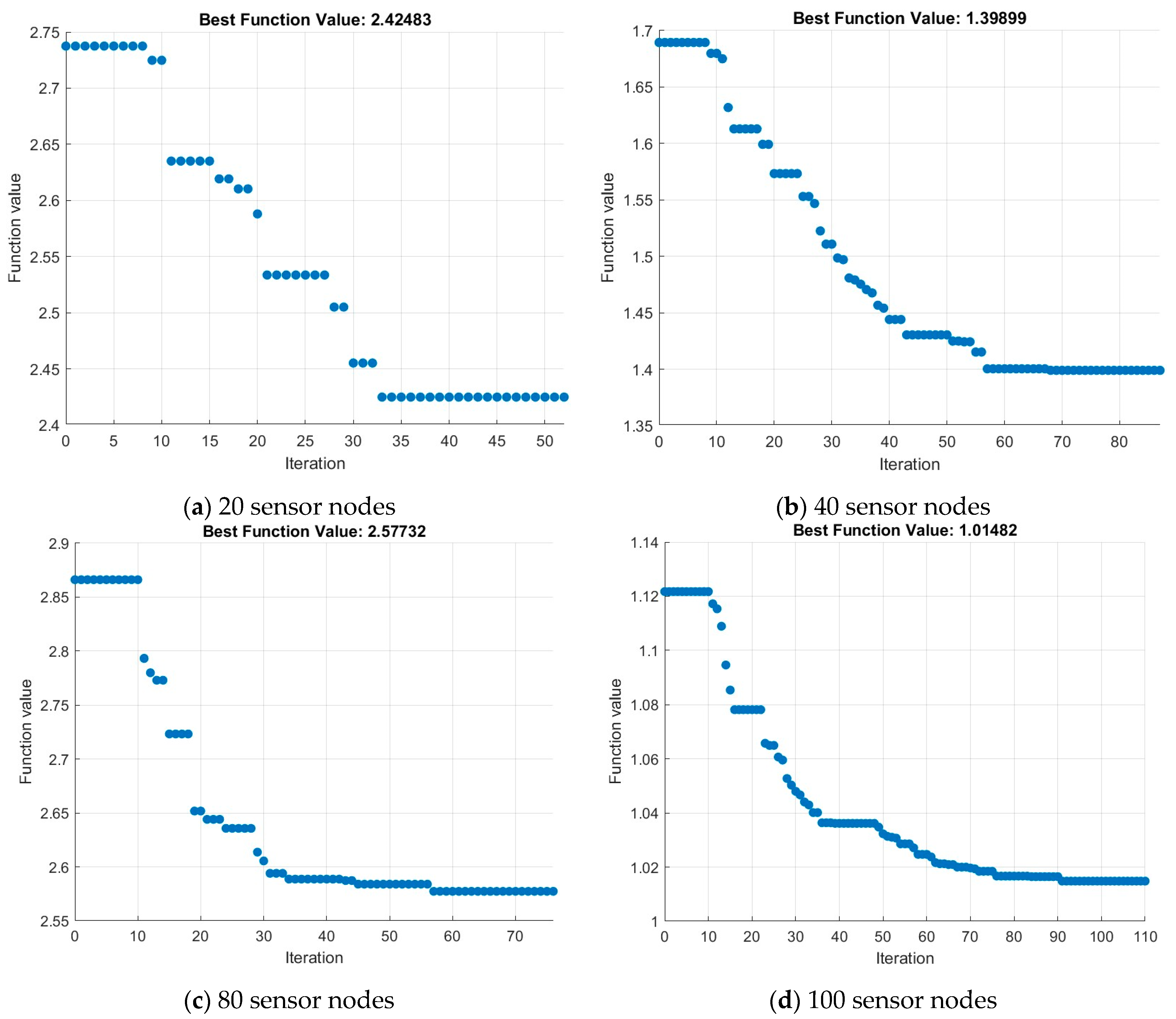
| ECSO-OBL [proposed] | 96.42 | 98.45 | 96.21 | |
| Fitness values | ICS-PSO-OBL [11] | 1.0109 | 1.0005 | 1.0318 |
| CD-CSO [9] | 1.0125 | 1.0813 | 1.0159 | |
| ACSO [15] | 1.0064 | 1.0071 | 1.0048 | |
| PSO-CSO [10] | 1.0137 | 1.0022 | 1.0039 | |
| ECSO-OBL [proposed] | 2.42483 | 1.3989 | 2.57732 | |
Disclaimer/Publisher’s Note: The statements, opinions and data contained in all publications are solely those of the individual author(s) and contributor(s) and not of MDPI and/or the editor(s). MDPI and/or the editor(s) disclaim responsibility for any injury to people or property resulting from any ideas, methods, instructions or products referred to in the content. |
© 2025 by the authors. Licensee MDPI, Basel, Switzerland. This article is an open access article distributed under the terms and conditions of the Creative Commons Attribution (CC BY) license (https://creativecommons.org/licenses/by/4.0/).
Share and Cite
Reddy, M.R.; Chandra, M.L.R.; Dilli, R. Enhanced Cuckoo Search Optimization with Opposition-Based Learning for the Optimal Placement of Sensor Nodes and Enhanced Network Coverage in Wireless Sensor Networks. Appl. Sci. 2025, 15, 8575. https://doi.org/10.3390/app15158575
Reddy MR, Chandra MLR, Dilli R. Enhanced Cuckoo Search Optimization with Opposition-Based Learning for the Optimal Placement of Sensor Nodes and Enhanced Network Coverage in Wireless Sensor Networks. Applied Sciences. 2025; 15(15):8575. https://doi.org/10.3390/app15158575
Chicago/Turabian StyleReddy, Mandli Rami, M. L. Ravi Chandra, and Ravilla Dilli. 2025. "Enhanced Cuckoo Search Optimization with Opposition-Based Learning for the Optimal Placement of Sensor Nodes and Enhanced Network Coverage in Wireless Sensor Networks" Applied Sciences 15, no. 15: 8575. https://doi.org/10.3390/app15158575
APA StyleReddy, M. R., Chandra, M. L. R., & Dilli, R. (2025). Enhanced Cuckoo Search Optimization with Opposition-Based Learning for the Optimal Placement of Sensor Nodes and Enhanced Network Coverage in Wireless Sensor Networks. Applied Sciences, 15(15), 8575. https://doi.org/10.3390/app15158575