Leveraging Feature Extraction to Perform Time-Efficient Selection for Machine Learning Applications

Abstract

In the age of rapidly advancing machine learning capabilities, the pursuit of maximum performance encounters the practical limitations imposed by limited resources in several fields. This work presents a cost-effective proposal for feature selection, which is a crucial part of machine learning processes, and intends to partly solve this problem through computational time reduction. The proposed methodology aims to strike a careful balance between feature exploration and strict computational time concerns, by enhancing the quality and relevance of data. This approach focuses on the use of interim representations of feature combinations to significantly speed up a potentially slow and computationally expensive process. This strategy is evaluated in several datasets against other feature selection methods, and the results indicate a significant reduction in the temporal costs associated with this process, achieving a mean percentage decrease of 85%. Furthermore, this reduction is achieved while maintaining competitive model performance, demonstrating that the selected features remain effective for the learning task. These results emphasize the method’s feasibility, confirming its ability to transform machine learning applications in environments with limited resources.

1. Introduction

Machine learning (ML) has achieved a prominent position in recent years. Much of its recent visibility may be attributed to large volumes of data (used for training purposes) as well as improved computing infrastructure [1], giving rise to compelling applications like DALL-E https://openai.com/index/dall-e/ (accessed on 13 January 2025) [2] and ChatGPT https://openai.com/index/chatgpt/ (accessed on 13 January 2025) [3].

However, this also means greater importance is placed on this step of the ML pipeline than ever before. Data collecting is becoming one of the main bottlenecks in the field. The majority of the time for executing ML end-to-end is spent on preparing the data, which includes gathering, cleaning, analyzing, visualizing, and feature engineering [1].

This only exacerbates already existing related issues, such as the cold-start problem that is observable in certain fields, such as the medical field [4], e-commerce [5], and online education [6]. Manually labeling a dataset is very costly and complex. This is particularly true for research domains like healthcare that have limited access to labeled data [4]. To abstract underlying patterns and create a proper model, approaches often require massive amounts of supervised training data per inherent concept [7]. These learning processes can take days using specialized (and expensive) hardware [7].

One should recognize that there are applications for which data are inherently expensive to acquire, whether due to financial constraints or time limitations, making the development of suitable models for these fields a significant challenge [4].

These challenges mirror similar issues found in the field of digital marketing, where understanding human interaction across the physical and digital worlds requires selecting relevant tools and techniques that ensure flexibility and context-awareness [8,9]. Multi-modal artificial intelligence approaches have demonstrated the importance of integrating diverse data sources to analyze consumer sentiment and enhance engagement [10,11]. However, the complexity of integrating these modalities underscores the importance of efficient data pre-processing, including cost-effective feature selection, to reduce noise and improve the robustness of ML models [12].

Furthermore, these are not the only problems present in this context. Even if valuable data are sourced to be used for one of these aforementioned fields, current features may be redundant or even irrelevant to the problem at hand, which means that they only add noise to the dataset [12].

In order to deal with these problems, a data engineer may turn their attention to either the data or the algorithms that use them. That is, one may try to use approaches that require less data to obtain results, such as few or even zero-shot algorithms [7]. Or one may dedicate more attention to the data and try to improve them by iteratively cleaning and analyzing them.

This work addresses the challenge of balancing effective feature exploration with computational efficiency through a novel data-centric approach. We propose a feature selection method that accelerates the traditionally time-intensive wrapper-based feature selection process by leveraging interim representations of feature combinations. These composite representations enable the method to approximate inter-feature dependencies while relying on filter-based evaluation, resulting in a substantial reduction in computational time without maintaining competitive performance. The core novelty of our approach lies in its ability to deliver wrapper-like effectiveness with filter-level efficiency, making it particularly suitable for resource-constrained machine learning scenarios. To support and contextualize our contribution, we also present a brief review of dimensionality reduction and its two key branches: feature selection and feature extraction.

The paper follows the following structure. Initially, a concise overview of fundamental principles related to dimensionality reduction is presented, as well as a short description of relevant feature selection approaches used in testing (Section 2). Subsequently, the recommended solution is introduced and described (Section 3). After that, the results generated by this solution are compared to other presented approaches in terms of both temporal cost and performance (Section 4). Finally, conclusions are drawn, and future work is delineated (Section 5).

2. Dimensionality Reduction

Dimensionality reduction methods seek to improve data quality by lowering their complexity, therefore solving the phenomenon commonly referred to as the “curse of dimensionality”. (The term “curse of dimensionality” refers to the “blind spots” created by contiguous areas of feature space devoid of observations, which are found when working in datasets with high-dimensional data without expanding the sample size. This means the data to solve the topical problem become sparse, which makes extracting meaningful results difficult. This problem is commonly observed in real contexts [13]). They fall mostly into two categories: feature selection and feature extraction [14,15]. A diagram summarizing the core concept hierarchy for this knowledge field is presented in Figure 1. In this section, a short overview of the state of the art for both categories is provided and some of the included techniques are presented. Special attention is given to feature selection methods, as they are used for testing purposes later in this document.

2.1. Feature Selection

Feature selection is a critical step in both data engineering and machine learning workflows. This process is recognized as the selection of a subset from an initial feature set, guided by specified selection criteria [16,17].

By creating a smaller/more concise subset of relevant features using a suitable selection criterion, it is viable to reduce a problem’s scale (the quantity of data involved) while simplifying the process of analyzing it. This results in improving learning accuracy and potentially speeding up the learning process [16,18].

These outcomes are desirable since the volume of high-dimensional data has caused significant issues in the field. Due to the significant increases in sample size and dimensionality in the majority of ML use cases (e.g., the constant need to scale up large language models), this leads to the need for more computation time, more intricate models, and potentially more expensive hardware [16,18].

The main problems caused by this dimensional issue are related to the existence of noisy, redundant, or unnecessary dimensions. By creating representative subsets of the main datasets that eliminate the main sources of noise/redundancy, it is expected that the preceding issues would be solved [18]. Feature selection methods can be classified by taking into account different standards [15,16,18,19]:

• Label Information—This standard relates to the presence of label information in the data provided to the method. Supervised approaches use label information to select relevant features to adequately distinguish samples from different classes. Semi-supervised methods also attempt to find relevant features to differentiate between classes; however, due to the limited availability of labeled data, they exploit both labeled and unlabeled data. In general, it is considered that feature selection for unsupervised problems is a more challenging task than in the two previous cases [13,20,21]. The purpose of feature selection for unsupervised learning is to locate the feature subsets that reveal natural clusters in the processed data, according to the given selection criterion.
• Learning Method Relation—Feature selection techniques can be categorized as filter, wrapper, or embedded methods, based on their integration with the learning algorithm. Wrapper approaches assess the optimal feature subset using the underlying ML algorithm. The performance metric used to assess the final model may serve as the selection criterion, and multiple passes may be used to reach an optimal feature set. Filter methods select the relevant features through statistical characteristics intrinsically present in the data. They typically follow a two-step approach, with feature selection occurring before the machine learning algorithm (regardless of the objective being clustering or classification). In embedded methods, feature selection is inherent to the process of model construction. Various hybrid approaches fall under this classification.
• Evaluation Criterion—Feature subsets are selected based on various evaluation criteria. Commonly, the metrics used for evaluation are the Euclidean distance, consistency, dependence, and an information measure.
• Search Strategy—This standard is based on the general approach taken by the feature selection method. It divides techniques into forward selection, backward elimination, random, and hybrid models. Briefly, forward selection techniques build a subset by iteratively adding more relevant features to an initially empty one. Backward elimination, on the other hand, starts from the full feature set and iteratively eliminates features that are not considered relevant. Random approaches normally select a number of random feature subsets and then find the one with the best performance. Hybrid approaches combine any of the aforementioned approaches, or may even just take steps to improve them by including different techniques or algorithms in their process [22].
• Output Type—Feature selection methods may output either the feature subset that it considers best/most able to perform, or the feature ranking of the original data passed to it, meaning their relative importance according to the chosen approach.

The most commonly used differentiation standard for feature selection seems to be its relation with the learning method. Each group has their advantages and disadvantages.

Filter-based feature selection methods are computationally efficient and widely used across various domains. However, they typically assess each feature independently using statistical measures such as correlation with the target, chi-squared scores, or mutual information. This univariate approach overlooks interactions between features, meaning that features deemed irrelevant individually may be useful when combined [22].

Wrapper techniques address this limitation by searching much more thoroughly; however, this also means they are more computationally expensive [23,24]. Performance degradation is an entire research subject itself [22]. Embedded techniques integrate the process of selecting relevant features directly into the model training phase. This approach allows for simultaneous feature selection and model optimization, which can lead to improved model performance. However, since their performance is dependent on the learning algorithm, each has its own drawbacks [25,26].

2.2. Feature Extraction

Feature extraction is the process of converting high-dimensional data into a useful representation with reduced dimensionality. The dimensionality of the reduced representation should ideally match the intrinsic dimensionality of the data, which may be defined as the smallest number of factors required to explain its observable qualities [27,28]. This reduction is of benefit to the entire ML process. Feature extraction methods are commonly divided into linear and non-linear; however, more standards may be applied [14,27,29]:

• Label Information—Methods may be considered to be supervised or unsupervised. Supervised approaches take into consideration label information while processing data, while unsupervised ones infer solely from the data themselves. Most relevant feature extraction methods tend to be unsupervised.
• Data Linearity—According to this standard, methods are divided according to how data are combined on processing time. Linear techniques embed data into a lower-dimensional linear subspace for dimensionality reduction. Non-linear techniques transform a higher-dimensional space into a lower one non-linearly. The most common strategies to achieve this end are preserving global properties, preserving local properties, and performing global alignment of a mixture of linear models. Traditionally, linear techniques were used, but they struggle with complex non-linear data. Non-linear techniques offer a distinct advantage in modeling real-world data, which frequently involve complex, non-linear relationships.
• Data Topology—Certain techniques are designed to maintain the intrinsic relationships between data points during extraction. Random projection methods, for instance, use a randomly generated transformation matrix to project data into a lower-dimensional space while approximately preserving Euclidean distances. This is typically achieved by normalizing the matrix columns to unit length. In contrast, manifold learning approaches assume that high-dimensional data lie on a lower-dimensional, non-linear manifold. These methods, often unsupervised and graph-based, aim to uncover and embed this manifold in a way that preserves local neighbourhood relationships. Both types of techniques generate new data representations based on structural properties, complementing the traditional linear versus non-linear classification with a topology-aware view.
• Intrinsic Nature—Feature extraction techniques can also be characterized by the nature of the optimization problems they solve. In particular, convex approaches optimize objective functions that do not contain local optima, allowing these methods to reliably find a global solution. In contrast, non-convex methods may converge to one of multiple local optima, which can affect the stability and quality of the extracted features. While convexity pertains to the optimization process rather than the feature extraction technique itself, understanding this distinction provides insight into the computational complexity and solution reliability associated with different methods.

Regarding data linearity, in most cases, non-linear approaches appear to perform better than linear ones and manifold-based outperform random projection-based approaches, as seen in [14]. However, this is not always the case. In some cases, linear techniques (namely, principal component analysis) may outperform non-linear ones, as seen in [27].

Some relevant techniques in this area include the following [14,29,30]:

• Principal Component Analysis (PCA): PCA is a feature extraction technique used to reduce dimensionality by transforming features into a new set of uncorrelated variables, called principal components, which are ordered by the amount of variance they capture from the data. This technique identifies the directions in which the data varies the most and projects the data onto them. The key point of PCA is that it maximizes variance, capturing the most important aspects of the data structure.
• Linear Discriminant Analysis (LDA): LDA aims to preserve the class discriminatory information as much as possible. It finds the linear combinations of features that best separate two or more classes of objects or events. The key point of LDA is that it maximizes the ratio of the between-class variance to the within-class variance in the dataset, ensuring maximum class separability.
• Isometric mapping (ISOMAP): ISOMAP is a technique which aims to preserve the geodesic distances (shortest path distances on a manifold) between all points. It constructs a neighborhood graph and computes the shortest paths between all points, then applies Multidimensional Scaling (MDS) to these paths. The key point of Isomap is that it captures the underlying manifold structure of the data, making it useful for non-linear dimensionality reduction.

While these techniques are primarily used for feature extraction, some variants or applications may also utilize them to inform a feature selection process.

2.3. Feature Selection Algorithms

Before delving into the specifics of our approach, it is important to explore the metaheuristic and algorithmic strategies that are commonly employed in wrapper-based feature selection. These methods represent examples of the current state of the art and will later serve as reference points for assessing the performance of the proposed approach.

Metaheuristics were first proposed in order to define problems that can be applied to a large set of different problems (mainly optimization). What this means is that, generally speaking, a metaheuristic can be taken as a generic algorithm framework which may be applied to various optimization problems with a relative low amount of implementation effort. These are normally used to find good (but not necessarily optimal) solutions to complex optimization problems. Feature selection is often one of these application areas [31,32,33].

2.3.1. Binary Bat

The Binary Bat (BB) metaheuristic is based on the idea of simulating the echolocation behavior of bats. It was first presented in 2014 by Seyedali Mirjalili, Seyed Mohammad Mirjalili, and Xin-She Yang [34] as a binary version of the regular bat algorithm (BA). In BB, the bats are represented as agents that fly around a solution space, emitting sound waves and detecting the echoes to update their current positions [35,36].

The key steps involved in BB are the following [37]:

• Step 1: A population of bats with random positions and velocities is initialized.
• Step 2: Each bat emits a sound wave (a binary string) and detects the echo (the fitness value of the solution).
• Step 3: Each bat’s velocity is adjusted according to the echo and the loudness of the emitted wave.
• Step 4: Each bat’s position is updated based on its velocity.
• Step 5: Steps 2–4 are repeated until a stopping criterion is fulfilled, such as reaching a maximum number of iterations or achieving a satisfactory solution.

2.3.2. Cuckoo Search

The Cuckoo Search (CS) metaheuristic is inspired by the brood parasitism behavior of some cuckoo species [38]. It was first introduced by Xin-She Yangand Suash Deb in 2010 [39]. The algorithm is based on the cuckoo’s behavior of laying eggs in the nests of other birds, and the host birds’ behavior, which may discover these eggs and eject them or keep them [40]. It has been utilized for a variety of optimization problems, including feature selection [41,42].

CS follows three main rules/principles [38,40,41]:

1.

Each cuckoo randomly selects a nest to lay its eggs.

2.

The number of available host nests is constant, and nests with high-quality eggs are passed on to the next generation.

3.

If a host bird finds a cuckoo egg, it can either discard the egg or abandon the nest and construct a new one.

These principles are then translated to an algorithmic approximation so as to use them in real use cases. In such cases, the key steps involved in CS are the following [38,40,41]:

• Step 1: Various nests are initialized as a set of solutions. A set of eggs is initialized in each nest, each representing a solution.
• Step 2: A random nest is selected and a new egg (cuckoo’s egg) is generated by executing a “Levy Flight”, which involves random walks with step lengths derived from a heavy-tailed probability distribution, on its solution space. This new solution is then laid in this nest.
• Step 3: The fitness of this new egg is assessed using the fitness function in comparison to the existing eggs in the nest. If the new egg demonstrates better fitness than the least fit egg in the nest, it replaces that egg.
• Step 4: There exists a low chance of the host bird (function) detecting the cuckoo’s egg, in which case it may discard the egg or leave the nest, therefore avoiding local optimization.
• Step 5: Steps 2–4 are repeated until a stopping criterion is fulfilled, such as reaching a maximum number of iterations or attaining a satisfactory solution.

2.3.3. Equilibrium Optimizer

The Equilibrium Optimizer (EO) is an optimization algorithm, inspired by control volume mass balance models to estimate both dynamic and equilibrium states. It was first proposed by Afshin Faramarzi and Mohammad Heidarinejad in 2020 [43]. In EO, all particles (solutions) function as a search agent according to their concentration (position). These search agents adjust their concentration at random relative to the best-performing solutions (also known as equilibrium candidates) towards the equilibrium state (ideal outcome) [43,44]. EO has demonstrated the ability to randomly update the solution within a good balance between exploration and exploitation [45].

The key steps involved in EO are the following [43,44,45]:

• Step 1: An initial population of particles is randomly set up within the search space.
• Step 2: Each particle is evaluated using a fitness function, which assesses its performance and determines its suitability as an equilibrium candidate.
• Step 3: A selection of the top solutions from the current population is created based on their fitness values. These solutions are considered as equilibrium candidates and are expected to be nearer to the optimal solution.
• Step 4: For each candidate in the population (excluding the equilibrium candidates), their position is updated based on a randomly weighted influence of the equilibrium candidates from the equilibrium pool. This process helps to cover the entire search space and avoid local optima.
• Step 5: Whether any updated candidate solutions have gone out of the predefined bounds of the search space is checked. If so, boundary handling rules are applied to bring them back within valid limits.
• Step 6: Steps 2–5 are repeated until a stopping criterion is fulfilled, such as reaching a maximum number of iterations or attaining a satisfactory solution.

2.3.4. Genetic Algorithm

A Genetic Algorithm (GA) is a search-based optimization technique inspired by natural selection and genetics. This type of approach was popularized by John Henry Holland in the 1970s, especially through his book Adaptation in Natural and Artificial Systems [46]. These metaheuristics are part of the broader category of evolutionary algorithms (EA). GAs are commonly used to generate high-quality solutions to optimization and search problems by relying on biologically inspired operators. A GA repeatedly modifies a population of individual solutions, called individuals or phenotypes, to evolve toward better solutions. Each individual has a set of properties or chromosomes, that can be mutated and altered [47,48].

The key steps involved in GA are the following [47,48]:

• Step 1: An initial population of candidate solutions (chromosomes) is initialized in the search space.
• Step 2: These chromosomes are evaluated using a fitness function that measures the quality of the solution. After this, a subset of individuals from the population is selected based on their fitness values using a mechanism such as roulette wheel selection or tournament selection.
• Step 3: The selected chromosomes are combined to create a new solution by recombining their genetic information.
• Step 4: Random changes (mutations) are introduced to the offspring in order to increase their genetic diversity.
• Step 5: The least fit individuals in the population are replaced with the new offspring, creating a new generation.
• Step 6: Steps 2–5 are repeated until a stopping criterion is reached, such as a maximum number of generations or a satisfactory solution being found.

2.3.5. Gravitational Search

Gravity Search (GS) is a metaheuristic optimization algorithm drawn from the principles of gravity and mass interactions [49]. It was initially proposed by Esmat Rashedi, Hossein Nezamabadi-pour, and Saeid Saryazdi in 2009 [50]. The algorithm employs the principles of Newtonian gravity, where “every massive particle in the universe attracts other massive one with a force that is directly proportional to the product of their masses and inversely proportional to the square of the distance between them” [51,52].

The key steps involved in GS are the following [49,52]:

• Step 1: A set of candidate solutions (particles) is randomly generated.
• Step 2: The mass of each particle is calculated based on its fitness value.
• Step 3: The gravitational force between each pair of particles is computed using a formula based on Newton’s law of gravity, which takes into account the masses of both the acting and receiving particles, as well as the distance separating them.
• Step 4: The acceleration of each particle is determined and adjusted according to the gravitational force and mass of all interacting particles, and subsequently, their velocity is updated based on the calculated acceleration. The velocity update may also incorporate a random element to simulate stochastic behavior and prevent convergence to local minima.
• Step 5: The positions of the particles are adjusted according to their velocities. This simulates their movement towards areas of higher mass concentration, which are better solutions.
• Step 6: Steps 2–5 are repeated until a stopping criterion is reached, such as reaching a maximum number of iterations or attaining a satisfactory solution.

2.3.6. Harmony Search

Harmony Search (HS) is a meta-heuristic search algorithm that mimics the process of musicians finding a pleasing harmony. It was first introduced in 2001 by Zong Woo Geem, Joong Hoon Kim, and G. V. Loganathan [53]. During the process of finding a pleasing harmony, musicians improvise and adjust notes in order to, eventually, create a pleasing sound. Similarly, harmony search iteratively generates a set of candidate solutions, evaluates their quality, and modifies them to identify the optimal solution. In more practical terms, each decision variable (musician) generates a value (note) with the intent of eventually finding a satisfactory solution (best harmony) [54,55,56,57]. It is known for being easy to implement due to being both simple in concept and having few parameters [54,55].

The key steps involved in HS are the following [54,55,56,57]:

• Step 1: The diverse dynamic parameters involved in the algorithm are initialized. These include the harmony memory size, harmony memory consideration rate (HMCR), pitch adjustment rate (PAR), and the number of improvisations or iterations. The harmony memory is filled with randomly generated solution vectors. The number of musicians is set to match the number of variables.
• Step 2: A new harmony (solution) is improvised based on the algorithms state. This is carried out by having each musician choose a new note out of their possible domain. This choice is affected by the HMCR and the PAR.
• Step 3: After generating a new harmony, it is evaluated using the defined objective function. If the new solution is better than the worst one in the harmony memory, it replaces it. This ensures that the harmony memory gradually evolves to contain better solutions.
• Step 4: Steps 2 and 3 are repeated until a stopping criterion is reached, such as reaching a maximum number of iterations or attaining a satisfactory solution.

2.3.7. Mayfly Algorithm

The Mayfly Algorithm (MA) is a population-based optimization method that combines the advantages of particle swarm optimization (PSO), genetic algorithms, and the firefly algorithm (FA). It is inspired by the behavior of adult mayflies, including their processes of crossover, mutation, gathering in a swarm, nuptial dance, and random walk. The MA algorithm was first proposed by Konstantinos Zervoudakis and Stelios Tsafarakis in 2020 and has been used to solve various optimization problems [21,58].

The key steps involved in MA are the following [21,58]:

• Step 1: An initial population of candidate solutions (mayflies) is established within the search space. Each mayfly is classified as male or female and has a given velocity depending on it.
• Step 2: The fitness of each candidate solution is measured using a fitness function.
• Step 3: The position and velocity of male mayflies are updated based on their current position and velocity, their previous best position, and the current global best position. For female mayflies, their position is updated based on their velocity and the position of the current best male solution.
• Step 4: One parent is selected from the male population and the other from the female population. The selection can either be random or based on their fitness. In the latter, the best female breeds with the best male, the second best female with the second best male, and so on. Through this process as well as the use of differential crossover and mutation, new solutions are generated.
• Step 5: Each offspring solution is measured using the fitness function. They are then separated between the two populations, following which the worst older solutions are replaced with the best new ones. At this point, the best positions and best global position are updated.
• Step 6: Steps 2–5 are repeated until a stopping criterion is reached, such as reaching a maximum number of iterations or attaining a satisfactory solution.

2.3.8. Red Deer Algorithm

The Red Deer Algorithm (RDA) is a population-based meta-heuristic algorithm first proposed by Amir Mohammad Fathollahi-Fard and Mostafa Hajiaghaei-Keshteli in 2016 [59]. It is inspired by the mating behavior of Scottish red deer, in which competition, selection, and the social structure play significant roles. It combines the survival of the fittest principle from evolutionary algorithms and the productivity and richness of heuristic search techniques [59,60,61].

The key steps involved in RDA are the following [59,60,61]:

• Step 1: An initial population of candidate solutions (red deer), is initialized in the search space; each candidate is classified as a male or a hind.
• Step 2: The fitness of each candidate solution is measured using a fitness function.
• Step 3: Male deer roar to improve their attractiveness, which equates to performing a local search near the current solution.
• Step 4: The strongest male red deer are selected as commanders, which lead the harem of hinds.
• Step 5: Each commander fights with other stags (not commanders) randomly. In computational terms, this means a commander and a stag approach each other, creating two new solutions. The commander is then replaced by the best of these two solutions.
• Step 6: Each commander establishes a harem, which represents a portion of hinds with more probability to mate with it. Each commander mates with both a percentage of its harem and a percentage of another random harem. After which every stag mates its nearest hind.
• Step 7: All male deer are kept, and hinds are then chosen out of all the hinds and offspring generated by the mating process. To do this the fitness value of each is used in a fitness tournament or roulette wheel mechanism.
• Step 8: Steps 2–7 are repeated until a stopping criterion is reached, such as reaching a maximum number of iterations or attaining a satisfactory solution.

2.3.9. Whale Optimization Algorithm

The Whale Optimization Algorithm (WOA) is a metaheuristic optimization technique inspired by the hunting behavior of humpback whales. It was first introduced by Mirjalili and Lewis in 2016 [62]. The algorithm mimics the hunting process of humpback whales, where they work together to catch their prey. It produces competitive results when compared to other state-of-art meta-heuristic algorithms and other more conventional methods [62,63,64].

The key steps involved in WOA are the following [62,63,64]:

• Step 1: An initial population of candidate search agents (whales), is initialized in the search space with initial positions and velocities.
• Step 2: The fitness of each whale is measured using a fitness function.
• Step 3: Whales move towards the current best agent (prey) according to their velocity. This happens as long as the distance between the two agents is greater than or equal to a threshold while incorporating a random vector.
• Step 4: Other agents simultaneously approach the prey while following a spiral path around it, mimicking the animals’ real behavior. This can also be referred to as the exploitation phase.
• Step 5: Occasionally, whales randomly explore new areas influenced by the locations of other agents, which allows them to avoid getting stuck in local optima. This phase is also referred to as the exploration phase.
• Step 6: Steps 2–5 are repeated until a stopping criterion is reached, such as reaching a maximum number of iterations or attaining a satisfactory solution.

3. Proposed Solution

The necessity of using effective methods of feature selection and dimensionality reduction across various fields is paramount. Applying feature selection appropriately makes further data-gathering processes cheaper while resulting in similar results. Furthermore, the use of dimensionality reduction greatly benefits high data volume throughput tasks since it counters the curse of dimensionality while maintaining as much relevant information as possible. In this section, an overview of the proposed solution will be put forward. This will be followed by a short discussion of its most salient problem of exponential combinatorial growth. Subsequently, the approach taken to implement it will be presented.

3.1. Proposal

In this particular case, there is an interest in countering the cold-start problem, that is, the fact that in certain domains, the amounts of data needed to complete a task is not always available, meaning there is a limited amount of data to work with [65,66]. One way to make this process cheaper/easier would be to properly select the optimal group of features needed to represent the original dataset, reaching a closer state to its intrinsic dimensionality.

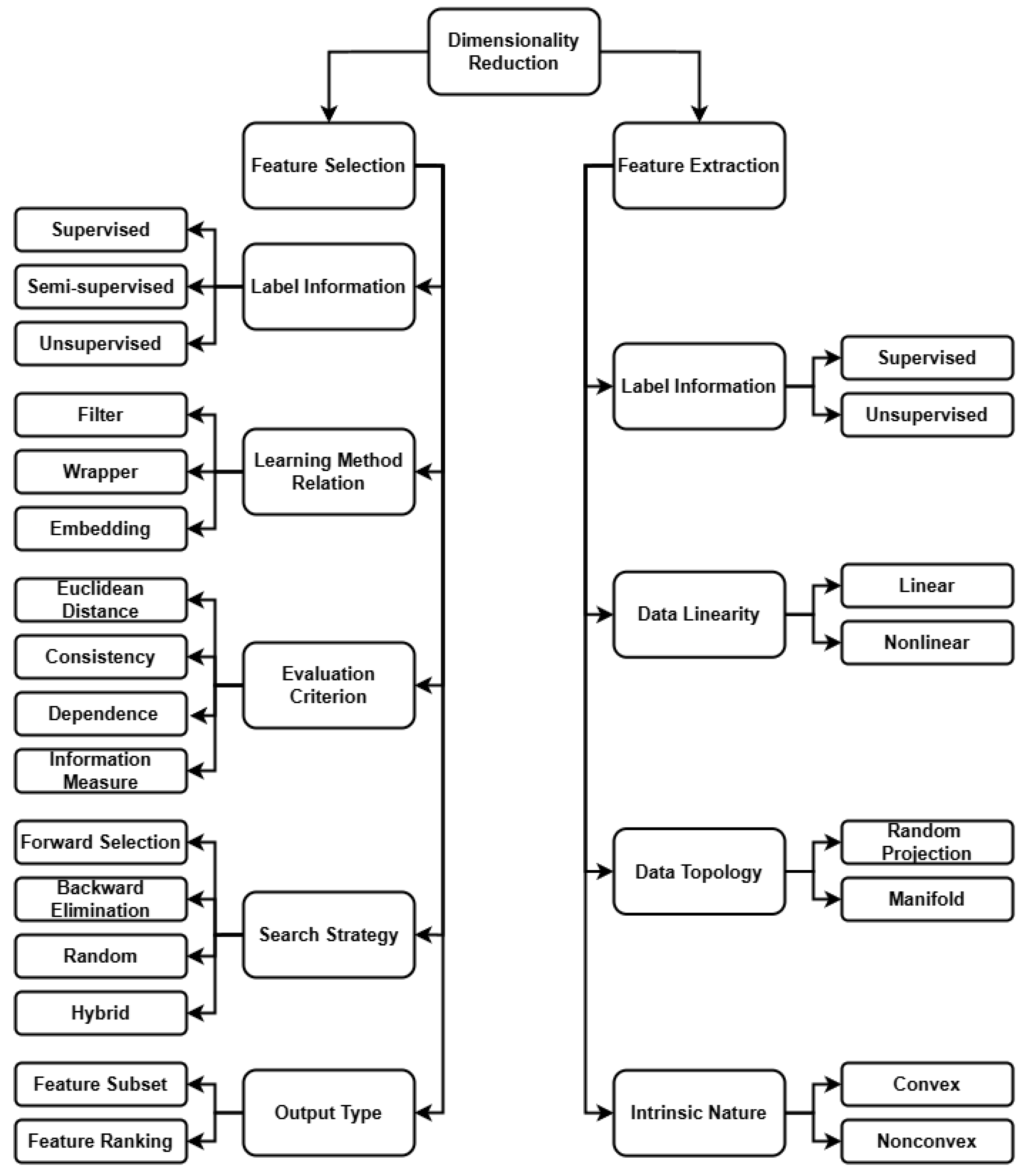
Feature selection is a critical component in developing robust and interpretable machine learning models. Conventional evaluation standards typically classify feature selection algorithms into three main categories: filter, wrapper, and embedded approaches. Each of these paradigms presents its own set of advantages and trade-offs. In the context of the present work, our primary objective is twofold: to maintain the freedom of choice regarding the final learning algorithm and to ensure that the feature selection process is computationally efficient.

While wrapper methods are known for their ability to evaluate feature subsets in direct relation to the performance of a learning algorithm, they are often computationally intensive (as documented in [17,23,24]). Given these constraints, our approach instead focuses on adapting a filter-based methodology. Traditional filter methods are prized for their speed and scalability; however, they typically overlook complex inter-dependencies between features. To address this limitation, an enhanced filter-based approach that partially accounts for inter-feature relationships is introduced. This modification enables the capture of interactions typically accessible only through the more computationally demanding wrapper methods.

Extending this line of reasoning, and in light of the capabilities presented by feature extraction approaches, it is theoretically viable to represent combinations of features through their intermediate representations. In doing so, one may apply feature selection not on the original variables, but instead on derived composite features that encapsulate higher-order interactions.

Consider, for instance, a dataset X of a given length. Our proposal envisions that this dataset can be approximately represented by a collection of n combinations, each comprising r features extracted from X. By employing such an interim representation, the modified filter-based selection method is afforded a broader and more nuanced feature space to explore—without incurring the high computational cost typically associated with wrapper techniques. This strategy is expected not only to significantly reduce the search time, but also to achieve performance metrics that are competitive with those of wrapper-based approaches.

In summation, the proposed framework offers a balanced solution by leveraging the computational efficiency of filter methods while simultaneously incorporating feature inter-dependencies to improve selection quality. This approach aims to allow for the rapid screening of a vast feature space, ensuring that the final selected set is both diverse and representative of the underlying data structure, thereby facilitating a more flexible and effective integration with subsequent learning algorithms.

The implementation of this approach relied on widely used Python libraries, including NumPy (1.23.5), Pandas (1.5.3), SciPy (1.11.3), Scikit-learn (1.2.1), and Py_FS (0.2.1). Among these, Scikit-learn and Py_FS played a particularly significant role in supporting the computational study discussed later in the article. Scikit-learn provided an extensive set of utility functions and facilitated the use of various filter-based feature selection and feature extraction techniques. Meanwhile, Py_FS was employed for its comprehensive suite of wrapper-based feature selection methods, which proved essential for the analysis.

3.2. Pitfalls

No truly foolproof approach exists; as such, it is to be expected that the proposed solution has its downsides, one of which may be self-evident even in a planning phase. This problem derives from its core concept, the use of interim features to represent combinations of the original ones, which is, in essence, a combinatorial problem.

As stated in [67], a combination refers to an unordered arrangement of a set of objects. Repetitions may or not be allowed. The number of r-combinations of a set with n distinct elements may be expressed as seen in Equation (1) [68].

$$C(n,r)\equiv {}_{n}C_r\equiv \left({\displaystyle \genfrac{}{}{0pt}{}{n}{r}}\right)\equiv {\displaystyle \frac{n!}{r!(n-r)!}}$$

(1)

By fixing a value for r (as 5 in this case) and then plotting the previous function, Figure 2 may be drawn:

As depicted in the plot (Figure 2), the number of combinations that can be created from a given group increases exponentially with the original sample size. For the proposed solution, it would become exponentially more expensive to use it for datasets with a large amount of features.

There are some ways to address this problem. One possibility would be to increase the number of features included in each combination group (r) in proportion to the increase in the total number of features (n). However, that would mean that for larger sets, each combination group would be equally broad, meaning that the effects of singular features and/or feature interactions would be greatly diluted.

A more permissible option would be to reduce the original feature set to a more manageable size. This can be accomplished by applying feature selection to the original set, and since the method should not be computationally expensive, a filter method is preferred.

3.3. Process

Given the proposed solution, a diagram of its intended progression is represented in Figure 3.

Starting from a full set, the solution reduces the number of redundant features. It accomplishes this by performing dependency analysis over the provided features and disposing of highly dependent ones, which are reduced to a single representative. It then selects the top features via a filter feature-selection method. This outputs a reduced set for which all feature combinations of length r are computed. Since the number of features n has been reduced, this operation is not as computationally expensive. The resulting list of feature groups is then used to create an entirely new dataset composed of features extracted from each of them. The new interim features dataset is subsequently used with a filter method (which may or not be the same as the one previously used) to select the best of them. Any of the selected interim features directly correspond to a set of possible solutions for selection, all of which have a length of r.

It should be taken into account that this process is adaptable since there are steps in which the algorithm to be used may be chosen as needed, and, in some cases, steps may be skipped. During the entire process, up to two different filter-based algorithms for feature selection may be chosen, as well as one for feature extraction. Additionally, if the dataset is not too large, a reduced representation may not be needed. A representation of this solution’s algorithm may be seen in Algorithm 1.

Algorithm 1: Proposed solution’s algorithm

The solution takes as input the dataset to be treated (D), its categorical features (if any) ($cf$), two filter-based feature selection methods (which may be the same) ($ff{s}_A,ff{s}_B$), the chosen feature extraction method ($fe$), the max value allowed for feature redundancy/dependency ($ma{x}_t$), the max feature set length to work with ($ma{x}_n$), and the target feature set length (r).

Starting from the full feature set, our approach addresses feature redundancy through dependency analysis to identify groups of highly dependent features. Specifically, features with a dependence value exceeding the threshold $ma{x}_t$ are classified as highly dependent. Each resulting group is then represented by a single feature that preserves the core information shared among its members. Although redundant features may contain subtle complementary signals, this consolidation strategy prioritizes unique, non-redundant features to maximize distinct information and minimize overlap. This initial dimensionality reduction step alleviates the computational complexity of subsequent analyses and reduces the risk of overfitting, thereby promoting the development of more robust predictive models.

Following this reduction, if the dataset’s number of dimensions still surpasses $ma{x}_n$, a filter-based feature selection method is employed to further identify and preserve the most promising features from the previously pruned set. This targeted selection ensures that only the most relevant features are carried forward, thereby streamlining the process.

Subsequently, the algorithm computes all possible feature combinations of a predetermined length, r, using the reduced feature set. These combinations are then used to generate a new dataset, wherein each derived feature corresponds to the extraction of each unique combination created using the chosen feature extraction method ($fe$). A second round of filter-based selection (potentially utilizing a different algorithm, $ff{s}_B$) is applied to this interim dataset to isolate its optimal features. The resultant features correspond directly to potential solutions, each comprising a feature set of length r. Going through its various steps returns the provided dataset reduced to its most relevant features (D).

4. Computational Study

In the following section, the results extracted from the proposed solution are presented and compared to those of other wrapper-based feature selection methods. These results and their meaning are then further discussed.

Taking into account the main problem referred to before, a test regarding the computation time necessary to create the interim features for all combinations of a dataset was carried out.

To illustratively validate the concern regarding the exponential growth in the number of feature combinations, an experiment was conducted. The length of combinations (r) was fixed at five, a value chosen to strike a balance between computational feasibility and representativeness of the underlying trend. This test was carried out using the proposed method without applying any preliminary feature reduction steps, thereby isolating the impact of the combinatorial explosion. The results may be observed in the plot depicted in Figure 4.

As expected, the exponential growth in potential combinations also significantly affects the temporal efficiency of the proposed algorithm, which only validates the importance of the first feature reduction steps proposed to counter it. Once that counter-measure was implemented, an experiment was designed to compare the performance of the proposed solution when compared to other feature selection methods.

To evaluate the effectiveness of our proposed solution, we compare its performance against nine established wrapper-based feature selection methods. This set of algorithms was chosen to provide a diverse and challenging benchmark, as wrapper methods are known to produce high-performing feature subsets. The selection represents a wide array of state-of-the-art metaheuristic strategies commonly used for optimization and feature selection. Furthermore, all comparative algorithms were implemented using the Py_FS package, which provides a standardized and fair framework for evaluating performance and computational cost. The chosen methods were:

1.

Binary Bat Algorithm (BBA)

2.

Cuckoo Search Algorithm (CSA)

3.

Equilibrium Optimizer (EO)

4.

Genetic Algorithm (GA)

5.

Gravitational Search Algorithm (GSA)

6.

Harmony Search (HS)

7.

Mayfly Algorithm (MA)

8.

Red Deer Algorithm (RDA)

9.

Whale Optimization Algorithm (WOA)

To conduct meaningful testing, a substantial number of data points are required. Consequently, thirty distinct datasets were utilized for both binary and multi-classification tasks, which may be reviewed in

Table 1. Characteristics of datasets used in the computational study.

Dataset	Source	Size	Features	Classification Type	Label Values
API security: Access behavior anomaly dataset	[69]	1699	9	Binary	2
Banking Dataset Classification	[70]	32,950	20	Binary	2
Bank Marketing	[71]	45,211	16	Binary	2
Breast Cancer Wisconsin (Original)	[72]	699	9	Binary	2
Churn Modeling	[73]	10,000	13	Binary	2
Taiwanese Bankruptcy Prediction	[74]	6819	95	Binary	2
CS:GO Round Winner Classification	[75]	122,410	96	Binary	2
Cure The Princess	[76]	2338	13	Binary	2
Depression	[77]	1429	22	Binary	2
EEG Eye State	[78]	14,980	14	Binary	2
Statlog (German Credit Data)	[79]	1000	20	Binary	2
GlaucomaM Dataset	[80]	196	62	Binary	2
Heart Failure Prediction Dataset	[81]	918	11	Binary	2
Home Loan Approval	[82]	614	11	Binary	2
IBM Attrition Dataset	[83]	1470	12	Binary	2
Ionosphere	[84]	351	34	Binary	2
MAGIC Gamma Telescope	[85]	19,020	10	Binary	2
Microcalcification Classification	[86]	11,183	6	Binary	2
Musk (Version 1)	[87]	476	168	Binary	2
Parkinsons	[88]	197	22	Binary	2
Pima Indians Diabetes Database	[89]	768	8	Binary	2
HTRU2	[90]	17,898	8	Binary	2
Rice Type Classification	[91]	18,185	10	Binary	2
Smoke Detection Dataset	[92]	62,630	12	Binary	2
Connectionist Bench (Sonar, Mines vs. Rocks)	[93]	208	60	Binary	2
Spambase	[94]	4601	57	Binary	2
Spotify Song Attributes	[95]	2017	16	Binary	2
Telescope Spectrum Gamma or Hadron	[96]	19,020	10	Binary	2
Titanic Dataset	[97]	891	10	Binary	2
Water Quality	[98]	7999	20	Binary	2
Personality classification Data: 16 Personalities	[99]	60,000	60	Multiclass	16
Customer Segmentation Classification	[100]	2627	9	Multiclass	4
Body Performance Data	[101]	13,393	11	Multiclass	4
COVID-19 Dataset	[102]	1,048,576	20	Multiclass	7
Dermatology	[103]	366	34	Multiclass	6
DnD Stats	[104]	10,000	9	Multiclass	9
Microsoft Malware Sample	[105]	1642	257	Multiclass	9
Glass Identification	[106]	214	9	Multiclass	7
Weight Lifting Exercise Dataset	[107]	19,622	152	Multiclass	5
HCV Data	[108]	615	12	Multiclass	5
Relationship Between Pain and MyersBriggs Personality Factors	[109]	97	18	Multiclass	4
League of Legends Stats: S12	[110]	232	9	Multiclass	6
Letter Recognition	[111]	20,000	16	Multiclass	26
Crystal System Properties for Li-ion Batteries	[112]	339	10	Multiclass	3
Clean Microsoft Malware Classification Challenge Dataset (BIG 2015)	[113]	10,868	68	Multiclass	9
Milk Quality Prediction	[114]	1059	7	Multiclass	3
Prediction of Music Genre	[115]	50,005	17	Multiclass	10
Orbit Classification for Prediction NASA	[116]	1748	11	Multiclass	6
Pokemon Unite Dataset	[117]	53	9	Multiclass	5
Poker Hand	[118]	1,025,010	10	Multiclass	10
Pump Sensor Dataset	[119]	220,320	52	Multiclass	3
Seeds	[120]	210	7	Multiclass	3
Sleep Health and Lifestyle Dataset	[121]	374	12	Multiclass	3
Soybean (Large)	[122]	307	35	Multiclass	19
Star Types Dataset	[123]	240	6	Multiclass	6
Vehicles Silhouettes	[124]	846	18	Multiclass	4
Video Games Rating by ’ESRB’	[125]	1895	33	Multiclass	4
Vowel Recognition-Deterding Data	[126]	990	10	Multiclass	11
Wine Quality	[127]	4898	11	Multiclass	11
Zoo	[128]	101	16	Multiclass	7

.

The framework was designed as follows:

1.

All datasets are pre-processed in order to guarantee no missing rows and numerical features are standardized

2.

A cycle iterates over each combination of existing datasets and methods. In each step, the following occurs (seen in Algorithm 2):

(a)

The dataset is read.

(b)

For datasets exceeding 10,000 rows, a stratified sample of 10,000 instances was used to reduce the computational load while preserving the original class distribution. This approach minimizes the loss of informative patterns and ensures that the sampled subset remains representative of the full dataset.

(c)

Its categorical features are encoded by using target encoding (these features are identified beforehand).

(d)

This dataset is used with the current method, which iterates over the proposed solution and the remaining methods (these use 30 agents, and a max of 50 iterations, as these are the chosen defaults of Py_FS) to find a solution set.

(e)

Given the solution set arrived at by the feature selection method, the best sets of features found for target lengths [2–5] are retrieved.

(f)

For each of the target lengths, the best set found (if any) is used to train a default random forest classifier.

(g)

Performance metrics are then retrieved from the trained classifier.

3.

These metrics are then saved while being associated with the feature selection method and dataset involved in the current step.

Algorithm 2: Testing cycle’s algorithm

For this test, PCA was the chosen extraction method. This was the case since PCA has been extensively utilized in various experimental settings, particularly in the fields of biometrics, image processing, and fault detection, due to its effectiveness in feature extraction. Some notable examples are its usage in the realm of iris and face recognition [129,130,131]. However, one limitation of PCA is that it may fail to capture complex non-linear structures that are often present in real-world datasets. To address this limitation, the approach chosen was to use Random Fourier Features (RFF). RFF approximates non-linear kernel methods (specifically those based on shift-invariant kernels like the Radial Basis Function) by mapping the input data into a randomized low-dimensional feature space where linear techniques can then be applied [132].

Additionally, Mutual Information (MI) was employed as the filter-based feature selection algorithm for this experiment. This choice was motivated by several factors. First, MI has consistently demonstrated effectiveness across a wide range of feature selection scenarios, making it a robust and well-validated method [133,134]. Second, MI is computationally efficient, which aligns well with the broader objective of this study to maintain reasonable resource usage across large-scale evaluations. Finally, unlike correlation metrics, such as Pearson’s or Kendall’s coefficient, MI can capture both non-linear and non-monotonic dependencies between features and the target variable [135]. This makes it particularly suitable for complex datasets where relationships among variables may not be simplistic.

Prior to applying any feature selection methods, all datasets used for testing underwent a standardized pre-processing pipeline. Rows with missing values were removed to ensure consistent input for downstream processing (although these were few in number due to this being a factor during dataset selection). Numerical features were standardized (using Z-score scaling) to ensure comparability across dimensions and to prevent features with larger magnitudes from dominating others.

Categorical features were encoded within the evaluation loop itself, using target encoding with smoothing to avoid introducing target leakage. This design was adopted in order to allow for easy substitution of encoding strategies if needed. Notably, one-hot encoding was avoided, as it would have prohibitively inflated the dimensionality of the feature space.

It is important to note that the pre-processing step was applied uniformly across all methods. Based on empirical observations during testing, the time spent on pre-processing was consistently negligible. While not formally benchmarked, this suggests that pre-processing does not materially affect the relative performance comparisons reported.

In this study, all feature selection methods and the downstream random forest classifier were evaluated using their default hyper-parameters. This decision was guided by considerations of fairness, computational feasibility, and reproducibility. Using default settings ensured a consistent baseline across all methods, allowing performance differences to reflect algorithmic behavior rather than hyperparameter tuning. Moreover, auto-tuning would have introduced a prohibitive computational overhead. Given the scale of the study—ten optimizers (the proposed approach plus nine wrapper approaches), sixty datasets, and multiple feature set sizes—exploring additional hyperparameter combinations would have multiplied the runtime significantly, rendering the analysis impractical.

Finally, default configurations reflect typical usage scenarios, making the results more accessible and easier to replicate. The chosen defaults are generally sensible values that offer a good balance between performance and abstraction of usage. While future work may explore optimized configurations, the use of defaults provided a balanced and efficient framework for large-scale comparison.

Due to the design of the wrapper-based feature selection methods (where the best feature subsets are selected independently of the target subset length), it is possible that fewer than thirty valid data points were obtained for certain target lengths r. While this does not pose a methodological issue, it limits the extent to which these subsets can be assumed to follow a normal distribution under the central limit theorem [136]. To address this, all wrapper-based methods were later aggregated into a single group during the statistical analysis, thereby ensuring a sufficient sample size and enabling a more reliable approximation to normality for comparative purposes.

The metrics used to measure the performance of the fitted classifiers were:

• Weighted Precision—obtained by calculating the precision for each involved label, and finding their average weighted by the number of true instances for each label.
• Weighted Recall—obtained by calculating the recall for each involved label, and finding their average weighted by the number of true instances for each label.
• Weighted FBeta—obtained by calculating the fbeta score for each involved label, and finding their average weighted by the number of true instances for each label.
• Time—obtained by measuring the elapsed time during the testing process

The collected results were used to plot the graphs seen in Figure 5, Figure 6, Figure 7, Figure 8, Figure 9, Figure 10, Figure 11 and Figure 12.

To further explore the collected results, and statistically test them, all data points were then divided into two groups “Proposed” and “Other”, which took into account the proposed method (PM) data points and all other data points, respectively. Thus, the central limit theorem was respected in both groups, meaning both should converge to a standard normal distribution. By plotting these new data groups according to the metrics mentioned earlier, Figure 13, Figure 14, Figure 15, Figure 16, Figure 17, Figure 18, Figure 19 and Figure 20 are produced. Specifically, in the case of the points relating to the elapsed time, the data regarding MA and RDA were excluded so as to not negatively impact the other approaches.

To statistically validate the observed performance differences between the proposed method and the baseline approaches, we applied a combination of Welch’s two-tailed t-tests and Generalized Least Squares (GLS) regression models. Welch’s t-test is appropriate for comparing two groups with potentially unequal variances and sample sizes, which suits our experimental setting where the number of valid data points varies across methods and feature set sizes. GLS modeling further allowed us to estimate the effect of the independent variables (specifically, the feature set length and method group) on each performance metric while controlling for task type (binary or multi-class classification). This dual approach ensures that the results are statistically sound and robust towards the structure and distribution of data.

The full summary statistics for the GLS models are presented in

Table 2. GLS statistics for weighted precision in binary classification.

Dep. Variable:	${\mathit{R}}^2$	Adj. ${\mathit{R}}^2$	F	$\mathbf{Pr}\left(\mathit{F}\right)$	$log\mathit{L}$
Weighted Precision	0.034	0.029	5.128	0.00165	494.12
	$\widehat{\mathit{\beta }}$	$\mathbf{SE}$	$\mathit{z}$	$\mathbf{Pr}(>|\mathit{z}\left|\right)$	[0.025	0.975]
Intercept	0.9327	0.017	54.549	0.000	0.899	0.966
CombLength	−0.0017	0.004	−0.398	0.691	−0.010	0.007
Group[T.Proposed]	−0.1142	0.044	−2.615	0.009	−0.200	−0.029
CombLength:Group[T.Proposed]	0.0195	0.011	1.756	0.079	−0.002	0.041

,

Table 3. GLS statistics for weighted precision in multi-class classification.

Dep. Variable:	${\mathit{R}}^2$	Adj. ${\mathit{R}}^2$	F	$\mathbf{Pr}\left(\mathit{F}\right)$	$log\mathit{L}$
Weighted Precision	0.028	0.023	4.282	0.00527	139.90
	$\widehat{\mathit{\beta }}$	$\mathbf{SE}$	$\mathit{z}$	$\mathbf{Pr}(>|\mathit{z}\left|\right)$	[0.025	0.975]
Intercept	0.8126	0.030	27.330	0.000	0.754	0.871
CombLength	0.0026	0.008	0.339	0.735	−0.012	0.018
Group[T.Proposed]	−0.1668	0.077	−2.180	0.029	−0.317	−0.017
CombLength:Group[T.Proposed]	0.0267	0.020	1.321	0.187	−0.013	0.066

,

Table 4. GLS statistics for weighted recall in binary classification.

Dep. Variable:	${\mathit{R}}^2$	Adj. ${\mathit{R}}^2$	F	$\mathbf{Pr}\left(\mathit{F}\right)$	$log\mathit{L}$
Weighted Recall	0.034	0.029	5.073	0.00178	511.84
	$\widehat{\mathit{\beta }}$	$\mathbf{SE}$	$\mathit{z}$	$\mathbf{Pr}(>|\mathit{z}\left|\right)$	[0.025	0.975]
Intercept	0.9336	0.017	56.180	0.000	0.901	0.966
CombLength	−0.0014	0.004	−0.344	0.731	−0.010	0.007
Group[T.Proposed]	−0.1117	0.043	−2.605	0.009	−0.196	−0.028
CombLength:Group[T.Proposed]	0.0193	0.011	1.767	0.077	−0.002	0.041

,

Table 5. GLS statistics for weighted recall in multi-class classification.

Dep. Variable:	${\mathit{R}}^2$	Adj. ${\mathit{R}}^2$	F	$\mathbf{Pr}\left(\mathit{F}\right)$	$log\mathit{L}$
Weighted Recall	0.046	0.042	6.787	0.000166	134.43
	$\widehat{\mathit{\beta }}$	$\mathbf{SE}$	$\mathit{z}$	$\mathbf{Pr}(>|\mathit{z}\left|\right)$	[0.025	0.975]
Intercept	0.8035	0.030	26.553	0.000	0.744	0.863
CombLength	0.0038	0.008	0.490	0.624	−0.011	0.019
Group[T.Proposed]	−0.2272	0.080	−2.834	0.005	−0.384	−0.070
CombLength:Group[T.Proposed]	0.0381	0.021	1.819	0.069	−0.003	0.079

,

Table 6. GLS statistics for weighted F-beta in binary classification.

Dep. Variable:	${\mathit{R}}^2$	Adj. ${\mathit{R}}^2$	F	$\mathbf{Pr}\left(\mathit{F}\right)$	$log\mathit{L}$
Weighted F-beta	0.036	0.031	5.329	0.00125	496.06
	$\widehat{\mathit{\beta }}$	$\mathbf{SE}$	$\mathit{z}$	$\mathbf{Pr}(>|\mathit{z}\left|\right)$	[0.025	0.975]
Intercept	0.9327	0.017	54.692	0.000	0.899	0.966
CombLength	−0.0017	0.004	−0.404	0.686	−0.010	0.007
Group[T.Proposed]	−0.1184	0.044	−2.697	0.007	−0.205	−0.032
CombLength:Group[T.Proposed]	0.0205	0.011	1.838	0.066	−0.001	0.042

,

Table 7. GLS statistics for weighted F-beta in multi-class classification.

Dep. Variable:	${\mathit{R}}^2$	Adj. ${\mathit{R}}^2$	F	$\mathbf{Pr}\left(\mathit{F}\right)$	$log\mathit{L}$
Weighted F-beta	0.054	0.050	7.600	5.37 × 10−5	109.07
	$\widehat{\mathit{\beta }}$	$\mathbf{SE}$	$\mathit{z}$	$\mathbf{Pr}(>|\mathit{z}\left|\right)$	[0.025	0.975]
Intercept	0.7937	0.032	25.172	0.000	0.732	0.855
CombLength	0.0044	0.008	0.544	0.586	−0.011	0.020
Group[T.Proposed]	−0.2599	0.086	−3.012	0.003	−0.429	−0.091
CombLength:Group[T.Proposed]	0.0440	0.022	1.962	0.050	5.33 × 10−5	0.088

,

Table 8. GLS statistics for elapsed time in binary classification.

Dep. Variable:	${\mathit{R}}^2$	Adj. ${\mathit{R}}^2$	F	$\mathbf{Pr}\left(\mathit{F}\right)$	$log\mathit{L}$
Elapsed Time	0.119	0.114	98.98	4.80 × 10−51	−2758.5
	$\widehat{\mathit{\beta }}$	$\mathbf{SE}$	$\mathit{z}$	$\mathbf{Pr}(>|\mathit{z}\left|\right)$	[0.025	0.975]
Intercept	27.3267	7.354	3.716	0.000	12.913	41.740
CombLength	3.5696	2.003	1.782	0.075	−0.356	7.495
Group[T.Proposed]	−33.3802	7.859	−4.247	0.000	−48.784	−17.976
CombLength:Group[T.Proposed]	0.1718	2.253	0.076	0.939	−4.244	4.588

and

Table 9. GLS statistics for elapsed time in multi-class classification.

Dep. Variable:	${\mathit{R}}^2$	Adj. ${\mathit{R}}^2$	F	$\mathbf{Pr}\left(\mathit{F}\right)$	$log\mathit{L}$
Elapsed Time	0.052	0.047	46.41	9.49 ×10−27	−2846.2
	$\widehat{\mathit{\beta }}$	$\mathbf{SE}$	$\mathit{z}$	$\mathbf{Pr}(>|\mathit{z}\left|\right)$	[0.025	0.975]
Intercept	18.5391	7.198	2.575	0.010	4.431	32.648
CombLength	2.8740	2.049	1.402	0.161	−1.143	6.891
Group[T.Proposed]	−24.4107	7.656	−3.189	0.001	−39.416	−9.406
CombLength:Group[T.Proposed]	0.7652	2.268	0.337	0.736	−3.679	5.210

. The results from the Welch’s t-tests (reported in

Table 10. Results of Welch’s two-sided t-test when comparing the proposed approach to others.

Sample 1	Sample 2	Dep. Variable	Task Type	Comb. Length	z	p-Value	[0.025	0.975]
Proposed	Other	Weighted Precision	Binary	2	−3.339137	0.001847	−0.153447	−0.037696
				3	−1.229258	0.225446	−0.080478	0.019488
				4	−1.794048	0.080092	−0.077424	0.004564
				5	−1.180861	0.244622	−0.065889	0.017288
			Multiclass	2	−2.467175	0.017900	−0.214318	−0.021371
				3	−1.940488	0.059348	−0.184331	0.003732
				4	−1.270337	0.211616	−0.134787	0.030829
				5	−0.871282	0.389142	−0.122213	0.048689
		Weighted Recall	Binary	2	−3.352493	0.001792	−0.152162	−0.037641
				3	−1.142918	0.259045	−0.074779	0.020624
				4	−1.785279	0.081473	−0.074297	0.004553
				5	−1.201707	0.236575	−0.064053	0.016289
			Multiclass	2	−3.078687	0.003750	−0.261752	−0.054278
				3	−2.480135	0.017450	−0.209854	−0.021396
				4	−1.474974	0.148269	−0.142144	0.022265
				5	−1.078255	0.287842	−0.130507	0.039834
		Weighted F−beta	Binary	2	−3.435131	0.001418	−0.157873	−0.040860
				3	−1.203859	0.234931	−0.078563	0.019780
				4	−1.826457	0.074973	−0.077599	0.003880
				5	−1.186296	0.242495	−0.065528	0.017054
			Multiclass	2	−3.217494	0.002604	−0.293295	−0.066871
				3	−2.674836	0.010816	−0.226520	−0.031499
				4	−1.579989	0.122288	−0.153480	0.018890
				5	−1.131926	0.264919	−0.139474	0.039485
		Elapsed Time	Binary	2	−6.666344	3.211123 × 10−9	−39.615647	−21.398280
				3	−8.718218	2.736172 × 10−14	−42.999578	−27.075706
				4	−8.527798	4.795209 × 10−14	−43.566578	−27.150573
				5	−5.398764	3.330228 × 10−7	−41.028112	−19.013613
			Multiclass	2	−5.158019	1.498194 × 10−6	−28.779376	−12.772675
				3	−5.820468	5.658046 × 10−8	−32.897706	−16.188448
				4	−5.185412	8.925830 × 10−7	−31.272672	−13.989275
				5	−3.204767	1.677736 × 10−3	−30.575765	−7.242982

) confirm that the differences observed across several key metrics are statistically significant, particularly with respect to computational time and performance trends as the feature set length increases.

For reference, the hardware used to carry out these tests was a setup consisting of an MSI X370 mainboard, an AMD Ryzen 5 5600G CPU with a max clock speed of 4.4 GHz, a NVIDIA GeForce RTX 3070 GPU and 36 GBytes of DDR4 RAM running at 16 MHz.

Discussion

In Figure 5, Figure 6, Figure 7, Figure 8, Figure 9, Figure 10, Figure 11, Figure 12, Figure 13, Figure 14, Figure 15, Figure 16, Figure 17, Figure 18, Figure 19 and Figure 20, some outliers can be observed; as in any experiment, some amount of variability is expected, but some hypothesis should be put forward. Through observation of the presented boxplots, it is possible to see that most outliers are detected in the wrapper methods put forward to compare to the proposed solution. These outliers may result from various factors, either individually or in combination. Firstly, as was explained previously, these algorithms suffer a degree of randomness due to their design—it is possible that the initial solutions generated for these cases were simply extreme when compared to the norm. A second hypothesis could be that some of the datasets used in this experiment are not a good fit with these algorithms’ approach, meaning they inherently present a bad performance when compared to the average case. Observing the plots presented in Figure 17 and Figure 18, it can be discerned that the wrapper approaches seem to present some outliers referring to combination lengths of 2 under binary classification. This may be caused due to the datasets provided for testing in this context not being well represented by a small amount of features in most cases according to these methods’ approach.

In Figure 5, Figure 6, Figure 7, Figure 8, Figure 9 and Figure 10, the most clear trend present across the various plots is the improvement in performance of the PM as the length of the target feature set (combination_len) increases. The same trend seems to be visible in other methods such as EO and WOA, although it is less pronounced and more subtle. Through observation, it seems clear that PM lacks performance in smaller target set lengths; however, it rapidly catches the other methods with respect to performance when allowed to work with greater ones, even competing with most other feature selection methods. The loss in performance between binary and multi-classification tasks should also be pointed out. This decrease in performance is expected as multi-class classification is a distinctly more difficult task when compared to binary classification.

In Figure 11 and Figure 12, it is possible to observe the elapsed time distribution for each feature-selection method. It is important to note that due to how these other methods work (i.e., an agent-based architecture that has multiple agents search a solution space), a correction is taken into account regarding the max number of iterations and agents available for each one. This means that if, for example, the BBA method took 20,000 s in each of its tasks, the correct time to be compared to the PM would be as follows: 20,000 s/30 agents/50 iterations. This correction is applied to each data point collected from methods other than the PM. Despite that, as is observable, the PM still seemingly outperforms the other methods in all cases.

Turning to the results pertaining to the two grouped division depicted in Figure 13, Figure 14, Figure 15, Figure 16, Figure 17, Figure 18, Figure 19 and Figure 20. The overall conclusion from observing these plots matches those from the previous steps where other approaches were separate. The direct relation between the PM’s performance and the length of the target feature is still apparent. A clear difference is visible between the PM and other solutions; however, the more the target set grows the more both groups approach each other, while maintaining a significant disparity in computational time.

These inferences may be further examined by resorting to the coefficients presented in Table 2, Table 3, Table 4, Table 5, Table 6, Table 7, Table 8 and Table 9.

By analyzing the coefficients present in the GLS models represented in these tables, some conclusions can be drawn. Firstly, it is possible to reject the null hypothesis associated with the F-statistic for each GLS model—that is, the hypothesis that the independent variables and their interactions do not affect the dependent variable. This rejection is supported by the very low p-values (all below a significance threshold of $\alpha =0.05$, corresponding to a 95% confidence level). It is important to note, however, that the primary objective of these GLS models is not to achieve strong predictive power, but rather to explore and analyze the relationships between the independent variables and the dependent variable. Despite low R² values, the statistical significance of the models ensures that the identified relationships are meaningful within the context of the analysis. Additionally, any conclusions derived from these models will later be compared to other analysis approaches, such as graphical analysis and two-tailed t-tests, to reinforce the robustness and consistency of the findings.

Focusing on the different dependent variables, some conclusions may be reached. Through comparison of coefficients relative to Group[T.Proposed] for precision, recall, and f-beta, it is clear that PM does not readily match the performance achieved by other approaches. This conclusion is very significant ($\alpha$ = 0.05 ≥p value) for all the cases presented. Counteracting the last point, the effect of the target feature set length (combination length) appears to impact the various dependent variables positively specifically for PM. This conclusion approaches significance for all cases except one, which means it is significant ($\alpha$ = 0.1 ≥ p value). The exception occurs for weighted precision in the case of multi-classification in which the relevant p-value is equal to 0.187, which means the calculated coefficient is only relevant for approximately 80% of cases.

The observations exposed above are largely reiterated when analyzing the results obtained for the t-tests across the two groups (Table 10). Taking into account weighted precision, weighted recall, and weighted F-beta, it is possible to conclude that the difference between the two groups, seems to become smaller and less relevant the more the combination length increases. This conclusion is reached since the test statistic (z) for these cases tends to decrease in absolute value, which denotes a smaller difference, and the p-value on the other hand tends to increase, which allows for a stronger assurance relative to the methods null hypothesis; in this case $H_0:\mu 1=\mu 2$, meaning the difference between the two groups becomes less clear.

These conclusions are consistent with the behavior observed in Figure 13, Figure 14, Figure 15, Figure 16, Figure 17 and Figure 18.

Concerning the elapsed time, in all cases, it is apparent that the PM is significantly faster than other solutions. This is observable through the coefficient values present for Group[T.Proposed]. This conclusion stands as strongly significant both for binary and multi-class classification, since $\alpha$ = 0.05 ≥ p value, as observed in Table 8 and Table 9. Additionally, the target feature set length appears to have little impact in regards to the PM, as may be observed through the confidence values for CombLength:Group[T.Proposed] on those same tables, as well as their p-values, which do not allow for a reasonable significance level. Another conclusion one may make, although secondary, is that the group composed of other approaches is more affected by an increase in the elapsed time caused by an increase in the target feature set length; this may be interpreted through the difference between the value and the significance seen between the coefficients for CombLength and CombLength:Group[T.Proposed] in both cases.

The same conclusion may be reached through consultation of Table 10, in which, no matter the combination length or task type involved, there appears to be a clear difference between the two groups. This is denoted by the very low p-values and the negative values presented for the test statistic (z), which indicate an advantage for the proposed method regarding computational speed. This significant difference may be further observed by checking the confidence intervals involved in this dependent variable’s case.

These conclusions are, as above, consistent with the behavior demonstrated in Figure 19 and Figure 20.

Due to computational cost constraints, the method was not evaluated on datasets containing thousands of features. However, an analysis of descriptive statistics from datasets with 90 or more features indicates that the proposed approach remains competitive even at higher dimensionalities. Specifically, the method achieves a mean elapsed time of 10.6 s with a standard deviation of 12 s for this subset. This outperforms the average computational time observed across all datasets for other approaches, which exhibit a mean of 34.5 s and a standard deviation of 45.6 s. Although the average processing time for datasets with over 90 features is higher compared to those with fewer features (4.6 s mean, 6.3 s standard deviation), the method still demonstrates efficient performance, which is expected to stabilize further due to the previously discussed countermeasures.

5. Conclusions

Machine learning has been under a state of constant evolution in recent years—a good part of this may be attributed to great amounts of training data associated with better infrastructure [1]. However, certain fields and applications do not have this same degree of data availability, be it due to monetary costs, temporal costs, or simple scarcity of data relating to the subject matter [4]. This makes it especially important to know the most relevant features for a given task, as they have an associated cost. For this purpose, and to improve over use of wrapper or filter-based feature selection techniques, an approach using feature extraction to represent interim combinations of features from the original dataset was proposed.

This approach aims to counter downfalls present in regular feature selection alternatives [22], namely, temporal cost in the case of wrapper methods, and disregard for feature interaction in the case of filter methods. The method operates by generating interim representations of feature combinations, which are then scored and selected using lightweight filter metrics. This structure is designed to mitigate the primary limitations of classical approaches while remaining adaptable across a variety of contexts.

The computational study demonstrated that the proposed method offers notable improvements in efficiency, particularly when selecting medium-length feature subsets. In these cases, its predictive performance was found to be comparable to that of several state-of-the-art wrapper-based methods, while requiring significantly less time. Statistical analyses using GLS models and Welch’s t-tests reinforced these observations, highlighting consistent trends across dataset types.

Designed with modularity in mind, the method allows for user-defined configurations of feature extractors and filter strategies, making it highly adaptable to different modeling scenarios. These characteristics, combined with its empirical performance, suggest that the method can serve as a practical tool for feature selection in constrained environments.

5.1. Limitations

Despite its strengths, the proposed method is not without limitations. Chief among them is the combinatorial growth in the number of feature groups as the dimensionality of the dataset increases. While mitigated by initial redundant feature filtering and limiting the feature pool (e.g., max_n = 20), this complexity remains a core constraint of the approach.

Another important limitation relates to dataset suitability. The method performs best when the target feature set size is of moderate size and when the dataset has sufficient structure for shallow transformations to capture informative patterns. It may be less effective in scenarios where:

• Non-linear or hierarchical interactions dominate the data,
• Very large numbers of features ($n\gg$ $\mathrm{10,000}$) are present without the possibility of effective pre-filtering;
• Real-time constraints require ultra-low latency beyond what even this method can accommodate;
• The application demands deeply contextual or sequential understanding of features (e.g., natural language or temporal series);
• The dataset is naturally very sparce, or there are a very low number of samples (in these cases, approaches such as meta-learning or few-shot learning would be better suited).

• Furthermore, the use of default hyper-parameters in the experimental setup, while beneficial for reproducibility, may limit the method’s relative performance under different modeling configurations.

5.2. Future Work

Several promising research directions can be pursued to further refine and expand the proposed method.

First, to address the issue of combinatorial complexity, an iterative pruning strategy could be explored. A potential strategy would be to iteratively create interim feature sets with only one less element than the total available feature set, until reaching the desired length. As an example, the amount of combinations involved in a group of 100 elements for a sample size of 5 is 75,287,520; however, the amount of interim feature sets needed by iteratively eliminating the worse-performing ones is merely 5035. This happens since, in each step, the amount of interim feature sets created is equal to the length of the available feature set. The total amount of interim sets created is equal to the sum of all elements between the maximum feature set length and the target feature length, as may be seen in Equation (2).

$${\displaystyle \frac{n!}{(n-1)!(n-(n-1\left)\right)!}}={\displaystyle \frac{n\times (n-1)!}{(n-1)!}}=n$$

(2)

This process largely decreases the amount of interim sets needed, which may contribute to better performance [69].

Second, the integration of additional feature extraction techniques could further increase the robustness of the proposed method. A systematic comparison of such extractors under different data contexts would help establish optimal configurations for diverse application areas.

Third, the method could include an AutoML pipeline, enabling automated exploration of filter criteria, transformation methods, as well as combination lengths. This would enhance usability for non-expert users and reduce the need for manual tuning.

Lastly, domain-specific applications represent a compelling area for deployment. The proposed algorithm encompasses several potential use cases for its application. One of these use cases is in bioinformatics, where datasets often contain a vast number of features, such as gene expression levels. Feature selection often leads to better results in such cases as is presented by Kasikci in [137]. A different application of this method that may make use of its biggest advantage, its computational efficiency, is in settings where a faster (but not immediate) decision is needed, such as in medical diagnostics, and similarly to the previous case, medicine is no stranger to the use of feature selection be it due to excessive dimension or costs [4].

References

1. Roh, Y.; Heo, G.; Whang, S.E. A survey on data collection for machine learning: A big data-ai integration perspective. IEEE Trans. Knowl. Data Eng. 2019, 33, 1328–1347. [Google Scholar] [CrossRef]
2. Ramesh, A.; Dhariwal, P.; Nichol, A.; Chu, C.; Chen, M. Hierarchical text-conditional image generation with clip latents. arXiv 2022, arXiv:2204.06125. [Google Scholar] [CrossRef]
3. Achiam, J.; Adler, S.; Agarwal, S.; Ahmad, L.; Akkaya, I.; Aleman, F.L.; Almeida, D.; Altenschmidt, J.; Altman, S.; Anadkat, S.; et al. Gpt-4 technical report. arXiv 2023, arXiv:2303.08774. [Google Scholar] [CrossRef]
4. Ko, J.; Baldassano, S.N.; Loh, P.L.; Kording, K.; Litt, B.; Issadore, D. Machine learning to detect signatures of disease in liquid biopsies–a user’s guide. Lab Chip 2018, 18, 395–405. [Google Scholar] [CrossRef] [PubMed]
5. Esmeli, R.; Bader-El-Den, M.; Abdullahi, H. Session similarity based approach for alleviating cold-start session problem in e-commerce for Top-N recommendations. In Proceedings of the 12th International Joint Conference on Knowledge Discovery, Budapest, Hungary, 2–4 November 2020; pp. 179–186. [Google Scholar]
6. Tabatabaei, S.A.; Hoogendoorn, M.; van Halteren, A. Narrowing reinforcement learning: Overcoming the cold start problem for personalized health interventions. In Proceedings of the PRIMA 2018: Principles and Practice of Multi-Agent Systems: 21st International Conference, Tokyo, Japan, 29 October–2 November 2018; pp. 312–327. [Google Scholar]
7. Qiao, S.; Liu, C.; Shen, W.; Yuille, A.L. Few-shot image recognition by predicting parameters from activations. In Proceedings of the IEEE Conference on Computer Vision and Pattern Recognition, Salt Lake City, UT, USA, 18–23 June 2018; pp. 7229–7238. [Google Scholar]
8. McShane, L.; Pancer, E.; Poole, M.; Deng, Q. Emoji, playfulness, and brand engagement on twitter. J. Interact. Mark. 2021, 53, 96–110. [Google Scholar] [CrossRef]
9. Del Vecchio, P.; Secundo, G.; Garzoni, A. Phygital technologies and environments for breakthrough innovation in customers’ and citizens’ journey. A critical literature review and future agenda. Technol. Forecast. Soc. Change 2023, 189, 122342. [Google Scholar] [CrossRef]
10. Birjali, M.; Kasri, M.; Beni-Hssane, A. A comprehensive survey on sentiment analysis: Approaches, challenges and trends. Knowl.-Based Syst. 2021, 226, 107134. [Google Scholar] [CrossRef]
11. Gandhi, A.; Adhvaryu, K.; Poria, S.; Cambria, E.; Hussain, A. Multimodal sentiment analysis: A systematic review of history, datasets, multimodal fusion methods, applications, challenges and future directions. Inf. Fusion 2023, 91, 424–444. [Google Scholar] [CrossRef]
12. Talbi, E.G. Hybrid Metaheuristics; Springer: Berlin/Heidelberg, Germany, 2013; Volume 166. [Google Scholar]
13. Berisha, V.; Krantsevich, C.; Hahn, P.R.; Hahn, S.; Dasarathy, G.; Turaga, P.; Liss, J. Digital medicine and the curse of dimensionality. NPJ Digit. Med. 2021, 4, 153. [Google Scholar] [CrossRef]
14. Anowar, F.; Sadaoui, S.; Selim, B. Conceptual and empirical comparison of dimensionality reduction algorithms (PCA, KPCA, LDA, MDS, SVD, LLE, ISOMAP, LE, ICA, t-SNE). Comput. Sci. Rev. 2021, 40, 100378. [Google Scholar] [CrossRef]
15. Dhal, P.; Azad, C. A comprehensive survey on feature selection in the various fields of machine learning. Appl. Intell. 2022, 52, 4543–4581. [Google Scholar] [CrossRef]
16. Cai, J.; Luo, J.; Wang, S.; Yang, S. Feature selection in machine learning: A new perspective. Neurocomputing 2018, 300, 70–79. [Google Scholar] [CrossRef]
17. Pudjihartono, N.; Fadason, T.; Kempa-Liehr, A.W.; O’Sullivan, J.M. A review of feature selection methods for machine learning-based disease risk prediction. Front. Bioinform. 2022, 2, 927312. [Google Scholar] [CrossRef] [PubMed]
18. Miao, J.; Niu, L. A survey on feature selection. Procedia Comput. Sci. 2016, 91, 919–926. [Google Scholar] [CrossRef]
19. Dokeroglu, T.; Deniz, A.; Kiziloz, H.E. A comprehensive survey on recent metaheuristics for feature selection. Neurocomputing 2022, 494, 269–296. [Google Scholar] [CrossRef]
20. Al-Tashi, Q.; Kadir, S.J.A.; Rais, H.M.; Mirjalili, S.; Alhussian, H. Binary optimization using hybrid grey wolf optimization for feature selection. IEEE Access 2019, 7, 39496–39508. [Google Scholar] [CrossRef]
21. Bhattacharyya, T.; Chatterjee, B.; Singh, P.K.; Yoon, J.H.; Geem, Z.W.; Sarkar, R. Mayfly in harmony: A new hybrid meta-heuristic feature selection algorithm. IEEE Access 2020, 8, 195929–195945. [Google Scholar] [CrossRef]
22. Bellotti, T.; Nouretdinov, I.; Yang, M.; Gammerman, A. Feature selection. In Balasubramanian, Conformal Prediction for Reliable Machine Learning: Theory, Adaptations and Applications; Ho, V.N., Vovk, S.-S., Eds.; Elsevier: Amsterdam, The Netherlands, 2014; pp. 116–130. [Google Scholar]
23. Verhaeghe, J.; Donckt, J.V.D.; Ongenae, F.; Hoecke, S.V. Powershap: A power-full shapley feature selection method. In Lecture Notes in Computer Science; Springer: Cham, Switzerland, 2023; pp. 71–87. [Google Scholar] [CrossRef]
24. Alyasiri, O.M.; Cheah, Y.; Abasi, A.K.; Al-Janabi, O.M. Wrapper and hybrid feature selection methods using metaheuristic algorithms for english text classification: A systematic review. IEEE Access 2022, 10, 39833–39852. [Google Scholar] [CrossRef]
25. Hamla, H.; Ghanem, K. Comparative study of embedded feature selection methods on microarray data. In Proceedings of the Artificial Intelligence Applications and Innovations: 17th IFIP WG 12.5 International Conference, AIAI 2021, Hersonissos, Crete, Greece, 25–27 June 2021; pp. 69–77. [Google Scholar]
26. Ruiz, I.L.; Gómez-Nieto, M.Á. Building Highly Reliable Quantitative Structure–Activity Relationship Classification Models Using the Rivality Index Neighborhood Algorithm with Feature Selection. J. Chem. Inf. Model. 2020, 60, 133–151. [Google Scholar] [CrossRef]
27. Van Der Maaten, L.; Postma, E.; Van den Herik, J. Dimensionality reduction: A comparative review. J. Mach. Learn. Res. 2009, 10, 13. [Google Scholar]
28. Htun, H.H.; Biehl, M.; Petkov, N. Survey of feature selection and extraction techniques for stock market prediction. Financ. Innov. 2023, 9, 26. [Google Scholar] [CrossRef]
29. Jia, W.; Sun, M.; Lian, J.; Hou, S. Feature dimensionality reduction: A review. Complex Intell. Syst. 2022, 8, 2663–2693. [Google Scholar] [CrossRef]
30. Coelho, D.; Madureira, A.; Pereira, I.; Gonçalves, R. A Review on Dimensionality Reduction for Machine Learning. In Innovations in Bio-Inspired Computing and Applications; Abraham, A., Bajaj, A., Gandhi, N., Madureira, A.M., Kahraman, C., Eds.; Springer: Cham, Switzerland, 2023; pp. 287–296. [Google Scholar]
31. Glover, F.W.; Kochenberger, G.A. Handbook of Metaheuristics; Springer Science & Business Media: Berlin/Heidelberg, Germany, 2006; Volume 57. [Google Scholar]
32. Blum, C.; Roli, A. Metaheuristics in combinatorial optimization: Overview and conceptual comparison. ACM Comput. Surv. (CSUR) 2003, 35, 268–308. [Google Scholar] [CrossRef]
33. Coelho, D.; Madureira, A.; Pereira, I.; Gonçalves, R. A Review on MOEA and Metaheuristics for Feature-Selection. In Innovations in Bio-Inspired Computing and Applications; Abraham, A., Madureira, A.M., Kaklauskas, A., Gandhi, N., Bajaj, A., Muda, A.K., Kriksciuniene, D., Ferreira, J.C., Eds.; Springer: Cham, Switzerland, 2022; pp. 216–225. [Google Scholar]
34. Mirjalili, S.; Mirjalili, S.M.; Yang, X.S. Binary bat algorithm. Neural Comput. Appl. 2014, 25, 663–681. [Google Scholar] [CrossRef]
35. Qasim, O.S.; Algamal, Z.Y. Feature selection using different transfer functions for binary bat algorithm. Int. J. Math. Eng. Manag. Sci. 2020, 5, 697. [Google Scholar] [CrossRef]
36. Liu, F.; Yan, X.; Lu, Y. Feature Selection for Image Steganalysis Using Binary Bat Algorithm. IEEE Access 2020, 8, 4244–4249. [Google Scholar] [CrossRef]
37. Nakamura, R.Y.; Pereira, L.A.; Costa, K.A.; Rodrigues, D.; Papa, J.P.; Yang, X.S. BBA: A binary bat algorithm for feature selection. In Proceedings of the 2012 25th SIBGRAPI Conference on Graphics, Patterns and Images, Ouro Preto, Brazil, 22–25 August 2012; pp. 291–297. [Google Scholar]
38. Rodrigues, D.; Pereira, L.A.; Almeida, T.; Papa, J.P.; Souza, A.; Ramos, C.C.; Yang, X.S. BCS: A binary cuckoo search algorithm for feature selection. In Proceedings of the 2013 IEEE International Symposium on Circuits and Systems (ISCAS), Beijing, China, 19–23 May 2013; pp. 465–468. [Google Scholar]
39. Yang, X.S.; Deb, S. Cuckoo Search via Levy Flights. arXiv 2010, arXiv:1003.1594. [Google Scholar] [CrossRef]
40. Alzaqebah, M.; Briki, K.; Alrefai, N.; Brini, S.; Jawarneh, S.; Alsmadi, M.K.; Mohammad, R.M.A.; ALmarashdeh, I.; Alghamdi, F.A.; Aldhafferi, N.; et al. Memory based cuckoo search algorithm for feature selection of gene expression dataset. Inform. Med. Unlocked 2021, 24, 100572. [Google Scholar] [CrossRef]
41. Yang, X.S. Chapter 9—Cuckoo Search. In Nature-Inspired Optimization Algorithms; Yang, X.S., Ed.; Elsevier: Oxford, UK, 2014; pp. 129–139. [Google Scholar] [CrossRef]
42. Alia, A.; Taweel, A. Enhanced Binary Cuckoo Search with Frequent Values and Rough Set Theory for Feature Selection. IEEE Access 2021, 9, 119430–119453. [Google Scholar] [CrossRef]
43. Faramarzi, A.; Heidarinejad, M.; Stephens, B.; Mirjalili, S. Equilibrium optimizer: A novel optimization algorithm. Knowl.-Based Syst. 2020, 191, 105190. [Google Scholar] [CrossRef]
44. Gao, Y.; Zhou, Y.; Luo, Q. An efficient binary equilibrium optimizer algorithm for feature selection. IEEE Access 2020, 8, 140936–140963. [Google Scholar] [CrossRef]
45. Elmanakhly, D.A.; Saleh, M.M.; Rashed, E.A. An improved equilibrium optimizer algorithm for features selection: Methods and analysis. IEEE Access 2021, 9, 120309–120327. [Google Scholar] [CrossRef]
46. Sampson, J.R. Adaptation in Natural and Artificial Systems (John H. Holland). 1976. Available online: https://epubs.siam.org/doi/10.1137/1018105 (accessed on 1 February 2025). [CrossRef]
47. Lambora, A.; Gupta, K.; Chopra, K. Genetic algorithm-A literature review. In Proceedings of the 2019 International Conference on Machine Learning, Big Data, Cloud and Parallel Computing (COMITCon), Faridabad, India, 14–16 February 2019; pp. 380–384. [Google Scholar]
48. Mathew, T.V. Genetic algorithm. Rep. Submitt. IIT Bombay 2012, 53. Available online: https://datajobs.com/data-science-repo/Genetic-Algorithm-Guide-[Tom-Mathew].pdf (accessed on 1 February 2025).
49. Taradeh, M.; Mafarja, M.; Heidari, A.A.; Faris, H.; Aljarah, I.; Mirjalili, S.; Fujita, H. An evolutionary gravitational search-based feature selection. Inf. Sci. 2019, 497, 219–239. [Google Scholar] [CrossRef]
50. Rashedi, E.; Nezamabadi-Pour, H.; Saryazdi, S. GSA: A gravitational search algorithm. Inf. Sci. 2009, 179, 2232–2248. [Google Scholar] [CrossRef]
51. Halliday, D.; Resnick, R.; Walker, J.; Halliday, D.; Resnick, R.; Walker, J. Extended, Fundamentals of Physics; John Wiley and Sons: Hoboken, NJ, USA, 2000. [Google Scholar]
52. Papa, J.P.; Pagnin, A.; Schellini, S.A.; Spadotto, A.; Guido, R.C.; Ponti, M.; Chiachia, G.; Falcão, A.X. Feature selection through gravitational search algorithm. In Proceedings of the 2011 IEEE International Conference on Acoustics, Speech and Signal Processing (ICASSP), Prague, Czech Republic, 22–27 May 2011; pp. 2052–2055. [Google Scholar]
53. Geem, Z.W.; Kim, J.H.; Loganathan, G. A New Heuristic Optimization Algorithm: Harmony Search. SIMULATION 2001, 76, 60–68. [Google Scholar] [CrossRef]
54. Ramos, C.C.; Souza, A.N.; Chiachia, G.; Falcão, A.X.; Papa, J.P. A novel algorithm for feature selection using harmony search and its application for non-technical losses detection. Comput. Electr. Eng. 2011, 37, 886–894. [Google Scholar] [CrossRef]
55. Diao, R.; Shen, Q. Feature selection with harmony search. IEEE Trans. Syst. Man Cybern. Part B (Cybernetics) 2012, 42, 1509–1523. [Google Scholar] [CrossRef]
56. Moayedikia, A.; Ong, K.L.; Boo, Y.L.; Yeoh, W.G.; Jensen, R. Feature selection for high dimensional imbalanced class data using harmony search. Eng. Appl. Artif. Intell. 2017, 57, 38–49. [Google Scholar] [CrossRef]
57. Yusup, N.; Zain, A.; Latib, A. A review of Harmony Search algorithm-based feature selection method for classification. J. Phys. Conf. Ser. 2019, 1192, 012038. [Google Scholar] [CrossRef]
58. Zervoudakis, K.; Tsafarakis, S. A mayfly optimization algorithm. Comput. Ind. Eng. 2020, 145, 106559. [Google Scholar] [CrossRef]
59. Fard, A.; Hajiaghaei-Keshteli, M. Red Deer Algorithm (RDA); a new optimization algorithm inspired by Red Deers’ mating. In Proceedings of the International Conference on Industrial Engineering, Tehran, Iran, 25–26 January 2016; Volume 12, pp. 331–342. [Google Scholar]
60. Fathollahi-Fard, A.M.; Hajiaghaei-Keshteli, M.; Tavakkoli-Moghaddam, R. Red deer algorithm (RDA): A new nature-inspired meta-heuristic. Soft Comput. 2020, 24, 14637–14665. [Google Scholar] [CrossRef]
61. Zitar, R.A.; Abualigah, L.; Al-Dmour, N.A. Review and analysis for the Red Deer Algorithm. J. Ambient. Intell. Humaniz. Comput. 2023, 14, 8375–8385. [Google Scholar] [CrossRef] [PubMed]
62. Mirjalili, S.; Lewis, A. The whale optimization algorithm. Adv. Eng. Softw. 2016, 95, 51–67. [Google Scholar] [CrossRef]
63. Gharehchopogh, F.S.; Gholizadeh, H. A comprehensive survey: Whale Optimization Algorithm and its applications. Swarm Evol. Comput. 2019, 48, 1–24. [Google Scholar] [CrossRef]
64. Rana, N.; Latiff, M.S.A.; Abdulhamid, S.M.; Chiroma, H. Whale optimization algorithm: A systematic review of contemporary applications, modifications and developments. Neural Comput. Appl. 2020, 32, 16245–16277. [Google Scholar] [CrossRef]
65. Volkovs, M.; Yu, G.; Poutanen, T. Dropoutnet: Addressing cold start in recommender systems. Adv. Neural Inf. Process. Syst. 2017, 30. [Google Scholar]
66. Grbovic, M.; Li, W.; Subrahmanya, N.A.; Usadi, A.K.; Vucetic, S. Cold start approach for data-driven fault detection. IEEE Trans. Ind. Inform. 2013, 9, 2264–2273. [Google Scholar] [CrossRef]
67. Berman, G.; Fryer, K. Introduction to Combinatorics; Elsevier Science: Amsterdam, The Netherlands, 2014; pp. 42–43. [Google Scholar]
68. Rosen, K. Loose Leaf for Discrete Mathematics and Its Applications; McGraw-Hill Education: New York, NY, USA, 2011; pp. 407–415. [Google Scholar]
69. Guntur, R. API Security: Access Behavior Anomaly Dataset. 2021. Available online: https://www.kaggle.com/datasets/tangodelta/api-access-behaviour-anomaly-dataset (accessed on 1 October 2024).
70. Rashmi. Banking Dataset Classification. 2020. Available online: https://www.kaggle.com/datasets/rashmiranu/banking-dataset-classification (accessed on 1 October 2024).
71. Moro, S.; Rita, P.; Cortez, P. Bank Marketing. UCI Machine Learning Repository. 2014. Available online: https://archive.ics.uci.edu/dataset/222/bank+marketing (accessed on 1 October 2024). [CrossRef]
72. Wolberg, W. Breast Cancer Wisconsin (Original). UCI Machine Learning Repository. 1990. Available online: https://archive.ics.uci.edu/dataset/15/breast+cancer+wisconsin+original (accessed on 1 October 2024). [CrossRef]
73. Iyyer, S. Churn Modelling. 2019. Available online: https://www.kaggle.com/datasets/shrutimechlearn/churn-modelling (accessed on 1 October 2024).
74. Taiwanese Bankruptcy Prediction. UCI Machine Learning Repository. 2020. Available online: https://archive.ics.uci.edu/dataset/572/taiwanese+bankruptcy+prediction (accessed on 1 October 2024). [CrossRef]
75. Lillelund, C. CS:GO Round Winner Classification. 2021. Available online: https://www.kaggle.com/datasets/christianlillelund/csgo-round-winner-classification (accessed on 1 October 2024).
76. Unmoved. Cure The Princess. 2023. Available online: https://www.kaggle.com/datasets/unmoved/cure-the-princess (accessed on 1 October 2024).
77. Babativa, D. Depression. 2019. Available online: https://www.kaggle.com/datasets/diegobabativa/depression (accessed on 1 October 2024).
78. Roesler, O. EEG Eye State. UCI Machine Learning Repository. 2013. Available online: https://archive.ics.uci.edu/dataset/264/eeg+eye+state (accessed on 1 October 2024). [CrossRef]
79. Hofmann, H. Statlog (German Credit Data). UCI Machine Learning Repository. 1994. Available online: https://archive.ics.uci.edu/dataset/144/statlog+german+credit+data (accessed on 1 October 2024). [CrossRef]
80. Hothorn, T.; Lausen, B. GlaucomaM. 2003. Available online: https://r-packages.io/datasets/GlaucomaM (accessed on 1 October 2024).
81. Fedesoriano. Heart Failure Prediction Dataset. 2021. Available online: https://www.kaggle.com/datasets/fedesoriano/heart-failure-prediction (accessed on 1 October 2024).
82. Konapure, R. Home Loan Approval. 2023. Available online: https://www.kaggle.com/datasets/rishikeshkonapure/home-loan-approval (accessed on 1 October 2024).
83. Yasser H, M. IBM Attrition Dataset. 2021. Available online: https://www.kaggle.com/datasets/yasserh/ibm-attrition-dataset (accessed on 1 October 2024).
84. Sigillito, V.; Wing, S.; Hutton, L.; Baker, K. Ionosphere. UCI Machine Learning Repository. 1989. Available online: https://archive.ics.uci.edu/dataset/52/ionosphere (accessed on 1 October 2024). [CrossRef]
85. Bock, R. MAGIC Gamma Telescope. UCI Machine Learning Repository. 2004. Available online: https://archive.ics.uci.edu/dataset/159/magic+gamma+telescope (accessed on 1 October 2024). [CrossRef]
86. Rastog, S. Microcalcification Classification. 2022. Available online: https://www.kaggle.com/datasets/sudhanshu2198/microcalcification-classification (accessed on 1 October 2024).
87. Chapman, D.; Jain, A. Musk (Version 1). UCI Machine Learning Repository. 1994. Available online: https://archive.ics.uci.edu/dataset/74/musk+version+1 (accessed on 1 October 2024). [CrossRef]
88. Little, M. Parkinsons. UCI Machine Learning Repository. 2007. Available online: https://archive.ics.uci.edu/dataset/174/parkinsons (accessed on 1 October 2024). [CrossRef]
89. Sigillito, V. Pima Indians Diabetes Database. UCI Machine Learning Repository. 1990. Originally from: National Institute of Diabetes and Digestive and Kidney Diseases. Available online: https://www.kaggle.com/datasets/uciml/pima-indians-diabetes-database (accessed on 1 October 2024).
90. Lyon, R. HTRU2. UCI Machine Learning Repository. 2015. Available online: https://archive.ics.uci.edu/dataset/372/htru2 (accessed on 1 October 2024). [CrossRef]
91. MsSmartyPants. Rice Type Classification. 2021. Available online: https://www.kaggle.com/datasets/mssmartypants/rice-type-classification (accessed on 1 October 2024).
92. Blattmann, S. Smoke Detection Dataset. 2022. Available online: https://www.kaggle.com/datasets/deepcontractor/smoke-detection-dataset (accessed on 1 October 2024).
93. Sejnowski, T.; Gorman, R. Connectionist Bench (Sonar, Mines vs. Rocks). UCI Machine Learning Repository. 1988. Available online: https://archive.ics.uci.edu/dataset/151/connectionist+bench+sonar+mines+vs+rocks (accessed on 1 October 2024). [CrossRef]
94. Hopkins, M.; Reeber, E.; Forman, G.; Suermondt, J. Spambase. UCI Machine Learning Repository. 1999. Available online: https://archive.ics.uci.edu/dataset/94/spambase (accessed on 1 October 2024). [CrossRef]
95. McIntire, G. Spotify Song Attributes. 2017. Available online: https://www.kaggle.com/datasets/geomack/spotifyclassification (accessed on 1 October 2024).
96. Dincer, B. Telescope Spectrum Gamma or Hadron. 2021. Available online: https://www.kaggle.com/datasets/brsdincer/telescope-spectrum-gamma-or-hadron/data (accessed on 1 October 2024).
97. Frank, E.; Harrell, T.C., Jr. Titanic Dataset. Vanderbilt Biostatistics. 1997. Available online: https://hbiostat.org/data/repo/titanic (accessed on 1 October 2024).
98. MsSmartyPants. Water Quality. 2021. Available online: https://www.kaggle.com/datasets/mssmartypants/water-quality (accessed on 1 October 2024).
99. Mehta, A. Personality Classification Data: 16 Personalities. 2022. Available online: https://www.kaggle.com/datasets/anshulmehtakaggl/60k-responses-of-16-personalities-test-mbt (accessed on 1 October 2024).
100. Kuila, A. Customer Segmentation Classification. 2021. Available online: https://www.kaggle.com/datasets/akashdeepkuila/automobile-customer (accessed on 1 October 2024).
101. Kukuroo. Body Performance Data. 2022. Available online: https://www.kaggle.com/datasets/kukuroo3/body-performance-data (accessed on 1 October 2024).
102. Nizri, M. COVID-19 Dataset. 2022. Available online: https://www.kaggle.com/datasets/meirnizri/covid19-dataset (accessed on 1 October 2024).
103. Ilter, N.; Guvenir, H. Dermatology. UCI Machine Learning Repository. 1998. Available online: https://archive.ics.uci.edu/dataset/33/dermatology (accessed on 1 October 2024). [CrossRef]
104. Abeles, A. DnD Stats. 2022. Available online: https://www.kaggle.com/datasets/andrewabeles/dnd-stats (accessed on 1 October 2024).
105. Microsoft. Microsoft Malware Sample. 2022. Available online: https://www.kaggle.com/datasets/dheemanthbhat/microsoft-malware-sample (accessed on 1 October 2024).
106. German, B. Glass Identification. UCI Machine Learning Repository. 1987. Available online: https://archive.ics.uci.edu/dataset/42/glass+identification (accessed on 1 October 2024). [CrossRef]
107. Velloso, E.; Bulling, A.; Gellersen, H.; Ugulino, W.; Fuks, H. Qualitative Activity Recognition of Weight Lifting Exercises. In Proceedings of the 4th International Conference in Cooperation with SIGCHI (Augmented Human ’13), Stuttgart, Germany, 7–8 March 2013. [Google Scholar]
108. Lichtinghagen, R.; Klawonn, F.; Hoffmann, G.; HCV Data. UCI Machine Learning Repository. 2020. Available online: https://archive.ics.uci.edu/dataset/571/hcv+data (accessed on 1 October 2024). [CrossRef]
109. Guimond, S.; Massrieh, W. Relationship Between Pain and MyersBriggs Personality Factors. Intricate Correlation between Body Posture, Personality Trait and Incidence of Body Pain: A Cross-Referential Study Report. 2012. Available online: https://journals.plos.org/plosone/article?id=10.1371/journal.pone.0037450 (accessed on 1 October 2024). [CrossRef]
110. Vinco, V. League of Legends Stats: S12. 2023. Available online: https://www.kaggle.com/datasets/vivovinco/league-of-legends-champion-stats (accessed on 1 October 2024).
111. Slate, D. Letter Recognition. UCI Machine Learning Repository. 1991. Available online: https://archive.ics.uci.edu/dataset/59/letter+recognition (accessed on 1 October 2024). [CrossRef]
112. Agrawal, D. Crystal System Properties for Li-ion Batteries. 2020. Available online: https://www.kaggle.com/datasets/divyansh22/crystal-system-properties-for-liion-batteries (accessed on 1 October 2024).
113. Microsoft. Clean Microsoft Malware Classification Challenge Dataset (BIG 2015). 2021. Available online: https://www.kaggle.com/datasets/muhammad4hmed/malwaremicrosoftbig (accessed on 1 October 2024).
114. Shrijayan. Milk Quality Prediction. 2022. Available online: https://www.kaggle.com/datasets/cpluzshrijayan/milkquality (accessed on 1 October 2024).
115. Vicsuperman. Prediction of Music Genre. 2021. Available online: https://www.kaggle.com/datasets/vicsuperman/prediction-of-music-genre (accessed on 1 October 2024).
116. Dincer, B. Orbit Classification for Prediction NASA. 2021. Available online: https://www.kaggle.com/datasets/brsdincer/orbitclassification (accessed on 1 October 2024).
117. Shekhar, S. Pokemon Unite Dataset. 2023. Available online: https://www.kaggle.com/datasets/vishushekhar/pokemonunitedataset (accessed on 1 October 2024).
118. Cattral, R.; Oppacher, F. Poker Hand. UCI Machine Learning Repository. 2002. Available online: https://archive.ics.uci.edu/dataset/158/poker+hand (accessed on 1 October 2024). [CrossRef]
119. UnknownClass. Pump Sensor Dataset. 2019. Available online: https://www.kaggle.com/datasets/nphantawee/pump-sensor-data (accessed on 1 October 2024).
120. Charytanowicz, M.; Niewczas, J.; Kulczycki, P.; Kowalski, P.; Lukasik, S. Seeds. UCI Machine Learning Repository. 2010. Available online: https://archive.ics.uci.edu/dataset/236/seeds (accessed on 1 October 2024). [CrossRef]
121. Tharmalingam, L. Sleep Health and Lifestyle Dataset. 2023. Available online: https://www.kaggle.com/datasets/uom190346a/sleep-health-and-lifestyle-dataset (accessed on 1 October 2024).
122. Michalski, R.; Chilausky, R. Soybean (Large). UCI Machine Learning Repository. 1980. Available online: https://archive.ics.uci.edu/dataset/90/soybean+large (accessed on 1 October 2024). [CrossRef]
123. Baidya, D. Star Dataset to Predict Star Types. 2019. Available online: https://www.kaggle.com/datasets/deepu1109/star-dataset (accessed on 1 October 2024).
124. ST4035UOC. ST4035_2019-Assignment 1. 2019. Available online: https://kaggle.com/competitions/st4035-2019-assignment-1 (accessed on 1 October 2024).
125. Alhamad, M. Video Games Rating By ‘ESRB’. 2021. Available online: https://www.kaggle.com/datasets/imohtn/video-games-rating-by-esrb (accessed on 1 October 2024).
126. Robinson, T. Vowel Recognition-Deterding Data. UCI Machine Learning Repository. 1988. Available online: https://archive.ics.uci.edu/dataset/152/connectionist+bench+vowel+recognition+deterding+data (accessed on 1 October 2024). [CrossRef]
127. Cortez, P.; Cerdeira, A.; Almeida, F.; Matos, T.; Reis, J. Wine Quality. UCI Machine Learning Repository. 2009. Available online: https://archive.ics.uci.edu/dataset/186/wine+quality (accessed on 1 October 2024). [CrossRef]
128. Forsyth, R. Zoo. UCI Machine Learning Repository. 1990. Available online: https://archive.ics.uci.edu/dataset/111/zoo (accessed on 1 October 2024). [CrossRef]
129. Rana, H.K.; Azam, M.S.; Akhtar, M.R.; Quinn, J.M.; Moni, M.A. A fast iris recognition system through optimum feature extraction. PeerJ Comput. Sci. 2019, 5, e184. [Google Scholar] [CrossRef]
130. Meenpal, T.; Goyal, A.; Meenpal, A. Face recognition system based on principal components analysis and distance measures. Int. J. Eng. Technol. 2018, 7, 15. [Google Scholar] [CrossRef]
131. Hadiprakoso, R.B.; Buana, I.K.S. Performance comparison of feature extraction and machine learning classification algorithms for face recognition. IJICS Int. J. Inform. Comput. Sci. 2021, 5, 250. [Google Scholar] [CrossRef]
132. Sriperumbudur, B.K.; Szabo, Z. Optimal Rates for Random Fourier Features. arXiv 2015, arXiv:1506.02155. [Google Scholar] [CrossRef]
133. Yin, C.; Zhang, H.; Zhang, R.; Zeng, Z.; Qi, X.; Feng, Y. Feature selection by computing mutual information based on partitions. IEICE Trans. Inf. Syst. 2018, E101.D, 437–446. [Google Scholar] [CrossRef]
134. Mazumder, D.H.; Veilumuthu, R. An enhanced feature selection filter for classification of microarray cancer data. ETRI J. 2019, 41, 358–370. [Google Scholar] [CrossRef]
135. Gu, C.; Heidrich-Meisner, V.; Wimmer–Schweingruber, R.F. Sliding-window cross-correlation and mutual information methods in the analysis of solar wind measurements. Astron. Astrophys. 2024, 684, A125. [Google Scholar] [CrossRef]
136. Hogg, R.V.; Tanis, E.A.; Zimmerman, D. Probability and Statistical Inference, 9th ed.; Pearson: Upper Saddle River, NJ, USA, 2013. [Google Scholar]
137. Kaşıkçı, M.; COŞGUN, E.; Karabulut, E. A methodological research on radiogenomics: Combining radiomics and genomics for classification. Turk. Klin. J. Biostat. 2024, 16, 16–37. [Google Scholar] [CrossRef]
Figure 1. Dimensionality reduction concept hierarchy.
Applsci 15 08196 g001
Figure 2. Exponential growth of C as n increases.
Applsci 15 08196 g002
Figure 3. Proposed solution process.
Applsci 15 08196 g003
Figure 4. Illustration of the theoretical exponential time growth associated with computing all feature combinations of fixed length r as the number of features n increases.
Applsci 15 08196 g004
Figure 5. Distribution of weighted precision by feature selection method and feature set target length (combination_len) for binary classification datasets. The proposed method shows better precision as the feature set length increases, eventually becoming competitive with other approaches.
Applsci 15 08196 g005
Figure 6. Distribution of weighted precision by feature selection method and feature set target length (combination_len) for multi-class classification datasets. The proposed method shows better precision as the feature set length increases, eventually becoming competitive with other approaches.
Applsci 15 08196 g006
Figure 7. Distribution of weighted recall by feature selection method and feature set target length (combination_len) for binary classification datasets. The proposed method shows better recall as the feature set length increases, eventually becoming competitive with other approaches.
Applsci 15 08196 g007
Figure 8. Distribution of weighted recall by feature selection method and feature set target length (combination_len) for multi-class classification datasets. The proposed method shows better recall as the feature set length increases, eventually becoming competitive with other approaches.
Applsci 15 08196 g008
Figure 9. Distribution of weighted f-beta score by feature selection method and feature set target length (combination_len) for binary classification datasets. The proposed method shows better f-beta score as the feature set length increases, eventually becoming competitive with other approaches.
Applsci 15 08196 g009
Figure 10. Distribution of weighted f-beta score by feature selection method and feature set target length (combination_len) for multi-class classification datasets. The proposed method shows better f-beta score as the feature set length increases, eventually becoming competitive with other approaches.
Applsci 15 08196 g010
Figure 11. Distribution of time (in seconds) by feature selection method and feature set target length (combination_len) for binary classification datasets. The proposed method shows consistently better times than other methods. Performance degrades a little as the feature set length increases, as was expected.
Applsci 15 08196 g011
Figure 12. Distribution of time (in seconds) by feature selection method and feature set target length (combination_len) for multi-class classification datasets. The proposed method shows consistently better times than other methods. Performance degrades a little as the feature set length increases, as was expected.
Applsci 15 08196 g012
Figure 13. Distribution of weighted precision by feature selection method group and feature set target length (combination_len) for binary classification datasets. The proposed method shows better precision as the feature set length increases, eventually becoming competitive with the other approaches group.
Applsci 15 08196 g013
Figure 14. Distribution of weighted precision by feature selection method group and feature set target length (combination_len) for multi-class classification datasets. The proposed method shows better precision as the feature set length increases, eventually becoming competitive with the other approaches group.
Applsci 15 08196 g014
Figure 15. Distribution of weighted recall by feature selection method group and feature set target length (combination_len) for binary classification datasets. The proposed method shows better recall as the feature set length increases, eventually becoming competitive with the other approaches group.
Applsci 15 08196 g015
Figure 16. Distribution of weighted recall by feature selection method group and feature set target length (combination_len) for multi-class classification datasets. The proposed method shows better recall as the feature set length increases, eventually becoming competitive with the other approaches group.
Applsci 15 08196 g016
Figure 17. Distribution of weighted f-beta score by feature selection method group and feature set target length (combination_len) for binary classification datasets. The proposed method shows better f-beta score as the feature set length increases, eventually becoming competitive with the other approaches group.
Applsci 15 08196 g017
Figure 18. Distribution of weighted f-beta score by feature selection method group and feature set target length (combination_len) for multi-class classification datasets. The proposed method shows better f-beta score as the feature set length increases, eventually becoming competitive with the other approaches group.
Applsci 15 08196 g018
Figure 19. Distribution of time (in seconds) by feature selection method group and feature set target length (combination_len) for binary classification datasets. The proposed method shows consistently better times than the other approaches group. Performance degrades a little as the feature set length increases, as was expected.
Applsci 15 08196 g019
Figure 20. Distribution of time (in seconds) by feature selection method group and feature set target length (combination_len) for multi-class classification datasets. The proposed method shows consistently better times than the other approaches group. Performance degrades a little as the feature set length increases, as was expected.
Applsci 15 08196 g020