Abstract
Multimodal optimization problems represent a category of complex optimization challenges characterized by the presence of multiple global optimal solutions. Addressing these problems requires an algorithm that can not only efficiently locate and identify as many peaks as possible but also pinpoint the precise coordinates of these peaks with a high degree of accuracy. Evolutionary algorithms are frequently employed to tackle multimodal optimization problems, and their heuristic approach often leads to the high-probability discarding of suboptimal individuals generated during the evolutionary process. If all individuals are utilized to depict the contours of the problem space, the contours will be depicted increasingly accurately as the algorithm iterates. By optimizing in this way, the results will become increasingly accurate. Therefore, in this paper, a topographical-contour-based differential evolution (TCDE) method is introduced to address multimodal optimization problems. The method initially applies DE for terrain exploration, followed by the construction of terrain contours to obtain more accurate landform representation, and it finally employs a niching search to investigate the landforms for optimal peaks. Experiments were conducted on a set of eight widely recognized benchmark functions with 15 excellent optimization algorithms, including both DE and non-DE multimodal optimization approaches. The outcomes of these experiments conclusively demonstrate the superior performance of the TCDE algorithm over its counterparts.
1. Introduction
In the real world, problems with multiple optimal solutions are common, such as parameter optimization and the structural optimization of complex systems. A situation whereby multiple global or local optimal solutions are sought instead of a single optimal solution is called a multimodal optimization problem (MMOP). Such solutions can provide decision-makers with more useful information and offer more choices for engineering applications. For example, the optimal deployment of multiple development wells in a reservoir for the development of oil and gas fields was determined [1]. Path planning considers factors such as the travel distance, delivery time, and cost. In complex road networks, there are multiple feasible peak solutions [2].
Evolutionary algorithms such as GA [3], PSO [4], and DE [5] are often used to address multimodal optimization problems. However, as these classical evolutionary algorithms were originally designed for optimization problems with a single global optimum, they often struggle to find optimal solutions in more complex landscapes. In scenarios involving a large number of peaks, their performance may degrade due to issues such as limited population diversity. Researchers accordingly divide the entire population into distinct niches [6] and uncover multiple global optima through the coevolution of these niches. This method has been successfully applied and is a research hotspot in the field of multimodal optimization problems such as AM-ACO [7], lbestPSO [8], and MOMMOP [9]. However, the parameters of the niching method tend to be highly sensitive and it often requires the upfront specification of the niching size and quantity. If these parameters are not set suitably, the results of the algorithm may have significant errors. The exact number of peaks that exist in the current multimodal optimization function is unknown. Achieving precise parameter settings in multimodal optimization problems therefore remains a challenging task. Even following the adoption of various strategies, multimodal optimization problems in complex scenarios are still open and require extensive research.
It is observed that the two-dimensional plane figure of a multimodal function often resembles a geographical contour map. The benchmark two-dimensional combined test function F13 from CEC2013 for multimodal optimization problems is presented in Figure 1a. Its corresponding two-dimensional plan view, depicted in Figure 1b, is analogous to a geographical contour map. Wang et al. first proposed the contour prediction approach (CPA) in the adaptive niche differential evolution (ANDE) algorithm [10], achieving promising results. However, their method only uses a few current optimal individuals in each generation to construct local contour lines for the prediction of peak locations. Due to the lack of global topographic information, this approach fails to capture comprehensive peak details. To address these limitations, the TCDE method is proposed. By constructing terrain contours to obtain a complete global landscape, TCDE enables more accurate micro-niche subdivision and demonstrates superior performance.
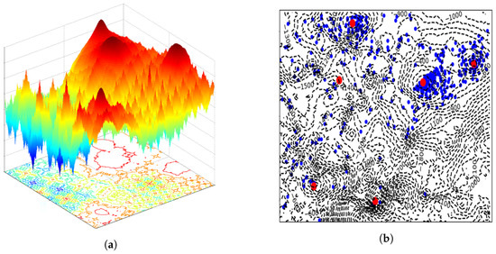
Figure 1.
Multimodal functions and their two-dimensional topographic maps.
The contributions of this study are as follows:
- Proposing an effective TCDE algorithm, which can effectively solve multimodal optimization problems in complex scenarios where multi-peaks are steeply connected and rough peaks coexist with fine peaks;
- Constructing complete topographical contours via geographical methods to guide the optimization of multimodal problems;
- Utilizing all historical individuals in the evolutionary process to construct the topographical profile, ensuring the rational utilization of every piece of historical information generated by the evolutionary algorithm;
- Dividing the peaks into coarse and fine peaks based on their characteristics and designing corresponding optimization strategies.
2. Related Work
2.1. General Approach to Solving Multimodal Optimization
The methods generally used to handle multimodal optimization problems include a series of evolutionary algorithms, such as DE, PSO, and the covariance matrix evolutionary algorithm.
Regarding DE algorithms for the solution of multimodal optimization problems, Dominico and Parpinelli [11] combined DBSCAN and two local search mechanisms with jDE and proposed NCjDE-2LSar, an adaptive differential evolution method based on the DBSCAN algorithm. Chen et al. [12] proposed the distributed individual differentiation evolution (DIDE) algorithm by allowing each individual to track a peak as a distributed unit, while introducing a lifetime mechanism and elite learning mechanism (ELM) in collaboration with the DIMP framework. Wang et al. [13] designed an adaptive DE (ADE) method with an adaptive parameter scheme based on two aspects of individual information for a novel local search technique, called fitness- and distance-based local search. This fitness information helps to avoid unhelpful local searching in local optimal points and similar regions, respectively.
Regarding PSO algorithms for the solution of multimodal optimization problems, Zhang et al. [14] introduced a neighborhood-based dynamic learning strategy, and Yang et al. [15] presented a stochastic, cognitively demonstrated particle swarm optimization algorithm (SCDLPSO). Two individual cognitive best positions are randomly selected from the entire population. The particle is then updated only if its own best position is outperformed by at least one of the selected positions. Qu et al. [16] proposed a grid-guided particle swarm optimizer, which uses the grid concept in the decision space to detect promising subregions and then generates multiple subpopulations accordingly.
The covariance matrix adaptive evolutionary strategies algorithm (CMAES) [17] puts the covariance information into a matrix, generates random points based on the information from this matrix, and tunes the parameters via a history step. Based on the combination of the strategies of exclusion of subpopulations and CMAES, Ahrari et al. [18] designed RS-CMA-ES, in which multiple subpopulations are explored in parallel. The offspring of the subpopulations is forced to keep a sufficient distance from the explored regions and the previously determined optimal solutions. Then, Ahrari et al. [19] put forward the RS-CMSA-ESII algorithm, which addresses the problems of the RS-CMSA-ES algorithm by proposing an adaptive scheme for the covariance matrices of the subpopulations, a stop criterion for the subpopulations, etc., thus improving the time complexity.
Experimental analyses of these methods show that they perform well in identifying multimodal scenarios where the transitions between peaks are gentle. They also demonstrate good recognition effects when the connections between peaks are steep but the peaks are uniformly distributed and similar in size. However, in complex situations—such as when peaks are steeply connected, their distribution exhibits low regularity, and there are both coarse and fine peaks—their performance is significantly worse. This indicates that multimodal optimization problems in complex scenarios still require extensive research.
2.2. Niching and Multimodal Optimization
Niching techniques are often combined with evolutionary algorithms [20] to solve multimodal optimization algorithms. The niching phenomenon refers to the preference of organisms with similar traits and characteristics to gather together in a specific environment [21]. Algorithms based on the niching concept can maintain a good global optimization ability while having a good rate of convergence, so they are particularly suitable for the optimization of complex multimodal functions.
Among niching technologies, the most commonly used strategies are crowding [22], speciation [23], clustering [24], fitness sharing [25], etc. Lin et al. [26] proposed a novel algorithm focusing on the formulation, balancing, and critical points of MMOPs, which uses nearest-better clustering (NBC) [27] to divide populations into multiple species and adaptively adjusts the size of each species.
Yue et al. [28] offered a new method to calculate crowding distances, which take the place of a weighted sum of Euclidean distances to neighbors. Zhao et al. [29] presented an adaptive DE (LBPADE) algorithm based on LBP [30], which locates multiple peaks by generating a niche via LBP, a mutation strategy with global interaction, and an adaptive parameter strategy to fully search for differentiated regions and maintain multiple peak regions. Gong et al. [31] developed NChOA, which embeds the niching technique in ChOA to solve MMOPs. Jiang et al. [32] considered the niche centroid determination problem as an optimization problem and proposed an NCD-DE method. Wang et al. [33] proposed SR-PSO-MAES, which is an adaptive particle swarm optimization method based on species division, species regulation, and local search that addresses the issue of a few species occupying the majority of the population in the iteration process.
Xiong et al. [34] proposed the enhanced adaptive neighborhood-based differential evolution (EANSDE) algorithm to efficiently address multimodal optimization problems (MMOPs). EANSDE retains poor solutions discarded in each generation and reintegrates them into the population once a predefined threshold is met. Additionally, it incorporates a mechanism to alleviate population congestion by eliminating highly similar individuals.
It can be seen from the above methods that a peak can be regarded as a niche, so niching is a very effective method in solving multimodal optimization. Determining niches, optimizing this search, and reducing the search workload in the niche are the main research focuses in this field at present.
2.3. Contours and Multimodal Optimization
Contours have been introduced into the multimodal optimization problem to guide optimization as they can carry more information than gradient descent. Wang et al. [10] proposed adaptive niche differential evolution (ANDE) to address multimodal optimization problems by combining affinity propagation clustering (PCA) and the contour prediction approach (CPA). They used the individual distribution information in each ecological niche to predict the rough locations of potential peaks and then further improved the accuracy of the algorithm through the two-level local search (TLLS).
The Kriging interpolation method can be used to construct contours and approximate the objective function, effectively transforming it into a continuous form to enhance the optimization performance. In scenarios involving highly complex functions, optimization algorithms can leverage Kriging interpolation [35] to estimate the objective function across the entire search space. In this way, the optimization approach can achieve the global or local optimal approximate solution. Zhan et al. [36] used an incremental Kriging model to transform a high-dimensional complex problem into a relatively simple agent model, which was then solved by an evolutionary algorithm. Song et al. [37] proposed a Kriging-assisted double-architecture evolutionary algorithm for each objective function to improve problem-solving. In the multimodal optimization algorithm, Wu et al. [38] obtained a Kriging model using all solutions in the population based on the Kriging operator and used it as a simplified model for the original problem. Currently, the Kriging method is rarely used in multimodal optimization problems, with existing methods primarily focused on transforming the objective functions of complex optimization problems into relatively simple proxy functions.
Despite the advanced nature of these modern multimodal optimization algorithms, they all have some limitations. The ordinary evolutionary algorithm excels in solving single peak problems; however, when facing multimodal problems, it often falls into local peaks and struggles to find all peaks. There are also some shortcomings in combining the niching technique with the evolutionary algorithm to solve the multimodal problem, such as setting the niche parameters, which can significantly affect the efficiency of the algorithm. Moreover, as mentioned in this paper, many of the evolutionary algorithms adopt greedy strategies, which lead to poor individuals being abandoned and not effectively used in the process of evolution. These heuristic strategies result in the loss of potential information. Finally, many methods rely solely on local information to guide the algorithm and do not use global information, which may lead to errors in the direction of the algorithm’s search.
3. Our Proposed TCDE Scheme
In the following, the TCDE algorithm that can be applied to the next generation of wireless communication networks is described. This section is divided into four main parts—namely, the application of DE for topographical exploration, the construction of topographical contours, the utilization of niching to explore landforms, and TCDE’s implementation.
3.1. Application of DE for Topographical Exploration
At the beginning of the TCDE algorithm, it is necessary to explore the terrain of the entire search space in order to guide the direction of algorithm evolution and generate suitable terrain contours. In Figure 2, the black dots represent the individuals used by the TCDE algorithm to generate the topographical contours. Obviously, the more accurately the terrain contour is obtained, the faster all peaks can be located.
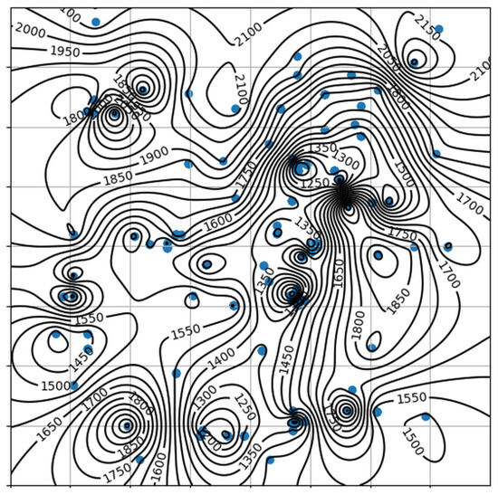
Figure 2.
Topographical contours generated from multimodal optimization problems.
As an efficient heuristic global optimization algorithm with good global exploration and convergence capabilities, the DE algorithm is widely employed in optimization algorithms, and it is therefore used in this study as the base algorithm.
3.1.1. Initialization
At the beginning of the TCDE algorithm, the initialization population is generated in the global search space. The population initialization is as shown in Equation (1):
where i represents the ith individual, j is the jth dimension, 0 is the 0th generation, and are the lower and upper limits of the jth-dimension coordinates for the multimodal optimization problem to be solved, and is a random number in the range .
The individuals generated by TCDE must be sufficiently diverse to enhance the global exploration capability. Hence, the global search space is divided into n subspaces of equal size based on the number of populations, and we generate individuals in each subspace according to Equation (1). At this time, and in Equation (1) are changed to the lower and upper limits of the jth-dimension coordinate of the subspace.
3.1.2. Mutation
In TCDE, two different mutation strategies are used—the DE/rand/1 strategy and the DE/current-to-pbest/1 strategy—which allows the algorithm to maintain good exploration capabilities while having a considerable convergence ability.
The DE/rand/1 strategy is as follows:
where , , and are randomly selected from the same generation, and g is denoted as the id of current generation. F is the variation factor, which is generally controlled within .
The DE/current-to-pbest/1 strategy is as follows:
where refers to the individual with the best fitness in the g-generation. The mutation vector may exceed the boundary limits, necessitating a boundary reset.
and are the lower and upper limits of the jth-dimension coordinate in the global range.
3.1.3. Crossover
After the mutation, a crossover between and is performed to generate the vector
where is the crossover rate, which generally takes values within . It determines the proportion of vector components inherited from the variant vectors. is a random integer chosen from 1 to N.
3.1.4. Selection
TCDE compares the newly generated individuals with and then selects individuals with good fitness to enter the next generation.
where is the fitness evaluation function.
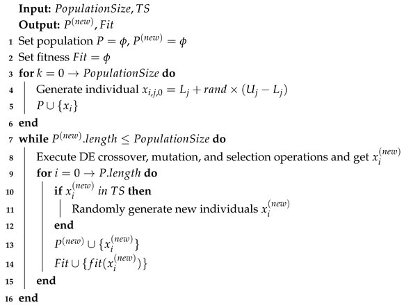
The regions where optimal values have already been identified are designated as taboo sections (TSs) in order to improve the ability of the next-generation population to explore new areas. As shown in Equation (7), if the currently selected offspring individual is located in a TS, the individual is discarded, and the selection is repeated. This process is described in Algorithm 1.
| Algorithm 1: Application of DE for topographical exploration |
 |
3.2. Constructing a Topographical Profile to Obtain an Initial Multimodal Distribution
In multimodal optimization problems, the visualized multimodal optimization function is very similar to topographic maps in geography. Multimodal optimization can be guided by the use of topographic maps as peaks and valleys can easily be identified.
3.2.1. Constructing Contours of Topographical Profiles
All individuals are used to construct the topographic contours. However, their distribution is often uneven, with some areas exhibiting significant gaps that require additional detail before contour plotting. In practice, to accurately represent the topographic surface, the space is uniformly divided into a set of raster grids. Missing data at unsampled raster points can be supplemented using Kriging interpolation.
The Kriging interpolation method estimates the value of unknown points via the weighted summation of the known points. It mainly employs the positional relationship and degree of correlation between the sampling points and the estimated points. This is an unbiased and linear optimal statistical method. Let be a sampling point in the region and be the observed value of the corresponding sampling point. The estimated value of the regionalized variable at x is denoted as follows:
where are the weight coefficients, and the values of each weight coefficient need to satisfy two conditions: unbiasedness and optimality.
A block processing strategy is adopted in this study to balance the fineness of the topographic map and computational efficiency. The entire 2D search space is uniformly divided into 4 quadrants (i.e., 4 parts), and, inside each quadrant, a resolution of 100 × 100 is used to define grid points. Thus, the total number of interpolated points for the entire topographic map is 4 parts × (100 × 100 points/part) = 40,000 grid points. This approach ensures sufficient detail while effectively managing the computational load.
3.2.2. Obtaining the Initial Potential Peaks
The TCDE algorithm searches for all potential peaks based on the obtained topographical profile.
In Figure 3, there is a neighborhood of individual i (surrounded by a solid circle) and a neighborhood of individual j (surrounded by a dashed circle). Then, Equation (9) is employed to determine potential peaks.
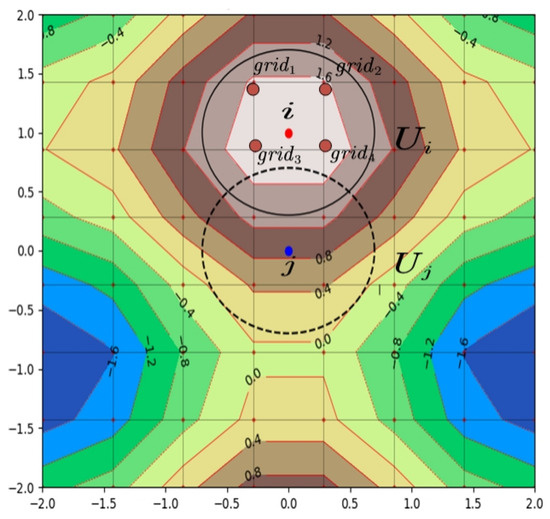
Figure 3.
Peak and topographical profile with grid points.
Here, is the potential peak found. is all the grid points within the neighborhood of the individual i. When the fitness of a real individual i is greater than the maximum fitness of the grid points within its neighborhood, i is regarded as a potential peak. The formula for the neighborhood setting of is shown in Equation (10). In general, the four nearest grid points to i are considered, but, in special cases when i is in the grid, the neighborhood range is moderately expanded.
is the set of potential peaks, as shown in Figure 4 and Algorithm 2.
| Algorithm 2: Constructing a topographical profile to get an initial multimodal distribution |
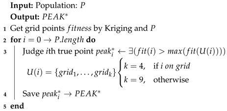 |
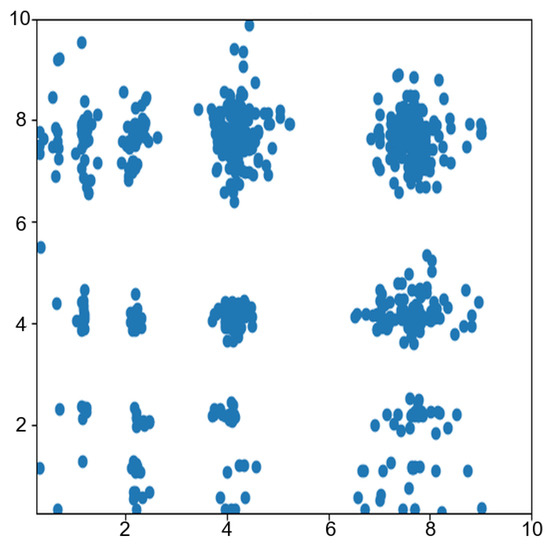
Figure 4.
Potential peaks.
3.3. Exploring Topographic Profiles by Using Niching
The potential peak set is obtained via TCDE, as described in the previous section. However, among these potential peaks, some potential peaks may belong to the same peak. As shown in Figure 5, , , and belong to the same peak. A detailed search in this region is thus needed to obtain the real peaks.
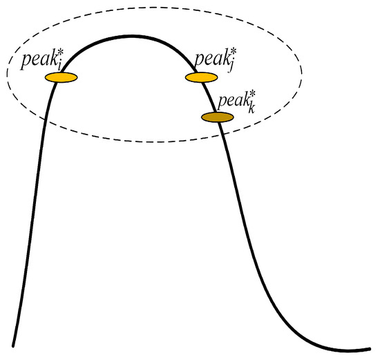
Figure 5.
Peak and peak range.
3.3.1. Building Niches
It is initially necessary to preprocess the potential peak set by selecting the top individuals in the neighborhood of . This reduces the algorithm’s computation time, as well as eliminating some of the possible noise. Then, these individuals are clustered by using DBSCAN to obtain multiple clusters. As shown in Figure 6, each cluster represents a niche. Assuming the existence of a peak in each niche, which is the best adapted individual i among the niches, the range of the niche is determined with i as the center of the circle. The radius of the niche is specified in Equation (12).
where denotes the location of the best-adapted individual in the niche. denotes the location of the worst-adapted individual.
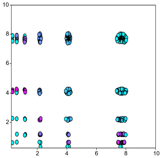
Figure 6.
After DBSCAN clustering.
3.3.2. Classifying Coarse and Fine Peaks
As shown in Figure 7, in complex multimodal optimization problems, there may be peaks with different range sizes. The peaks can be categorized into coarse and fine peaks according to their size. In general, peaks with a larger range (coarse peaks) are easily located, while smaller peaks (fine peaks) are difficult to find when their diameter is smaller than the current search step size.
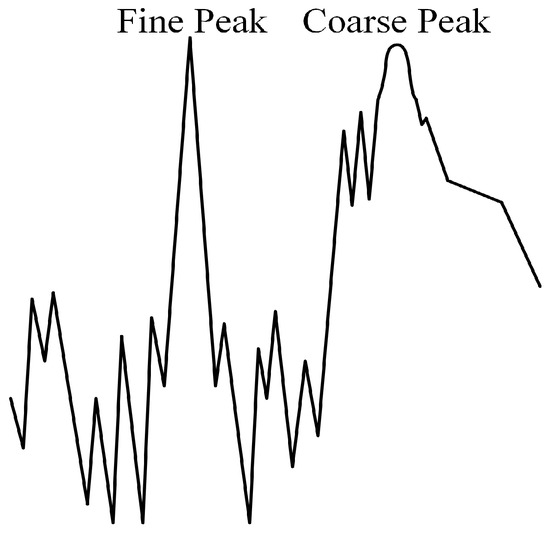
Figure 7.
Difference between coarse and fine peaks.
To address this situation, different strategies for optimization are adopted for TCDE. The judgment of the categories of peaks in TCDE is shown in Equation (13).
Here, refers to the type of the current peak. , which facilitates judgment.
3.3.3. Strategies for Coarse and Fine Peaks
Optimization strategies for both coarse and fine peaks are established on two levels: the taboo search (TS) radius is configured at the global level, while niche parameters are defined at the local level.
The TS is designed to prevent the algorithm from repeatedly exploring the already discovered peak areas. Once the niche search confirms and archives a new optimal peak, the system immediately creates a circular taboo region centered on the position of the peak. The radius of the TS is dynamically adjusted. Formula (14) is used to set a larger or smaller radius according to whether the peak is a “rough peak” or a “fine peak”.
where is the radius of the current TS and is the parameter controlling the radius.
In the subsequent DE exploration phase, any newly generated individual that falls within an existing TS is discarded and regenerated until it lands outside the taboo region. Here, the TS list is dynamically updated: whenever a new optimal peak is discovered, a new taboo region is added to the list.
In a niche, it is necessary to set two parameters: the learning step size and FEs. They are defined as follows:
The principle of setting the coarse peaks is to ensure a larger TS and learning step, and the FEs should be set to a smaller value. The setting principle for fine peaks is the opposite.
3.3.4. Searching for Peaks
In this step, a more detailed search of the obtained niches is conducted. In each niche, the TCDE algorithm runs DE to search for peaks. The DE/current-to-pbest/1 strategy, which is a greedy strategy that can greatly speed up convergence, is employed as the mutation strategy for DE.
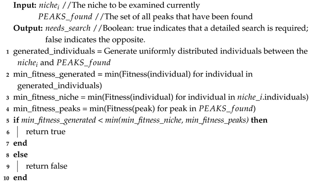
In order to avoid repeated searches, the TCDE algorithm uses the hill–valley strategy (Algorithm 3) on the niche before searching for peaks. Multiple individuals within the niche under investigation and all peaks already explored are uniformly generated. If the fitness of the generated individuals is lower than that of the aforementioned individuals, then it is determined that the current niche range has not reached the peak, and a detailed search is required. In the opposite case, no further search is required. The TS is updated according to the results at the end of the algorithm.
As shown in Algorithm 4, the input is , which is the potential peak set obtained by Algorithm 2. The TCDE algorithm screens and clusters this peak set to generate niches, where a new population is generated within each niche. A detailed search is conducted within the population to obtain the peak, and the taboo region TS is updated based on this information.
| Algorithm 3: Hill–valley check |
 |
| Algorithm 4: Application of niching for exploration of topographical appearance |
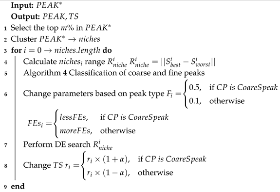 |
The TCDE method can be employed to obtain the final result by running the aforementioned Algorithms 1–4 in sequence until the FEs reach MaxFEs.
3.4. Time Complexity
The computational complexity of the TCDE algorithm is mainly represented by three core stages: (1) DE terrain exploration, (2) topographical contour construction, and (3) niche search.
First, DE terrain exploration is a standard differential evolution (DE) algorithm with computational complexity of . Here, D represents the number of data dimensions, and denotes the time cost for a single fitness function evaluation. Second, the computational complexity of constructing a topographical profile is demonstrated via Kriging interpolation, which is . Here, H is the total number of historical individuals used to build the contour, and is the number of grid points for interpolation. Finally, the niche search stage uses DBSCAN to cluster potential peak points for niche construction. The standard time complexity of DBSCAN is , where is the number of potential peak points used for clustering. After superimposing the local search, the complexity of this stage becomes , where is the number of niches generated after DBSCAN clustering, and is the cost of performing a local DE search in a single niche.
Therefore, the time complexity of TCDE is . Since H > N, the time complexity of TCDE is demonstrated by .
4. Performance Analysis
Eight benchmark functions (including both conventional and highly complex ones, as shown in Table 1) were selected from the CEC2013 competition dataset—which is commonly used for two-dimensional multimodal optimization research—in order to test the performance of the TCDE algorithm. For further comparison, 15 of the latest high-performance multimodal optimization algorithms were used as baseline methods. Finally, we explored how to apply TCDE to the next generation of wireless communication networks in engineering applications to address the multimodal optimization problems that exist within them.

Table 1.
Function introduction [39].
4.1. Evaluation Metrics
Given the maximum () and accuracy , the peak ratio () and success rate () were utilized to evaluate the performance of the multimodal optimization algorithms.
reflects the average percentage of all global optima found over multiple runs, with the following formula:
where denotes the global optimum found at the end of the ith run, represents the already known optimal value, denotes the number of runs, and stands for the number of successful runs.
is the percentage of successful runs (those in which all global optima are found). Its formula can be expressed as
Five precision classes are often used in the literature: = 1.0 × 10⁻¹, = 1.0 × 10⁻², = 1.0 × 10⁻³, = 1.0 × 10⁻⁴, and = 1.0 × 10⁻⁵. However, since the precision levels = 1.0 × 10⁻¹ and = 1.0 × 10⁻² are not sufficiently high, only the last three precision levels = 1.0 × 10⁻³, = 1.0 × 10⁻⁴, and = 1.0 × 10⁻⁵ were used here.
4.2. Baseline Methodology
The TCDE algorithm was compared with the following 15 multimodal optimization algorithms, mainly from highly cited works and authoritative journals (e.g., IEEE Transactions on Evolutionary Computation and IEEE Transactions on Cybernetics).
Firstly, since this method uses terrain contours to guide multimodal optimization, it is compared with other contour-based approaches.
- ANDE (2019) [10]: This method is characterized by utilizing the individual distribution information in each niche to generate contour lines, thereby predicting the approximate positions of potential peaks to accelerate the convergence speed.
Secondly, we selected multimodal optimization algorithms using subpopulation strategies as the baseline method to measure the performance of TCDE.
- CDE (2004) [22]: This method is characterized by fast convergence and the ability to finely tune the found results. It extends subpopulations via a crowding mechanism, enabling it to track and maintain multiple optimal solutions.
- SDE (2005) [23]: In each iteration, the algorithm adaptively forms multiple species (or subpopulations) within its DE population. Each species then operates as an independent DE algorithm, performing successive local improvements to eventually obtain multiple global optima.
- PNPCDE (2014) [40]: This method restricts member randomness without compromising exploration, using a parent-centric normalized neighborhood (PCNN) mutation operator combined with a synchronous crowding replacement strategy. This approach effectively prevents niche loss, reduces genetic drift, and maintains optimal solutions, enabling stable and efficient niching behavior.
- Self-CSDE (2014) [24]: This method divides the population into subpopulations using clustering and then uses adaptive parameter control to enhance the search capability of the species-based differential evolution (SDE) algorithm, and the method has achieved good results.
- NMMSO (2014) [41]: The subpopulations of the algorithm are each responsible for optimizing independent local modes. If individuals within a subpopulation are identified as being near other peaks, they are allowed to migrate from the original subpopulation; if different subpopulations are determined to target the same peak, they are merged. The algorithm achieves optimization by dynamically managing multiple particle swarms in this way.
- NCD-DE (2021) [32]: This method designs a fitness–entropy measurement objective function, applies an internal genetic algorithm (GA) to optimize multiple promising niche centers, and globally cooperates with subpopulation niching using these centers to generate new individuals. Differential evolution (DE) is then employed iteratively to refine the results.
- RS-CMSA-ESII (2022) [19]: This method proposes a covariance matrix adaptation evolution strategy with repulsive subpopulations. It optimizes the subpopulation initialization process and designs more precise key forbidden regions.
Finally, a group of multimodal optimization algorithms using local information was selected as the comparison methods.
- R3PSO (2010) [42]: The main feature of this method is the adoption of a simple and effective parameter-free niching algorithm—namely, using a ring neighborhood topology to induce the formation of stable niches. It preserves the current best position through the local memory of individual particles, while using the particle swarm optimization (PSO) algorithm as a local optimizer to obtain the final results.
- LIPS (2013) [43]: The Locally Informed Particle Swarm (LIPS) algorithm forms niches by calculating Euclidean distance neighborhoods, using local information to enhance the local search capabilities. It employs multiple local best particles to guide each particle’s search, thus identifying multiple optimal solutions via the fine-tuning ability of particle swarm optimization (PSO).
- LoISDE (2014) [44]: This method first employs a local information matrix to enhance the mutation phase of DE. Then, it integrates this refined mutation phase with an information-sharing mechanism to elevate the algorithm’s search efficiency. Subsequently, it implements a niche-aware population synchronization strategy to minimize niche loss. Together, these sequential strategies empower LoINDE to outperform existing DE-based niching algorithms.
- LMCEDA and LMSEDA (2017) [45]: A novel local search scheme based on Gaussian distribution was proposed to refine the obtained solutions, thereby constructing the Local Search Clustering-Enhanced Distribution Estimation Algorithm (LMCEDA) and the Local Search Speciation Distribution Estimation Algorithm (LMSEDA).
- FDLS-ADE (2023) [13]: This method proposes a novel fitness- and distance-based individual local search technique, FDLS, which can avoid ineffective local searching in local optimal solutions and similar regions. After applying FDLS to DE with an adaptive parameter scheme, the effectiveness of the algorithm has been significantly improved.
- SA-DQN-DE (2024) [9]: This method assigns mutation operations to each individual based on the effectiveness of different mutation operators in historical evolution. Then, deep reinforcement learning is introduced to select multiple local search operators to improve the accuracy of potential optimal solutions.
4.3. Parameter Settings
The population sizes and maximum numbers of fitness evaluations of the TCDE algorithm are shown in Table 2. The mutation rate F and crossover rate in TCDE were set to and , respectively. In the stage of seeking niches, the TCDE algorithm employs DBSCAN to cluster the top 10% of all potential peaks that have been discovered, and the neighborhood radius of individuals in DBSCAN was set to 0.08. All baseline methods employed the same population size N and as in Table 1. The experiments were performed on a PC with four Intel Core i5-8400 2.80 GHz CPUs, 16 GB of RAM, and the Windows 10 64-bit system. All algorithms were run independently multiple times for each function, and the average results are reported.
Table 2.
Population size and maximum number of fitness evaluations [39].
4.4. Analysis of Experimental Results
To facilitate an intuitive understanding of TCDE, Figure 8 presents the ultimate outcomes achieved with TCDE for eight distinct functions. From Figure 8, it becomes evident that the TCDE algorithm effectively identifies all peak points within these eight functions. These functions encompass not only simpler ones, such as F4(a) and F5(b), but also more intricate functions like F6(c), F7(d), and F10(e), which possess numerous peak points. Furthermore, even in the case of highly complex functions such as F12(g) and F13(h), which contain many local optima, the TCDE algorithm consistently and accurately pinpoints all peaks with the guidance provided by the topographical contours.
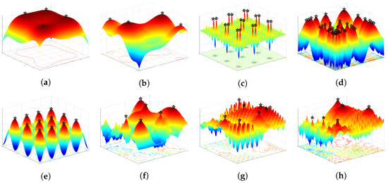
Figure 8.
Final population results for eight functions. (a) F4. (b) F5. (c) F6. (d) F7. (e) F10. (f) F11. (g) F12. (h) F13.
To further analyze the performance of the TCDE algorithm, it was compared with the baseline methods using different precision levels: = 1.0 × 10⁻³, = 1.0 × 10⁻⁴, and = 1.0 × 10⁻⁵. As shown in Table 3, Table 4 and Table 5, the TCDE algorithm outperformed the other algorithms in all eight test functions evaluated with the and .
Table 3.
Comparison of PR and SR for two-dimensional functions at accuracy level .
Table 4.
Comparison of PR and SR for two-dimensional functions at accuracy level .
Table 5.
Comparison of PR and SR for two-dimensional functions at accuracy level .
Both the TCDE and AnDE algorithms perform well, but the former outperforms the latter (which uses contour methods) on F7 and F13. As shown in Figure 8, these two test functions involve complex scenarios with coexisting rough and fine peaks, as well as steep connections between peaks. This indicates that, compared with the AnDE algorithm’s local application of contour optimization, the TCDE algorithm’s strategy of globally optimizing topographical contours while distinguishing between rough and fine peaks is effective, enabling it to handle multimodal optimization problems in complex situations.
As shown in Table 3, Table 4 and Table 5, all baseline methods in the subpopulation group perform worse than TCDE. Among them, Self-CSDE shows extremely poor performance: its PR and SR values are only 1.000 for the F5 function in Table 3, and it fails to achieve perfect results for any other test functions. This indicates that its niche strategy of adaptively generating subpopulations fails in complex scenarios with steep connections between multimodal peaks and coexisting rough–fine peaks. CDE, SDE, and PNPCDE can effectively handle scenarios with gentle or steep connections between multimodal peaks, but their strategies perform poorly in complex cases with rough–fine peaks. Although RS-CMSA-ESII demonstrates improved performance, it still has a probability of failure in dealing with steep connections between multimodal peaks and complex situations with coexisting rough–fine peaks.
Similarly, it is evident that TCDE outperforms the baseline methods relying on local information. Here, methods such as LIPS, R3PSO, and LolSDE, which primarily depend on local information strategies, struggle to locate all peaks in both scenarios with gentle connections between multimodal peaks and more complex ones. When local information is combined with strategies such as Gaussian distribution and fitness–distance enhancement, the multimodal optimization capabilities of the algorithms are enhanced. For instance, LMCEDA, LMSEDA, and FDLS-ADE can not only handle gentle connections between multimodal peaks but also demonstrate significantly improved performance in scenarios with steep connections. In particular, SA-DQN-DE, after integrating deep learning, exhibits enhanced capabilities in addressing complex scenarios with coexisting rough and fine peaks.
From the above analysis, it can be seen that the TCDE algorithm can be applied to simple and complex multimodal optimization problems, including those with gentle and steep connections between multiple peaks and coexisting rough–fine peaks. To further highlight this characteristic of the TCDE algorithm, F7 (2D Vincent) and F13 (2D Composition Function 3), as two test functions with complex characteristics, were selected for detailed analysis.
4.4.1. F7 (2D Vincent)
The F7 function is shown in Figure 9. It has 36 peaks with different sizes and contains multiple different coarse and fine peaks, with complex terrain and landforms. This function challenges the capabilities of the multimodal optimization algorithm.
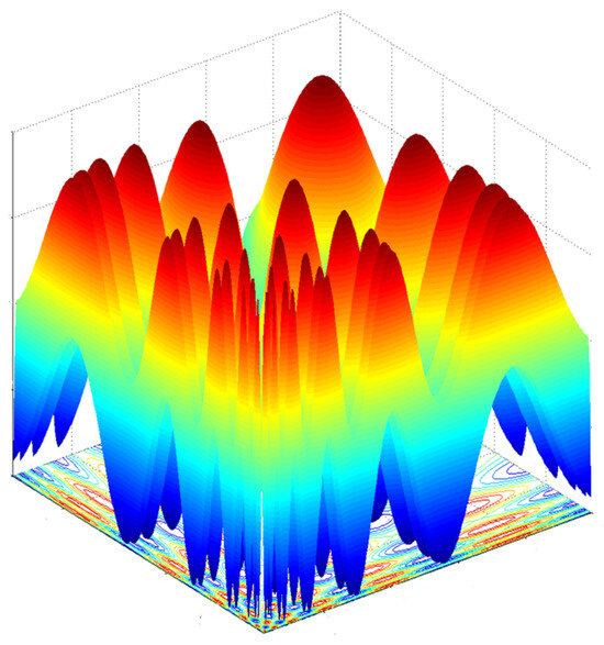
Figure 9.
Three-dimensional image of 2D Vincent function.
Figure 10 shows the range of potential peaks predicted by the TCDE algorithm in rounds 1, 10, 20, and 30 of the optimization of the 2D Vincent function by means of terrain contours. From Figure 10, it is evident that the TCDE algorithm identifies some of the peaks in the first round, and, as the algorithm iterates, more potential peaks are discovered. In other words, the number of individuals in the potential peak area also increases. This means that peaks are located more accurately.
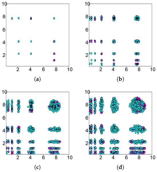
Figure 10.
Four stages of optimizing the 2D Vincent function. (a–d) show the optimization process at different iterations.
The distribution of individuals in the TCDE algorithm’s topographical exploration after setting taboo areas is shown in Figure 11. It can be seen that, as the algorithm iterates, the taboo regions also constantly change. This causes the population to constantly move away from the positions where the peaks have been explored during the evolution of the algorithm. In this way, the TCDE algorithm can explore areas that were previously underexplored more carefully.
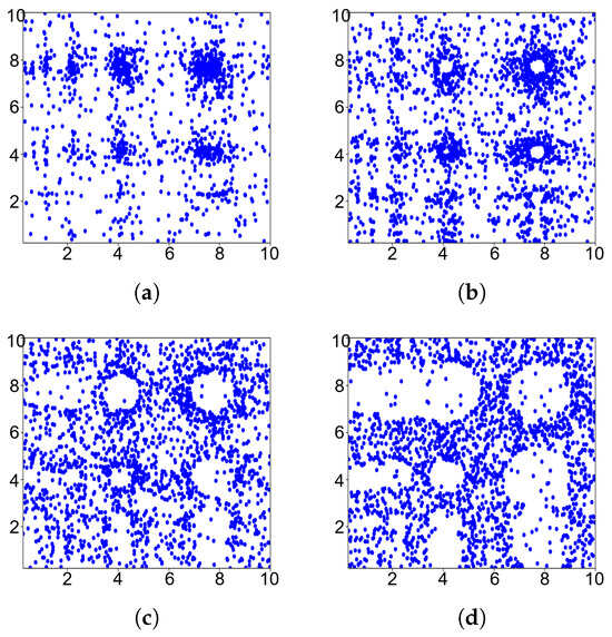
Figure 11.
Individual distribution of 2D Vincent function with TS for topographical exploration when applying DE (a–d).
Through the above two techniques, the TCDE algorithm can effectively address the problem of coarse and fine peaks in the 2D Vincent function. Thus, all peaks are identified.
4.4.2. F13 (2D Composition Function 3)
Figure 8h shows F13, which is a more complex multimodal optimization function than F7, consisting of six basic functions, including the Weierstrass function and Griewank’s function. The peaks in 2D Composition Function 3 include both coarse and fine peaks. The fine peaks display a remarkable level of irregularity, justifying this function’s classification as a classic complex multimodal problem. Similar to the procedure used for the 2D Vincent function, the ranges of potential peaks accurately predicted in rounds 1, 10, 20, and 30 were selected. As shown in Figure 12, the TCDE algorithm finds all coarse peaks, as well as some of the fine peaks at the beginning. As the algorithm iterates, the taboo areas of the coarse peaks gradually expand, forcing the population to stay away from the peaks that have been found. This is shown in Figure 13. Finally, as the TCDE algorithm iterates, the topographic contours of 2D Composition Function 3 become increasingly obvious. Very small peaks that were previously difficult to explore are also successfully discovered, which clearly illustrates the superiority of the TCDE algorithm.
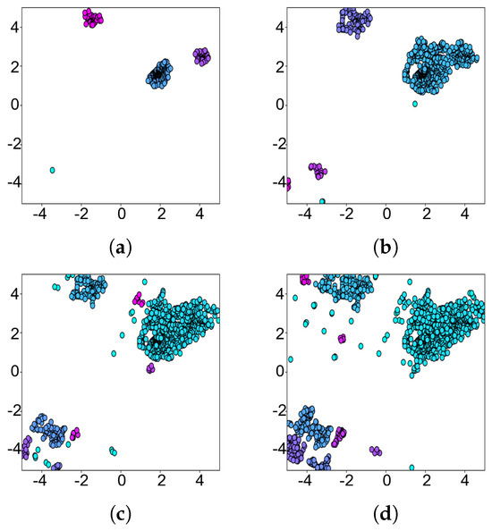
Figure 12.
Four stages of optimizing Composition Function 3 (a–d).
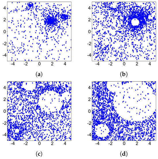
Figure 13.
Individual distribution of Composition Function 3 with TS for topographical exploration when applying DE (a–d).
4.5. Engineering Applications
There are numerous multimodal optimization problems in engineering applications, such as the multi-template matching problem in image recognition. These problems have wide-ranging applications in fields such as medicine, transportation, and industrial automation and thus hold considerable research value. For instance, in the realm of electronics manufacturing, the PCB multi-template matching problem involves employing template matching technology to precisely locate various components on the PCB, including resistors, capacitors, and integrated circuits, ensuring that they are correctly placed. Moreover, PCB multi-template matching can be utilized to detect defects on the PCB, such as soldering issues, open circuits, or short circuits, facilitating early identification and repair and thereby ensuring product quality. While traditional template matching can only be used to identify a single matching position, in practical engineering applications, there are typically multiple matching positions. Additionally, traditional template matching algorithms often necessitate the traversal of every pixel, which can lead to substantial costs and time consumption. Therefore, the ability to identify multiple peaks simultaneously using fewer pixels could significantly reduce the costs and enhance the efficiency of businesses.
Evolutionary algorithms can effectively address this issue of traditional template matching. Evolutionary algorithms seek the optimal solution through randomized populations, employing operations such as crossover and mutation, thus circumventing the need to inspect every pixel. This approach offers a significant advantage in terms of efficiency. When multiple regions within the target image match the template, the relationship between the template’s pixel positions and the matching degree forms a multimodal optimization problem. Consequently, the TCDE algorithm can be employed to effectively solve this problem.
A similarity evaluation function must be employed to transform PCB multi-template matching into a multi-peak optimization problem. Normalized cross-correlation (NCC) is a technique that involves quantifying the similarity between each pixel of a target image and a template. The NCC matching method involves calculating the cross-correlation between the target image and the template, normalizing the result, and then assessing the similarity between each pixel in the target image and the template. This process mitigates the effects of varying brightness and contrast levels, enhancing the accuracy of the similarity measurement. Consequently, NCC has long been recognized as a standard method for similarity measurement in feature matching and target recognition. This indicates that the TCDE algorithm is effective in the PCB multi-template matching problem.
Template matching can be transformed into a multimodal optimization problem through the use of normalized cross-correlation (NCC) matching. The normalized cross-correlation matching between a target image F of size and a template T of size at position is defined by Equation (19), where and represent the grayscale values at position in the target image and the template image, respectively. F and T denote the average grayscale values of overlapping regions between the target image and the template image and the grayscale average value of the template image, respectively. The template moves within the range of the target image, and the matching degree between corresponding pixels of T and F is calculated using the NCC method. is a normalized value within the range . A higher matching degree between T and F corresponds to a larger value of . The matching degree of the template image at various positions within the target image can be determined by comparing the similarity between two images and identifying their correlation. Subsequently, the TCDE algorithm can be employed to search for multiple peaks, thereby identifying multiple optimal solutions.
Figure 14 depicts the target PCB image with dimensions of 393 pixels × 422 pixels, while Figure 15 illustrates a template resistor image that is 34 pixels × 51 pixels in size. Within the target PCB image, there are four regions that resemble the pattern in the template resistor image, indicating the presence of four peaks. The matching process transforms into a multi-peak optimization function after the application of NCC, as depicted in Figure 16. From the graph, it can be observed that this is a standard multi-peak optimization problem, with four peaks in the search space, representing the four optimal matching positions. Additionally, there are many irregular local peaks in the search space, which are significant sources of interference. The objective is to avoid all local peaks while accurately identifying all global ones. However, due to the abundance of local peaks, the algorithm can easily become trapped, making it difficult to locate the global peaks, which are narrow and hard to detect. As a result, the problem poses significant challenges.
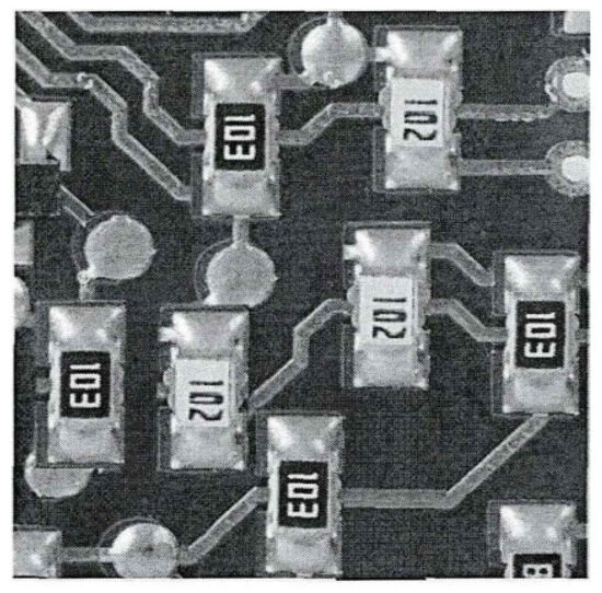
Figure 14.
Target PCB image.
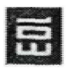
Figure 15.
Template image.
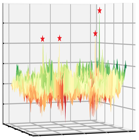
Figure 16.
Three-dimensional PCB target image and template image matching diagram.
Table 6 below summarizes the performance of the improved TCDE algorithm for different population sizes (30, 50, 100, 150) and compares it with the experimental results of various multi-peak optimization algorithms. Unlike the previously used evaluation metrics, which were suitable for continuous solution spaces of multi-peak optimization functions, the current image multi-target recognition involves a finite search space. Specifically, the pixel size of target image 3 is 393 × 422 = 165,846. Therefore, the original metrics are no longer applicable to the current algorithm. The number of detected pixels, which represents the consumed FEs during the optimization process, was used as a performance metric in this experiment to demonstrate the effectiveness of the algorithm. The use of fewer pixels used when finding all peaks indicates better algorithm performance.
Table 6.
Comparison results of multimodal optimization algorithms using NCC.
Table 6 displays the comparison results of the TCDE algorithm with 15 advanced multi-peak optimization algorithms for different population sizes for the PCB multi-template recognition problem, with the similarity evaluation function being NCC. The experimental results indicate that the TCDE algorithm consistently uses the fewest pixels. This demonstrates the superiority of the TCDE algorithm and its effectiveness in solving image multi-target recognition problems.
5. Conclusions and Future Work
In this study, geography-like landforms were derived from fitness contour lines within the context of multimodal optimization problems, and subsequent optimization was guided by the extracted geomorphic information. This method utilizes all individuals to construct a topographical contour, enhanced by Kriging interpolation to capture finer details, resulting in a comprehensive representation of the global landscape. Potential peaks are identified based on these detailed global geomorphic data. Niches are then formed through clustering techniques, and the optimal solutions are found by conducting an exhaustive search within each niche. Experiments show that the TCDE algorithm can locate all peak regions in all eight test functions. In other words, compared with the baseline method, the strategy adopted in this method is very effective, and it can adapt well to complex situations where multi-peaks are gently or steeply connected and rough peaks coexist with fine peaks. Through engineering application analysis, it was found that the TCDE algorithm can be effectively applied to multimodal optimization problems such as template matching. However, the TCDE algorithm has high time complexity of . In high-dimensional cases, Kriging interpolation needs to be performed pairwise between dimensions, which greatly increases the time complexity. Therefore, future work will focus on studying suitable interpolation methods with low time complexity for multimodal optimization problems, such that the TCDE method can be applied to high-dimensional multimodal optimization problems.
Author Contributions
Methodology, Z.C. and L.J.; writing—original draft, Z.C., Y.Z., C.F., X.G. and H.J.; writing—review and editing, L.J. and Z.C. All authors have read and agreed to the published version of the manuscript.
Funding
This research was funded by the Open Fund Project of the Key Laboratory of Smart Earth (Grant No. KF2023YB04-04).
Data Availability Statement
The code can be downloaded at https://github.com/2573723684/TCDE (accessed on 21 May 2025).
Conflicts of Interest
The authors declare no conflicts of interest.
References
- Daramola, G.O.; Jacks, B.S.; Ajala, O.A.; Akinoso, A.E. AI applications in reservoir management: Optimizing production and recovery in oil and gas fields. Comput. Sci. Res. J. 2024, 5, 972–984. [Google Scholar]
- Gherold, V.; Mandralis, I.; Sihite, E.; Salagame, A.; Ramezani, A.; Gharib, M. Self-supervised cost of transport estimation for multimodal path planning. IEEE Robot. Autom. Lett. 2025, 10, 6872–6879. [Google Scholar] [CrossRef]
- Alhijawi, B.; Awajan, A. Genetic algorithms: Theory, genetic operators, solutions, and applications. Evol. Intell. 2024, 17, 1245–1256. [Google Scholar] [CrossRef]
- Daviran, M.; Maghsoudi, A.; Ghezelbash, R. Optimized ai-mpm: Application of pso for tuning the hyperparameters of svm and rf algorithms. Comput. Geosci. 2025, 195, 105785. [Google Scholar] [CrossRef]
- Pesaramelli, R.S.; Sujatha, B. Principle correlated feature extraction using differential evolution for improved classification. AIP Conf. Proc. 2024, 2919, 070001. [Google Scholar]
- Liang, S.M.; Wang, Z.J.; Huang, Y.B.; Zhan, Z.H.; Kwong, S.; Zhang, J. Niche center identification differential evolution for multimodal optimization problems. Inf. Sci. 2024, 678, 121009. [Google Scholar] [CrossRef]
- Awadallah, M.A.; Makhadmeh, S.N.; Al-Betar, M.A.; Dalbah, L.M.; Al-Redhaei, A.; Kouka, S.; Enshassi, O.S. Multi-objective ant colony optimization. Arch. Comput. Methods Eng. 2025, 32, 995–1037. [Google Scholar] [CrossRef]
- Romasevych, Y.; Loveikin, V.; Brand, Z. Influence of swarm connectivity on l-best pso performance. In Proceedings of the 2024 IEEE 5th KhPI Week on Advanced Technology (KhPIWeek), Kharkiv, Ukraine, 7–11 October 2024; pp. 1–5. [Google Scholar]
- Liao, Z.; Pang, Q.; Gu, Q. Differential evolution based on strategy adaptation and deep reinforcement learning for multimodal optimization problems. Swarm Evol. Comput. 2024, 87, 101568. [Google Scholar] [CrossRef]
- Wang, Z.-J.; Zhan, Z.-H.; Lin, Y.; Yu, W.-J.; Wang, H.; Kwong, S.; Zhang, J. Automatic niching differential evolution with contour prediction approach for multimodal optimization problems. IEEE Trans. Evol. Comput. 2019, 24, 114–128. [Google Scholar] [CrossRef]
- Dominico, G.; Parpinelli, R.S. Multiple global optima location using differential evolution, clustering, and local search. Appl. Soft Comput. 2021, 108, 107448. [Google Scholar] [CrossRef]
- Chen, Z.-G.; Zhan, Z.-H.; Wang, H.; Zhang, J. Distributed individuals for multiple peaks: A novel differential evolution for multimodal optimization problems. IEEE Trans. Evol. Comput. 2019, 24, 708–719. [Google Scholar] [CrossRef]
- Wang, Z.-J.; Zhan, Z.-H.; Li, Y.; Kwong, S.; Jeon, S.-W.; Zhang, J. Fitness and distance based local search with adaptive differential evolution for multimodal optimization problems. IEEE Trans. Emerg. Top. Comput. Intell. 2023, 7, 684–699. [Google Scholar] [CrossRef]
- Zhang, X.; Liu, H.; Tu, L. A modified particle swarm optimization for multimodal multi-objective optimization. Eng. Appl. Artif. Intell. 2020, 95, 103905. [Google Scholar] [CrossRef]
- Yang, Q.; Hua, L.; Gao, X.; Xu, D.; Lu, Z.; Jeon, S.-W.; Zhang, J. Stochastic cognitive dominance leading particle swarm optimization for multimodal problems. Mathematics 2022, 10, 761. [Google Scholar] [CrossRef]
- Qu, B.; Li, G.; Yan, L.; Liang, J.; Yue, C.; Yu, K.; Crisalle, O.D. A grid-guided particle swarm optimizer for multimodal multi-objective problems. Appl. Soft Comput. 2022, 117, 108381. [Google Scholar] [CrossRef]
- Song, S.; Zhang, B.; Chen, X.; Xu, Q.; Qu, J. Wart-treatment efficacy prediction using a cma-es-based dendritic neuron model. Appl. Sci. 2023, 13, 6542. [Google Scholar] [CrossRef]
- Ahrari, A.; Deb, K.; Preuss, M. Multimodal optimization by covariance matrix self-adaptation evolution strategy with repelling subpopulations. Evol. Comput. 2017, 25, 439–471. [Google Scholar] [CrossRef]
- Ahrari, A.; Elsayed, S.; Sarker, R.; Essam, D.; Coello, C.A. Static and dynamic multimodal optimization by improved covariance matrix self-adaptation evolution strategy with repelling subpopulations. IEEE Trans. Evol. Comput. 2022, 26, 527–541. [Google Scholar] [CrossRef]
- Liang, R.; Xing, Y.; Hu, L. Enhancing energy efficiency by improving internet of things devices security in intelligent buildings via niche genetic algorithm-based control technology. Appl. Sci. 2023, 13, 10717. [Google Scholar] [CrossRef]
- Mahfoud, S.W. Niching Methods for Genetic Algorithms; University of Illinois at Urbana-Champaign: Champaign, IL, USA, 1995. [Google Scholar]
- Thomsen, R. Multimodal optimization using crowding-based differential evolution. In Proceedings of the 2004 Congress on Evolutionary Computation (IEEE Cat. No. 04TH8753), Portland, OR, USA, 19–23 June 2004; Volume 2, pp. 1382–1389. [Google Scholar]
- Li, X. Efficient differential evolution using speciation for multimodal function optimization. In Proceedings of the 7th Annual Conference on Genetic and Evolutionary Computation, Washington, DC, USA, 25–29 June 2005; pp. 873–880. [Google Scholar]
- Gao, W.; Yen, G.G.; Liu, S. A cluster-based differential evolution with self-adaptive strategy for multimodal optimization. IEEE Trans. Cybern. 2013, 44, 1314–1327. [Google Scholar] [CrossRef]
- Ursem, R.K. Multinational evolutionary algorithms. In Proceedings of the 1999 Congress on Evolutionary Computation-CEC99 (Cat. No. 99TH8406), Washington, DC, USA, 6–9 July 1999; Volume 3, pp. 1633–1640. [Google Scholar]
- Lin, X.; Luo, W.; Xu, P. Differential evolution for multimodal optimization with species by nearest-better clustering. IEEE Trans. Cybern. 2019, 51, 970–983. [Google Scholar] [CrossRef] [PubMed]
- Fowlkes, C.; Belongie, S.; Chung, F.; Malik, J. Spectral grouping using the nystrom method. IEEE Trans. Pattern Anal. Mach. Intell. 2004, 26, 214–225. [Google Scholar] [CrossRef] [PubMed]
- Yue, C.; Suganthan, P.N.; Liang, J.; Qu, B.; Yu, K.; Zhu, Y.; Yan, L. Differential evolution using improved crowding distance for multimodal multiobjective optimization. Swarm Evol. Comput. 2021, 62, 100849. [Google Scholar] [CrossRef]
- Zhao, H.; Zhan, Z.-H.; Lin, Y.; Chen, X.; Luo, X.-N.; Zhang, J.; Kwong, S.; Zhang, J. Local binary pattern-based adaptive differential evolution for multimodal optimization problems. IEEE Trans. Cybern. 2019, 50, 3343–3357. [Google Scholar] [CrossRef]
- Ojala, T.; Pietikainen, M.; Maenpaa, T. Multiresolution gray-scale and rotation invariant texture classification with local binary patterns. IEEE Trans. Pattern Anal. Mach. Intell. 2002, 24, 971–987. [Google Scholar] [CrossRef]
- Gong, S.-P. Mohammad Khishe, and Mokhtar Mohammadi. Niching chimp optimization for constraint multimodal engineering optimization problems. Expert Syst. Appl. 2022, 198, 116887. [Google Scholar] [CrossRef]
- Jiang, Y.; Zhan, Z.-H.; Tan, K.C.; Zhang, J. Optimizing niche center for multimodal optimization problems. IEEE Trans. Cybern. 2021, 53, 2544–2557. [Google Scholar] [CrossRef]
- Wang, R.; Hao, K.; Huang, B.; Zhu, X. Adaptive niching particle swarm optimization with local search for multimodal optimization. Appl. Soft Comput. 2023, 133, 109923. [Google Scholar] [CrossRef]
- Xiong, S.; Gong, W.; Wang, K. An adaptive neighborhood-based speciation differential evolution for multimodal optimization. Expert Syst. Appl. 2023, 211, 118571. [Google Scholar] [CrossRef]
- Cressie, N. The origins of kriging. Math. Geol. 1990, 22, 239–252. [Google Scholar] [CrossRef]
- Zhan, D.; Xing, H. A fast kriging-assisted evolutionary algorithm based on incremental learning. IEEE Trans. Evol. Comput. 2021, 25, 941–955. [Google Scholar] [CrossRef]
- Song, Z.; Wang, H.; He, C.; Jin, Y. A kriging-assisted two-archive evolutionary algorithm for expensive many-objective optimization. IEEE Trans. Evol. Comput. 2021, 25, 1013–1027. [Google Scholar] [CrossRef]
- Wu, X.; Lin, Q.; Lin, W.; Ye, Y.; Zhu, Q.; Leung, V.C.M. A kriging model-based evolutionary algorithm with support vector machine for dynamic multimodal optimization. Eng. Appl. Artif. Intell. 2023, 122, 106039. [Google Scholar] [CrossRef]
- Li, X.; Engelbrecht, A.; Epitropakis, M.G. Benchmark Functions for cec’2013 Special Session and Competition on Niching Methods for Multimodal Function Optimization; Technical Report; RMIT University, Evolutionary Computation and Machine Learning Group: Melbourne, Australia, 2013. [Google Scholar]
- Biswas, S.; Kundu, S.; Das, S. An improved parent-centric mutation with normalized neighborhoods for inducing niching behavior in differential evolution. IEEE Trans. Cybern. 2014, 44, 1726–1737. [Google Scholar] [CrossRef] [PubMed]
- Fieldsend, J.E. Running up those hills: Multi-modal search with the niching migratory multi-swarm optimiser. In Proceedings of the 2014 IEEE Congress on Evolutionary Computation (CEC), Beijing, China, 6–11 July 2014; pp. 2593–2600. [Google Scholar]
- Li, X. Niching without niching parameters: Particle swarm optimization using a ring topology. IEEE Trans. Evol. Comput. 2010, 14, 150–169. [Google Scholar] [CrossRef]
- Qu, B.-Y.; Suganthan, P.N.; Das, S. A distance-based locally informed particle swarm model for multimodal optimization. IEEE Trans. Evol. Comput. 2013, 17, 387–402. [Google Scholar] [CrossRef]
- Biswas, S.; Kundu, S.; Das, S. Inducing niching behavior in differential evolution through local information sharing. IEEE Trans. Evol. Comput. 2014, 19, 246–263. [Google Scholar] [CrossRef]
- Yang, Q.; Chen, W.-N.; Li, Y.; Chen, C.L.P.; Xu, X.-M.; Zhang, J. Multimodal estimation of distribution algorithms. IEEE Trans. Cybern. 2017, 47, 636–650. [Google Scholar] [CrossRef]
Disclaimer/Publisher’s Note: The statements, opinions and data contained in all publications are solely those of the individual author(s) and contributor(s) and not of MDPI and/or the editor(s). MDPI and/or the editor(s) disclaim responsibility for any injury to people or property resulting from any ideas, methods, instructions or products referred to in the content. |
© 2025 by the authors. Licensee MDPI, Basel, Switzerland. This article is an open access article distributed under the terms and conditions of the Creative Commons Attribution (CC BY) license (https://creativecommons.org/licenses/by/4.0/).