A Low-Cost Arduino-Based I–V Curve Tracer with Automated Load Switching for PV Panel Characterization

Abstract

Accurate photovoltaic (PV) panel characterization is critical for optimizing renewable energy systems, but it is often hindered by the high cost of commercial tracers or the slow, error-prone nature of manual methods. This paper presents a low-cost, Arduino-based I–V curve tracer that overcomes these limitations through fully automated resistive load switching. By integrating a relay-controlled resistor bank managed by a single microcontroller, the system eliminates the need for manual intervention, enabling rapid and repeatable measurements in just 45 s. This rapid acquisition is a key advantage over manual systems, as it minimizes the impact of fluctuating environmental conditions and ensures the resulting I–V curve represents a stable operating point. Compared to commercial alternatives, our open-source solution offers significant benefits in cost, portability, and flexibility, making it ideal for field deployment. The system’s use of fixed, stable resistive loads for each measurement point also ensures high repeatability and straightforward comparison with theoretical models. Experimental validation demonstrated high agreement with a single-diode PV model, achieving a mean absolute percentage error (MAPE) of 4.40% against the manufacturer’s data. Furthermore, re-optimizing the model with field-acquired data reduces the MAPE from 18.23% to 7.06% under variable irradiance. This work provides an accessible, robust, and efficient tool for PV characterization, democratizing access for research, education, and field diagnostics.

1. Introduction

Recent developments in sustainable energy supply can be directly related to the energy transition to renewable sources, since these are not only relatively clean sources, but can also be used in a decentralized manner [1]. In recent years, clean energy technologies have gained ground, causing a decrease in the demand for fossil fuels such as coal, natural gas, and oil. Projections suggest that this trend will continue, with fossil fuel demand declining by an average of 3 exajoules (EJ) per year until 2050. The peak demand is expected to occur around 2030 [2].

For a higher transition from fossil fuels to renewable sources, this process should be affordable. Addressing the initial expenses associated with clean energy technologies will be crucial in promoting their adoption, particularly among households with lower incomes [2].

To optimize the performance of renewable energy generators, such as photovoltaic panels, it is essential to gather detailed information on how they operate under various conditions. This allows real-time data collection over extended periods, with easy storage and accessibility [3,4].

While measuring voltage and current effectively provides information about the power of photovoltaic panels (PV), fully characterizing these devices requires varying the load they are subjected to. By doing so, the characteristic curves of the panel can be obtained. However, due to rapidly changing and unpredictable field conditions, reproducing the characteristics of individual or groups of PV panels becomes challenging. To address this issue, it is necessary to rapidly vary the load (resistance) across the entire range [5].

Manufacturers of photovoltaic panels typically provide current-voltage (I–V) curves measured under laboratory conditions. However, these conditions may not accurately represent real operational environments, where temperature and irradiance variations affect the I–V characteristics and, consequently, the module’s power output. To properly characterize these devices, measurement systems known as I–V curve tracers are used. These systems perform a voltage sweep on the PV module while simultaneously measuring the output current delivered to a connected load [6].

Commercial I–V curve tracers are available on the market, as referenced in [7,8], offering reliable measurements ensured by the manufacturer. However, they also present some disadvantages, such as high cost, limited flexibility for modifications, and control software that is not designed for automated experimental measurement campaigns [6].

To address these limitations, low-cost data acquisition systems (DAQs) present an accessible alternative for obtaining operational data from electric generators without relying on proprietary software [9]. Among these, the Arduino^TM platform, which consists of a series of microcontroller boards, provides a versatile tool for developing DAQs using open-source code. With dedicated libraries and drivers, Arduino^TM allows users to program and interact with each device directly via a standard USB connection, eliminating the need for additional hardware [10,11].

Numerous research papers highlight the utilization of Arduino^TM for equipment control and data acquisition systems. Notable examples include using Arduino to control load cells [12], applications in automobile dynamics [13], nuclear and particle physics [10], fault detection in fused deposition modeling [14], and water flow measurement [15].

When it comes to photovoltaic panels, Arduino^TM has been used as a data acquisition system in several works [16,17,18,19], where it has been used mainly for panel voltage and current readings. When compared with a mathematical model of photovoltaic cells, an Arduino^TM-based DAQ proved to be very close to the values obtained from modeling [17,19].

Table 1. Custom I–V tracers in the literature.

Reference	I–V Measurement	Load	Cost	Acquisition Time	Voltage Range [V]	Current Range [A]
[5]	Oscilloscope	MOSFET	-	-	-	-
[20]	Current and voltage sensors	MOSFET	-	-	0–50	0–10
[21]	ADC and microcontroller	MOSFET	-	70 ms	-	-
[3]	NI USB-6009	MPPT charge controller	-	-	-	-
[18]	Current and voltage sensors + ArduinoTM	Charge controller	-	-	-	-
[22]	Digital multimeters	Capacitive load	US $3000	-	0–100	0–10
[23]	ArduinoTM	MOSFET	-	2–5 s	0–22	0–4.95
[16]	Current and voltage sensors + ArduinoTM	DC load	-	10 min	0–25	0–30
[24]	Current and voltage sensors + ArduinoTM	MOSFET	-	1 ms per point	-	-
[4]	NI-6009	Resistive load	-	-	-	-
[25]	Current and voltage sensors + DSP	Capacitive load	-	100–400 ms	0–500	0–20
[26]	PIC18F46K80 microprocessor	MOSFET	€250	1–100 ms	0–120	0–20
[27]	PIC microcontroller	Capacitive load	Tens of US $	5 ms	-	-
[28]	Electronic load	Electronic load	-	-	-	-
[29]	Current and voltage sensors	Capacitive load	-	10 ms	0–500	0–20
[30]	Current and voltage sensors + Raspberry Pi	MOSFET	-	<1 s	0–45	0–10
[31]	Yoctowatt + RPi	Capacitive load	-	33 s	-	-
[32]	Microcontroller	Capacitive load	<€200	100 ms	0–100	0–12
[6]	Current and voltage sensors + RPi	Programmable electronic load (PEL)	€70 without PEL	24–320 s	-	-
[17]	Current and voltage sensors + ArduinoTM	Resistive load	1615 INR	-	0–120	0–20
[33]	Current sensor + microcontroller	MOSFET	€40	40–100 ms	0–50	0–5
[34]	Hall sensor + voltage divider + microcontroller	MOSFET	€355	<1 s	0–40	0–10
[35]	Current and voltage sensors + microcontroller	MOSFET + IGBT	-	1 s	0–1500	0–20
[36]	Current and voltage sensors + microcontroller	Active load	€355	<1 s	0–40	0–10
[37]	ArduinoTM + resistor	MOSFET	-	<2.5 s	0–55	0–9
[38]	Current and voltage sensors + microcontroller	Active load	€355	< 1 s	0-40	0-10
[39]	Current and voltage sensors + ESP8266	DC/DC boost converter	-	-	-	-
[40]	Current and voltage sensors + ESP32	MOSFET	US $1000–1200	-	0–50	0–20
[41]	Osciloscope	Inductor	-	90 ms	-	-
[42]	Current and voltage sensors + ESP32	Capacitive load	< INR 2000	4 s	0–30	0–3
[43]	ArduinoTM	Capacitive load	CAD $292	1 s	0–40	0.5–8
[44]	Current and voltage sensors + microcontroller	Capacitive load	-	-	-	-
[45]	Current sensor + voltage divider + ArduinoTM	MOSFET	€50	-	-
[46]	Current and voltage sensors + microcontrollerTM	Buck-Boost converter	-	1 s	-	-
Current Study	Current sensor + voltage divider + ArduinoTM	Automatic relay-switched resistor bank	<100 US $	45 s	0–35	0–5

lists several studies in the literature that have developed I–V curve tracers using different measurement and load control approaches. As shown, I–V measurement techniques range from current and voltage sensors coupled to microcontrollers (e.g., Arduino, Raspberry Pi, and PIC) to more sophisticated equipment such as oscilloscopes, National Instruments (NI) data acquisition systems, and digital multimeters. Regarding load control, various methods have been employed, including MOSFETs, charge controllers, capacitive loads, and programmable electronic loads. While Arduino-based systems have been frequently used for I–V measurement, they are typically combined with separate load control mechanisms. As shown, few systems provide full integration of voltage and current measurement with automated resistive load switching using a single microcontroller. For example, in [17], a resistive load is used alongside an Arduino for I–V measurement, but the resistance is manually adjusted.

The novelty of this work lies in the development of a low-cost, standalone Arduino-based DAQ system that integrates measurement, load variation, and data storage. Using a relay-controlled resistor bank and programmed switching logic, the system provides real-time I–V characterization without manual adjustments or external software dependencies. It offers a scalable and reproducible tool suitable for academic, research, and field applications in renewable energy monitoring.

This work presents a low-cost, Arduino-based I–V curve tracer with automated resistive load switching, designed to provide fast, real-time PV panel characterization under field conditions. The proposed system integrates load control and data acquisition in a single platform, eliminating the need for manual adjustments and enabling rapid I–V curve generation. Experimental validation was conducted using a commercial PV module under natural solar conditions, with results compared to a single-diode model for performance evaluation and parameter optimization.

The Arduino-based system, which integrates automated relay-based switching with a bank of fixed resistors, offers a unique balance of automation, speed, low cost, and stability that distinguishes it from other common approaches. Manual methods, which rely on manually switching fixed resistors [17] or adjusting rheostats, are inherently slow. Characterizing PV panels under real-world field conditions requires rapid data acquisition to account for the unpredictability of environmental factors like solar irradiance and temperature. A slow acquisition process increases the likelihood that the panel is exposed to varying conditions during a single test, which compromises the validity of the resulting I–V curve as it no longer represents a stable operating point. The proposed system directly solves this problem by automating both the load variation and the data acquisition.

Compared to commercial electronic loads, they offer high precision and are often prohibitively expensive. Our system stands out primarily due to its low cost, making PV characterization accessible for educational, research, and resource-limited applications. Furthermore, many commercial units are not designed for “rapid field deployment” due to their size, weight, and power requirements. Our system is highly portable and requires no external power beyond a laptop’s USB port, facilitating easy data collection in the field. Lastly, its open-source hardware and software design allows it to be “easily replicated and adapted” to various experimental needs, offering a level of flexibility not available with proprietary commercial systems.

Compared to MOSFETs systems, although MOSFETs can provide a more continuous load variation, they require more complex analog control circuits (e.g., PWM with filtering and current/voltage feedback) to ensure stable operation across the entire range. Calibrating and linearizing this control can be challenging. Additionally, high-power MOSFETs require large heat sinks, often with active cooling, to dissipate power. In contrast, the proposed system provides a known, fixed, and highly repeatable resistive load for each measurement point. This inherent stability and simplicity ensure that the data at each step of the curve is reliable and easily reproducible.

From Table 1, capacitive load systems can perform extremely fast sweeps. However, determining stable operating points and the instantaneous effective resistance can be complex. The sweep’s shape is dependent on the capacitance and the source’s characteristics, which may not be ideal for static characterization or for direct comparison with steady-state models.

Our system provides stable, fixed resistive loads for each point on the I–V curve, allowing for clear steady-state measurements. This is particularly advantageous when comparing experimental data to theoretical models like the single-diode model used in our paper, contributing to the accuracy and repeatability of the results.

In summary, the proposed system is an accessible, robust, and efficient solution that democratizes access to PV panel characterization, overcoming the cost and complexity limitations of commercial alternatives and the speed and automation deficiencies of manual methods, all without sacrificing the necessary accuracy for the proposed application.

The system’s open-source design, low component cost, and modular architecture make it suitable for deployment in educational labs, field diagnostics, and research in developing regions. Furthermore, the platform can be extended with wireless communication (e.g., ESP32) for future integration into smart PV monitoring and Internet-of-Things (IoT) applications.

2. Materials and Methods

This section describes all the materials used and experimental procedures adopted for the construction, calibration, and testing of the data acquisition system.

The proposed data acquisition system (DAQ) enables real-time I–V curve tracing of photovoltaic panels by integrating voltage and current sensing with automated resistive load switching. The system is built around an Arduino Mega 2560 microcontroller, chosen for its high number of I/O pins and compatibility with open-source libraries.

The experimental tests were conducted in the Porous Media and Energy Efficiency Laboratory (LabMPEE), affiliated with the Graduate Program (Master’s) in Mechanical Engineering (PPGEM) of the Academic Department of Mechanical Engineering (DAMEC) at the Federal Technological University of Parana (UTFPR), Brazil, Ponta Grossa Campus.

2.1. DAQ Essential Parts

To obtain voltage, current and power curves for electrical generators, it is necessary to apply different loads to the generator. To this end, to acquire voltage and current values for a photovoltaic panel and, consequently, its characteristic curves and power values, a resistor association and switching system was developed to apply variable resistive loads to the photovoltaic panel. To facilitate connections, the resistor bank was assembled using terminal blocks for banana pin connections, and the resistors were placed on an aluminum plate, using thermal paste on their contacts to increase thermal exchange.

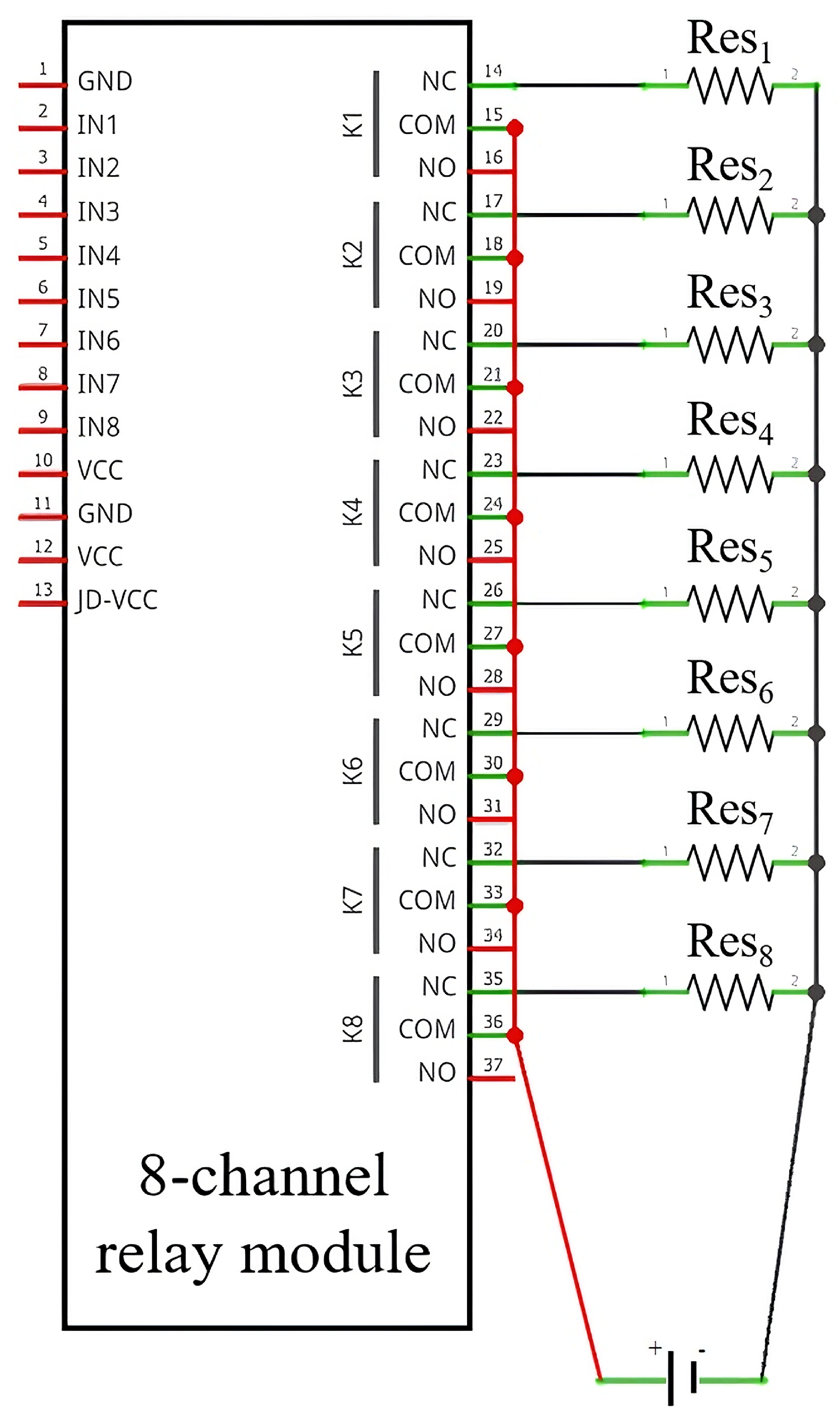
Figure 1 details the connections between the resistors and the relay module channels. Each relay module has three connection pins: common (COM), normally closed (NC), and normally open (NO). Each resistor was connected to the NC pin of the relay module channels, as well as to each other. To establish a parallel association between the resistors, the COM pins of each relay module channel were interconnected. When the channel is activated, the connection between the COM and NC pins is established, while when the channel is deactivated, this connection is broken, and it is the COM-NO connection that becomes energized.

Eight 100 W power resistors with an aluminum shell were utilized, featuring resistances ranging from 100.47 $\Omega$ to 1.15 $\Omega$ (Res1 = 100.47 $\Omega$; Res2 = 47.96 $\Omega$; Res3 = 14.84 $\Omega$; Res4 = 7.80 $\Omega$; Res5 = 4.83 $\Omega$; Res6 = 4.14 $\Omega$; Res7 = 3.50 $\Omega$; Res8 = 1.15 $\Omega$). Therefore, in a scenario where channels 1 and 7 are active, the equivalent resistance provided by the system would be approximately 3.38 $\Omega$. The resistors were connected to the positive terminal of the photovoltaic panel, while the COM pins were linked to the negative terminal.

A 5 V power supply was utilized to energize the relay module, thereby preventing excessive power consumption from the load provided by the Arduino^TM board. A universal USB 5 V cell phone charger was employed to provide power, with the positive terminal connected to the JD-VCC pin and the negative terminal connected to the GND pin.

A voltage divider was used to increase the maximum voltage reading value performed by the Arduino^TM controller, as the controller can only read voltages from 0 V to 5 V, which is done at the analog inputs of the board, with a resolution of 10 bits.

The divider (Figure 2) consists of five resistors with a resistance of 100 k$\Omega$ each. They are arranged into two groups: the first group has three resistors connected in parallel, and the second group has two resistors connected in series. These two groups are then connected in series with each other. In this configuration, the voltage measured across the first group (the parallel one) corresponds to one-seventh of the input voltage. Therefore, the measured voltage must be multiplied by seven, allowing the Arduino^TM to read voltages up to seven times higher than its maximum input range (35 V) for the PV panel tested with output voltage < 25 V.

For current measurements, an ACS712 5 A current sensor was used. The sensor was powered by the Arduino^TM controller via the VCC-5 V connection and grounded via the GND-GND connection. The OUT pin, which provides the current reading of the system, was connected to an analog pin of the controller. The sensor was connected in series with the negative pole of the photovoltaic panel and the voltage divider, enabling the measurement of the current supplied by the panel.

The system sketch can be seen in Figure 3a, while the final assembly can be seen in Figure 3b, in which (A) is the resistor bank, (B) is the 5 V, 10 A relay module with 8 channels, (C) is the Arduino^TM Mega 2560 board, (D) the ACS712 5 A current sensor, (E) the voltage divider, and (F) a 5 V power supply (F). A Dell^TM Latitude D820 computer was used for data storage. All the sketches presented were made using Fritzing 0.9.3b software.

2.2. Logics and Operation of the System

The system’s operating principle involves the switching of resistive loads to which the voltage from the photovoltaic panel is applied, allowing for the acquisition of its characteristic curve. The switching of resistive loads was achieved using an 8-channel relay module and 8 resistors with 100 W power ratings each. Each resistor was individually connected to each channel of the relay module so that when all eight channels were active, all resistors would be associated in parallel. Since the channels can be switched on or off individually, there are two possible states for each resistor, resulting in a total of 2⁸ possible combinations/resistances, which means 256 distinct resistor associations.

Thus, through programming in Arduino^TM, it was possible to vary the equivalent resistance of the resistor association (resistive load) by activating different channels of the relay module at each moment in time, enabling the acquisition of voltage and current values from the photovoltaic panel applied to different resistive loads. To facilitate data acquisition, an LCD shield with a keypad was added to the Arduino^TM module.

Each relay was associated with an index of a binary vector of eight. For each combination among the 256 possibilities, the combination index was converted into binary, consisting of zeros and ones. The binary value was then inserted into the vector, so that when a value equal to 1 is in a certain position of the vector, the relay associated with that position would be active, considering the resistor connected to that relay in obtaining the equivalent resistive load.

Table 2. Truth table of resistor activation and equivalent resistance.

j	Binary	Res1	Res2	Res3	Res4	Res5	Res6	Res7	Res8	${\mathit{R}}_{\mathbf{eq}}$ [$\mathbf{\Omega }$]
0	00000000	0	0	0	0	0	0	0	0	∞
30	00011110	0	0	0	1	1	1	1	0	1.159
44	00101100	0	0	1	0	1	1	0	0	1.938
63	00111111	0	0	1	1	1	1	1	1	0.556
112	01110000	0	1	1	1	0	0	0	0	4.620
217	11011001	1	1	0	1	1	0	0	1	0.809

illustrates representative binary input configurations, indicating which resistors are activated and the resulting equivalent resistance connected to the PV panel.

Each reading from the system provides voltage (V), current (A), and power (W) data from the electric generator. A full sweep of all 256 combinations would take over eight minutes (approx. 501 s), making the measurement highly susceptible to errors from fluctuating solar irradiance and temperature. To address this, 23 combinations were strategically selected to cover the panel’s entire operating range, with increased measurement density near the expected maximum power point (MPP). This ensures that the “knee” of the I–V curve is accurately captured, which is critical for determining the panel’s peak performance, while reducing acquisition time to just 45 s, minimizing the effects of environmental variability.

Notably, the first measurement corresponds to the open-circuit condition, where all relays are deactivated and no current flows, allowing direct acquisition of the open-circuit voltage ($V_{oc}$). Additionally, at lower voltage levels, the output current tends to remain constant and approximately equal to the short-circuit current (I^sc), making it straightforward to infer this parameter even if it is not directly measured through a zero-resistance configuration [39].

These combinations were defined using an 8-bit binary sequence, where each digit (0 or 1) represents whether a specific resistor is switched off or on, respectively. Figure 4 presents the steps for automatically generating the resistive loads and performing voltage and current measurements, while a pseudocode is presented in Appendix A Algorithm A1.

The experimental setup is powered by distinct sources to ensure stable operation. The Arduino Mega 2560 board and the ACS712 current sensor are powered directly via a standard USB connection to a computer, which also facilitates data logging. To prevent overloading the board’s power output, the 8-channel relay module is energized by a separate, dedicated 5V power supply.

The data sampling protocol for each resistive load is executed to ensure measurement stability. The process consists of 10 main reading cycles. In each cycle, the system performs a single voltage reading, followed by a rapid burst of 100 current readings separated by a 100-µs delay. A final 100-ms delay concludes each of the 10 cycles. The average voltage readings and the peak current value (converted to RMS current) were then used to calculate the electrical power delivered by the photovoltaic source. This averaging and sampling strategy results in a total data acquisition time of approximately 1.1 s for each of the 23 data points on the I–V curve, smoothing out noise and rapid fluctuations.

The total system response time to generate a complete I–V curve is 45 s. This duration is a sum of the operations performed for each of the 23 measurement points, which includes 1.1 s for each of the 23 measurement points, a 500 ms delay immediately after the relays are switched, allowing the electrical circuit to stabilize, and a final 300 ms of delay for system pacing and to ensure the relays are fully reset before the next combination is activated.

2.3. System Calibration

To calibrate the voltage measurements, a Minipa^TM ET-2042E digital multimeter was connected in parallel with a commercial photovoltaic panel, which was also connected to the data acquisition system. From the readings of the two devices, the data was regressed to obtain the calibration curve. For the current sensor, the multimeter was connected in series with the photovoltaic panel, which was also connected to the data acquisition system. After one data reading cycle, the current values obtained by the acquisition system were regressed against the current values obtained by the multimeter.

2.4. Experimental Setup

The experimental tests of the data acquisition system were conducted using a commercial Resun^TM RSM060P photovoltaic panel (

Table 3. Specifications of the Resun^™ RSM060P photovoltaic panel.

Parameter	Value	Unit
Output power	$60\pm 3$	W
Efficiency	12.92	%
Maximum Power Voltage	18.54	V
Maximum Power Current	3.36	A
Open Circuit Voltage	22.68	V
Short Circuit Current ($I_{\mathrm{sc}}$)	3.75	A
Nominal Operating Cell Temperature	$45\pm 2$	°C
Temperature Coefficient for Maximum Power	−0.39	%/°C
Operational Temperature	−40 to 85	°C
Number of cells	36	-
Temperature Coefficient for $I_{\mathrm{sc}}$	0.05	%/°C

). The panel was installed on the external metal mezzanine of LabSOLAR’s solar patio, tilted 25° from the horizontal, matching the latitude of Ponta Grossa, PR (25°05′42″ South), and oriented toward geographic north. The panel remained fully exposed to natural environmental conditions, without any modifications or interventions to alter irradiance, wind, or ambient temperature. This ensured that the measurements reflected real operational conditions, with solar irradiance varying naturally throughout the day.

Solar irradiance (G) was measured using a Kipp & Zonen^TM CMP3 pyranometer, positioned with the same inclination and orientation as the photovoltaic panel. Additionally, five (T1, T2, T3, T4 and T5) type-K thermocouples (Omega Engineering^TM) were placed on the back of the PV panel and connected to a Keysight^TM DAQ970A with a 20-channel multiplexer to perform the temperature readings to monitor its temperature. Figure 5 illustrates the setup, showing the positioning of the photovoltaic panel and the pyranometer.

The output of the PV panel was connected to the developed DAQ and measurements of the I–V curve, solar irradiance, and temperature were taken at different times throughout the day to analyze how the PV panel responds to varying operational conditions, such as solar irradiance and operating temperature (T_op), which is the average temperature of the PV panel.

2.5. Experimental Uncertainty

Table 4. Experimental uncertainties.

Parameter	Instrument	Uncertainty
Current	Digital multimeter	$\pm 2\%+0.00001$ A
Current	Data acquisition system	$\pm 2\%+0.00001$ A
Solar Irradiance	Pyranometer	$\pm 3\%$ W/m2
Voltage	Digital multimeter	$\pm 0.5\%+0.01$ V
Voltage	Data acquisition system	$\pm 0.5\%+0.01$ V
Temperature	Type K thermocouple	$\pm 0.25$ °C

shows the uncertainty values considered for each experimental variable described here. For the pyranometer and multimeter, the uncertainty presented in the technical data sheets supplied by the manufacturers was considered. For thermocouples and the resistive load data acquisition system, the uncertainty was considered to be the same as that of the instruments used in their calibration, carried out using the comparative method.

2.6. PV Panel Modeling

Modeling a photovoltaic (PV) panel presents challenges due to its non-linear behavior. Usually, the single and double diode models can be used for this task. Among these, the single diode model strikes an effective balance between complexity and accuracy, with simpler implementation and fewer parameters involved, making it a favorable choice for modeling PV panels in many applications [17,47].

The electrical equivalent circuit of the single diode model is shown in Figure 6. It consists of a diode (D1), which accounts for the non-linearity of the PV panel, a photocurrent source ($I_{ph}$), a series resistance ($R_s$) representing internal losses, and a shunt resistance ($R_{sh}$) modeling leakage currents. Under uniform operating conditions, the voltage ($V_{pv}$) and current ($I_{pv}$) of the PV cells follow the relationship described in Equation (1), in which n is the diode ideality factor, $K_B$ is Boltzmann’s constant ($1.381\times {10}^{-23}$ J/K), $N_s$ is the number of cells, $I_{ph}$ and $I_s$ are the photocurrent and saturation current of the diode, T is the cell temperature in K, and q is the electron charge ($1.602\times {10}^{-19}$ C) [47,48].

$$I_{pv}=I_{ph}-I_s\left(e^{{\displaystyle \frac{q(V_{pv}+I_{pv}{R}_s)}{n{K}_{B}T{N}_s}}}-1\right)-{\displaystyle \frac{V_{pv}+I_{pv}{R}_s}{R_{sh}}}.$$

(1)

The terms $I_{ph}$, $R_{sh}$, and $I_s$ can be modeled mathematically by (2) to (4), respectively, in which G is the solar irradiance (in W/m²), $E_g$ is the band-gap energy with $E_{g,ref}=1.12$ eV for silicon, $K_i$ is the temperature coefficient of short circuit current, and $I_{ph,ref}$ and $R_{sh,ref}$ are the photocurrent and shunt resistance at standard test conditions (1000 W/m² and 298.15 K) [47].

$$I_{ph}=I_{ph,ref}+K_i(T-T_{ref}){\displaystyle \frac{G}{1000}},$$

(2)

$$R_{sh}=R_{sh,ref}{\displaystyle \frac{1000}{G}},$$

(3)

$$I_s=I_{s,ref}{\left({\displaystyle \frac{T}{T_{ref}}}\right)}^3\exp \left[{\displaystyle \frac{q{E}_g}{K_B}}\left({\displaystyle \frac{1}{T_{ref}}}-{\displaystyle \frac{1}{T}}\right)\right].$$

(4)

Examining (1) to (4), five key parameters must be identified to accurately model the I–V curve of the PV panel: $I_{ph,ref}$, $R_{sh,ref}$, n, $I_{s,ref}$, and $R_s$. These parameters were determined using the differential evolution (DE) global optimization algorithm, implemented via the differential_evolution function in the SciPy library (v1.15.3). The algorithm was run with the following settings: population size = 15 × number of parameters, mutation factor = (0.5, 1), crossover probability = 0.7, and stopping tolerance = 0.01. The initialization was performed via Latin hypercube sampling (init = latinhypercube) to ensure a wide search space. The algorithm ran for up to 1000 generations (maxiter = 1000) and used the best1bin strategy for mutation.

Optimization was constrained using physically plausible bounds for each parameter, as presented in

Table 5. Comparison of parameter bounds used in this work with values reported in the literature.

Source	${\mathit{I}}_{\mathbf{ph},\mathbf{ref}}$ [A]	${\mathit{I}}_{\mathbf{s},\mathbf{ref}}$ [A]	n [-]	${\mathit{R}}_{\mathit{s}}$ [$\mathbf{\Omega }$]	${\mathit{R}}_{\mathbf{sh},\mathbf{ref}}$ [$\mathbf{\Omega }$]	Notes
[49]	0.7608	$3.23\times {10}^{-7}$	1.4812	0.03638	53.72	Monocrystalline
[50]	4.7103	$1.48\times {10}^{-5}$	1.3410	0.8020	364.51	Polycrystalline
[50]	4.7063	$8.32\times {10}^{-4}$	1.3110	0.1620	121.31	Monocrystalline
[47]	8.2288	$2.32\times {10}^{-10}$	0.9774	0.3448	150.69	Multicrystalline
[51]	5.44	$1.41\times {10}^{-4}$	1.96	0.0024	6.66	Double single-diode model
[51]	4.31	$8.88\times {10}^{-5}$	1.93	0.0025	27.81	Double single-diode model
[51]	5.22	$1.30\times {10}^{-4}$	1.92	0.0025	16.11	Double single-diode model
[51]	4.88	$5.84\times {10}^{-5}$	1.84	0.0029	6.53	Double single-diode model
This study (bounds)	[0, 10]	$[{10}^{-12},{10}^{-8}]$	[0.5, 2.0]	[0.01, 1.0]	[100, 300]	Used for optimization

, and defined based on previous results reported in the literature. All other algorithmic parameters were kept at their default values using the differential_evolution function from the SciPy library. These settings proved sufficient for the algorithm to converge to a stable solution with minimal error.

Table 5 also highlights the importance of the individual calibration of model parameters, since different PV panel technologies (e.g., monocrystalline, polycrystalline, and multicrystalline) exhibit significant variation in electrical characteristics. This variability reflects differences in material properties, manufacturing processes, and aging effects, all of which influence the I–V curve shape and, consequently, the values of single-diode model parameters.

While the bounds defined in this study proved adequate to capture the behavior of the tested panel, they may not be universally applicable to all PV technologies or environmental conditions. Therefore, the re-optimization of model parameters is recommended when characterizing different modules or deploying the system under markedly different irradiance and temperature profiles. Fortunately, the use of a robust global optimization algorithm (differential_evolution) allows for efficient re-fitting with minimal user intervention, which supports the practical application of this approach in both laboratory and field scenarios.

3. Results

This section describes the main results of the study, including sensor calibration, model optimization, and PV panel behavior.

3.1. Sensor Calibration

As can be seen from Figure 7a,b, both regressions were linear in nature with an R² determination coefficient close to 1, which indicates a strong correlation among the data analyzed. Since the calibration was carried out using the comparative method, the uncertainty of the data acquisition system was the same as that of the digital multimeter, which was $\pm 2\%+0.00001$ A for the current, and $\pm 0.5\%+0.01$ V for the voltage.

To ensure the sustained accuracy and reliability of the data acquisition system over time, we recommend implementing a schedule for periodic recalibration. As a best practice for field instrumentation, this procedure should be conducted annually, or more frequently if the system is deployed in harsh thermal environments. Recalibration involves repeating the initial validation process, where the DAQ’s measurements are compared against a certified reference multimeter, to compensate for any measurement drift arising from the long-term effects of component aging and thermal cycling.

3.2. PV Modeling

Equations (1) to (4), along with the data from Table 3, were implemented in a Python 3.11.1 environment, where the optimization algorithm was used to fit the parameters to an I–V curve provided by the manufacturer under standard test conditions. The optimized values obtained were $I_{ph,ref}=3.8330$ A, $R_{sh,ref}=92.7474\Omega$, $n=0.99996$, $I_{s,ref}=8.22073\times {10}^{-11}$ A, and $R_s=0.23147\Omega$.

Figure 8 compares the manufacturer’s data at standard conditions with the optimized model, showing agreement between data for the current (I) and output power (P), with a mean average percentage error (MAPE) of 4.40% for the current (I) values.

With the optimization of these five parameters, (1) to (4) can be implemented along with the data from Table 3. The experimental measurements obtained with the proposed data acquisition system (DAQ) can be compared with the results obtained from the single-diode model.

3.3. Main Results

Table 6. Results from the data acquisition system.

Time	Index	Resistive Load [$\mathbf{\Omega }$]	Voltage [V]	Current [A]	Power [W]
14:02:06	0	∞ *	20.6	0.0	0.0
14:02:08	1	100.4	20.5	0.3	5.6
14:02:10	2	48.0	20.4	0.4	9.1
14:02:12	3	32.5	20.0	0.7	13.3
14:02:14	4	14.8	19.7	1.3	26.1
14:02:16	5	12.9	19.4	1.5	29.8
14:02:18	6	11.3	19.3	1.7	33.2
14:02:20	7	10.2	19.2	1.9	36.2
14:02:22	8	7.8	18.5	2.4	45.4
14:02:24	9	7.2	18.3	2.6	47.9
14:02:26	10	6.7	18.2	2.8	50.2
14:02:28	12	5.1	17.1	3.3	56.9
14:02:30	15	4.4	15.8	3.6	56.9
14:02:32	19	4.2	15.1	3.7	55.9
14:02:34	24	3.0	11.1	3.8	41.9
14:02:36	31	2.3	8.9	3.8	33.8
14:02:38	41	2.6	10.2	3.8	38.7
14:02:41	55	1.8	7.2	3.8	27.6
14:02:43	74	2.3	8.7	3.8	33.1
14:02:45	100	1.7	6.4	3.8	24.5
14:02:47	136	1.0	3.8	3.8	14.5
14:02:49	185	0.7	2.8	3.8	10.6
14:02:51	252	0.6	2.4	3.8	9.2

* Open circuit voltage with all relays deactivated.

illustrates the data obtained from the photovoltaic panel in one complete reading sweep using the resistive load data acquisition system. The first measurement was taken with all relay module channels turned off, meaning the photovoltaic panel was in an open-circuit condition. Subsequent measurements were taken using different resistor combinations from the resistor bank. The entire data acquisition process takes 45 s and successfully automates the switching of the load applied to the PV panel. Readings were taken at 30 min intervals between 9:00 a.m. and 4:00 p.m., totaling 15 measurements. The analysis presented in this paper is based on the data collected during this single day of operation.

The data shown in Table 6 illustrates the importance of using a system to apply loads to electric generators, since the power generated varies according to the load applied, and it is necessary to obtain the device’s maximum power value to determine its efficiency. Another advantage of the system is that the time of each acquisition is recorded, allowing the efficiency of the device to be calculated correctly from the solar irradiance value collected at the same time as the maximum power acquisition.

It is important to note that of the 256 possible associations, only 23 were selected to reduce the measurement time. If all 256 possibilities were carried out, it is estimated that the data collection time would go from 45 s to approximately 501 s. The first measurement (Index 0 from Table 6) corresponds to the open-circuit voltage of the PV panel.

Furthermore, as can be seen in As in Figure 9a, depending on the conditions to which the generator is subjected, in this case, a photovoltaic panel subjected to different solar irradiance values (G) and operational temperatures (T_op), the maximum power value can be obtained with different resistive loads. It can also be observed that the range of resistive load values applied to the photovoltaic panel was sufficient to achieve the maximum power value even under varying solar irradiance conditions.

The data acquisition system was also able to observe the characteristic curve of the photovoltaic panel under the incidence of different average levels of solar irradiance, as can be seen in Figure 9b. Even though these results were not obtained under controlled temperature and solar irradiance conditions, the behavior shown is very similar to what is expected for these devices, in which higher solar irradiance values tend to increase the voltage and current values of the photovoltaic panel, with the most significant increase being in the current, which consequently increases its power.

Figure 9b also shows the comparison between the DAQ and model data for the I–V curves and output power for each G and T_op condition. It can be seen that, in general, the model was able to predict the same behavior for the I–V and output power curves; however, there were some difference in absolute values compared to the measurements from the DAQ.

Figure 10a,b illustrate the importance of acquiring data quickly. When operating the device under ambient conditions, it is exposed to variations in solar irradiance. Figure 10a shows the panel’s characteristic curve obtained from an acquisition made with constant solar irradiance, while Figure 10b shows the acquisition with variations in solar irradiance. If the acquisition is done slowly, the likelihood of the panel being exposed to different G conditions is greater, making it more difficult to characterize the device.

Figure 11a,b show the MAPE between the DAQ and model data for the I–V and output power curves, reaching values below 20%, but higher than the MAPE obtained during the optimization of the standard conditions parameters.

This may occur because the values of temperature and solar irradiance may not be constant along the whole PV panel, as

Table 7. Temperature and solar irradiance measurements.

G [W/m2]	${\mathit{\sigma }}_{\mathit{G}}$ [W/m2]	T1 [°C]	T2 [°C]	T3 [°C]	T4 [°C]	T5 [°C]	${\mathit{\sigma }}_{\mathit{T}}$ [°C]
914.26	1.11	48.73	46.16	46.05	52.02	53.08	2.84
914.08		49.41	47.48	46.52	52.40	53.40	2.76
914.27		49.49	47.64	46.81	52.52	53.35	2.73
914.68		48.27	46.23	46.23	52.18	53.01	2.55
915.55		47.14	45.87	45.66	51.75	52.64	2.47
914.88		46.96	45.68	45.50	51.65	52.57	2.44
914.26		47.57	46.13	45.58	51.53	52.70	2.43
913.44		47.56	46.41	45.64	50.82	52.43	2.41
912.82		47.40	46.08	45.41	50.47	52.30	2.46
912.20		47.60	46.28	45.83	50.45	52.39	2.40
912.07		47.47	46.49	45.98	50.91	52.40	2.42

shows. To be able to compare the model with the experimental data, average temperature and irradiance values were used, so this high MAPE between the DAQ and model data may occur due the fact that in the optimization process, the experimental data used as reference was obtained at constant operational temperature and solar irradiance, conditions that are not feasible in a real operation.

The data in Table 7 reveals a significant thermal gradient across the panel’s surface, with a temperature standard deviation reaching up to 2.84 °C. This indicates that different cells on the panel were operating at notably different temperatures. A single-diode model, which relies on a single average operating temperature, cannot fully capture the complex effects of this non-uniformity on the panel’s real-world behavior.

Similarly, the use of a single pyranometer in the experimental setup assumes that solar irradiance is uniform across the entire panel area. In practice, factors such as localized soiling or the passing shadows of clouds can create uneven illumination, causing some cells to generate less current than others. This electrical mismatch also affects the overall I–V curve in a way that a model using a single irradiance value (G) cannot predict.

These simplifications (using an average temperature and a single-point irradiance measurement) are key sources of the observed error between the model and the experimental data. Therefore, to further enhance model performance in future work, deploying multiple pyranometers to better map the irradiance distribution could provide a more accurate input for the model. This highlights the limitations of idealized models and reinforces the necessity of empirical field data to develop more robust and predictive simulations.

This issue resulted in an overestimation of the output power and energy efficiency ($\eta$) by the model, especially for lower values of G (relative difference of approx. 27% for G = 246.33 W/m²), as

Table 8. Maximum output power and efficiency.

G [W/m2]	Top [°C]	Pmax,DAQ [W]	Pmax,model [W]	${\mathit{\eta }}_{\mathit{DAQ}}$	${\mathit{\eta }}_{\mathit{model}}$
913.86	48.91	51.70	53.05	13.19	13.54
827.59	49.00	42.72	48.53	12.04	13.67
615.45	44.21	33.13	35.98	12.55	13.63
488.90	42.80	26.45	29.18	12.62	13.92
246.33	36.64	11.01	13.98	10.42	13.23

shows. Using the experimental results obtained with the DAQ to optimize the model parameters can reduce this average difference in the model results.

Using the experimental results for $G=615.45$ W/m², the optimized values obtained were $I_{\mathrm{ph},\mathrm{ref}}=3.4694$ A, $R_{\mathrm{sh},\mathrm{ref}}=244.2973\Omega$, $n=0.95688$, $I_{\mathrm{s},\mathrm{ref}}=2.92672\times {10}^{-11}$ A, and $R_s=0.5809\Omega$.

Figure 12a,b shows the results of using these new optimized parameters. The MAPE of the I–V curves and output power curves reduced from 18.23 and 18.54% to 7.06 and 7.22%, respectively, and the relative difference between the panel efficiency reduced from around 27% to around 15%.

Table 9. Comparison of validation metrics before and after model re-optimization.

G [W/m2]	${\mathit{R}}^2$ (Current)		RMSE (Current) [A]		${\mathit{R}}^2$ (Power)		RMSE (Power) [W]
	Before	After	Before	After	Before	After	Before	After
913.86	0.9655	0.9646	0.2152	0.2178	0.9364	0.9686	4.0370	2.8360
827.59	0.9174	0.9976	0.2888	0.0495	0.8951	0.9959	4.5018	0.8847
615.45	0.9067	0.9995	0.2121	0.0157	0.9259	0.9993	2.9093	0.2860
488.90	0.8718	0.9910	0.1858	0.0494	0.9219	0.9879	2.3197	0.9147
246.33	0.5178	0.8932	0.1398	0.0658	0.8467	0.9366	1.2502	0.8039

presents a comparative analysis of the model’s performance before and after parameter re-optimization using Differential Evolution. Notably, all metrics exhibit substantial improvement following re-optimization, particularly in irradiance levels below 700 W/m², where initial accuracy was lower. For instance, at 827.59 W/m², the RMSE for current dropped from 0.2888 A to 0.0495 A, and the $R^2$ for power increased from 0.8951 to 0.9959. Similarly, for the lowest irradiance level (246.33 W/m²), $R^2$ improved from 0.5178 to 0.8932 for current, indicating a much better model fit. These improvements reinforce the importance of tailored parameter calibration under varying field conditions to enhance model reliability.

These results show the importance of the development and use of a data acquisition system that can perform a voltage sweep on the PV module to obtain the I–V curves in real conditions of operation. These valuable data can be used both to compare different operational conditions and to obtain real-time data to optimize PV panel models.

The comparison in

Table 10. Comparison between the proposed Arduino-based I–V tracer and commercial systems.

Feature	Arduino-Based	HT I–V500w [8]	Solmetric PVA-1500 [52]
Voltage Range [V]	0–35	15–1000	20–1500
Current Range [A]	up to 5	0.1–15	up to 30
Voltage Accuracy	$\pm 0.5\%+0.01$	±0.5% rdg + 2 dgt	±0.5% + 0.25
Current Accuracy	$\pm 2\%+0.00001$	±1.0% rdg + 2 dgt	±0.5% + 0.04
Power Accuracy	±4%	±1.0% rdg + 6 dgt	±1.7% + 1.0 W
Full Sweep Time [s]	∼45	5	0.05–2
Irradiance/Temp Sensor	External	Yes	Yes (SolSensor)
IoT/Automation	Manual (expandable to ESP32/Wi-Fi)	USB + SW	Wi-Fi + SW
Estimated Cost [USD]	<100 US $	2 k–4 k+	10 k+

highlights the performance and trade-offs of the proposed Arduino-based I–V tracer relative to three widely used commercial systems. While the commercial instruments deliver higher accuracy, faster acquisition times, and comprehensive automation, their high cost and proprietary architecture limit accessibility, particularly in educational, low-resource, or off-grid contexts.

In contrast, the proposed system offers a low-cost, open-source alternative with sufficient resolution to capture the critical features of a PV panel’s performance curve, including the maximum power point. Its portability, simplicity, and transparency make it an ideal platform for teaching photovoltaic concepts, prototyping control algorithms, or enabling low-cost diagnostics in decentralized energy applications. This underscores the educational and practical value of developing open-hardware tools for renewable energy research and training.

4. Conclusions

This study introduces a low-cost, Arduino^TM-based data acquisition (DAQ) system that overcomes key limitations of existing methods by integrating automated resistive load control and rapid data acquisition in a single setup. Unlike traditional systems that require manual adjustments, this system can automatically vary the resistive load and acquire real-time data, which is crucial for accurate PV panel characterization, especially in field conditions where environmental factors such as solar irradiance and temperature can fluctuate. The data acquisition time of 45 s minimizes the impact of these variables.

The single-diode model provided good results under standard conditions (manufacturer’s data—MAPE of 4.40% for current values). However, discrepancies arose under real operational conditions, particularly at lower solar irradiance levels (with a relative difference of about 27% at G = 246.33W/m²). This highlights the importance of real-time experimental data for optimizing PV models, as standard laboratory conditions may not reflect actual field performance. When experimental data were used to optimize the model, the accuracy improved, reducing the MAPE for I–V curves and output power from 18.23% and 18.54% to 7.06% and 7.22%, respectively.

The proposed system offers a cost-effective and flexible alternative to commercial I–V curve tracers, making it especially valuable for educational institutions, small-scale renewable energy projects, and researchers in developing countries. Its open-source hardware and software design ensures that it can be easily replicated and adapted to meet various experimental needs, further enhancing its accessibility.

Future Work

A promising extension of the proposed system involves its integration with a microcontroller like the ESP32, which provides built-in Wi-Fi and Bluetooth capabilities. The transition would be straightforward, as the ESP32 is compatible with the Arduino IDE, allowing the core logic to be easily ported. This upgrade would enable real-time data transmission to cloud-based IoT platforms capable of executing adaptive algorithms. These algorithms could adjust the model parameters dynamically, in response to changing environmental conditions such as irradiance and temperature. Such an approach would not only improve the accuracy of PV panel modeling but also enable on-the-fly diagnostics and fault detection, enhancing the system’s applicability for long-term monitoring and smart grid integration.

The programmable resistive load can be used as a cost-effective platform to develop and validate Maximum Power Point Tracking (MPPT) algorithms. Instead of a simple sweep, the microcontroller could execute different MPPT strategies (such as perturb and observe, incremental conductance, or particle swarm optimization) by dynamically changing the load to actively track the panel’s maximum power point. This allows for direct, empirical benchmarking of algorithm efficiency under real-world conditions.

Also, by integrating electronic multiplexers or relay-based switching matrices at the input, the system can be extended to sequentially characterize multiple PV panels in an array. The microcontroller would first select a panel, perform the I–V trace, store the data, and then switch to the next panel. This automated process is invaluable for identifying module mismatch, localized faults, or degradation across an entire PV string in both laboratory and educational settings where cost-effective scalability is essential.