The Influence of Hard Protection Structures on Shoreline Evolution in Riohacha, Colombia

Abstract

Over the past 50 years, coastal erosion has become an increasingly critical issue worldwide, and Colombia’s Caribbean coast is no exception. In urban areas, this challenge is further complicated by hard protection structures, which, while often implemented as immediate solutions, can disrupt sediment transport and trigger unintended long-term consequences. This study examines shoreline changes in Riohacha, the capital of La Guajira Department, over a 35-year period (1987–2022), focusing on the impacts of coastal protection structures—specifically, the construction of seven groins and a seawall between 2006 and 2009—on coastal dynamics. Using twelve images (photographs and satellite) and the Digital Shoreline Analysis System (DSAS), the evolution of both beaches and cliffs has been analyzed. The results reveal a dramatic shift in shoreline behavior: erosion rates of approximately 0.5 m/year prior to the interventions transitioned to accretion rates of up to 11 m/year within the groin field, where rapid infill occurred. However, this sediment retention has exacerbated erosion in downstream cliff areas, with retreat rates reaching 1.8 ± 0.2 m/year. To anticipate future coastal evolution, predictive models were applied through 2045, providing insights into potential risks for infrastructure and urban development. These findings highlight the need for a strategic, long-term approach to coastal management that considers both the benefits and unintended consequences of engineering interventions.

1. Introduction

The shoreline serves as the boundary between land and sea, subject to alterations from both natural processes and anthropogenic factors. Natural processes can be associated with the usual coastal dynamics (e.g., waves, tides, sediment transport), more extreme phenomena (such as storms or floods), and factors related to the terrestrial part (such as vegetation, geology, cliff profile, etc.). In addition, these natural processes are being modified in many cases by the effects of climate change (i.e., sea level change or extreme events), especially in the last 40/50 years [1]. These factors have altered natural coastal dynamics, leading to localized erosion and deposition processes that have transformed the original state of certain areas [2]. Anthropogenic factors can also determine or condition coastal evolution with the construction of coastal engineering infrastructures, sand extraction, land use, etc. All these phenomena, together or separately, can modify the erosion of cliffs and beaches [3,4]. The problems associated with erosional phenomena range from increased exposure of the population to natural hazards such as tsunamis or floods, to the degradation of ecosystems, or economic losses due to the destruction of houses, the decline in tourism, or the loss of land itself [5,6]. In contrast, accretion zones are generally less vulnerable to natural hazards by moving the coastline further offshore; in addition, tourism and economic activity tend to increase [7].

Latin America’s coastal zones face growing climate challenges, including erosion, rising vulnerability, and ecosystem degradation. With over 600 million inhabitants, many countries—such as Brazil, Colombia, and Venezuela—have more than 30% of their population in Low-Elevation Coastal Zones (LECZs), areas below 10 m above sea level [8]. These regions are particularly vulnerable to flooding, sea level rise, tsunamis (and the resulting inundation), and other extreme weather events [1,9,10]. Additionally, Latin America is projected to experience the second-largest population growth globally, with an 80% increase in LECZ residents over the next century [11]. Colombia’s coastal regions, particularly the Caribbean coast, are renowned for their diverse marine ecosystems and pristine beaches, which support a thriving tourism industry and play a key role in the national economy [12]. However, these areas are undergoing profound transformations due to coastal erosion, sedimentation, and human interventions such as dam construction, inadequate coastal infrastructure, and mangrove deforestation. Increased tourism has further intensified these pressures. Currently, approximately 50% of the Colombian Caribbean coastline is affected by erosion, leading to the displacement of some coastal communities [13]. Studies report varying erosion rates from the 1950s to the early 2010s across different regions: from 0.62 m/yr to 3.3 m/yr in the Department of Córdoba, up to 5.3 m/yr in Magdalena, and around 3 m/yr in La Guajira [14,15,16].

The study of shoreline evolution is essential for assessing coastal risks and informing sustainable management strategies [17]. To accurately measure shoreline changes, various remote sensing techniques and analytical tools are employed, including aerial photographs, satellite imagery, historical maps, and airborne LiDAR surveys. These, combined with Geographic Information Systems (GIS), enable the reconstruction of coastline evolution across different temporal scales [18]. Such datasets provide critical insights into both long-term (>60 years) and medium-term (10–60 years) shoreline movements and transformations [19]. Recent studies demonstrate the effectiveness of these methodologies. In a broader historical approach, Castedo et al. [20] analyzed Holderness Coast (U.K.) cliffs through map data (1852–1929), aerial photos (1952–1996), and LiDAR-GPS data (2011), reporting an average recession rate of 1.25 m/yr. Similarly, Ponte Lira et al. [21] examined the evolution of 12 shore platform beaches along the Cascais coast, Portugal, using Digital RGB orthophoto maps. Leisner et al. [22] integrated satellite imagery with UAV-based photogrammetry to assess beach-cliff erosion at Pacheco Beach, Brazil. Yadav et al. [23] used Landsat-8 imagery and automatic shoreline extraction to analyze anthropogenic impacts on the Maravanthe Coast, India, revealing an 8% decrease in erosion zones and a 7% increase in accretion zones.

Beyond natural processes, human interventions—such as coastal protection structures—play a key role in shoreline evolution. Hard engineering solutions like seawalls, groins, and breakwaters are often implemented to mitigate erosion, but they can significantly alter sediment dynamics. While these structures may stabilize targeted areas, they often induce downdrift erosion, disrupt natural sediment transport, and modify deposition patterns, leading to unintended consequences for adjacent coastal systems [24]. As a result, historical data and predictive modeling are essential for forecasting future shoreline changes and adapting coastal management strategies accordingly [25]. Numerous models of varying complexity have been developed to estimate and predict coastal erosion, helping to project shoreline positions and assess risks. Among these, key approaches include the Bruun rule [26], the Kalman filter method [27,28], historical data extrapolation [20], the Coastal Evolution Model (CEM) [29], XBeach [30], and the Generalized Model for Simulating Shoreline Change (GENESIS) [31]. These models can be applied individually or in combination, depending on the specific coastal environment, data availability, and study scale. Integrating multiple models and validating them with field data enhances the accuracy and reliability of coastal change predictions.

This study investigates coastal development in the urban area of Riohacha, the capital of La Guajira Department on the Colombian Caribbean coast. Although research on shoreline dynamics and erosion modeling has advanced considerably in recent years, few studies have applied a combination of predictive modeling approaches in the Caribbean context, particularly in medium-sized urban areas with significant geomorphological heterogeneity and infrastructure pressures. This lack of integrated modeling applications limits the ability to assess future coastal risks with higher confidence. The present study addresses this gap by applying and comparing three modeling techniques—HTA, EHD, and KFB—along a representative coastal segment of the Colombian Caribbean. It aims to analyze the potential correlation between the construction of seven groins and the resulting coastal changes, specifically the growth of the coastline where the structures are located and the erosion observed in the southern cliff zone. The primary hypothesis is that the groins have contributed to the stabilization and accretion of the coastline near the structures, while inducing erosion further south, leading to a cause-and-effect relationship between human intervention and coastal response. For this purpose, the images available before (1987–2006) and after (2009–2022) the anthropic interventions have been rectified, profiled, and analyzed. The work includes the statistical analysis of the evolution of coastlines; the calculation of modified surfaces; and the application of predictive models (up to 2045) that should serve as a basis for future land management, providing a point of support for decision making in any coastal region.

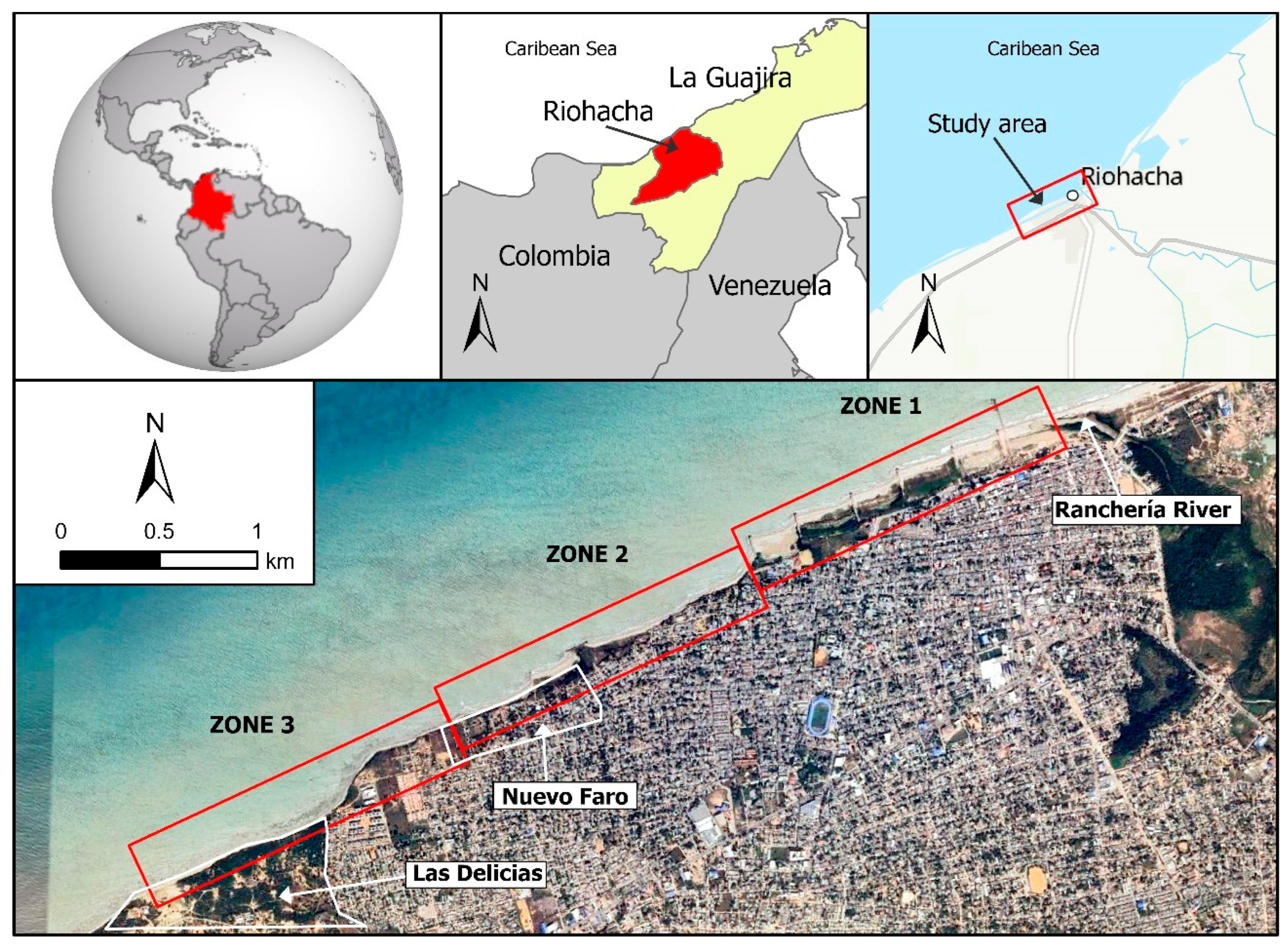
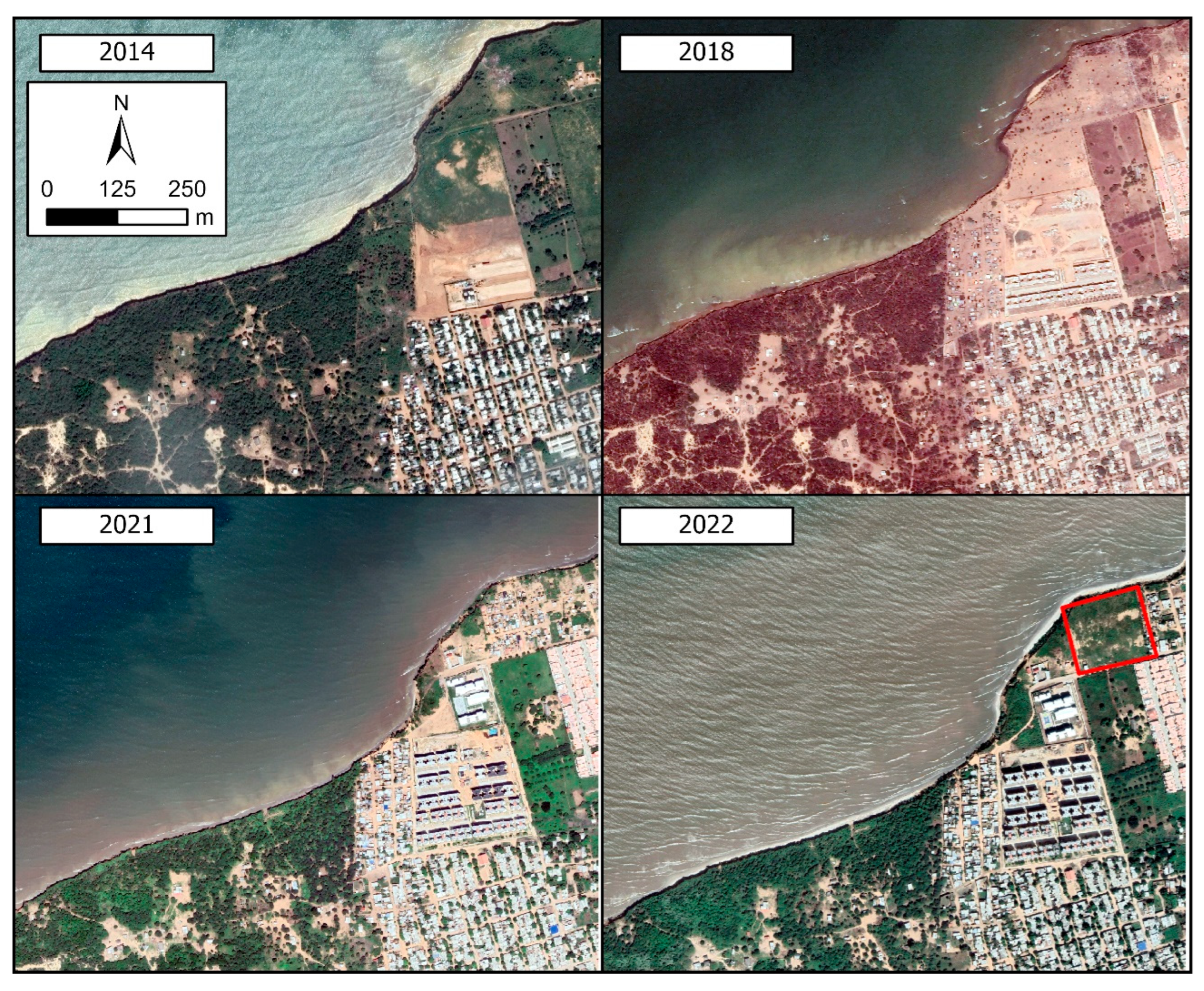
2. Study Area and Geographical Data

The Colombian Caribbean coastline spans from the eastern border with Venezuela to the western border with Panama, primarily oriented in a NE–SW direction, with occasional segments aligning W–E (Figure 1). La Guajira peninsula is a complex region, where different Quaternary interactions (i.e., climate conditions, human intervention, tectonics) have defined the current geomorphology [32]. The entire area is a set of Jurassic to Tertiary tectonically uplifted blocks of granitic, metamorphic, and sedimentary rocks adjacent to sedimentary basins filled with Tertiary sediments [33]. Therefore, the landscape units include mountainous areas and extensive deltaic plains. The coastal morphology of the Peninsula, shaped mainly by marine conditions and coastal processes typical of tropical climates, is characterized by numerous bars and medium sandy beaches along elongated coastal plains, bays, and cliffs [33,34].

In the Colombian Caribbean, tidal patterns are mixed semidiurnal and micromareal, with average amplitudes around 0.3 m and peak values up to 0.65 m [35,36]. The dominant swell, influenced by climatological factors, comes from the NE-SW direction from November to July, with wave heights reaching 4.5 to 5 m [37,38]. In the remaining months, swell direction becomes more variable, shifting to a SW-NE orientation, with wave heights under 1.5 m. During specific meteorological conditions, southerly winds generate short-duration, high-frequency waves, which can lead to significant erosion. Sea level rise in the Colombian Caribbean (based on data from the Cartagena station south of Riohacha) has shown a slight oscillation from 1950 to 2015, with rates ranging from 5.5 mm/year [16,38] to 5.9 mm/year [39]. Projections for sea level rise by 2050 (starting from 2020) estimate an increase of 24–26 cm under moderate (Representative Concentration Pathway—4.5) or no reduction scenarios (RCP 8.5) [40]. Historically, sediment influx in the region came from the Sinú and Ranchería rivers, but damming of these rivers in the 1990s and mid-2000s altered sediment transport [41], shifting the main source to wind-driven processes from the upper Guajira region, with occasional reversals during heavy precipitation [42].

The city of Riohacha, located in the central part of La Guajira Department, has 46 km of coastline, approximately 7% of the Department [37]. The city, home to over 250,000 residents, relies primarily on tourism as its main economic activity. Previous studies have documented a long-standing pattern of beach erosion in the northern sector of the city, particularly near the mouth of the Ranchería River [37,43]. To mitigate these effects, six groins were built at the end of 2007 along the 1.5 km waterfront of Riohacha city (Figure 2A). These groins measure 150 m in length, 13 m in width, and stand 6 m high, spaced at an average interval of 250 m [15]. Additionally, a seawall was constructed (Figure 2B).

The Riohacha area is underlain by the Monguí Formation [44], composed of Paleogene and Neogene sandy claystones and semi-consolidated conglomerates with igneous pebbles [45]. This formation outcrops near the Ranchería River mouth but is covered southward by Quaternary sediments, mainly alluvial deposits from perennial rivers and streams. In the central and southern part of the city (Figure 2B,C), small beach deposits overlap these alluvial sediments, consisting of semi-consolidated sandy clays and plastic clays rich in ferromagnesian minerals and oxides from the Sierra Nevada de Santa Marta [46,47].

Finally, the study focuses on a 5 km stretch of coastline between the mouth of the Ranchería River (north) and the indigenous reservation Las Delicias (south) (Figure 1). The area is divided into three sections (Figure 2):

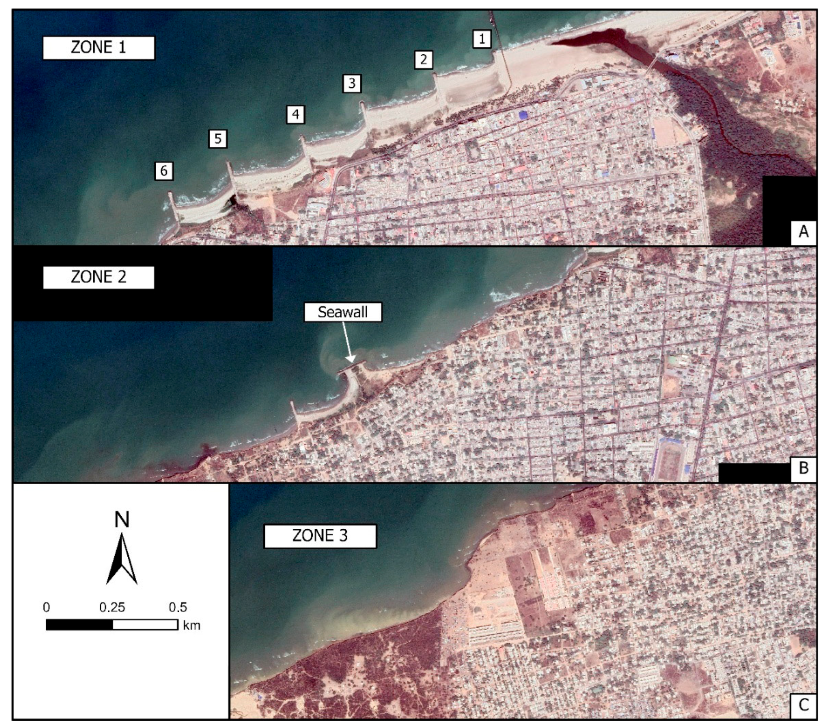
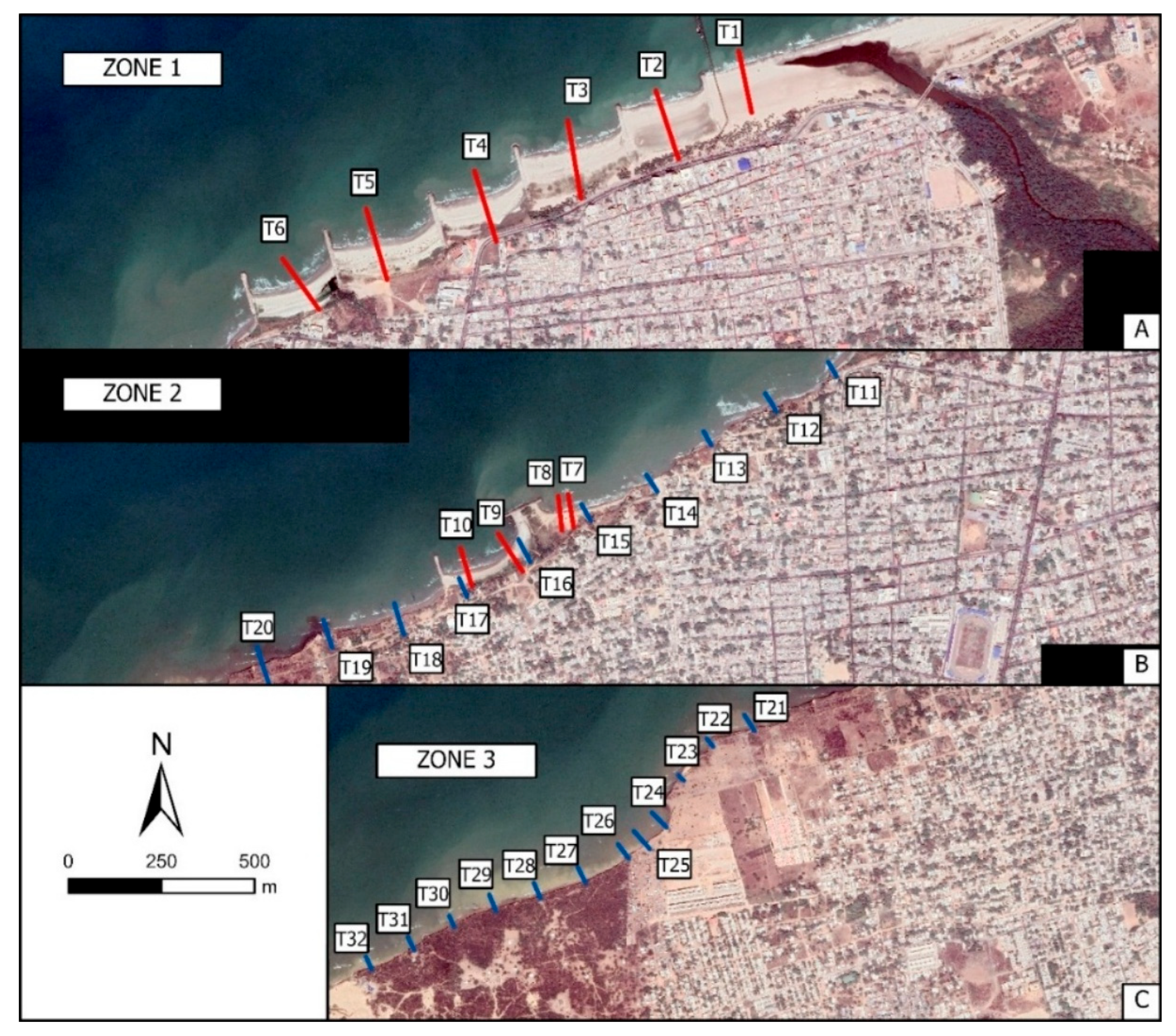
• Zone 1 (1450 m) extends from the river mouth to groin 6, encompassing the groin field and featuring well-developed beaches.
• Zone 2 (1900 m) stretches from groin 6 to the Nuevo Faro neighborhood. This section includes a small cliff (~6.5 m high) with narrow beaches at its base.
• Zone 3 (1600 m) runs from a coastal rocky outcrop to Las Delicias. Here, the cliffs are slightly higher (~9.1 m) with no beach at the base, except in the southern area.

3. Methodology

The methodological workflow followed in this research includes the following: (1) image acquisition; (2) georeferencing (using ArcGIS Pro); (3) shoreline profiling (using ArcGIS Pro); (4) data extraction with the use of Digital Shoreline Analysis System (DSAS) [48] and change in the surface area; and (5) future trends in shoreline change.

To conduct this research, twelve images were obtained from two sources: (i) aerial photographs from 1987 and 1997 provided by the Instituto Geográfico Agustín Codazzi (IGAC) [49] and (ii) ten satellite images from Google Earth [50].

Table 1. Main information from the images used in this research.

Image	Source	Date
IGAC1987	Instituto Geográfico Agustín Codazzi	14 September 1987
IGAC1997	Instituto Geográfico Agustín Codazzi	12 January 1997
GE2003-02	Google Earth	February 2003
GE2006-03	Google Earth	March 2006
GE2009-10	Google Earth	October 2009
GE2011-01	Google Earth	January 2011
GE2013-02	Google Earth	February 2013
GE2014-11	Google Earth	November 2014
GE2018-03	Google Earth	March 2018
GE2019-10	Google Earth	October 2019
GE2020-10	Google Earth	October 2020
GE2022-11	Google Earth	November 2022

details the images and their acquisition dates. For consistency in the analysis, all images were georeferenced using common control points, with the November 2022 image serving as the reference. The 1987 photographs were individually rectified, while the 1997 images were processed into an orthomosaic using Agisoft Metashape [51] and IGAC-provided projection center coordinates. The reference system used for georeferencing was “MAGNA-SIRGAS/Riohacha urban grid EPSG:6267.”

After uploading the 12 orthophoto mosaics covering all study years into the GIS, the next step involved manually digitizing the shorelines and cliff tops [20]. Manual delineation was chosen over automated remote sensing methods [52], as the relatively small study area ensures greater accuracy through manual tracing. Although manual digitization improves precision in heterogeneous environments and allows for expert interpretation of complex features, it is not free from limitations. This approach may introduce a degree of subjectivity, and reproducibility can be affected by inter-operator variability. To maintain consistency in the identification of geomorphological features, all delineation tasks were carried out by a single operator. In this study, although no repeated digitization or formal cross-validation was conducted, the operator applied expert visual criteria, and each delineation was carefully reviewed within the GIS environment to ensure topological coherence and alignment with identifiable geomorphological features. Shoreline mapping was based on the most recent wet tide mark visible in the orthophotos, marking the boundary with the backshore [3,53], a method well-suited for sedimentary coasts exposed to open-sea dynamics. Similarly, the cliff top was delineated by identifying the visually distinguishable crest of the slope [54].

The DSAS v5.1 was used to statistically analyze the historical evolution of both the shoreline and the cliff [48]. The DSAS workflow consists of three key steps: defining a baseline, generating transects (profiles), and calculating change rates [55]. The shorelines and cliffs for each zone were stored in a shapefile within a personal geodatabase, with each feature attributed to a date in MM/DD/YYYY format. The oldest available shoreline (IGAC1987 in Table 1) was selected as the baseline. Transects were generated perpendicular to the coastline at regular intervals, allowing DSAS to detect intersections with shorelines from different years. These intersections provided a series of position-date points, forming the basis for analyzing coastal evolution. Using DSAS, the primary metric obtained is the Net Shoreline Movement (NSM), which represents the maximum displacement along each transect between the earliest and most recent shoreline or cliff position, measured in meters. Additionally, DSAS applies to a linear regression model fitted by least squares to analyze shoreline or cliff evolution over time, providing key parameters for predictive modeling. The Linear Regression Rate (LRR) quantifies the historical rate of change in meters per year, where negative values indicate erosion and positive values signify accretion. The Standard Error of Slope (LCI) measures the uncertainty of the LRR calculation at a 95% confidence interval, serving as an indicator of variability. Lastly, the Coefficient of Determination (LR2) assesses the goodness of fit of the regression model, with values close to 1 indicating a strong correlation between time and shoreline/cliff position, while lower values suggest greater variability. These metrics are crucial for evaluating past trends and informing future predictive models.

The number of transects varies across the study area (Figure 3), with 6 in Zone 1, 14 in Zone 2, and 12 in Zone 3. In Zone 1, transects are positioned between the groins and numbered sequentially from north to south (1 to 6). The selection of 6 transects in Zone 1 corresponds to the six cells created by the groins; given the limited spatial extent and homogeneous behavior within each compartment, only one transect was placed in each cell. In Zone 2, 10 transects, spaced approximately 200 m apart, analyze cliff evolution, while 4 additional profiles assess the impact of the seawall on beach morphodynamics, with two located north and two south of the structure. In Zone 3, 12 transects examine changes in the cliff profile. Due to data availability, the analysis of Zones 2 and 3 begins in 2003, limiting their study period to 2003–2022. In contrast, the higher number of transects in Zones 2 and 3 reflects greater geomorphological complexity and spatial variability, especially related to cliff morphology.

In addition, the change in the surface area of the beach or cliff can be calculated for each period between available images, using the oldest image as the reference. This analysis is performed using the GIS program ArcGIS Pro [56] by creating polygons between the different coastlines and their corresponding lateral boundaries. This method allows for the calculation of erosion or accretion surfaces over time in each zone of the study area. In Zone 1, each beach section between consecutive groins is analyzed independently. In Zone 3, the change in cliff surface is calculated starting from 2003. The resulting data are expressed in square meters.

Estimating the future position of the coastline is a challenging aspect of coastal studies, yet it plays a crucial role in urban planning and the socioeconomic development of coastal areas [57,58]. The interplay of multiple factors at varying spatial and temporal scales leads to significant uncertainties in long-term predictions [59]. Nevertheless, several approaches can be employed to forecast coastline position, considering the inherent variability of these environments. In this research, three models have been utilized to make these predictions: historical trend analysis, extrapolation from historical data, and the Kalman filter model.

The historical trend analysis—HTA [54,60] sets the proportion between the estimated future change rate of the coast (R2) and the sea level change (SLC2) as the one observed between historical data (LRR/SLC1):

$$R_2={SLC}_2\left(LRR/{SLC}_1\right)$$

(1)

where all variables are measured in meters per year. In this model, uncertainty is introduced through the variation of estimates in the future rate of sea level change.

The model based on the extrapolation from historical data—EHD [22,61,62] consists of estimating the future position of the coastline (${Csc}_T$—the subscript denotes the prediction year) by multiplying the estimated mean coastline change (basically LRR) by the number of years considered for the prediction (T):

$${Csc}_T=\left(LRR\pm LCI\right)\times T$$

(2)

In this case, uncertainty is accounted for by adding or subtracting the LCI from the LRR calculation. The result of the calculation is given in meters.

While these models offer valuable insights, their applicability in highly dynamic and data-limited environments such as Riohacha is subject to some limitations. The HTA and EHD methods rely heavily on the quality, temporal resolution, and consistency of past shoreline data, which can be affected by observational gaps and spatial inaccuracies [54].

The Kalman filter-based model (KFB) [63] is used to estimate future coastline positions by combining observed data with model-derived predictions, while incorporating an uncertainty band. This method was developed by Long and Plant (2012) [64] and incorporated into DSAS software since version v5 [48]. The model is initialized from the baseline (usually the oldest datum) using the LRR generated by DSAS and estimates the position for each time step until another datum is found. Once a new datum is available, the model integrates it to minimize the error between observed and predicted positions, refining the forecast, including the rate of change and uncertainty. This process is repeated until the desired prediction date is reached, which can be up to 10 or 20 years beyond the most recent data. The uncertainty is initially derived from the LCI and the LR2 of the linear regression. The Kalman filter model, although robust in handling noisy data, assumes linearity and stationary processes, which may not fully capture abrupt shifts caused by extreme events or anthropogenic interventions. In the DSAS model, the free parameters of the method are fixed to maintain the calculation close to linear regression. Recent applications of predictions based on the Kalman filter model include studies in Turkey [59], India [7], Bangladesh [27], and Brazil [28].

4. Results and Discussion

The results and their discussion are presented separately for each zone of the study area (see Figure 2).

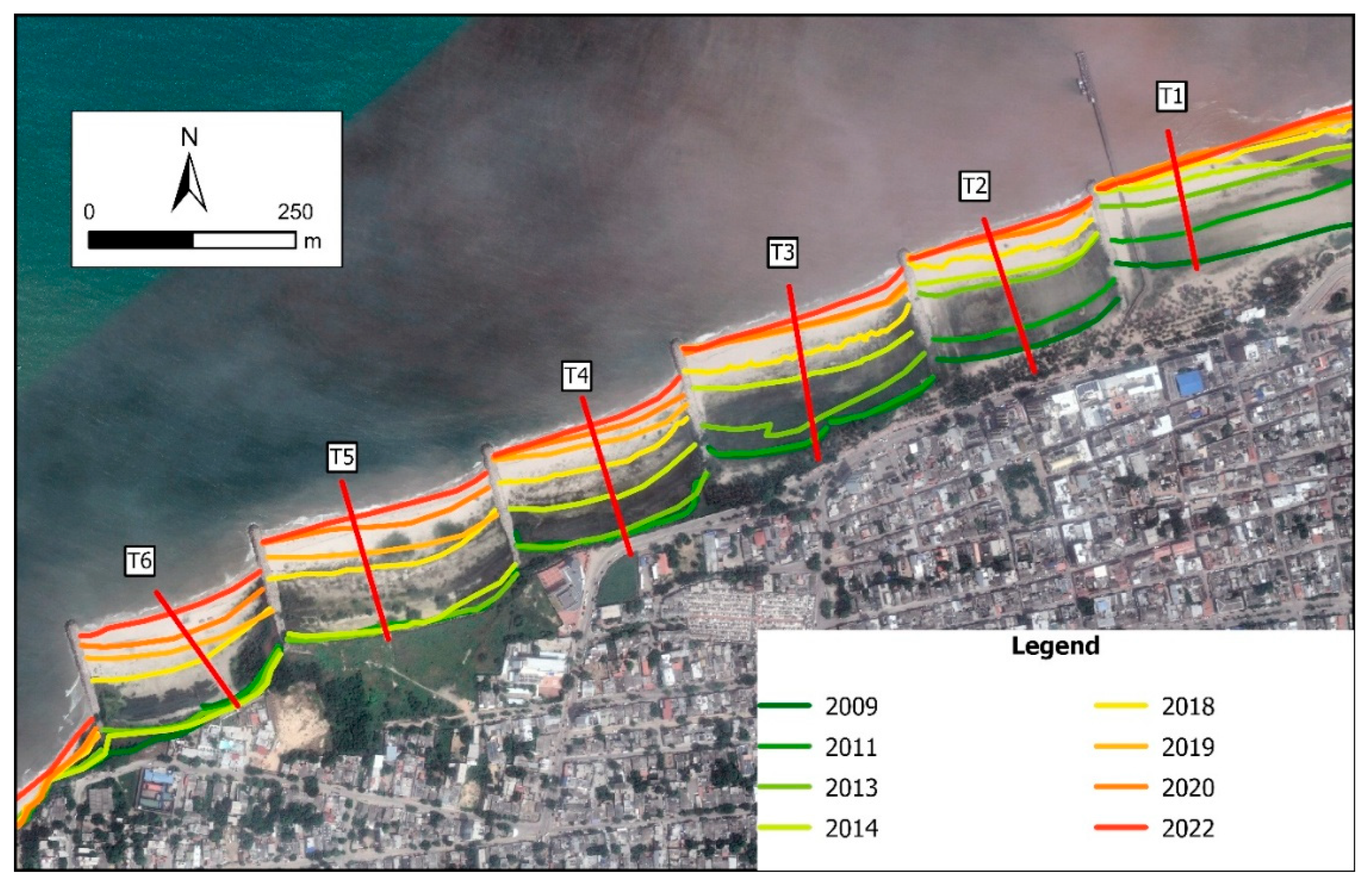
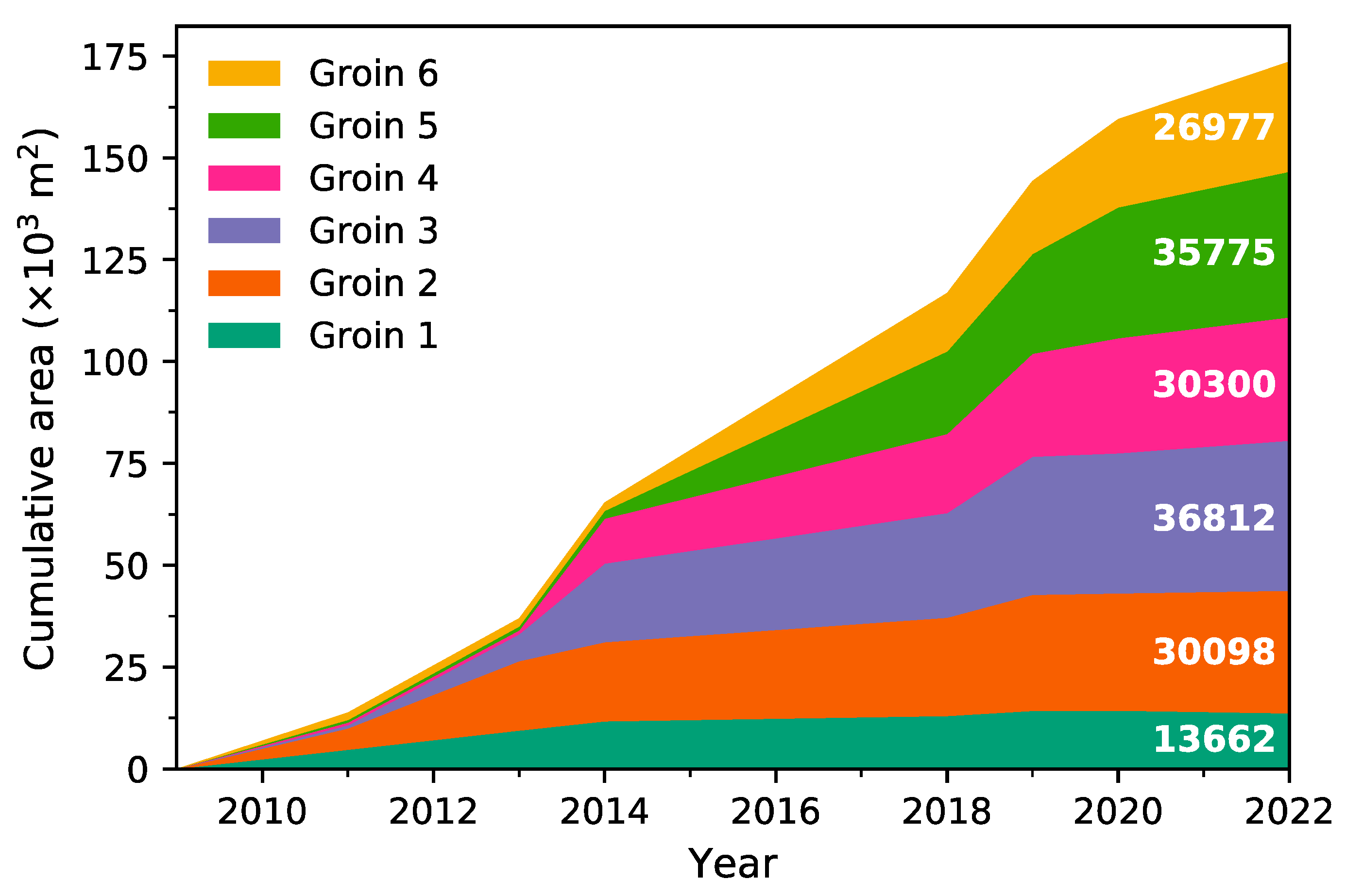
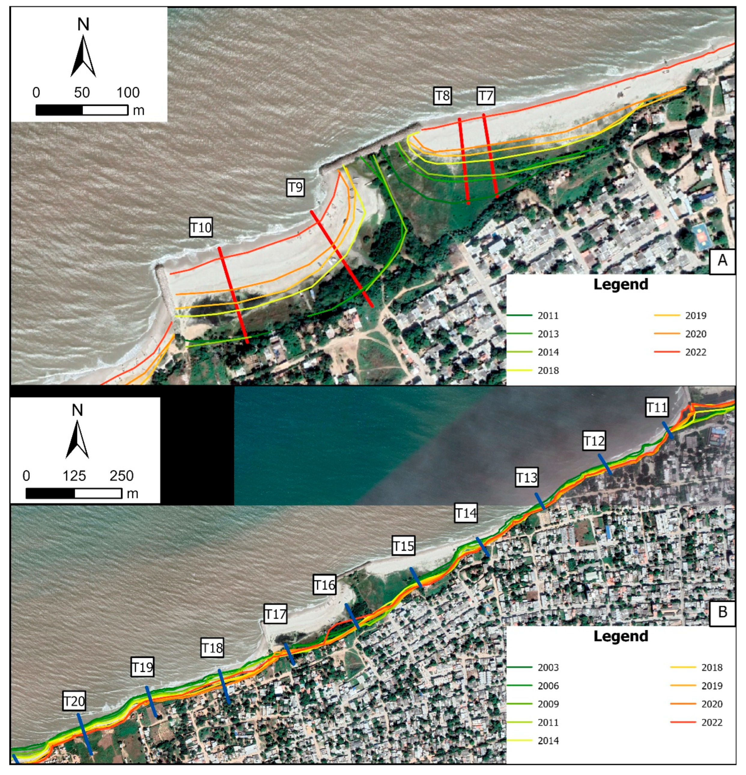
4.1. Zone 1: Effect of the Groins

Table 2. Displacement rates of the coastline for the different transects created in Zone 1.

Period	Transect	NSM (m)	LRR (m/yr)	LCI (m/yr)	LR2
1987–2006	T1	−2.1	−0.3	4.4	0.43
	T2	−3.3	−0.4	3.3	0.72
	T3	−4.9	−0.5	0.7	0.99
	T4	−4.3	−0.5	2.7	0.85
	T5	−7.2	−0.8	3.8	0.89
	T6	−4.0	−0.5	5.7	0.58
2009–2022	T1	81.1	6.5	3.7	0.80
	T2	118.6	9.3	3.9	0.88
	T3	146.6	13.2	3.6	0.95
	T4	138.0	13.1	2.5	0.97
	T5	134.9	13.6	4.9	0.91
	T6	129.5	12.3	4.4	0.91

shows the results of the analysis of shorelines with the DSAS program in Zone 1. This analysis has been divided into two time periods: 1987–2006 (before the construction of the groins) and 2009–2022 (after). For the 1987–2006 period, only three images are available, with the 1987 image serving as the baseline. Therefore, the regression data should be interpreted with caution. Nonetheless, it is evident that the coastal dynamics were predominantly erosive, with an average shoreline change of 5.3 ± 1.2 m between 1987 and 2006. For the 2009–2022 period, the availability of more images allows for more reliable fitting results, better capturing the variability in shoreline dynamics. During this period, the construction of the groins led to a high mean accretion rate of 11.3 ± 2.8 m/yr across the six analyzed transects. The sediment retention effect caused by the construction of the groins on littoral dynamics is clear (see shoreline evolution in Figure 4). From 2009 to 2013, significant beach growth was observed upstream of groins 1, 2, and 3 (Figure 5). Between 2014 and 2018, this growth was even more pronounced across all transects, leading to the almost complete silting up of groins 1 and 2. A similar trend is observed between 2018 (see Figure 2) and 2020, with notable beach advance between groins 3 and 6. Since 2020, the growth has slowed in nearly all groins, except for groins 5 and 6, which are the last to become silted (Figure 5). The further west, the later the gaps between groins are filled, all within a time interval of about 5 years. It is likely that, soon, sand will bypass these groins and advance again towards the areas located southwest, as has been observed in other coastal locations [65].

A one-way analysis of variance (ANOVA) was conducted to evaluate whether there were statistically significant differences in NSM between the two time intervals (see

Table 3. ANOVA for the NSM.

Source	Sum of Squares	Degrees of Freedom	Mean Sum of Squares	F	p-Value
Period	49,987.5	1	49,987.5	182.68	9.47 × 10−8
Error	2736.4	10	273.6
Total	52,723.9	11

). The mean NSM for the 1987–2006 period was substantially lower (p-value < 0.001) compared to the 2009–2022 period. These findings suggest a statistically significant shift in shoreline dynamics over time, indicating a notable change in coastal behavior.

It is not appropriate to apply prediction models based on the historical shoreline evolution of recent years in this case. This is because the coastal dynamics are likely to change once the shoreline reaches the end of the groins, altering the physical conditions. If the models were to follow the trend of the last decade, they would predict an unrealistic extension of beach accretion hundreds of meters beyond the groins. Additionally, it is not meaningful to use the models to predict when the space between the groins will be filled. The rates (LRR) calculated in the previous years are quite high compared to the remaining distances in each groin. For example, recent field measurements (February 2024) show that groin 1 is already filled. Similar situations occur with the other groins, where the distance between the shoreline and the end of the groins was as follows: 2024: 5 m for groin 2; 7.8 m for groin 3; 5.8 m for groin 4; 6.9 m for groin 5; and 6.4 m for groin 6.

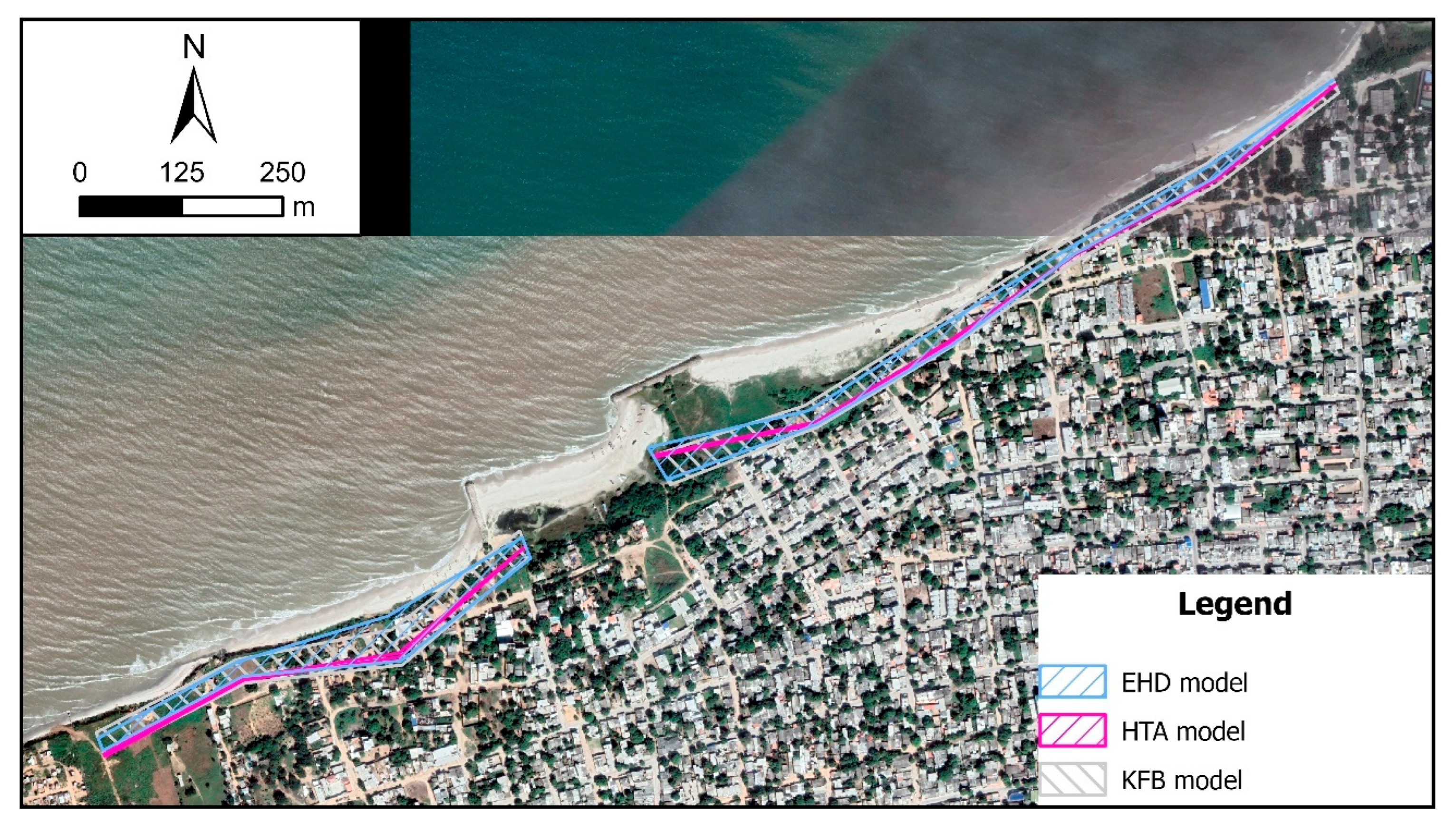
4.2. Zone 2: Urban Cliff Area with Seawall

Since the construction of coastal structures, sediment accumulation in this area has been remarkable (see NSM in

Table 4. Displacement rates of the coastline for the different transects created during the period 2009–2022 for the beach area in Zone 2.

Transect	NSM (m)	LRR (m/yr)	LCI (m/yr)	LR2
T7	67.7	6.2	2.9	0.90
T8	65.1	5.9	2.7	0.90
T9	87.6	8.6	2.3	0.98
T10	90.9	10.0	4.7	0.94

). In all profiles, the coefficients of determination indicate that the linear model used is reliable. However, once again, applying prediction models in this area is not appropriate, as the sediment retention zone of these structures is nearly filled (Figure 6A). The southern part of the seawall has experienced particularly significant growth, with an average gain of approximately 89 m over just 13 years (2009–2022), most of which has occurred since 2018 (yellow line in Figure 6A).

Table 5. Displacement rates of the coastline extracted from the DSAS for the cliff in Zone 2 and results of the prediction models. * Means low LR2 values and therefore the fit is not reliable.

Transect	DSAS Years 2003–2022				HTA		EHD		KFB
	NSM (m)	LRR (m/yr)	LCI (m/yr)	LR2	Lower Bound	Upper Bound	Lower Bound	Upper Bound	Lower Bound	Upper Bound
T11	−1.5	−0.1	0.2	0.26 *	N/A	N/A	N/A	N/A	N/A	N/A
T12	−11.6	−0.9	0.4	0.86	−28.4	−30.8	−11.5	−27.6	−7.6	−37.0
T13	−8.7	−0.5	0.2	0.85	−16.0	−17.4	−6.2	−15.9	2.6	−24.3
T14	−15.6	−0.7	0.6	0.61	−24.1	−26.1	−3.5	−29.7	2.2	−31.4
T15	−13.0	−0.7	0.4	0.70	−21.8	−23.6	−5.1	−24.8	2.6	−28.4
T16	21.8	0.9	1.0	0.44 *	N/A	N/A	N/A	N/A	N/A	N/A
T17	−4.2	0.2	0.6	0.10 *	N/A	N/A	N/A	N/A	N/A	N/A
T18	−17.1	−1.8	1.3	0.67	−59.6	−64.5	−12.2	−69.7	−29.7	−74.9
T19	−15.5	−1.1	0.4	0.87	−36.5	−39.5	−15.4	−34.7	−12.7	−43.6
T20	−18.8	−1.2	0.4	0.92	−40.5	−43.9	−19.6	−36.1	−12.4	−42.1

summarizes the DSAS data for cliff Zone 2 (Figure 6), where most transects (T12–T20, except T16 and T17) show significant erosion, particularly T18. Indeed, in recent years, there have been several instances of houses collapsing or facing imminent collapse north of the seawall. The reliability of the linear fit is high for these transects, but low LR2 values in T11, T16, and T17 indicate poor model fit. T11, located downstream of groin No. 6, is influenced by its construction [66], while T16 and T17 have a developing beach and vegetation growth, complicating cliff crest identification. Due to these factors, prediction models were not applied to these transects.

The HTA and EHD models simulate shoreline changes from the last available coastline (2022) to 2045, while the KFB model in DSAS estimates 20 years from 2024, rounding up to provide predictions for 2045. All three models project significant shoreline recession, particularly south of the seawall in T18, T19, and T20 (Figure 7), with lower erosion estimates in the northern part. In the KFB model, accretion estimates for the lower bound at T13, T14, and T15 stem from data uncertainty rather than a physical process. The HTA model shows the smallest prediction variability, while the KFB model has the largest range. In most transects, the three models overlap or closely align (Figure 7), making this common range the most reliable forecast for territorial planning.

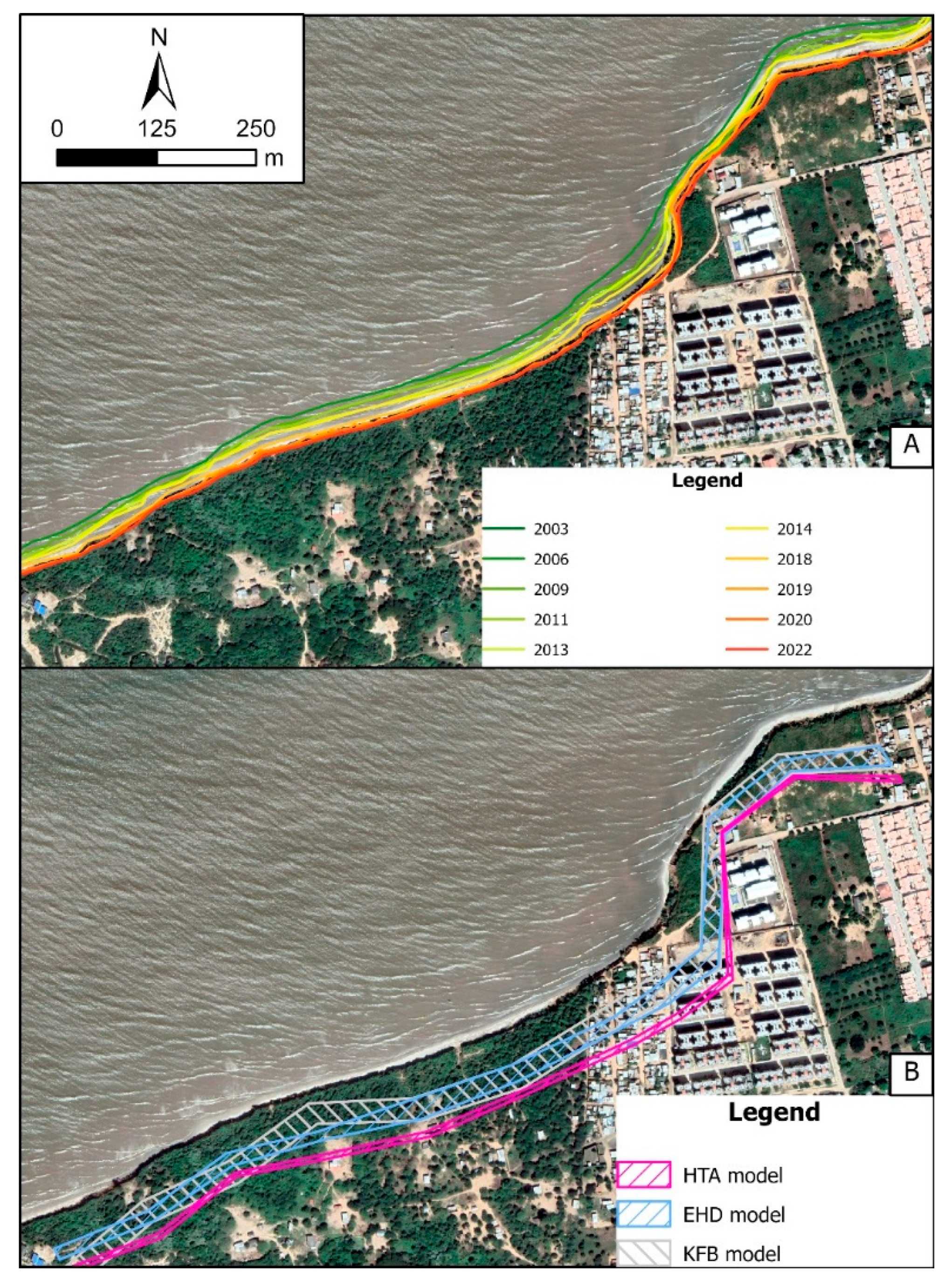
4.3. Zone 3: Cliff Area

Table 6. Displacement rates of the coastline extracted from DSAS in Zone 3 and results of the prediction models.

Transect	DSAS Years 2003–2022				HTA		EHD		KFB
	NSM (m)	LRR (m/yr)	LCI (m/yr)	LR2	Lower Bound	Upper Bound	Lower Bound	Upper Bound	Lower Bound	Upper Bound
T21	−45.8	−2.9	0.6	0.94	−97.7	−105.9	−52.9	−81.4	−51.3	−86.0
T22	−27.9	−1.5	0.4	0.91	−49.2	−53.3	−25.1	−42.6	−16.1	−46.2
T23	−18.9	−0.8	0.6	0.51	−26.4	−28.6	−3.7	−32.7	3.9	−31.0
T24	−49.4	−3.1	0.7	0.94	−103.0	−111.7	−55.7	−86.0	−54.4	−89.8
T25	−45.9	−2.9	0.6	0.94	−96.0	−104.0	−52.7	−79.4	−50.1	−84.1
T26	−41.5	−2.6	0.4	0.97	−87.7	−95.0	−51.8	−68.8	−44.0	−73.9
T27	−38.4	−2.3	0.5	0.94	−76.3	−82.7	−41.6	−63.3	−36.6	−68.5
T28	−38.5	−2.5	0.4	0.96	−84.3	−91.4	−48.8	−67.2	−43.0	−73.4
T29	−37.7	−2.3	0.3	0.98	−78.0	−84.4	−47.6	−59.6	−38.3	−66.1
T30	−27.8	−1.7	0.4	0.93	−58.2	−63.1	−31.3	−48.8	−23.7	−53.8
T31	−37.3	−2.3	0.3	0.97	−76.3	−82.7	−45.1	−59.8	−36.2	−65.1
T32	−34.3	−2.1	0.3	0.96	−68.6	−74.3	−39.6	−54.7	−32.3	−61.4

shows a mean NSM of −37 m in Zone 3, with an average LRR of −2.3 m/yr, indicating significant cliff-top recession. The LRR variability is moderate (mean LCI: 0.66 m/yr), and the confidence in these estimates (LR2) averages 0.9 across all transects. Transects T22 and T23 exhibit lower erosion due to the cliff’s orientation against predominant waves and currents from the west (Figure 8A). Unlike Zone 2, the cliffs in Zone 3 increase in height westward, making them more geotechnically unstable and likely contributing to higher recession rates. However, recent data (Figure 8A) suggest a slowdown in retreat. The absence of a protective beach intensifies erosion [67], likely due to sediment retention by groins in Zone 1. The lack of pre-2003 images for Zone 3 complicates assessing the groins’ impact on their natural dynamics.

Between 2014 and 2018, urban development advanced into this area despite evident cliff recession (Figure 9). By 2021, urbanization peaked, but in 2022, some buildings near the cliff were removed (red box in Figure 9). This city expansion highlights the absence of a coastal geomorphodynamics study like this one. The three prediction models estimate a significant recession by 2045 (Figure 8B, Table 5). At T23, the lower bound of the KFB model suggests cliff accretion, which is unrealistic without human intervention and should be disregarded. The HTA model predicts the highest recession rates but with lower variability, while the EHD and KFB models provide similar estimates, though the latter shows greater dispersion. The EHD model’s prediction band falls within the KFB model’s range, reinforcing their consistency (Figure 8B). Agreement between models enhances confidence in predictions, narrowing probable outcomes and improving risk assessments for land management [68]. By 2045, cliff retreat is projected to impact buildings at T21, T24, T25, and T26, highlighting the need for the Municipality of Riohacha to integrate these findings into land-use planning, particularly considering the overlapping EHD-KFB model area.

Table 7. Variation of the area eroded in Zone 3.

Period	Years	Area Change (m2)	Rate of Area Change (m2/yr)
2003–2006	3	−7058	−2353
2006–2009	3	−13,115	−4372
2009–2011	2	−5635	−2817
2011–2013	2	−1733	−867
2013–2014	1	−5239	−5239
2014–2018	4	−13,446	−3361
2018–2019	1	−7758	−7785
2019–2020	1	−1356	−1356
2020–2022	2	−2715	−1358

presents the rate of change in eroded material in Zone 3, showing fluctuations over different periods based on available imagery. Annual surface loss varies significantly, with extreme erosion events primarily linked to severe marine conditions caused by hurricanes and cold fronts, often associated with El Niño Southern Oscillation (ENSO) [1,15]. Between 2003 and 2022, Colombia’s Caribbean region experienced variable storm activity, with particularly active periods in 2005–2010, 2013, and 2016–2019, aligning with the most intense erosion phases. These peaks in hurricane activity were often driven by La Niña or ENSO-neutral conditions. In addition to storm activity, the erosion in Zone 3 may also be influenced by sediment retention caused by the groins built between 2006 and 2009. This period coincides with a phase of intense erosion in Zone 3, suggesting a possible connection. From 2009 to 2018, sediment retention was substantial (see Figure 5), aligning with the highest cliff recession rates in this area. However, since 2019–2020, with most groins nearly filled, erosion appears to have slowed (last column in Table 7). This trend suggests that once sediment retention reaches capacity, some equilibrium may be reestablished, potentially reducing erosion rates. As has been shown in other work [53], while groins promote sand accumulation, they can also induce significant alterations in adjacent areas, particularly downstream of their location. The possible link between groin-induced sediment trapping and increased erosion in Zone 3 requires further investigation to better understand the long-term coastal dynamics and improve future shoreline management strategies. It should also be noted that the intensification of extreme climate events under climate change could potentially enhance the influence of ENSO on coastal erosion processes in this region. ENSO phases are known to modulate storm frequency, wave energy, and precipitation patterns in the Caribbean, leading to variations in sediment transport and shoreline stability [1]. For instance, El Niño conditions often reduce tropical cyclone activity but can intensify dry seasons, potentially lowering sediment supply from riverine inputs, while La Niña tends to promote more frequent and intense storms that can accelerate coastal erosion. In the context of Riohacha, such shifts could exacerbate localized erosion hotspots, particularly near infrastructure-like groins, by altering nearshore currents and sediment dynamics. However, quantifying these impacts remains challenging due to the lack of high-resolution temporal and spatial data linking ENSO indices with coastal morphological changes in the study area. Future studies should integrate regional climate data, hydrodynamic modeling, and long-term shoreline monitoring to better understand and predict the compounded effects of ENSO variability and climate change on shoreline evolution.

5. Conclusions

This study analyzes the coastal evolution of the urban area of Riohacha, capital of the Department of La Guajira, Colombia, between 1987 and 2022. To assess the vulnerability of this shoreline over the next 20 years, historical coastline changes—both in beach and cliff zones—were analyzed using aerial and satellite imagery alongside GIS tools.

The construction of a series of groins near the mouth of the Ranchería River has profoundly altered coastal dynamics, promoting sediment accumulation within the groin field while intensifying erosion in downstream cliff areas. The findings indicate a shift from an erosional to an accretional regime in the groin-affected zone, where the spaces between the 150 m long structures became completely silted in just a decade. However, this sediment retention has likely disrupted the natural sediment supply to adjacent areas, accelerating cliff erosion downstream and increasing the risk to nearby buildings.

To estimate the extent of future coastal changes, three predictive models (incorporating uncertainty assessments) were applied: Historical Trend Analysis (HTA), Extrapolation from Historical Data (EHD), and a Kalman filter-based (KFB) model. The overlap between the uncertainty bands of different models identifies the most probable locations of the future cliff crest by 2045. In the most severe scenario, if current conditions do not change, coastal retreat could reach 86 m, which would greatly affect the local community.

The methodology and findings presented in this study are crucial for optimizing short- and medium-term coastal management strategies, particularly in areas with significant anthropogenic interventions. These results provide essential insights for assessing potential social, environmental, and economic losses, guiding land-use planning, and informing the design of mitigation measures to address ongoing and future erosion hazards.

References

1. Vallarino Castillo, R.; Negro Valdecantos, V.; del Campo, J.M. Understanding the Impact of Hydrodynamics on Coastal Erosion in Latin America: A Systematic Review. Front. Environ. Sci. 2023, 11, 1267402. [Google Scholar] [CrossRef]
2. Velsamy, S.; Balasubramaniyan, G.; Swaminathan, B.; Kesavan, D. Multi-Decadal Shoreline Change Analysis in Coast of Thiruchendur Taluk, Thoothukudi District, Tamil Nadu, India, Using Remote Sensing and DSAS Techniques. Arab. J. Geosci. 2020, 13, 838. [Google Scholar] [CrossRef]
3. Pagán, J.I.; Aragonés, L.; Tenza-Abril, A.J.; Pallarés, P. The Influence of Anthropic Actions on the Evolution of an Urban Beach: Case Study of Marineta Cassiana Beach, Spain. Sci. Total Environ. 2016, 559, 242–255. [Google Scholar] [CrossRef] [PubMed]
4. Unguendoli, S.; Biolchi, L.G.; Aguzzi, M.; Pillai, U.P.A.; Alessandri, J.; Valentini, A. A Modeling Application of Integrated Nature Based Solutions (NBS) for Coastal Erosion and Flooding Mitigation in the Emilia-Romagna Coastline (Northeast Italy). Sci. Total Environ. 2023, 867, 161357. [Google Scholar] [CrossRef] [PubMed]
5. Alves, B.; Angnuureng, D.B.; Morand, P.; Almar, R. A Review on Coastal Erosion and Flooding Risks and Best Management Practices in West Africa: What Has Been Done and Should Be Done. J. Coast. Conserv. 2020, 24, 38. [Google Scholar] [CrossRef]
6. Arabadzhyan, A.; Figini, P.; García, C.; González, M.M.; Lam-González, Y.E.; León, C.J. Climate Change, Coastal Tourism, and Impact Chains–a Literature Review. Curr. Issues Tour. 2021, 24, 2233–2268. [Google Scholar] [CrossRef]
7. Natarajan, L.; Sivagnanam, N.; Usha, T.; Chokkalingam, L.; Sundar, S.; Gowrappan, M.; Roy, P.D. Shoreline Changes over Last Five Decades and Predictions for 2030 and 2040: A Case Study from Cuddalore, Southeast Coast of India. Earth Sci. Inform. 2021, 14, 1315–1325. [Google Scholar] [CrossRef]
8. Ayyam, V.; Palanivel, S.; Chandrakasan, S. Coastal Ecosystems of the Tropics-Adaptive Management; Springer: Singapore, 2019. [Google Scholar]
9. Calil, J.; Reguero, B.G.; Zamora, A.R.; Losada, I.J.; Méndez, F.J. Comparative Coastal Risk Index (CCRI): A Multidisciplinary Risk Index for Latin America and the Caribbean. PLoS ONE 2017, 12, e0187011. [Google Scholar] [CrossRef] [PubMed]
10. Wang, Y.; Jiménez, C.; Moreno, N.; Wang, P. Tsunami Characteristics and Source Estimation of the 2024 Yauca (Peru) Earthquake. Ocean. Eng. 2025, 331, 121325. [Google Scholar] [CrossRef]
11. Silva, R.; Martínez, M.L.; Hesp, P.A.; Catalan, P.; Osorio, A.F.; Martell, R.; Fossati, M.; Da Silva, G.M.; Mariño-Tapia, I.; Pereira, P.; et al. Present and Future Challenges of Coastal Erosion in Latin America. J. Coast. Res. 2014, 11, 1–16. [Google Scholar] [CrossRef]
12. Rangel-Buitrago, N.; Gracia, C.A. From the Closet to the Shore: Fashion Waste Pollution on Colombian Central Caribbean Beaches. Mar. Pollut. Bull. 2024, 199, 115976. [Google Scholar] [CrossRef] [PubMed]
13. Salazar, F.J.; Ramirez, H.M. Evaluation of Coastal Erosion in the Jurisdiction of the Municipalities of Puerto Colombia and Tubara, Atlantico, Colombia in Google Earth Engine with Landsat and Sentinel 2 Images. Int. J. Geol. Environ. Eng. 2023, 17, 128–146. [Google Scholar]
14. Botero, C.; Anfuso, G.; Rangel-Buitrago, N.; Correa, I.D. Coastal Erosion Monitoring in Colombia: Overview and Study Cases on Caribbean and Pacific Coasts; Universidad de Cádiz: Cádiz, Spain, 2013. [Google Scholar]
15. Martínez-Pérez, E.J.; Arévalo-Quintero, J.S. Estudio y Plan de Control de La Erosión Costera Mediante Estructuras de Protección Costera En Una Playa de La Ciudad de Riohacha, La Guajira; Universidad Católica De Colombia: Bogota, Colombia, 2022. [Google Scholar]
16. Rangel-Buitrago, N.G.; Anfuso, G.; Williams, A.T. Coastal Erosion along the Caribbean Coast of Colombia: Magnitudes, Causes and Management. Ocean. Coast. Manag. 2015, 114, 129–144. [Google Scholar] [CrossRef]
17. Alvarez-Cuesta, M.; Toimil, A.; Losada, I.J. Modelling Long-Term Shoreline Evolution in Highly Anthropized Coastal Areas. Part 1: Model Description and Validation. Coast. Eng. 2021, 169, 103960. [Google Scholar] [CrossRef]
18. Apostolopoulos, D.; Nikolakopoulos, K. A Review and Meta-Analysis of Remote Sensing Data, GIS Methods, Materials and Indices Used for Monitoring the Coastline Evolution over the Last Twenty Years. Eur. J. Remote Sens. 2021, 54, 240–265. [Google Scholar] [CrossRef]
19. Crowell, M.; Leatherman, S.P.; Buckley, M.K. Shoreline Change Rate Analysis: Long Term Versus Short Term Data. Shore Beach 1993, 61, 13–20. [Google Scholar]
20. Castedo, R.; de la Vega-Panizo, R.; Fernández-Hernández, M.; Paredes, C. Measurement of Historical Cliff-Top Changes and Estimation of Future Trends Using GIS Data between Bridlington and Hornsea–Holderness Coast (UK). Geomorphology 2015, 230, 146–160. [Google Scholar] [CrossRef]
21. Ponte Lira, C.; Taborda, R.; Silva, A.N.; Andrade, C. Challenges and New Strategies in Assessing Multidecadal Shore Platform Sandy Beach Evolution from Aerial Imagery. Mar. Geol. 2021, 436, 106472. [Google Scholar] [CrossRef]
22. Leisner, M.M.; de Paula, D.P.; Alves, D.C.L.; da Guia Albuquerque, M.; de Holanda Bastos, F.; Vasconcelos, Y.G. Long-Term and Short-Term Analysis of Shoreline Change and Cliff Retreat on Brazilian Equatorial Coast. Earth Surf. Process Landf. 2023, 48, 2987–3002. [Google Scholar] [CrossRef]
23. Yadav, A.; Kuntoji, G.; Hiremath, C.G.; Narasimha, N.H.; Mutagi, S. Automatic Detection and Analysis of the Shoreline Change Rate at Maravanthe Coast, India. Mar. Geod. 2024, 47, 395–414. [Google Scholar] [CrossRef]
24. Morales, J.A. Human Impacts on Coastal Systems; Springer: Cham, Switzerland, 2022; pp. 423–435. [Google Scholar]
25. Villamizar, A.; Gutiérrez, M.E.; Nagy, G.J.; Caffera, R.M.; Leal Filho, W. Climate Adaptation in South America with Emphasis in Coastal Areas: The State-of-the-Art and Case Studies from Venezuela and Uruguay. Clim. Dev. 2017, 9, 364–382. [Google Scholar] [CrossRef]
26. Winckler, P.; Martín, R.A.; Esparza, C.; Melo, O.; Sactic, M.I.; Martínez, C. Projections of Beach Erosion and Associated Costs in Chile. Sustainability 2023, 15, 5883. [Google Scholar] [CrossRef]
27. Islam, M.S.; Crawford, T.W. Assessment of Spatio-Temporal Empirical Forecasting Performance of Future Shoreline Positions. Remote Sens. 2022, 14, 6364. [Google Scholar] [CrossRef]
28. Palanisamy, P.; Sivakumar, V.; Velusamy, P.; Natarajan, L. Spatio-Temporal Analysis of Shoreline Changes and Future Forecast Using Remote Sensing, GIS and Kalman Filter Model: A Case Study of Rio de Janeiro, Brazil. J. S. Am. Earth Sci. 2024, 133, 104701. [Google Scholar] [CrossRef]
29. Ülger, M.; Tanrıvermiş, Y. Prevention of the Effects of Coastal Structures on Shoreline Change Using Numerical Modeling. Ocean. Coast. Manag. 2023, 243, 106752. [Google Scholar] [CrossRef]
30. Yu, H.; Weng, Z.; Chen, G.; Chen, X. Improved XBeach Model and Its Application in Coastal Beach Evolution under Wave Action. Coast. Eng. J. 2023, 65, 560–571. [Google Scholar] [CrossRef]
31. Ciccaglione, M.C.; Buccino, M.; Calabrese, M. On the Evolution of Beaches of Finite Length. Cont. Shelf. Res. 2023, 259, 104990. [Google Scholar] [CrossRef]
32. Stronkhorst, J.; Levering, A.; Hendriksen, G.; Rangel-Buitrago, N.; Appelquist, L.R. Regional Coastal Erosion Assessment Based on Global Open Access Data: A Case Study for Colombia. J. Coast. Conserv. 2018, 22, 787–798. [Google Scholar] [CrossRef]
33. Martínez, J.; Yokoyama, Y.; Gomez, A.; Delgado, A.; Matsuzaki, H.; Rendon, E. Late Holocene Marine Terraces of the Cartagena Region, Southern Caribbean: The Product of Neotectonism or a Former High Stand in Sea-Level? J. S. Am. Earth Sci. 2010, 29, 214–224. [Google Scholar] [CrossRef]
34. Rangel-Buitrago, N.; Williams, A.T.; Anfuso, G. Hard Protection Structures as a Principal Coastal Erosion Management Strategy along the Caribbean Coast of Colombia. A Chronicle of Pitfalls. Ocean. Coast. Manag. 2018, 156, 58–75. [Google Scholar] [CrossRef]
35. IDEAM Boletín Condiciones Hidrometeorológicas. Available online: https://www.ideam.gov.co/sala-de-prensa/boletines (accessed on 14 February 2024).
36. Andrade, C.A. Cambios Recientes Del Nivel Del Mar En Colombia. Deltas de Colombia: Morfodinámica y Vulnerabilidad Ante El Cambio Global; Fondo Editorial Universidad EAFIT: Medellín, Colombia, 2008; pp. 101–121. [Google Scholar]
37. Corpoguajira. Invemar Atlas Marino Costero de La Guajira; Corpoguajira: Riohacha, Colombia, 2012; ISBN 9789588448459.
38. Restrepo, J.C.; Otero, L.; Casas, A.C.; Henao, A.; Gutiérrez, J. Shoreline Changes between 1954 and 2007 in the Marine Protected Area of the Rosario Island Archipelago (Caribbean of Colombia). Ocean. Coast. Manag. 2012, 69, 133–142. [Google Scholar] [CrossRef]
39. Restrepo, J.D.; López, S.A. Morphodynamics of the Pacific and Caribbean Deltas of Colombia, South America. J. S. Am. Earth Sci. 2008, 25, 1–21. [Google Scholar] [CrossRef]
40. Restrepo-Ángel, J.D.; Mora-Páez, H.; Díaz, F.; Govorcin, M.; Wdowinski, S.; Giraldo-Londoño, L.; Tosic, M.; Fernández, I.; Paniagua-Arroyave, J.F.; Duque-Trujillo, J.F. Coastal Subsidence Increases Vulnerability to Sea Level Rise over Twenty First Century in Cartagena, Caribbean Colombia. Sci. Rep. 2021, 11, 18873. [Google Scholar] [CrossRef] [PubMed]
41. Berrio, Y.; Rivillas-Ospina, G.; Ruiz-Martínez, G.; Arango-Manrique, A.; Ricaurte, C.; Mendoza, E.; Silva, R.; Casas, D.; Bolívar, M.; Díaz, K. Energy Conversion and Beach Protection: Numerical Assessment of a Dual-Purpose WEC Farm. Renew. Energy 2023, 219, 119555. [Google Scholar] [CrossRef]
42. Rangel-Buitrago, N.; Melfi, G.A. Morfología, Morfodinámica y Evolución Reciente En La Península de La Guajira, Caribe Colombiano. Rev. Cienc. Ing. Día 2013, 8, 2357–5409. [Google Scholar]
43. Ballén, S.; Barrios, J.D. Cuantificación de Las Transformaciones Territoriales Asociadas a Dinámicas de Producción Derivadas de Los Diferentes Sectores Productivos En La Cuenca Del Río Ranchería, La Guajira, Colombia; Universidad Santo Tomás: Antioquia, Colombia, 2019. [Google Scholar]
44. Rodríguez, G.; Londoño, A.C. Mapa Geológico Del Departamento de La Guajira; Ministerio de Minas y Energía: Bogotá, Colombia, 2002.
45. Mosquera, F.; Arango, J.; Carreño, J.; Aguilera, H. Exploración de Acuíferos de La Alta y Media Guajira. Capítulo I, Geología; Instituto Nacional de Investigaciones Geológico Mineras: Bogotá, Colombia, 1976. [Google Scholar]
46. Granados, A. Resumen Del Estudio Hidrogeológico de La Media y Baja Guajira. Boletín Geológico 1988, 29, 45–83. [Google Scholar] [CrossRef]
47. Molina, L.; Pérez, F.; Martínez, J.; Franco, V.; Marín, L.; González, J.; Carvajal, J. Geomorfología y Aspectos Erosivos Del Litoral Caribe Colombiano. INGEOMINAS 1998, 21, 1–73. [Google Scholar]
48. Himmelstoss, E.A.; Henderson, R.E.; Kratzmann, M.G.; Farris, A.S. Shoreline Analysis System (DSAS). User Guide; U.S. Geological Survey: Reston, VA, USA, 2021; pp. 1–104.
49. IGAC Web Page of the Instituto Geográfico Agustín Codazzi. Available online: https://www.igac.gov.co/ (accessed on 3 February 2024).
50. Google Earth Pro Google Earth Pro. Available online: https://www.google.es/intl/es/earth/index.html (accessed on 9 January 2024).
51. AgiSoft AgiSoft PhotoScan Professional. Available online: http://www.agisoft.com/downloads/installer/ (accessed on 2 February 2023).
52. Tsiakos, C.A.D.; Chalkias, C. Use of Machine Learning and Remote Sensing Techniques for Shoreline Monitoring: A Review of Recent Literature. Appl. Sci. 2023, 13, 3268. [Google Scholar] [CrossRef]
53. Ojeda Zújar, J.P.; Fernández Núñez, M.; Prieto Campos, A.; Pérez Alcántara, J.P.; Vallejo Villalta, I. Levantamiento de Líneas de Costa a Escalas de Detalle Para El Litoral de Andalucía: Criterios, Modelo de Datos y Explotación. In Proceedings of the Congreso Nacional de Tecnologías de la Información Geográfica, Sevilla, Spain, 13–17 September 2010; pp. 324–336. [Google Scholar]
54. Fernández-Hernández, M.; Calvo, A.; Iglesias, L.; Castedo, R.; Ortega, J.J.; Diaz-Honrubia, A.J.; Mora, P.; Costamagna, E. Anthropic Action on Historical Shoreline Changes and Future Estimates Using GIS: Guardarmar Del Segura (Spain). Appl. Sci. 2023, 13, 9792. [Google Scholar] [CrossRef]
55. Nithu Raj, R.; Rejin Nishkalank, A.; Chrisben Sam, S. Coastal Shoreline Changes in Chennai: Environment Impacts and Control Strategies of Southeast Coast. In Handbook of Environmental Materials Management; Springer: Cham, Switzerland, 2020; pp. 1–14. [Google Scholar]
56. Environmental Systems Research Institute ESRI—Environmental Systems Research Institute 2024. Available online: https://www.esri.com/en-us/home (accessed on 9 January 2024).
57. Davidson, M.A.; Lewis, R.P.; Turner, I.L. Forecasting Seasonal to Multi-Year Shoreline Change. Coast. Eng. 2010, 57, 620–629. [Google Scholar] [CrossRef]
58. Hunt, E.; Davidson, M.; Steele, E.C.C.; Amies, J.D.; Scott, T.; Russell, P. Shoreline Modelling on Timescales of Days to Decades. In Cambridge Prisms: Coastal Futures; Cambridge University Press: Cambridge, UK, 2023; Volume 1. [Google Scholar] [CrossRef]
59. Ciritci, D.; Türk, T. Assessment of the Kalman Filter-Based Future Shoreline Prediction Method. Int. J. Environ. Sci. Technol. 2020, 17, 3801–3816. [Google Scholar] [CrossRef]
60. Leatherman, S.P. Modelling Shore Response to Sea-Level Rise on Sedimentary Coasts. Prog. Phys. Geogr. 1990, 14, 447–464. [Google Scholar] [CrossRef]
61. Lee, E.M.; Clark, A.R. Investigation and Management of Soft Rock Cliffs; Thomas Telford: London, UK, 2002. [Google Scholar]
62. Mishra, M.; Chand, P.; Beja, S.K.; Santos, C.A.G.; da Silva, R.M.; Ahmed, I.; Kamal, A.H.M. Quantitative Assessment of Present and the Future Potential Threat of Coastal Erosion along the Odisha Coast Using Geospatial Tools and Statistical Techniques. Sci. Total Environ. 2023, 875, 162488. [Google Scholar] [CrossRef] [PubMed]
63. Kalman, R.E. A New Approach to Linear Filtering and Prediction Problems. J. Basic Eng. 1960, 82, 35–45. [Google Scholar] [CrossRef]
64. Long, J.W.; Plant, N.G. Extended Kalman Filter Framework for Forecasting Shoreline Evolution. Geophys. Res. Lett. 2012, 39, 1–6. [Google Scholar] [CrossRef]
65. Griggs, G.; Patsch, K.; Lester, C.; Anderson, R. Groins, Sand Retention, and the Future of Southern California’s Beaches. Shore Beach 2020, 88, 14–36. [Google Scholar] [CrossRef] [PubMed]
66. U.S. Army Corps of Engineers. Corps of Engineers Coastal Groins and Nearshore Breakwaters Engineer Manual; Department of the Army, U.S. Army Corps of Engineers: Washington, DC, USA, 1992.
67. Castedo, R.; Fernández, M.; Trenhaile, A.S.; Paredes, C. Modeling Cyclic Recession of Cohesive Clay Coasts: Effects of Wave Erosion and Bluff Stability. Mar. Geol. 2013, 335, 162–176. [Google Scholar] [CrossRef]
68. Tierolf, L.; Haer, T.; Athanasiou, P.; Luijendijk, A.P.; Botzen, W.J.W.; Aerts, J.C.J.H. Coastal Adaptation and Migration Dynamics under Future Shoreline Changes. Sci. Total Environ. 2024, 917, 170239. [Google Scholar] [CrossRef] [PubMed]
Figure 1. Location of the study area and division into three work zones. Satellite image taken from Google Earth Pro, corresponding to the year 2024.
Applsci 15 08119 g001
Figure 2. Aerial image year 2018. Source: Google Earth Pro. (A) Zone 1 of the study area with the 6 groins numbered from north to south. (B) Zone 2 with the seawall. (C) Zone 3 of the local (indigenous) communities.
Applsci 15 08119 g002
Figure 3. Transects for each zone of the study area: (A) Zone 1; (B) Zone 2; (C) Zone 3. Red transects represent shoreline measurements, while blue transects correspond to cliff monitoring. Source: Google Earth Pro, year 2018.
Applsci 15 08119 g003
Figure 4. Shorelines and transects from 2009 to 2022 in Zone 1.
Applsci 15 08119 g004
Figure 5. New beach surface in Zone 1 since 2009. Quantities on the right represent the cumulative area, in m2, gained in this period by each beach between groins.
Applsci 15 08119 g005
Figure 6. (A) Historical shorelines and transects, Zone 2 beach. (B) Historical shorelines and transects, Zone 2 cliff.
Applsci 15 08119 g006
Figure 7. Zone 2—cliff, future projections up to 2045. Transects T11, T16, and T17 have not been calculated.
Applsci 15 08119 g007
Figure 8. (A) Historical cliff-top evolution in Zone 3, cliff area south of Riohacha. (B) Future predictions based on HTA, EHD, and KFB models.
Applsci 15 08119 g008
Figure 9. Evolution of the urbanized area of Riohacha in Zone 3.
Applsci 15 08119 g009