Development of a Fuzzy Logic-Based Tool for Evaluating KPIs in a Lean, Agile, Resilient, and Green (LARG) Supply Chain

Featured Application

The fuzzy logic-based tool proposed in this paper can support supply chain managers in evaluating the implementation level of Lean, Agile, Resilient, and Green practices across different operational areas. Thanks to its software-based design, the tool is easily applicable in real-world industrial contexts to identify targeted improvement opportunities.

Abstract

This study proposes a fuzzy logic-based approach to better manage supply chain uncertainty and improve decision-making flexibility. The developed framework categorizes supply chain activities into procurement, production, distribution and reverse logistics and integrates Lean, Agile, Resilient, and Green (LARG) KPIs within a hierarchical structure. The tool was implemented using Microsoft Excel^TM to enhance usability for practitioners. To test its applicability, the model was applied to a real case study. The results show that lean and resilient practices are consistently well-established across all supply chain phases, while agility and green practices vary significantly depending on the operational area—particularly between internal function (i.e., production and reverse logistics) and external ones (i.e., procurement and distribution). These findings help to better understand how the LARG capabilities are distributed across the different operational areas of the supply chain and offer practical guidance for managers seeking targeted performance improvement. Although the numerical results are context-specific, the framework’s adaptability makes it suitable for diverse supply chain environments.

1. Introduction

Today’s competitive environment is characterized by constantly increasing variability and unpredictability. In addition to the typical phenomena that have influenced markets in recent decades, such as globalization, price volatility, competitiveness, network complexity, and demand customization [1], recent disruptive events have further challenged supply chains (SCs) worldwide. The unpredictability of such disruptions, as demonstrated by the COVID-19 pandemic, can lead to poor decision-making, potentially resulting in severe economic shocks [2]. In this context, good supply chain management (SCM) is of paramount importance and becomes a strategic factor in achieving efficiency and effectiveness in all processes.

To combine the different characteristics of SCs associated with the need to be increasingly efficient, Azevedo et al. [3] have introduced the LARG (lean, agile, resilient, and green) paradigm, which effectively merges various SC perspectives. The lean paradigm, originally developed by [4] as part of the Toyota Production System (TPS), grounds on two main principles: autonomy and just-in-time (JIT) production. Its primary focus lies in waste reduction to increase actual value added, meeting customer needs while maintaining profitability [5]. Lean principles have been extended beyond manufacturing to encompass the entire supply chain, including distribution, where minimizing waste means delivering the right product to the right place at the right time [6]. Key lean supply chain practices involve eliminating non-value-adding activities, integrating upstream and downstream processes, and enhancing production flexibility and efficiency [7]. However, challenges arise in balancing production smoothing techniques, such as kanban, with the need to respond to variable market demand [6]. Lean also emphasizes respect for people, quality management, pull production, and mistake-proofing, employing operational techniques like 5S, takt-time, and SMED to systematically reduce waste and optimize processes [8].

The agile supply chain paradigm focuses on delivering the right product, in the right quantity and condition, at the right place and time, and at the right cost, while being highly adaptable to continuously changing customer’s requirements. Agile supply chains are designed to respond rapidly and cost-effectively to unpredictable market changes and increasing environmental turbulence, both in terms of volume and variety [9,10]. According to [11], “an agile SC is an integration of business partners to enable new competencies in order to respond to rapidly changing, continually fragmenting markets”. Key variables influencing the deployment of the agile paradigm include market sensitivity, customer satisfaction, quality improvement, delivery speed, collaborative planning, process integration, use of IT tools, lead-time reduction, cost minimization, and trust development [9]. Agile practices encompass frequent new product introductions, improved customer service responsiveness, centralized and collaborative planning, IT-enabled coordination of manufacturing activities, and flexible production and delivery schedules [9,12,13].

Resilience refers to the ability of a SC to cope with unexpected disturbances, aiming to prevent shifts to undesirable states where failure modes may occur. The resilient paradigm has two main goals: (i) to recover a desired system state after a disturbance within acceptable time and cost; and (ii) to reduce the impact of disturbances by mitigating potential threats [14]. Recovery capabilities rely on responsiveness, flexibility, and redundancy [15]. Ref. [16] consider robustness a subset of resilience, emphasizing a system’s return to its original state post-disturbance. Ref. [17] proposes robust SC practices to efficiently deploy contingency plans, including postponement, strategic stock, flexible supply base, make-or-buy trade-offs, flexible transportation, and dynamic assortment planning. Ref. [18] suggest resilience design principles such as maintaining multiple strategic options, balancing efficiency and redundancy, fostering collaboration across SC partners, enhancing visibility into inventories and demand, and improving SC velocity through streamlined processes. Key resilience practices in SCs include strategic stockpiling, lead time reduction, maintaining dedicated transit fleets, flexible sourcing, and demand-based management [15,17,18,19].

The green supply chain improves the environment, economic performance, and competitiveness [20] and provides opportunities to reduce waste and consume resources effectively and efficiently [21,22]. In this context, the goal is therefore to minimize the ecological impact and the environmental risks of resources within the supply chain [23]. Activities that can typically be adapted to a green SC range from green purchasing to mapping the sustainable value stream, as well as eliminating packaging and implementing recycling initiatives [24,25].

For proper implementation of the LARG concept, it is essential to measure the SC capabilities and performance along these four dimensions. This can be accomplished through the development of appropriate measurement systems, allowing decision makers to effectively monitor all key performance indicators (KPIs) relevant to SCM over a given period of time, providing an overall assessment of performance according to LARG principles [26].

However, evaluating the performance of a supply chain according to the perspectives of the LARG paradigm can be complex due to the multiplicity of factors involved, which are often heterogeneous, interdependent and difficult to quantify [27]. In this context, Multi-Criteria Decision Making (MCDM) models prove to be particularly effective tools for managing the uncertainty and complexity inherent in supply chain-related strategic decision-making processes [28]. Techniques such as the Analytic Hierarchy Process (AHP), fuzzy logic, the Technique for Order Preference by Similarity to Ideal Solution (TOPSIS), and the Decision-Making Trial and Evaluation Laboratory (DEMATEL) [29], allow complex problems to be structured in a hierarchical manner, integrating both quantitative and qualitative data and taking into account the subjective judgement of experts.

In particular, the AHP distinguishes because of its ability to decompose a problem into a hierarchical structure that facilitates the comparison of criteria and alternatives through pairwise evaluations, yielding a scale of priorities useful for guiding choices [30]. When such judgements are affected by uncertainty or ambiguity, the fuzzy extension of AHP allows for a more realistic representation of decision preferences, using fuzzy numbers to model uncertainty in the comparisons made by experts [31]. Indeed, fuzzy systems allow for a more nuanced assessment of variables that are difficult to measure precisely or may fluctuate over time. These include uncertainties such as demand volatility, supply disruptions, variable lead times, resource availability, inventory fluctuations and imprecise supplier performance metrics. These approaches are thus well suited to SC performance evaluation according to LARG principles, supporting the identification of strategic priorities and critical areas for improvement.

Several studies have employed MCDM approaches to structure and support decision-making in LARG environments. For instance, [32] used AHP to examine the influence of LARG practices on supply chain performance, providing a structural interpretation of the interrelations among criteria. Similarly, [33] introduced the LARG index as a benchmarking tool to assess supply chain maturity levels in terms of leanness, agility, resilience and greenness. Their work relied on AHP to determine weights and prioritize indicators, showing how MCDM methods can support strategic supply chain assessment. Other studies, such as those by [34] have applied the AHP to compare LARG strategies in specific industrial sectors (e.g., cement manufacturing) revealing how context-specific criteria can influence priority setting. Likewise, [35] proposed a hybrid AHP-based decision-making model for LARG supplier selection, integrating tools like the house of quality and the Taguchi loss function to reinforce supplier evaluation frameworks. The ambiguity and subjectivity of SC evaluation has brought to the adoption of alternative MCDM approaches, such as fuzzy logic, which can better accommodate linguistic assessments and uncertainty.

In line with this shift, a growing number of studies have employed fuzzy logic to evaluate LARG supply chain performance. Ref. [36] introduced a SCOR-based fuzzy MCDM framework to assess SC performance under LARG principles. Their model, applied to the automotive sector, demonstrated how a fuzzy evaluation could better capture the dynamic interplay between lean, agility, resilient and green criteria, especially when data uncertainty or subjectivity is present. Similarly, Refs. [37,38] have proposed a hybrid decision-making model combining fuzzy logic with MCDM tool for supplier selection. By integrating lean, agile, resilience and green factors into a fuzzy evaluation structure, the study showcased the method’s flexibility in supporting complex procurement decisions under uncertainty. Ref. [39] focused on assessing interoperability in LARG chains through a fuzzy-based model. Their contribution emphasized the role of fuzzy tools in evaluating collaborative capacity and structural integration across the different LARG paradigms. Ref. [40] explored the implementation of LARG strategies in line with Industry 4.0 principles, using fuzzy logic to assess operational improvements. Recently, ref. [29] proposed a fuzzy hybrid approach to identify the most relevant LARG criteria for supplier selection and evaluate the relationships between them in a decision-making process.

From these contributions it can be argued that the application of AHP in the context of LARG supply chains remains largely confined to initial conceptual models or narrowly focused sector-specific studies. On the other hand, while existing studies based on fuzzy logic consistently support its suitability for LARG-oriented evaluations, they often lack a unified structure that simultaneously integrates all four LARG dimensions across the entire supply chain, encompassing procurement, production, distribution, and reverse logistics. Furthermore, many of these contributions are conceptual in nature or focus on isolated decision-making problems, such as supplier selection or process interoperability, failing to offer a comprehensive and operational framework.

In recent years, the evolution of digital technologies has significantly reshaped the way SCs are designed, managed, and evaluated. Technological tools have enhanced the capabilities of SC managers, enabling real-time monitoring, predictive insights, and faster responses to disruptions. These advancements are particularly relevant within the LARG paradigm, as they provide valuable support for achieving lean operations, improving agility, fostering resilience, and ensuring environmental sustainability [41].

The integration of digital solutions also facilitates the implementation of decision-support systems based on MCDM techniques, allowing companies to move from theoretical frameworks to practical, user-friendly tools. In this context, the digitalization of evaluation methods, through platforms such as Excel^TM or customized applications, emerges as a key enabler of effective decision-making in real-world business environments.

Against this backdrop, there is a growing consensus that SC performance evaluation must evolve to accommodate the complexity, dynamism, and multidimensional nature of modern systems. This calls for integrated, flexible, and data-informed frameworks that can guide organizations toward more balanced and robust decision-making processes.

This study moves from previous research activities (i.e., [42]), in which a preliminary framework based on the AHP was delineated for the evaluation of the SC through the LARG perspectives. In that paper, the authors have highlighted the need for implementing alternative decision models, in addition to the AHP one, and analyzing the different results returned. That study also introduced a hierarchical structure dividing supply chain processes into four operational categories: procurement, production, distribution, and reverse logistics. In addition, the same study has suggested that computerization of the tool by app or technological instruments could enhance the applicability of the methods by companies.

The present study aims to fill these gaps by:

• Developing an alternative framework, based on fuzzy logic, for the evaluation of LARG chains focusing on the four operational categories: procurement, production, distribution and reverse logistics.
• Implementing the fuzzy logic-based tool in Excel^TM software, to automate the computational procedure.

The remainder of this paper is organized as follows. Section 2 outlines the research methodology. Section 3 presents the results, followed by a discussion in Section 4. Finally, Section 5 concludes the paper, summarizing key findings, discussing implications and suggesting future research directions.

2. Methodology

The aim of this study is to develop a fuzzy logic-based framework, describing all the necessary steps, and an integrated and quantitative tool for the evaluation of SCs through the usage and integration of LARG paradigm, implemented with Excel^TM software package.

Figure 1 summarizes the main steps to be followed to develop the fuzzy logic-based framework and implement the tool in Excel^TM.

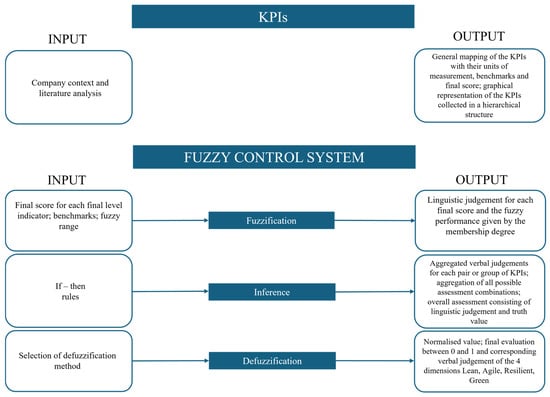
Figure 1. Methodological framework.

To facilitate its practical implementation, the following step-by-step process summarizes how the framework is implemented in Excel™, in alignment with the phases illustrated in Figure 1 and described in the following paragraphs:

• Data collection: Gather company-specific values for all selected KPIs, as listed in Table 1, and define the corresponding benchmark values.
  Table 1. List of KPIs from the LARG-related studies.

  Perspective	Indicator	Description
  Lean	Non-compliant supply quantity	Number of supplies that do not meet specified quality standards
  	Stock level (raw material)	Total quantity of raw materials available in stock
  	Inventory cost	Expenses associated with maintaining inventory, including storage, handling, and deterioration costs
  	Productivity	Measure of the efficiency in utilizing resources to produce goods or services
  	Production utilization capacity	Percentage of utilization of available production capacity
  	Overall equipment effectiveness	Percentage of time equipment operates effectively, considering availability, performance, and quality
  	Impact of set-up change on total production hours	Time spent on setup changes as a percentage of total production time
  	Operational production time	Actual time taken to produce one unit of product
  	Cycle time	Total time taken to complete a production cycle, from start to finish
  	Design time	Total time taken to design a new product or service
  	Development costs	Expenses incurred for developing new products or services
  	Inventory level (consumables and semi-finished products)	Total quantity of consumables and semi-finished materials available in inventory
  	Cost of rework and defects	Costs associated with reworking defective products and defect management
  	Material loss due to operations (transfer to another container)	Amount of material lost during operations, such as transfers and handling
  	Full truckload (FTL) vs. less-than-truckload (LTT)	Percentage of full-load deliveries compared to partial-load deliveries
  	Total order processing time	Total time required to fulfill an order, from receipt to delivery
  	Marketing cost	Expenses incurred to promote products or services
  	Average monthly sales	Average monthly sales
  	Sales effectiveness	Sales team’s ability to meet set targets
  	Profit margin on sales	Profit margin from sales after deducting costs
  	Inventory level (finished goods)	Total quantity of finished goods available in inventory
  	Customer satisfaction	Customer satisfaction level measured through surveys and feedback
  	Hours of training per year	Total number of training hours provided to employees in a year
  	Employees’ perception of the work environment	Employee satisfaction level with the work environment, measured through surveys
  Agile	Proximity to suppliers	Physical distance between the company and its suppliers, which can affect delivery times and transportation costs
  	Number of nodes in the supply chain	Number of steps or intermediaries a product goes through from production to final delivery
  	Supplier flexibility	Suppliers’ ability to quickly adapt to changes in demand or product specifications
  	Supplier lead time	Lead time between placing an order with the supplier and the actual delivery of materials or products
  	Supplier involvement in product development	Extent to which suppliers are actively involved in the design and development of new products
  	Flexibility of production mix	Production system’s ability to quickly switch from one product type to another without significant efficiency loss
  	Total production time	Total time taken to complete the production process of a product
  	Overtime hours	Number of overtime hours worked to complete production
  	Quantity of defective products	Quantity or percentage of products not meeting quality standards and requiring rework or disposal
  	Bottleneck quantity	Frequency or severity of bottlenecks in the production process that limit total production capacity
  	Delivery accuracy	Percentage of deliveries completed correctly compared to planned orders, with no errors
  	Delivery frequency (No. actual deliveries/ No. planned deliveries)	Ratio of actual deliveries to scheduled deliveries, an indicator of timeliness and reliability
  	On-time delivery	Measure of the ability to meet scheduled delivery times
  	Delivery flexibility	Ability to adjust delivery quantities and timing in response to changes in customer demand
  	Timeliness	Ability to respond quickly to market needs or changes in operating conditions
  	Speed of transforming inventory into sale	Time required to convert raw materials and work-in-progress into finished, sellable products
  	Inventory turnover ratio	Frequency with which inventory is sold and replenished over a period, indicating inventory management efficiency
  	Time to resolve the issue of the service request	Average time required to resolve an issue reported by customers or employees
  	Returns flexibility	Ability to effectively manage returns and service requests, including handling products from different sources or suppliers
  	Service Evaluation	Ability to maintain high service levels and responsiveness under changing customer demands or market conditions
  	Return request response time	Time required to respond to customer return requests
  Resilient	Supplier lead times	Average time taken by suppliers to fulfill an order from issuance to delivery
  	Supplier flexibility	Suppliers’ ability to adapt to changes in volumes and product mixes
  	Availability of alternative supplies	Ability to source alternative suppliers when needed
  	Inventory adjustment time	Time required to adjust inventory to new demand or supply conditions
  	Average time to preventive maintenance	Average time taken to perform preventive maintenance on equipment
  	Mean time between failures (MTBF)	Average time between two consecutive failures of a system during normal operation
  	Mean time to repair (MTTR)	Time required to restore system availability following an incident or outage.
  	Mean time to failures (MTTF)	The average time a non-repairable system operates before it fails.
  	Average downtime	Average downtime of a system or equipment
  	Number of reworked of modified	Quantity of products requiring rework or modification after initial production
  	Standardization of components	Degree of standardization of components used in products
  	Product customization	Ability to customize products to specific customer requirements
  	Breadth of product range	Diversity of products offered by the company
  	Resiliency of distribution channels	Ability of distribution channels to adapt to and recover from disruptions
  	Demand satisfaction	Ability to meet customer demand in terms of quantity and timing
  	Average customer seniority	Average customer retention time
  	Time to cover inventory	Period during which current inventory can meet forecasted demand
  	Safety Stock Quantity	Minimum stock level maintained to prevent disruptions in production or sales
  	Customer Retention Rate (CRR)	Percentage of customers remained over a specific time period
  	Number of lost sales	Number of lost sales due to stockouts or other issues
  	Customer satisfaction	Percentage of orders fully fulfilled based on available inventory
  Green	Cost of raw materials	Cost incurred for the purchase of raw materials required for production or service delivery
  	Use of renewable materials	Percentage of materials used that can be regenerated or recycled
  	Suppliers with environmental certifications	Suppliers with certifications attesting to environmentally sustainable practices
  	Water consumed	Total volume of water used in processes
  	Energy consumed produced from fossil and renewable resources	Total kW/MW of electricity used produced from renewable sources
  	Energy consumption	Total energy consumed in carrying out all activities
  	Human capital	Number of personnel required and involved in carrying out the activity
  	Waste index	Quantity of materials, resources, or products discarded during the production process
  	Compliant products	Products meeting the required quality standards
  	Number of smart tasks	Number of operations or processes performed using smart or automated technologies
  	Sanitation costs	Expenses incurred to ensure adequate hygiene and sanitary conditions within the company
  	CO2 emission	Total amount of carbon dioxide emitted from business activities
  	Fuel consumption	Total fuel consumed
  	Route efficiency	Delivery route efficiency based on factors such as real-time traffic
  	Vehicle load rate	Percentage of total load capacity utilization of vehicles
  	Cost of waste	Costs associated with the management and disposal of company-generated waste
  	Recycled packaging quantity	Amount of packaging materials used that can be recycled

• KPI scoring: Calculate the normalized score for each KPI, based on the company value and benchmark.
• Fuzzification: Convert the normalized KPI scores into linguistic terms (Very Low, Low, High, Very High) using trapezoidal membership functions.
• Hierarchical aggregation: Combine KPIs progressively according to the structure in Figure 2, using fuzzy if–then inference rules to obtain intermediate and final evaluations.
  

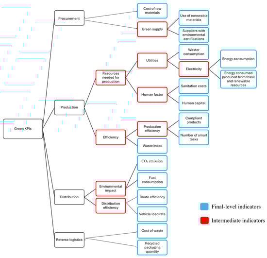  Figure 2. Example of a hierarchical aggregation structure for KPIs within the green dimension, used in the fuzzy logic framework.
• Truth value calculation: Determine the degree of truth for each rule-based output, reflecting the contribution of each KPI.
• Defuzzification and normalization: Aggregate the fuzzy outputs into a crisp score using the fuzzy mean method and normalization.
• Performance interpretation: Use the final values to interpret performance across the LARG dimensions and SC areas, identifying areas requiring improvement.

2.1. KPIs Definition

The first step in developing the fuzzy logic-based framework is the identification and definition of the relevant KPIs. These latter are carefully selected from the literature, focusing on the LARG paradigm, which serves as the basis for evaluating the supply chain. A total of 21 relevant studies were systematically reviewed to ensure a robust and comprehensive selection of indicators. The full list of references is provided in the additional material, available on the Mendeley Data repository at DOI: 10.17632/typfbkk3m8.1 [43]. Table 1 shows the KPIs with their description.

To ensure relevance and applicability in practice, the selected KPIs are to be aligned with the company’s specific performance metrics, which will be used to calculate the company’s values for each indicator.

The first output of this step is a general mapping of the KPIs along with their units of measurement and benchmark values, which helps compare the company’s performance against industry standards, best practices, or general (e.g., regulatory) benchmarks. In addition, the final score for each KPI is calculated in accordance with (1):

$$\mathrm{F}\mathrm{i}\mathrm{n}\mathrm{a}\mathrm{l}\mathrm{s}\mathrm{c}\mathrm{o}\mathrm{r}\mathrm{e}=\left\{\begin{array}{cc}{\displaystyle \frac{\mathrm{c}\mathrm{o}\mathrm{m}\mathrm{p}\mathrm{a}\mathrm{n}\mathrm{y} \mathrm{v}\mathrm{a}\mathrm{l}\mathrm{u}\mathrm{e}}{\mathrm{b}\mathrm{e}\mathrm{n}\mathrm{c}\mathrm{h}\mathrm{m}\mathrm{a}\mathrm{r}\mathrm{k}}}\times 100,& \mathrm{i}\mathrm{f} \mathrm{b}\mathrm{e}\mathrm{n}\mathrm{c}\mathrm{h}\mathrm{m}\mathrm{a}\mathrm{r}\mathrm{k}\ne 0\\ \mathrm{c}\mathrm{o}\mathrm{m}\mathrm{p}\mathrm{a}\mathrm{n}\mathrm{y} \mathrm{v}\mathrm{a}\mathrm{l}\mathrm{u}\mathrm{e},& \mathrm{i}\mathrm{f} \mathrm{b}\mathrm{e}\mathrm{n}\mathrm{c}\mathrm{h}\mathrm{m}\mathrm{a}\mathrm{r}\mathrm{k}=0\end{array}\right.$$

(1)

The second output of the first step is a graphical representation of the KPIs within a hierarchical structure, reflecting the relationships between individual indicators and their respective categories (procurement, production, distribution and reverse logistics) and subcategories.

2.2. Fuzzy Control System

The objective of fuzzy logic control (FLC) system is to control complex processes by means of human experience [44]. Indeed, it plays an important role when applied to complex phenomena that are not easily described by traditional mathematics [45]. In fuzzy set theory, trapezoidal fuzzy numbers are characterized by membership functions that increase monotonically from zero to one, remain constant, and then decrease monotonically back to zero, thus effectively modeling uncertainty with a clear structure. This monotonic behavior in the membership function is particularly useful in various engineering and decision-making applications, as it allows for a structured representation of uncertainty [46].

2.2.1. Fuzzification

In this phase, the input consists of the final scores calculated for each KPI, while the output includes both the corresponding linguistic evaluations and their fuzzy membership degrees.

To get a linguistic evaluation, each final score is mapped onto a four-point linguistic scale based on the model proposed by [47]. The linguistic terms used are: Very Low, Low, High, and Very High.

In this study, as in many other studies [48,49], trapezoidal functions are adopted to model the fuzzy numbers. The mathematical definition of a trapezoidal fuzzy number is expressed through membership function (2):

$$\mu \left(\mathrm{x}\right)=\left\{\begin{array}{cc}\hfill 0,& \mathrm{x}<\mathrm{a}\hfill \\ \hfill {\displaystyle \frac{\mathrm{x}-\mathrm{a}}{\mathrm{b}-\mathrm{a}}},& \mathrm{a}\le \mathrm{x}\le \mathrm{b}\hfill \\ \hfill 1,& \mathrm{b}\le \mathrm{x}\le \mathrm{c}\hfill \\ \hfill {\displaystyle \frac{\mathrm{x}-\mathrm{d}}{\mathrm{c}-\mathrm{d}}},& \mathrm{c}\le \mathrm{x}\le \mathrm{d}\hfill \\ \hfill 0,& \mathrm{x}>\mathrm{d}\hfill \end{array}\right.$$

(2)

where:

• x represents the numerical value of the variable (i.e., the final score against the selected KPI);
• µ(x) is the corresponding membership degree;
• a, b, c, and d are the parameters that define the shape of the trapezoidal fuzzy number, based on decision-makers’ judgment or benchmark tables.

As a result, this phase provides two outputs: the linguistic evaluation and the corresponding membership degree for each KPI.

2.2.2. Inference

The inference process is applied when indicators need to be aggregated, based on the hierarchical diagram previously described. This process relies on if-then rules to evaluate and combine the fuzzy sets of two or more indicators. In this case, aggregation is carried out between two indicators, as the hierarchical structure was designed to simplify calculations, although the method can be extended to more indicators if necessary.

The if-then rules used in the inference process are derived from semantic aggregation matrix based on linguistic combinations of input variables. They reflect expert knowledge since both the linguistic input values and the aggregation logic were developed in consultation with domain experts. This ensures that the inference process aligns with practical and contextual understanding.

The inference is based on a fuzzy rule matrix, such as the one shown in Table 2, where the fuzzy linguistic variables (e.g., Very low, Low, Average, High, Very high) are combined according to pre-defined rules. Each combination of input values from the two indicators results in an aggregated fuzzy value, which corresponds to the output linguistic value.

Table 2. Fuzzy inference rule matrix used to determine the output linguistic values.

	Very Low	Low	Average	High	Very High
Very low	Very low	Very low	Low	Low	Average
Low	Very low	Low	Low	Average	High
Average	Low	Low	Average	High	High
High	Low	Average	High	High	Very high
Very high	Average	High	High	Very high	Very high

In this matrix, the rows and columns represent the linguistic values of the two indicators being aggregated, and the intersection of each row and column gives the resulting output linguistic value.

In certain cases, it is appropriate to introduce a middle or neutral judgment (labeled as “Average”) during the aggregation process. This judgment is particularly useful in situations where the performance of the company with respect to two indicators is conflicting or shows intermediate levels of performance. The “Average” judgment helps better represent situations in which neither indicator significantly dominates the other, allowing for a more balanced assessment. This neutral value will be especially important for subsequent aggregations, where the results from multiple indicators are combined and evaluated.

The final output of the inference is the “truth value” of each indicator (Equation (3)).

$$\mathrm{T}\mathrm{r}\mathrm{u}\mathrm{t}\mathrm{h} \mathrm{v}\mathrm{a}\mathrm{l}\mathrm{u}\mathrm{e}={\prod }_{\mathrm{j}=1}^{\mathrm{i}}{\mu }_{\mathrm{j}}\left({\mathrm{x}}_{\mathrm{j}}\right)$$

(3)

In the formula above:

i: total number of KPIs considered

μ_j(x_j): membership degree of the j-th KPI

2.2.3. Defuzzification

The final step of the fuzzy control system involves defuzzification, a process in which the fuzzy output, known as the fuzzy set, is transformed into a crisp value. This step is essential in fuzzy logic systems to convert the qualitative results derived from inference rules into a usable, quantitative output. Therefore, the values obtained through defuzzification represent numerical equivalents of linguistic expressions that contain the system’s final assessment.

In general, this phase involves two key steps:

(i)

selecting the defuzzification method;

(ii)

normalizing the final score.

With respect to the first step, several defuzzification methods exist in the literature. Among them, the fuzzy mean (FM) method, highlighted by [50], is one of the most applied due to its simplicity and effectiveness. The FM method makes use of the following formula (Equation (4)):

$$\mathrm{F}\mathrm{M}={\displaystyle \frac{{\sum }_{\mathrm{k}=1}^{\mathrm{n}}{\mathrm{a}}_{\mathrm{k}}{\mathrm{X}}_{\mathrm{k}}}{{\sum }_{\mathrm{k}=1}^{\mathrm{n}}{\mathrm{a}}_{\mathrm{k}}}}$$

(4)

where:

• n is the number of fuzzy conclusions;
• a_k is the truth value (i.e., degree of membership) of the k-th conclusion obtained from the inference phase;
• X_k is the numeric value associated with the k-th conclusion. For trapezoidal fuzzy numbers, this is typically the average of the two values where the membership function reaches its maximum. Table 3 shows the fuzzy interval used to determine the X_k value.
  Table 3. Fuzzy ranges.

  Linguistic Judgment	a	b	c	d
  Very low	0.00	0.00	0.10	0.20
  Low	0.10	0.20	0.30	0.40
  Average	0.30	0.40	0.50	0.60
  High	0.50	0.60	0.70	0.80
  Very high	0.70	0.80	1.00	1.00

However, it is important to note that the crisp value and its range depend on the type of fuzzy numbers and linguistic scales adopted. Therefore, as a second step, a final normalization is required to express the output within a standardized range (typically between 0 and 1, with higher values indicating better performance). This is done using the following normalization formula (Equation (5)):

$$\mathrm{N}\mathrm{o}\mathrm{r}\mathrm{m}\mathrm{a}\mathrm{l}\mathrm{i}\mathrm{z}\mathrm{e}\mathrm{d} \mathrm{v}\mathrm{a}\mathrm{l}\mathrm{u}\mathrm{e}={\displaystyle \frac{(\mathrm{x}-\mathrm{m}\mathrm{i}\mathrm{n})}{(\mathrm{m}\mathrm{a}\mathrm{x}-\mathrm{m}\mathrm{i}\mathrm{n})}}$$

(5)

where:

• x is the crisp sustainability index before normalization;
• min and max are the minimum and maximum values in the possible range of variation, which correspond to the extreme cases where the company achieves the lowest or highest scores across all indicators.

3. Tool Implementation and Results

To demonstrate the applicability and effectiveness of the proposed fuzzy-based framework, a case study is presented. The tool is applied to a real company scenario in order to evaluate its supply chain performance across LARG perspective. This approach is consistent with other works in literature that have adopted case studies to test MCDM models in LARG context (e.g., [51,52,53]).

3.1. KPIs Definition

This step includes the “input interface” of the tool, including company’s value, unit of measurement, benchmark and final score, as described in the methodology section. For the sake of brevity, only the green dimension will be presented in this study (Table 4); even if the same methodology is applied for all the four dimensions (Appendix A, Table A1, Table A2 and Table A3).

Table 4. Company’s value, unit of measurement, benchmark and final score for green KPIs.

KPI Indicator	Company’s Value	Unit of Measure	Benchmark Type	Benchmark Value	Final Score
Cost of raw materials	65,000	Euro	Lower is better	–	65,000
Use of renewable materials	70	%	Higher is better	–	70.00%
Suppliers with environmental certifications	40	%	Best competitor	42	95.24%
Water consumption	95,000	Cubic meters per year	Lower is better	–	95,000
Energy consumed produced from fossil and renewable resources	25	%	[54]	32	78.13%
Energy consumption	17,000	MW per year	Lower is better	–	17,000
Human capital	150	Absolute number	Best competitor	170	88.24%
Waste index	5	%	Lower is better	–	5.00%
Compliant products	95	%	Higher is better	–	95.00%
Number of smart tasks	80	%	Higher is better	–	80.00%
Sanitation costs	22,000	Euro	Lower is better	–	22,000
CO2 emission	25,000	Kg CO2	Lower is better	–	25,000
Fuel consumption	520,000	Liters per year	Lower is better	–	520,000
Route efficiency	90	%	Higher is better	–	90%
Vehicle load rate	75	%	Higher is better	–	75%
Cost of waste	27,000	Euro	Lower is better	–	27,000
Recycled packaging quantity	70	%	[55]	65	107.69%

Figure 2 and Table 5 show a possible aggregation of the KPIs listed in Table 1 for the green dimension. The hierarchical structure of the remaining three perspectives is shown in Appendix A (Table A4, Table A5 and Table A6). Starting from the outermost part of the diagram, two final-level indicators are aggregated at a time, proceeding progressively inward until reaching the green category. This category represents the overall evaluation, which is derived from the indicators at the preceding levels. The diagram includes two types of indicators: those highlighted in blue represent the final-level indicators used for the assessment, while those highlighted in red are intermediate indicators required for the correct functioning of the tool according to the proposed logic. Although the graph represents the aggregation of two inputs at a time for simplicity, the proposed fuzzy approach is generalizable and can be extended to the aggregation of a larger number of inputs, depending on user requirements. The hierarchical structure used represents a methodological choice to ensure clarity, manageability, and scalability of the system without compromising the multi-criteria validity of the model. Again, this design is consistent with previous studies on fuzzy inference systems, which recommend hierarchical structures for reducing rule explosion and enhancing model interpretability in complex decision-making scenarios (e.g., [56,57]).

Table 5. Aggregation of green KPIs.

Level	KPI1	KPI2	Final Indicator
1	Energy consumed from fossil and renewable resources	Energy consumed	Electric energy
2	Water consumed	Electric energy	Utilities
2	Suppliers with environmental certifications	Use of renewable materials	Sustainable sourcing
2	Sanitation costs	Human capital	Human factor
2	Number of compliant products	Number of smart-performed activities	Production efficiency
3	Cost of raw materials	Sustainable sourcing	Procurement
3	Utilities	Human factor	Resources required for production
3	Waste index	Production efficiency	Efficiency
3	CO2 emission	Fuel consumption	Environmental impact
3	Route efficiency	Vehicle load rate	Distribution efficiency
3	Waste cost	Quantity of recyclable packaging	Reverse logistics
4	Resources required for production	Efficiency	Production
4	Environmental impact	Distribution efficiency	Distribution

3.2. Fuzzy Control System

3.2.1. Fuzzification

The first step, as described in the methodology, is the identification of linguistic judgment of each KPIs on the basis of their final score value. The fuzzy range of each green KPIs is defined and shown in Table 6. The fuzzy range of the remaining dimensions (lean, agile, resilient) are shown in Appendix B (Table A7, Table A8 and Table A9).

Table 6. Fuzzy range of green KPIs.

KPI	Linguistic Judgement	a	b	c	d
Use of renewable materials/Recycled packaging quantity/Energy consumed produced from fossil and renewable resources/Route efficiency/Human capital/Suppliers with environmental certifications/Number of smart tasks/Vehicle load rate/Compliant products	Very low	0%	0%	50%	55%
	Low	50%	55%	70%	75%
	High	70%	75%	88%	95%
	Very high	88%	95%	100%	100%
Fuel consumption	Very high	0	0	50,000	100,000
	High	50,000	100,000	150,000	200,000
	Low	150,000	200,000	300,000	400,000
	Very low	300,000	400,000	600,000	600,000
CO2 emission	Very high	0	0	10,000	15,000
	High	10,000	15,000	17,500	20,000
	Low	17,500	20,000	30,000	40,000
	Very low	30,000	40,000	80,000	80,000
Water consumption	Very high	0	0	25,000	30,000
	High	25,000	30,000	50,000	70,000
	Low	50,000	70,000	90,000	120,000
	Very low	90,000	120,000	200,000	200,000
Cost of waste	Very low	0	0	20,000	20,000
	Low	15,000	20,000	25,000	30,000
	High	25,000	30,000	35,000	40,000
	Very high	40,000	42,000	50,000	50,000
Cost of raw materials	Very low	0	0	100,000	200,000
	Low	100,000	200,000	300,000	400,000
	High	300,000	400,000	500,000	600,000
	Very high	500,000	600,000	1000.00	1000.00
Energy consumption	Very low	0	0	7000	9000
	Low	7000	9000	15,000	20,000
	High	15,000	20,000	25,000	30,000
	Very high	25,000	30,000	50,000	50,000
Sanitation costs	Very low	0	0	10,000	15,000
	Low	10,000	15,000	20,000	25,000
	High	20,000	25,000	30,000	35,000
	Very high	30,000	35,000	50,000	50,000
Waste index	Very high	0%	0%	50%	55%
	High	50%	55%	70%	75%
	Low	70%	75%	88%	95%
	Very low	88%	95%	100%	100%

On the basis of the fuzzy range and the final score, the linguistic judgment and the membership degree are defined, as shown in Table 7 and Appendix C (Table A10, Table A11 and Table A12).

Table 7. Linguistic judgment and membership degree of green KPIs.

KPIs	Linguistic Judgment	Membership Degree
Cost of raw materials	Very low	1
Use of renewable materials	Low	1
	High	0
Suppliers with environmental certifications	Very high	1
Water consumption	Low	0.83
	Very low	0.17
Energy consumed produced from fossil and renewable resources	High	1
Energy consumption	Low	0.6
	High	0.4
Human capital	High	0.97
	Very high	0.03
Waste index	Very high	1
Compliant products	High	0
	Very high	1
Number of smart tasks	High	1
Sanitation costs	Low	0.6
	High	0.4
CO2 emission	Low	1
Fuel consumption	Very low	1
Route efficiency	High	0.71
	Very high	0.29
Vehicle load rate	Low	0
	High	1
Cost of waste	Low	0.6
	High	0.4
Recycled packaging quantity	Very high	1

3.2.2. Inference

The KPIs are aggregated (see Table A13 in the Appendix D) to derive the final indicators, which include both the red values shown (subcategories) and the four main categories (Procurement, Production, Distribution, and Reverse Logistics), illustrated in Figure 2. Table 8 and Table A14, Table A15 and Table A16 in Appendix D report the inference results, providing the final truth values associated with each of these indicators, for green KPIs and other three dimensions, respectively.

Table 8. Inference results of green KPIs.

KPI	Final Judgement	Final Truth Value
Electricity	Average	0.6
	High	0.4
Utilities	Low	0.67
	Average	0.33
Sustainable procurement	High	1
	Very high	0
Human factor	Average	0.58
	High	0.41
	Very high	0.01
Production efficiency	High	0
	Very high	1
Procurement	Low	1
	Average	0
Resources required for production	Low	0.39
	Average	0.46
	High	0.15
Efficiency	Very high	1
Environmental impact	Very low	1
Distribution efficiency	Average	0
	High	0.71
	Very high	0.29
Reverse logistics	High	0.6
	Very high	0.4
Production	High	0.85
	Very high	0.15
Distribution	Low	0.71
	Average	0.29

3.2.3. Defuzzification

The goal of the tool is the achievement of a final assessment, broken down by process part, that encompasses the indicators initially selected in the final assessment. For each group of indicators Lean, Agile, Resilient and Green, the final evaluation formed by “linguistic judgment”, “truth value”, “fuzzy mean” and “final linguistic judgment” for Procurement, Production, Distribution and Reverse logistic is obtained (Table 9).

Table 9. Final evaluation by process part for each indicator group, expressed through linguistic judgment and truth value.

	Indicator	Truth Value	Xk	FM	Final Linguistic JudgmentI
Lean	Procurement	1	0.90	0.90	Very high
	Production	1	0.65	0.65	High
	Distribution	0	0.65	0.90	Very high
	Distribution	0	0.45
	Distribution	1	0.90
	Reverse Logistics	0	0.65	0.90	Very high
	Reverse Logistics	1	0.90
Agile	Procurement	0	0.15	0.25	Low
	Procurement	1	0.25
	Production	1	0.65	0.65	High
	Distribution	1	0.25	0.25	Low
	Reverse Logistics	0.49	0.90	0.77369338	Very high
	Reverse Logistics	0.51	0.65
Resilient	Procurement	1	0.90	0.90	Very high
	Production	1	0.90	0.90	Very high
	Distribution	0.83	0.65	0.65	High
	Distribution	0	0.45
	Reverse Logistics	0.56	0.65	0.761111111	Very high
	Reverse Logistics	0.44	0.90
Green	Procurement	1	0.25	0.25	Low
	Procurement	0	0.45
	Production	0.85	0.65	0.687255	High
	Production	0.15	0.90
	Distribution	0.71	0.25	0.307142857	Low
	Distribution	0.29	0.45
	Reverse logistics	0.6	0.65	0.75	Very high
	Reverse logistics	0.4	0.90

4. Discussion

Figure 3 shows the fuzzy mean and the final linguistic judgments for each dimension (lean, agile, resilient and green), divided by indicator (procurement, production, distribution and reverse logistic).

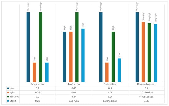
Figure 3. Final results—fuzzy mean and linguistic judgments of each dimension.

KPIs in the lean dimension show very high performance in any activity: procurement, distribution and reverse logistics have fuzzy mean equal to 0.9, with a linguistic judgment equal to “very high”; while production has a fuzzy mean equal to 0.65 and a linguistic judgment equal to “high”.

The agile perspective shows a very heterogeneous distribution: procurement and distribution show low values (FM = 0.25, ratings “low” linguistic judgment), while Production reaches a FM of 0.65 (“high”) and reverse logistics stands out with a FM of 0.77 (“very high”). As for Resilience, the results are more homogeneous: Procurement and Production reach FM values equal to 0.90 (“very high”), distribution has FM equal to 0.65 (“high”), while Reverse Logistics stands at 0.76 (“very high”).

Finally, the Green dimension highlights high values for production (around 0.68) and reverse logistics (0.75); while procurement and distribution have “low” values, around 0.25 and 0.31 respectively.

4.1. Theoretical Implications

From a theoretical perspective, the model evaluated by the fuzzy approach contributes to the literature on LARG supply chain.

The results highlight several theoretical insights:

• Lean activities emerge as a consolidated operational foundation across all supply chain phases. Consistent with their historical role in ensuring efficiency and standardization.
• Agility, despite being traditionally conceptualized as a transversal capability, appears to be strongly localized in specific operational areas.
• Resilience, recognized as a strategy to optimize and maintain the efficiency of the supply chain activities during disruptions events, proves to be a structural requirement.
• Finally, the data related to the green dimension support the theoretical hypothesis according to which sustainability practices are more easily implemented within business processes, confirming that internal management represents a key factor in the adoption of such practices [58]. On the contrary, the integration of sustainability in supplier relations and in downstream distribution is more complex and presents greater critical issues.

4.2. Managerial Considerations

This study not only signal vulnerabilities but also provides insights that can support managerial decisions in different areas of the supply chain. The LARG framework, assessed through the implementation of the tool, highlights how each dimension (lean, agile, resilient and green) is perceived and implemented in practice, offering indications on where to strengthen and/or improve strategic efforts.

Given the consistently high performance, lean practices appear to be well integrated and standardized. In production, however, where performance is relatively lower, there may be the necessity to strengthen lean initiatives through increased standardization, reduced variability and continuous improvement practices.

The heterogeneous performance of the agile dimension suggests that agility is not uniformly embedded across the supply chain. While agility in reverse logistics and production is strong, its limited presence in procurement and distribution means that the company may not be able to adapt in time when the market changes suddenly or when supply issues arise. Managers should consider investing in digital tools (e.g., real-time monitoring, demand forecasting) and flexible sourcing strategies to improve agility, especially in procurement and distribution.

High performance in procurement and manufacturing highlights that upstream resilience has become a structural priority, likely in response to recent global crises. Managers should maintain this focus by developing strong supplier relationships; at the same time, efforts should be made to extend resilience downstream, particularly in distribution, where the capacity to handle disruptions appears relatively weaker.

The green dimension shows a clear distinction between internal (i.e., production and reverse logistics) and external (i.e., procurement and distribution) operations. Managers should leverage positive results in production and reverse logistics, using these successes as a basis for spreading more sustainable practices through the company. However, low scores in procurement and distribution signal a need for greater involvement of green suppliers and more sustainable solutions, such as sustainability criteria in supplier selection [29] and partnerships with green logistics providers.

Based on these findings, the following managerial considerations can be drawn:

• Maintain lean practices as standardized routines and extend them to production activities, for which the current performance is lower.
• Invest in standardization, value stream mapping and continuous improvement to strengthen lean performance in production.
• Invest in flexible transport options or demand forecasting technologies to enhance agile distribution performance.
• Enhance supply chain responsiveness by adopting flexible procurement policies, improving demand sensing and integrating real-time monitoring tools.
• Develop downstream resilience through improved distribution flexibility, last-mile risk mitigation and crisis response planning.
• Promote green supplier development, introduce sustainability criteria in procurement and partner with green logistics providers to close the internal-external performance gap.

4.3. Practical Implications

This study provides insights for supply chain managers by showing how lean, agile, resilient and green dimensions are perceived and implemented across different operational areas, namely procurement, production, distribution and reverse logistics. The breakdown of results by process allows for a more precise understanding of where strengths and weaknesses lie, support targeted interventions rather than generalized strategies. By relying on objective data rather than assumptions, managers can make more informed decisions, identify strengths and weaknesses, and implement targeted corrective actions. The proposed tool is also highly adaptable and can be applied to any type of company or supply chain context. To ensure its effectiveness, it is essential that the decision-makers or user customizes the assessment by developing specific reference tables for each indicator. These must be based on the user’s knowledge and experience of the company being analyzed, ensuring that the assessment reflects the unique characteristics and strategic priorities of the organization. Moreover, the Excel^TM implementation offers accessibility, transparency and ease use.

5. Conclusions

Moving from a previous study [42] which developed a preliminary AHP-based framework for evaluating supply chains through LARG perspectives and highlighted the need to explore additional decision-making approaches alongside AHP, as well as suggesting that computerizing the tool via apps or technological solutions could enhance its applicability for companies, this study aims to create a fuzzy logic-based framework for LARG supply chain evaluation and implement the tool using Excel^TM.

The developed framework allows to accurately analyze the supply chain performance along its internal (i.e., production and reverse logistics) and external (i.e., procurement and distribution) activities and along the four LARG dimensions, offering a concrete basis for continuous improvement strategies. It provides a solid foundation for identifying inefficiencies, addressing critical issues through targeted interventions, and ultimately enhancing competitiveness, sustainability, and adaptability.

Additionally, the fuzzy logic framework developed in this study is particularly suited for addressing various types of uncertainty commonly encountered in supply chain decision-making. By structuring the evaluation across four operational areas (procurement, production, distribution, and reverse logistics), the model captures specific uncertainty factors tied to each domain. In procurement, it accounts for supplier lead time variability, reliability, and flexibility, which are often unpredictable. In production, the model handles variability in equipment effectiveness, process times, and defect rates, helping mitigate risks tied to capacity constraints or operational disruptions. In distribution, uncertainties in delivery accuracy, load efficiency, and fuel consumption are integrated into the analysis, supporting better logistics planning under fluctuating demand conditions. Finally, in reverse logistics, the model incorporates uncertainties linked to return flow timing, volume, and processing efficiency, which are typically hard to forecast. By translating qualitative and variable data into fuzzy linguistic terms, the model enables a more flexible and realistic evaluation under incomplete or ambiguous information, aligning with the complex and dynamic nature of real-world supply chains.

However, some limitations must be acknowledged. The list of indicators considered in this study is intended to represent a flexible starting point for company-level assessments, but it does not constitute an exhaustive or universally valid framework. It must be adapted and updated according to the specific context in which the tool is applied. Similarly, although the hierarchical structure (Figure 2) illustrates the aggregation of two KPIs for simplicity, the model is fully scalable and can handle a higher number of inputs as needed. Due to the high variability among companies, in terms of industry, market and organizational structure, it is not possible to define general fuzzification scales. These scales must be customized each time the tool is applied to a new company or each time new KPIs are introduced into the evaluation framework. Based on the above, the numerical results pointed out in this study are related to this specific context and can’t be considered as universally valid; but the full potential of this model lies in its adaptability.

The implementation of the framework in Excel^TM offers some advantages, as the software package is user-friendly (especially for practitioners unfamiliar with advanced programming tools), accessible in almost any company and generally suitable for small to medium instances of decision-making problems [59,60]. Nonetheless, from a technical point of view, it could present some limits in terms of computational power, scalability and integration with enterprise information systems. Future applications may benefit from shifting the tool to more robust platforms (e.g., MATLAB, Phyton-based framework or cloud-based solutions), which would allow for enhanced data processing, automation and real-time integration with other decision support systems.

To further validate the proposed framework and verify the robustness of the applied approach, future research could also incorporate comparative analyses. These may include benchmarking the tool against alternative MCDM techniques, as well as testing the effectiveness of the approach in a different organizational setting.

Finally, although the current study relies on a single case application, similarly to other contributions in LARG-MCDM literature, future research should expand the testing of the model across multiple industries and compare its performance with alternative tools and frameworks.

References

- Lotfi, M.; Saghiri, S. Disentangling resilience, agility and leanness: Conceptual development and empirical analysis. J. Manuf. Technol. Manag. 2018, 29, 168–197. [Google Scholar] [CrossRef]
- Jha, P.; Ghorai, S.; Jha, R.; Datt, R.; Sulapu, G.; Singh, S. Forecasting the impact of epidemic outbreaks on the supply chain: Modelling asymptomatic cases of the COVID-19 pandemic. Int. J. Prod. Res. 2023, 61, 2670–2695. [Google Scholar] [CrossRef]
- Azevedo, S.; Carvalho, H.; Cruz-Machado, V. A proposal of LARG supply chain management practices and a performance measurement system. Int. J. e-Educ. e-Bus. e-Manag. e-Learn. 2011, 1, 7–14. [Google Scholar] [CrossRef]
- Ohno, T. The Toyota Production System; Productivity Press: Portland, OR, USA, 1998. [Google Scholar]
- Womack, J.; Jones, D.; Roos, D. The Machine That Change the World; HarperCollins Publisher: New York, NY, USA, 1991. [Google Scholar]
- Reichhart, A.; Holweg, M. Lean distribution: Concepts, contributions, conflicts. Int. J. Prod. Res. 2007, 45, 3699–3722. [Google Scholar] [CrossRef]
- Parveen, M.; Rao, T. An integrated approach to design and analysis of lean manufacturing system: A perspective of lean supply chain. Int. J. Serv. Oper. Manag. 2009, 5, 175–208. [Google Scholar] [CrossRef]
- Melton, T. The benefits of lean manufacturing: What lean thinking has to offer the process industries. Chem. Eng. Res. Des. 2005, 83, 662–673. [Google Scholar] [CrossRef]
- Agarwal, A.; Shankar, R.; Tiwari, M.K. Modeling agility of supply chain. Ind. Mark. Manag. 2007, 36, 443–457. [Google Scholar] [CrossRef]
- Christopher, M. The agile supply chain: Competing in volatile markets. Ind. Mark. Manag. 2000, 29, 37–44. [Google Scholar] [CrossRef]
- Baramichai, M.; Zimmers, E.W., Jr.; Marangos, C.A. Agile supply chain transformation matrix: An integrated tool for creating an agile enterprise. Supply Chain Manag. Int. J. 2007, 12, 334–348. [Google Scholar] [CrossRef]
- Swafford, P.M.; Ghosh, S.; Murthy, N. Achieving supply chain agility through IT integration and flexibility. Int. J. Prod. Econ. 2008, 116, 288–297. [Google Scholar] [CrossRef]
- Goldsby, T.J.; Griffis, S.E.; Roath, A.S. Modeling lean, agile, and leagile supply chain strategies. J. Bus. Logist. 2006, 27, 57–80. [Google Scholar] [CrossRef]
- Haimes, Y.Y. On the definition of vulnerabilities in measuring risks to infrastructures. Risk Anal. Int. J. 2006, 26, 293–296. [Google Scholar] [CrossRef] [PubMed]
- Rice, J.B.; Caniato, F. Building a secure and resilient supply network. Supply Chain. Manag. Rev. 2003, 7, 22–30. [Google Scholar]
- Hansson, S.O.; Helgesson, G. What is stability? Synthese 2003, 136, 219–235. [Google Scholar] [CrossRef]
- Tang, S. Robust strategies for mitigating supply chain disruptions. Int. J. Logist. Res. Appl. 2006, 9, 33–45. [Google Scholar] [CrossRef]
- Christopher, M.; Peck, H. Building the resilient supply chain. Int. J. Logist. Manag. 2004, 15, 1–13. [Google Scholar] [CrossRef]
- Iakovou, E.; Vlachos, D.; Xanthopoulos, A. An analytical methodological framework for the optimal design of resilient supply chains. Int. J. Logist. Econ. Glob. 2007, 1, 1–20. [Google Scholar] [CrossRef]
- Rao, P.; Holt, D. Do green supply chains lead to competitiveness and economic performance? Int. J. Oper. Prod. Manag. 2005, 25, 898–916. [Google Scholar] [CrossRef]
- Carvalho, H.; Govindan, K.; Azevedo, S.G.; Cruz-Machado, V. Modelling green and lean supply chains: An eco-efficiency perspective. Resour. Conserv. Recycl. 2017, 120, 75–87. [Google Scholar] [CrossRef]
- Mathiyazhagan, K.; NoorulHaq, A.; Geng, Y. An ISM approach for the barrier analysis in implementing green supply chain management. J. Clean. Prod. 2013, 47, 283–297. [Google Scholar] [CrossRef]
- Sharma, V.; Raut, R.D.; Mangla, S.K.; Narkhede, B.E.; Luthra, S.; Gokhale, R. A systematic literature review to integrate lean, agile, resilient, green and sustainable paradigms in the supply chain management. Bus. Strategy Environ. 2021, 30, 1191–1212. [Google Scholar] [CrossRef]
- Ding, J.; Chen, X.; Sun, H.; Yan, W.; Fang, H. Hierarchical structure of a green supply chain. Comput. Ind. Eng. 2021, 157, 107303. [Google Scholar] [CrossRef]
- Dehghan-Bonari, M.; Bakhshi, A.; Aghsami, A.; Jolai, F. Green supply chain management through call option contract and revenue-sharing contract to cope with demand uncertainty. Clean. Logist. Supply Chain. 2021, 2, 100010. [Google Scholar] [CrossRef]
- Piotrowicz, W.; Cuthbertson, R. Performance measurement and metrics in supply chains: An exploratory study. Int. J. Product. Perform. Manag. 2015, 64, 1068–1091. [Google Scholar] [CrossRef]
- Prakongwittaya, S.; Liangrokapart, J. Integrating LARG measures to improve supply chain transparency performance. Asia Pac. Manag. Rev. 2025, 30, 100324. [Google Scholar] [CrossRef]
- Chand, M.; Raj, T.; Shankar, R. A comparative study of multi criteria decision making approaches for risks assessment in supply chain. Int. J. Bus. Inf. Syst. 2015, 18, 67–84. [Google Scholar] [CrossRef]
- Bottani, E.; Di Nardo, M.; Monferdini, L.; Murino, T. Mapping LARGS criteria and relationships for supplier selection using a fuzzy hybrid approach. Comput. Ind. Eng. 2025, 206, 111252. [Google Scholar] [CrossRef]
- Bhushan, N.; Rai, K. In Strategic decision making: Applying the analytic hierarchy process. In The Analytic Hierarchy Process; Springer: London, UK, 2004; pp. 11–21. [Google Scholar]
- Dutta, P.; Konwar, A. Multicriteria decision making analysis based on Fermatean fuzzy distance measure and entropy measure with application in COVID-19. Pattern Anal. Appl. 2025, 28, 1–32. [Google Scholar] [CrossRef]
- Govindan, K.; Azevedo, S.G.; Carvalho, H.; Cruz-Machado, V. Lean, green and resilient practices influence on supply chain performance: Interpretive structural modeling approach. Int. J. Environ. Sci. Technol. 2015, 12, 15–34. [Google Scholar] [CrossRef]
- Azevedo, S.G.; Carvalho, H.; Cruz-Machado, V. LARG index: A benchmarking tool for improving the leanness, agility, resilience and greenness of the automotive supply chain. Benchmarking Int. J. 2016, 23, 1472–1499. [Google Scholar] [CrossRef]
- Jamali, G.; Asl, E.K.; Zolfani, S.H.; Šaparauskas, J. Analysing LARG Supply Chain Management Competitive Strategies in Iranian Cement Industries. Bus. Adm. Manag. 2017, 1, 70–83. [Google Scholar]
- Mohamadi Zanjiran, D.; Hashemkhani Zolfani, S.; Prentkovskis, O. LARG supplier selection based on integrating house of quality, Taguchi loss function and MOPA. Econ. Res.-Ekon. Istraz. 2019, 32, 1944–1964. [Google Scholar]
- Divsalar, M.; Ahmadi, M.; Nemati, Y. A SCOR-Based Model to Evaluate LARG Supply Chain Performance Using a Hyrid MADM Method. IEEE Trans. Eng. Manag. 2020, 69, 1101–1120. [Google Scholar] [CrossRef]
- Sheykhizadeh, M.; Ghasemi, R.; Vandchali, H.R.; Sepehri, A.; Torabi, S.A. A hybrid decision-making framework for a supplier selection problem based on lean, agile, resilience, and green criteria: A case study of a pharmaceutical industry. Environ. Dev. Sustain. 2024, 26, 30969–30996. [Google Scholar] [CrossRef]
- Kabadayi, N.; Bakkal, S. Fermatean Fuzzy Analytic Hierarchy Process for Supplier Selection on LARG Supply Chain Paradigm. In International Conference on Intelligent and Fuzzy Systems; Springer: Berlin/Heidelberg, Germany, 2024. [Google Scholar]
- Espadinha-Cruz, P.; Grilo, A.; Cruz-Machado, V. Fuzzy evaluation model to assess interoperability in LARG Supply Chains. In Proceedings of the 9th International Conference on Fuzzy Systems and Knowledge Discovery, Chongqing, China, 29–31 May 2012. [Google Scholar]
- Amjad, M.S.; Rafique, M.Z.; Khan, M.A. Modern divulge in production optimization: An implementation framework of LARG manufacturing with Industry 4.0. Int. J. Lean Six Sigma 2021, 12, 992–1016. [Google Scholar] [CrossRef]
- Raut, R.D.; Mangla, S.K.; Narwane, V.S.; Dora, M.; Liu, M. Big Data Analytics as a mediator in Lean, Agile, Resilient, and Green (LARG) practices effects on sustainable supply chains. Transp. Res. Part E Logist. Transp. Rev. 2021, 145, 102170. [Google Scholar] [CrossRef]
- Bottani, E.; Monferdini, L.; Casella, G.; Mora, C. Evaluating Supply Chain Performance Through Lean, Agile, Resilient, and Green (LARG) Perspectives: A Comprehensive Framework. In Proceedings of the 21st International Multidisciplinary Modeling and Simulation Multiconference, I3M 2024, I3M Conference, Tenerife, Spain, 18–20 September 2024. [Google Scholar]
- Monferdini, L.; Casella, G.; Bottani, E. Studies Related to LARG Supply Chain. Mendeley Data. 2025, V1. Available online: https://data.mendeley.com/datasets/typfbkk3m8/1 (accessed on 8 July 2025).
- Zimmermann, H. Fuzzy Control. In Fuzzy Set Theory—And Its Applications; Springer: Dordrecht, The Netherlands, 2001. [Google Scholar]
- Pourjavad, E.; Shahin, A. The Application of Mamdani Fuzzy Inference System in Evaluating Green Supply Chain Management Performance. Int. J. Fuzzy Syst. 2018, 20, 901–912. [Google Scholar] [CrossRef]
- Allahviranloo, T.; Jahantigh, M.A.; Hajighasemi, S. A new distance measure and ranking method for generalized trapezoidal fuzzy numbers. Math. Probl. Eng. 2013, 1, 623757. [Google Scholar] [CrossRef]
- Chen, T.-Y.; Ku, T.-C. Importance-Assessing Method with Fuzzy Number-Valued Fuzzy Measures and Discussions on TFNs and TrFNs. Int. J. Fuzzy Syst. 2008, 10, 92–103. [Google Scholar]
- Kaur, A.; Kumar, A. A new method for solving fuzzy transportation problems using ranking function. Appl. Math. Model. 2011, 35, 5652–5661. [Google Scholar] [CrossRef]
- Nieto-Morote, A.; Ruz-Vila, F. A fuzzy approach to construction project risk assessment. Int. J. Proj. Manag. 2011, 29, 220–231. [Google Scholar] [CrossRef]
- Van Leekwijck, W.; Kerre, E.E. Defuzzification: Criteria and classification. Fuzzy Sets Syst. 1999, 108, 159–178. [Google Scholar] [CrossRef]
- Azevedo, S.G.; Govindan, K.; Carvalho, H.; Cruz-Machado, V. Ecosilient Index to assess the greenness and resilience of the upstream automotive supply chain. J. Clean. Prod. 2013, 56, 131–146. [Google Scholar] [CrossRef]
- Sahu, K.; Sharma, M.; Raut, R.D.; Sahu, A.K.; Sahu, N.K.; Antony, J.; Tortorella, G.L. Decision-making framework for supplier selection using an integrated MCDM approach in a lean-agile-resilient-green environment: Evidence from Indian auautomotive sector. TQM J. 2023, 35, 964–1006. [Google Scholar] [CrossRef]
- Akbarzadeh, Z.; Ghadikolaei, A.S.; Madhoushi, M.; Aghajani, H. A hybrid fuzzy multicriteria decision making model based on fuzzy DEMATEL with fuzzy analytical network process and interpretative structural model prioritizing LARG supply chain practices. Int. J. Eng. 2019, 32, 413–423. [Google Scholar]
- Directive (EU) 2018/2001; Directive (EU) 2018/2001, of the European Parliament and of the Council on the Promotion of the Use of Energy from Renewable. Official Journal of the European Union: Brussels, Belgum, 2018.
- DIRECTIVE 94/62/EC; European Parliament and Council Directive 94/62/EC on Packaging and Packaging Waste. Official Journal of European Union: Brussels, Belgum, 1994.
- Zhang, X.; Onieva, E.; Perallos, A.; Osaba, E.; Lee, V.C. Hierarchical fuzzy rule-based system optimized with genetic algorithms for short term traffic congestion prediction. Transp. Res. Part C Emerg. Technol. 2014, 43, 127–142. [Google Scholar] [CrossRef]
- Kamthan, S.; Singh, H. Hierarchical Fuzzy Logic Systems. J. Inst. Eng. India Ser. B 2022, 103, 1167–1175. [Google Scholar] [CrossRef]
- Li, X.; Liu, D.; Zhang, Z.; Cheng, T.; Liu, L.; Yuan, J. The impact of internal and external green supply chain management activities on performance improvement: Evidence from the automobile industry. Heliyon 2022, 8, e11486. [Google Scholar] [CrossRef] [PubMed]
- Hesse, R.; Scerno, D.H. How electronic spreadsheets changed the world. Interfaces 2009, 39, 159–167. [Google Scholar] [CrossRef]
- Bottani, E.; Montanari, R.; Rinaldi, M. Development and testing of software tool for warehouse design and picking optimization. Int. J. Manag. Decis. Mak. 2019, 18, 119–150. [Google Scholar] [CrossRef]
Disclaimer/Publisher’s Note: The statements, opinions and data contained in all publications are solely those of the individual author(s) and contributor(s) and not of MDPI and/or the editor(s). MDPI and/or the editor(s) disclaim responsibility for any injury to people or property resulting from any ideas, methods, instructions or products referred to in the content. |
© 2025 by the authors. Licensee MDPI, Basel, Switzerland. This article is an open access article distributed under the terms and conditions of the Creative Commons Attribution (CC BY) license (https://creativecommons.org/licenses/by/4.0/).