Apis mellifera Bee Verification with IoT and Graph Neural Network

Abstract

Automatic recognition systems (ARS) have been proposed in scientific and technological research for the care and preservation of endangered species; these systems, consisting of Internet of Things (IoT) devices and object-recognition techniques with artificial intelligence (AI), have emerged as proposed solutions to detect and prevent parasite attacks on Apis mellifera bees. This article presents a pilot ARS for the recognition and analysis of honeybees at the hive entrance using IoT devices and automatic object-recognition techniques, for the early detection of the Varroa mite in test apiaries. Two object-recognition techniques, namely the k-Nearest Neighbor Algorithm (kNN) and Graph Neural Network (GNN), were evaluated with an image dataset of 600 images from a single beehive. The results of the experiments show the viability of using GNN in real environments. GNN has greater accuracy in bee recognition, but with greater processing time, while the kNN classifier requires fewer processing resources but has lower recognition accuracy.

1. Introduction

The preservation and care of endangered species is an ongoing concern for different sectors of society; the bee Apis mellifera, or the honeybee, is not exempt from risks of extinction for different reasons [1]. One of these is attack and invasion by the Varroa mite, which has caused ongoing concern among beekeepers and environmentalists, and is capable of devastating entire colonies of bees where they nest [2,3,4,5,6]. The Varroa mite has been identified as the most destructive ectoparasite of the honeybee [2]. It is considered one of the greatest biological threats to the health of bees [6], and can cause the inability of foraging bees to fly, disorientation, paralysis, and the death of individuals in the colony [7]. The prevalence of this mite has been studied in agro-ecological regions of different countries [3,4]. The presence and effects of the Varroa mite in hives where they infect and destroy honeybees has been analyzed and studied in different areas of scientific and technological research [2,3]; however, despite the efforts made by insecticides, acarologists and beekeepers have not yet produced long-term solutions for the control of Varroa [6]. Proposed alternative techniques, such as the development of better beekeeping practices [5], integrated pest management (IPM) [6], international monitoring, and therapeutic alternatives [7], all seek to increase the effectiveness of Varroa mite control.

Currently, the Varroa mite is detected by beekeepers through two types of visual checks [8,9], double-sieve sampling and powdered sugar sampling. Both checks have been documented by the Food and Agriculture Organization of the United Nations (FAO) [10]. When carried out in apiaries, both of these checks imply the opening of the hive at a time that the beekeeper decides. After the hive is open, hundreds of bees are collected and killed with isopropyl alcohol, then discarded with filters that show the existence or absence of the Varroa ectoparasite [8,9,11]. The manual collection of the ectoparasite [12] using substances applied to a group of approximately 100 bees allows for the detection of the infestation in the hive. If the ectoparasite is detected, the application of effective acaricides (fluvalinate-tau, coumaphos, or mitraz) [7] is carried out. Another method for detecting the Varro mite, in [11], is a visual analysis of the hive followed by the detection and counting of the number of mites on a sliding unit, then the estimation of the possible level of infestation by a heuristic calculation from the count.

These controls have three main disadvantages: first, they cause stress, loss of the queen, and loss of larvae in gestation in the colony due to the opening of the hive; second, every time manual control of the Varroa mite is carried out, hundreds of productive-age bees are sacrificed in each hive; and third, the effectiveness of the control is questionable, as it is based solely on the periodicity of the controls carried out by the beekeeper in the apiary. Thus, if few visual controls are carried out per year, the risk of attack by the Varroa mite increases; contrary to the above, however, if many controls are carried out, the risk of stress, escape of queens, and damage to larvae (unborn bees) increases.

The automation of the Varroa mite verification procedures in hives is a feasible development of an automatic recognition systems (ARS). Automatic recognition systems (ARS) consisting of intelligent software systems that manipulate miniaturized electrical, electronic, and mechanical devices, have emerged as an alternative to manual visual inspections. Pattern-recognition methods that allow for automated visual analysis have proven effective in different areas of scientific research. In the search for solutions to the Varroa ectoparasite, several works have been proposed [8,9,13,14,15,16,17,18,19,20,21,22]. These works are focused on the development of computer systems for the detection and reduction of the harmful effects of the Varroa ectoparasite with different analysis and object-recognition techniques in images applied in real environments.

For the development of automatic recognition systems, three areas of research must be considered: first, the real environment where the system must operate; second, the use of digital image-processing techniques to extract image features; and finally, the methods of object recognition in the images. We refer to each of the areas below according to the research work carried out in visual-inspection systems in apiaries.

Real environments have a certain degree of complexity when implementing computer systems for outdoor environments, as the images are influenced by different factors such as lighting, the area of the real environment, and the movement of objects [15,23], as well as data-processing speeds greater than conventional ones [24]. Digital image-processing techniques for the identification of regions and extraction of object features from the image [25], have been successfully used in automatic recognition systems; in this way, these techniques are used in systems applied to video inspection in beehives. For example, ref. [14] measured activity at the hive entrance by processing a set of frames, ref. [15] detected pollen-carrying bees, parasites were detected in [8], and Varroa mites were detected in [9,19,20,21,22].

In bee surveillance systems, two methods have been used for recognition: Gaussian [14,15] and neural networks [8,15,21,22]. The neural-network models that have been used successfully have been the following: ref. [9] used a pre-trained Convolutional Neural Network (CNN) model to detect bees; ref. [20] used YOLO with a single neural network to predict bounding boxes; ref. [21] used a Convolutional Neural Network for bee detection and Varroa identification, and ref. [22] used a deep-learning model based on Faster CNN (R-CNN) architecture to perform Varroa mite detection.

A different neural-network model from the previous ones is the Graph Neural Network (GNN) initially proposed in [26]; this type of network represents, in a natural way and through graph structures, various application areas [27]. GNNs for object recognition in images are being widely used. For example, in [28,29] they are used for image classification; in [30], edge features extracted from objects contained in images are used in object recognition with GNNs; in [31], GNNs are used for extracting planar roof structures from high-resolution images; in [32], GNNs are used for symbol detection in document images. GNN applications are not only limited to applications in images; they have also been used for graph learning representation [33].

Although various neural-network models have been applied to the detection of Varroa mites in bees, the problem remains open. Then, considering the examples from the analyzed literature and the problem of the Varroa mite existing in the environment, in addition to the traditional practices of Varroa mite control (both described in the previous paragraphs), we propose in this research work the development of a noninvasive visual-inspection system, retaining the standards of care of bees, which can remain in an apiary for an indefinite period of time, performing the tasks of detecting the Varroa parasite.

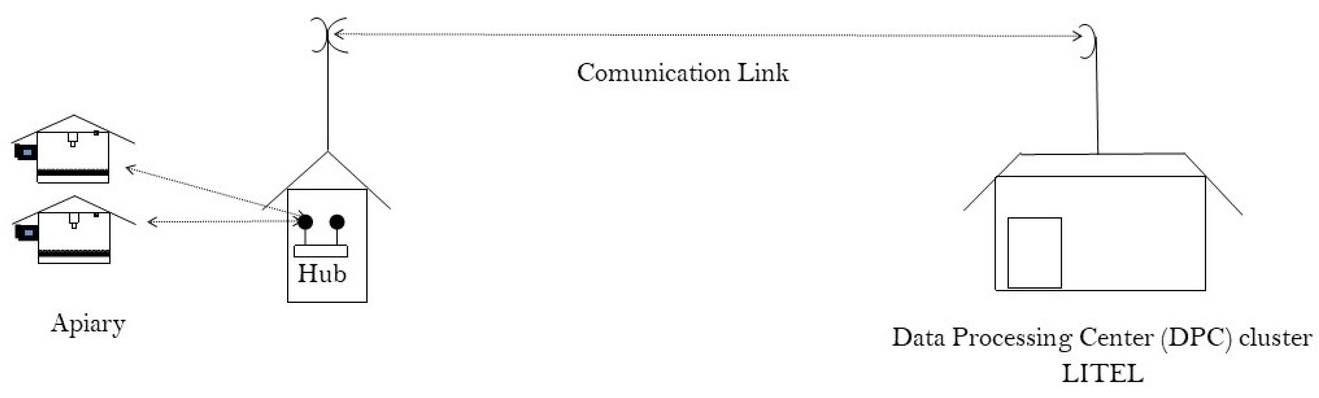
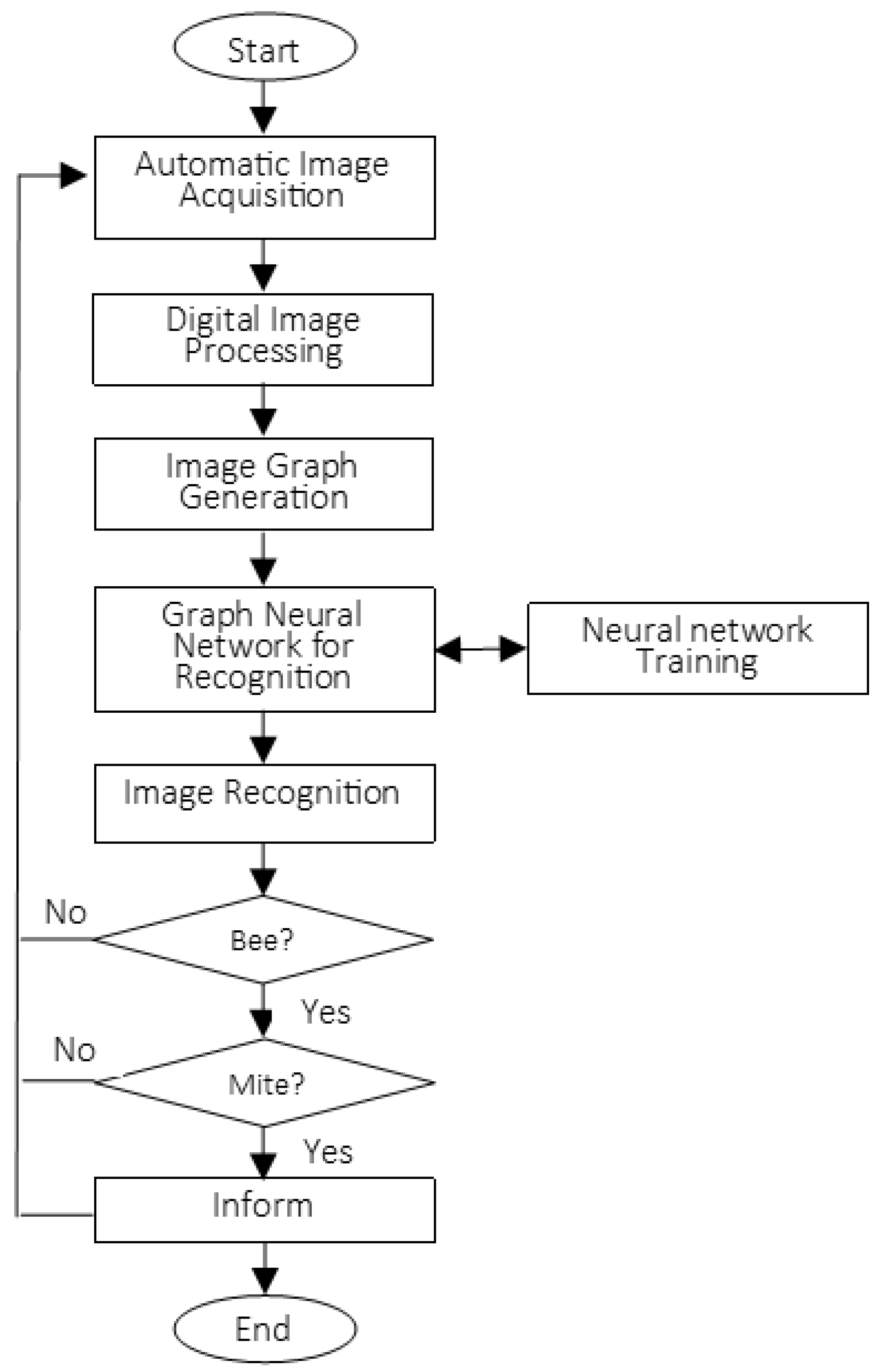
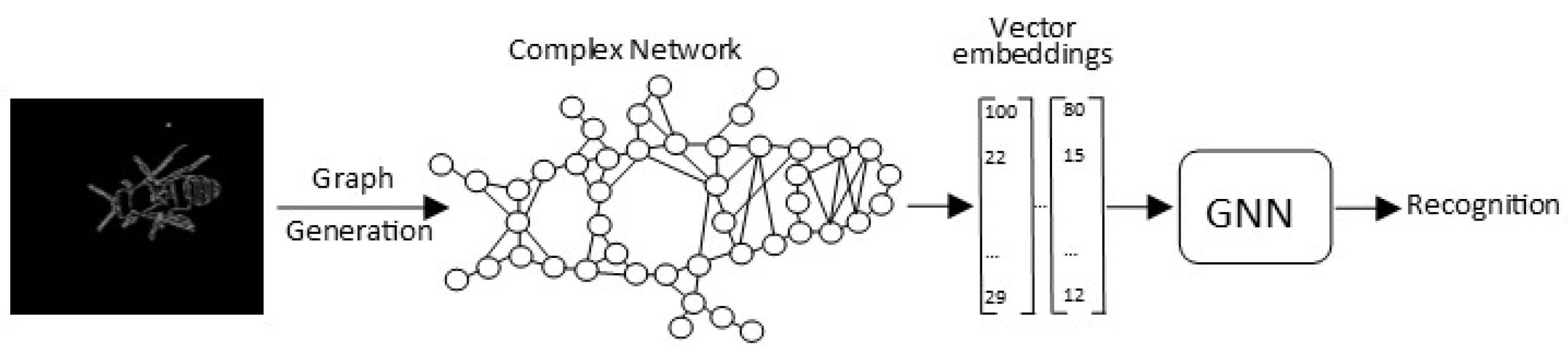
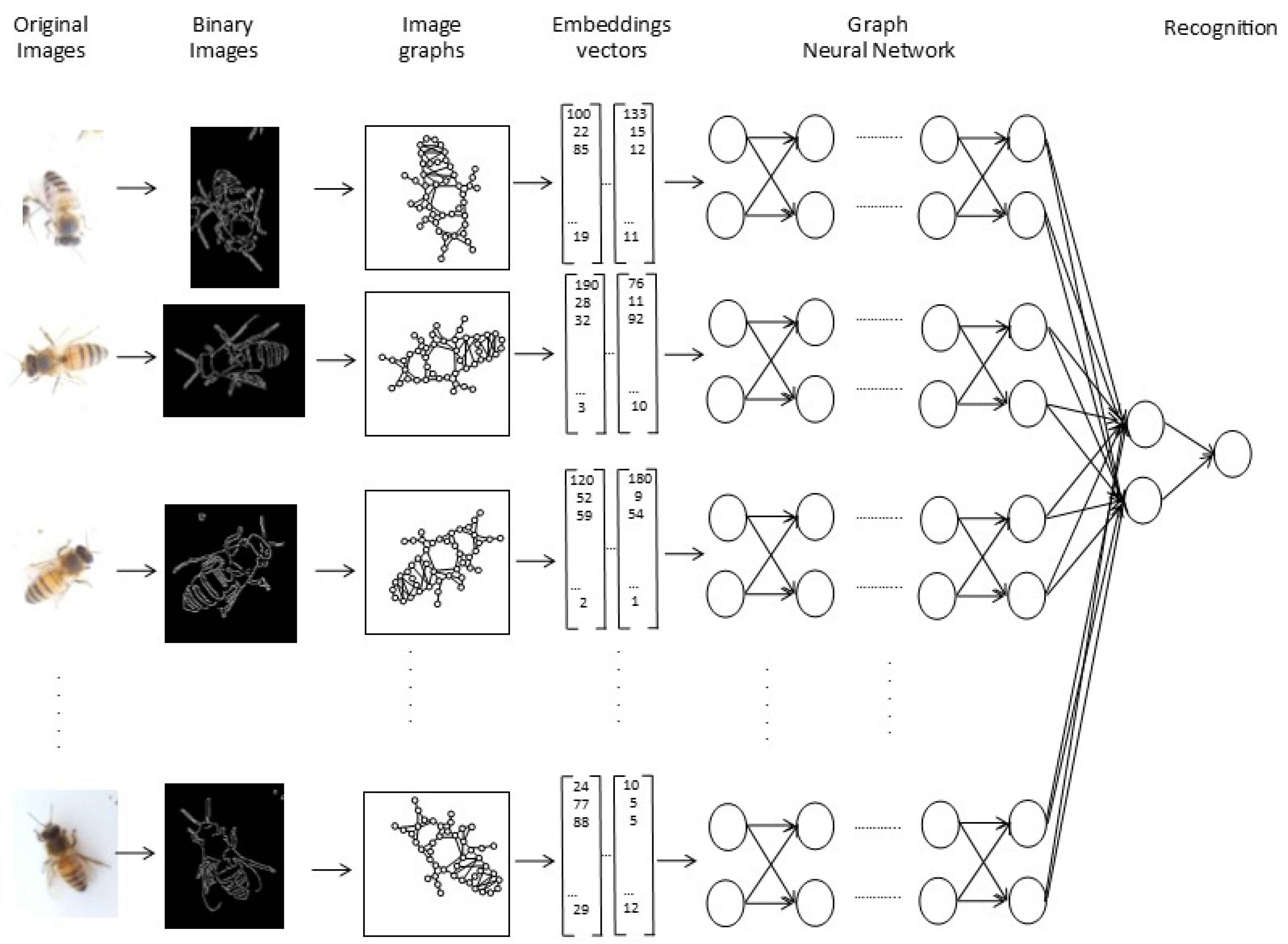
This work describes the implementation of an automatic recognition system that acquires real images of test apiaries during the four seasons of the year, with image-acquisition equipment using the Internet of Things at the entrance of the hive; the images are sent through a telecommunications system to be processed and analyzed in a server cluster. Finally, the bees are recognized in the images using DIP and GNN techniques, and a subsequent analysis of the abdomen of the Apis mellifera bee is carried out to detect the ectoparasitic Varroa.

This research paper is an extension of two previously published papers, namely Varroa Mite Detection in Honeybees Using Computer Vision [13] and Characterization of Honey Bee Anatomy for Recognition and Analysis Using Image Regions [34]. Both articles address the problem of the Varroa mite and describe the development of an automatic recognition system in apiaries. Based on these two studies, this manuscript describes new experiments conducted in other apiaries and hives.

This work is organized as follows: Section 2 describes a set of works related to the development of research using automated visual analysis methods in bee colonies; for a better understanding of the sections of this work, Section 3 defines some basic terms; Section 4 presents the problem statement of this research; Section 5 describes the materials and method used in this research and the complexity of developing automated visual-inspection systems in real environments; Section 6 explains the experiments carried out in different apiaries; limitations of the research are mentioned in Section 7; Section 8 and Section 9 present the conclusions and future work, respectively; finally, the proposed discussions are in Section 10.

2. Related Works

This section describes a set of works related to the development of research using automated visual analysis methods in bee colonies and Graph Neural Networks (GNNs) for image recognition. Only works related to the use of datasets with images and videos are highlighted, since the research focuses on the construction of an automatic recognition system. The methodology used, the software tools, and the results obtained in each work referenced in this section are compared. The objective of this comparison is not to highlight the limitations of the works, since they are structurally different; our objective is to show that in our country, we also work on the preservation and care of endangered species, such as the honeybee. Likewise, the references in this section have contributed to the development of this research, with references to the way in which image analysis techniques and object recognition in images are applied, their implementation in real environments, and the adaptations made to hives for the operation of the devices that constitute the automatic recognition system (ARS).

2.1. Works Related to Automated Visual Analysis Methods

In [14], results of bee detection and bee arrivals and departures in the hive are shown; the results show high levels of recognition, although the structure of the system is perceived as an invasive system in the hive, due to the stress generated. This system provides a practical solution to video surveillance in apiaries. The system consists of a device placed at the entrance of the hive consisting of up to 32 bidirectional tunnels the size of bees; this device uses a digital dash camera to acquire 640 × 480 color video frames at 30 frames per second, and from the video, it detects bees and tracks their movement through a sequence of frames; the system considers bee flight activity, along with knowledge of local conditions and behavior to indicate to beekeepers whether inspection or manual intervention in the hive is warranted; the system modeled frame-by-frame changes in bee position and orientation using Gaussian distributions; based on the results, they created a dataset of bee videos to train motion models and evaluate the systems; the system detected bees with an accuracy of 0.94; the system detected arrivals in 2% and accounted for departures in 7% of the dataset recorded.

Another work that measures the work done by bees is described in [15]; this system is a computational hardware platform together with a communication module; this work does not have a focus on parasite detection in honeybees, it only detects pollen carried to the hive, but it presents a training dataset useful for training a mixture of Gaussians. This system detects pollen-carrying bees by means of video surveillance at the hive entrance; the proposed algorithm creates a training dataset with previously detected bee images; MOG is applied to a set of training video frames; each training image is manually verified to ascertain whether or not it contains a bee with pollen; using the k-means algorithm, the pixels of each image of a bee without pollen load are grouped into two groups in the color space: blue background and bees; the centroid of both groups is calculated on all images of bees without pollen load; the mean centroid values are used in the Nearest Mean Classifier (NMC) to color bee segments in training and testing; the detection of pollen carried by bees is considered the previous step to pollination.

Regarding research works that have presented video surveillance systems focused on the detection of parasites, they are highlighted in the following paragraphs. In [8], a noninvasive system is described; in this work, real-time video processing is carried out that requires high processing times, which causes the need for high-speed devices with very high economic prices. The work describes an approach to detect Varroa mites in honeybees using foreground detection in video frames and a system applicable to other types of parasites that attack the honey bee; the videos are acquired by a camera system when the bees enter or leave the hive; the acquired videos are used as input for frame-by-frame processing using two steps: in the first step, the foreground is detected, and in the second step, the foreground is separated from the background in each video frame, then image fragments containing individual bees are extracted. The authors obtained different image classification results with different combinations of color models and feature-extraction methods; the authors report a maximum accuracy of 0.65 and a flight measurement of over 80%.

Another technological solution is present in [9] for the detection of the Varroa mite; the system presented here shows an overall accuracy in the detection of bees and Varroa mites close to 70%; but the system is invasive, which causes stress in the hive and is not reliable because honeybees cancel out any foreign agent placed inside the nest with wax. This research work uses cameras installed inside the hive; the camera incorporates an image-processing motion logic and uses a pre-trained CNN (Convolutional Neural Network) model to detect bees. The system collects objects to be detected; if the image does not contain objects to be detected, then it classifies the entire content of the image, and when locating multiple objects, a detection process is built that provides output bounding boxes or masked areas of the detected objects; the system consists of an end-node device, cloud service, and a central device for the online system as well as a mobile-phone application.

In [19], a noninvasive system is presented, with necessary functionality for its operation in an apiary. Although no details of the total economic cost are given, the system shows the implementation of the software with 5G technology; this technology would be difficult to reproduce in apiaries due to the distances that must be established between the passage of people and animals within the apiary. This system, called Var-Gor, monitors the infestation of the Varroa mite, installed at the entrance of the hive; Var-Gor is a device consisting of bee passage tunnels (width 25 mm, height 15 mm, depth 50 mm) with an autofocus detection camera combined with interface (process sensor: IV-HG10) and image capture equipment; the images obtained by the autofocus camera are combined with a developed template filter, classified by color and segmented. A template-matching algorithm is used to detect the elliptical and brown shape of the Varroa mite. For the bee, it uses a template-matching filter based on the relatively unique shape of the bee; a threshold of at least 75% similarity to the bee-shape algorithm is created for each captured image to ensure that the template-matching step is successful and to reduce the chance of obtaining erroneous results; Var-Gor was trained with 60% bees containing Varroa mites (Apis mellifera L.) and 40% not containing them. The authors report a shape-matching range with normal bees and Varroa mites of 70%; the system is equipped with sustainable and eco-friendly solar panels and batteries placed near the hives; it features a Wi-Fi-like network connection and easy-to-use mobile application software to alert beekeepers early in the case of Varroa infestation; Var-Gor features cloud storage and 5G smart technology.

In [20], an object-detector-based method for detecting the Varroa destructor mite in honeybees, using the YOLO and SSD object detectors together with the Deep SVDD anomaly detector, is presented; YOLO is a free piece of image-recognition software, which has been developed by the community to constantly improve the model. Its adaptation to the problem to be solved requires special configurations; for our work, adapting the software is not considered appropriate because it does not fit the research needs. The described system defines a dataset with six classes of images, of which it uses three: the first class is bees and the Varroa mite, the second class is healthy bees and infected bees, and the third class is data annotated only with the Varroa mite. The dataset was manually annotated with the LabelImg tool and the statistics are shown in different tables to be analyzed with a professional beekeeper; a neural network is trained by data augmentation using the Python library Im-gAug, and a wide range of various methods is applied to augment the image and create slightly modified derivatives of the original training data, without modifying the information contained in the images. In this way, the given task is solved for perfect-looking training data as well as for distorted, noise-added, or color-shifted images; the authors report a score of up to 0.874 in detecting infected bees and up to 0.714 in detecting the Varroa mite.

In [21], a computer-vision system is described for monitoring the level of infestation of the Varroa destructor mite in a hive by recording a video sequence of live Apis mellifera bees; this work presents lower recognition percentages compared to other research, and describes in more detail the levels of image processing; the video sequences of live Apis mellifera bees are in real environments, allowing the utility of the system to be adjusted to applications in real apiaries. The system can be described as follows: a video monitoring unit with multispectral lighting and a camera placed in front of the hive allows data to be acquired for a computer-vision algorithm based on deep-learning analysis of the video stream to count the number of bees and find the position of the identified Varroa mites; the computer-vision algorithm works at various processing levels: image acquisition, low-, intermediate-, and high-level processing. Each level executes other phases during processing to obtain the result. Image acquisition is designed for real-time image acquisition and compression; low-level processing is for raw image preprocessing and temporal image matching; at the intermediate level, the following phases are executed: low-level processing, background subtraction and segmentation, bee detection, Varroa identification, and localization using a Convolutional Neural Network; finally, in high-level processing, bee tracking and counting and infestation level estimation are executed. Based on a video sequence with 1775 bees and 98 visual mites, the authors reported that the algorithm measured an infestation level of 5.80% versus a real value of 5.52%.

In [22], a deep-learning approach is proposed to locate and count Varroa mites using images of the sticky boards taken by smartphone cameras. The method proposed in this research work combines hyperparameters and some image-enhancement techniques; the system achieves an average mean precision (mAP) metric of 0.9073 on the validation set. Although the metric (mAP) is high enough, the dataset proposed by the authors is composed of a limited number of images; a dataset update process, i.e., gradually increasing the dataset so that the system recognizes more images that could fit in the dataset, is not contemplated. The proposed system is described as follows: a dataset with 64 images of dimensions 8064 × 6048 pixels (48 Mpx) taken under different lighting conditions is built; the proposed approach is composed of several successive steps; first, the input images are preprocessed to improve their quality, specifically by motion blurring using conditional adversarial networks. Then, each input image is split (for training and inference) into smaller sections (or tiles). After that, a deep-learning model is trained based on the Faster R-CNN architecture to perform Varroa mite detection, and finally, automatic refinement is performed of the predicted bounding boxes after inference.

Other studies have also described the problem of parasites in bees; in [17], examples of surveillance systems that help to increase knowledge of the health of honeybees are described; video surveillance of honeybees is considered to be a tool to understand and improve bee health, identify risk factors associated with colony morbidity and mortality, disease prevention, and mitigation and early detection of threats, and discovery and characterization of new diseases and potential pathogens, including virulence and distribution. The results of this study propose the need for surveillance systems with designs that guarantee the collection of representative data, coordinate efforts, and standardize approaches.

2.2. Works Related to Graph Neural Networks for Image Recognition

In recent years, graphs have emerged as a topological representation for image analysis and processing; many powerful methods in image processing have been formulated on graphs, i.e., the vertex set in a graph is the pixels set in an image, and the edge set is determined by an adjacency relationship among the image [35]. In domains, data are commonly represented as graphs; graphs can model both the entities and the relationships between them; typically, the vertices of a graph correspond to some entities, and the edges model how these entities interact with each other [36].

According to the literature, many research works use graphs for automatic recognition, such as those referenced in this section. In [33], there are three steps to convert an image to a graph, which are explained below, according to the proposed model.

• Find graph structure. For the task involving the representation of an image, graphs are implicit; an image is highly representable by a type of graph; this type of graph is found in the next step.
• Specify graph type and scale. In the case of images, directed graphs are the most natural way to represent an image; through this type of graph, the vertices represent the positions of the matrix, and the edges represent the connectivity that exists between the pixels (positions).
• Design loss function. For the type of images used in this research, the graph classification task has been used; in this way, the model learns the representation of the graphs, and a supervised setting is used that provides labeled data for training.

Graph Neural Networks (GNN) provide a unified view of the images used as inputs in computer vision, which can be interpreted as special cases of a single, general data structure: GNNs can handle unstructured non-Euclidean data, a property that makes them valuable in problem domains where graph data are abundant [37]. Image recognition using Graph Neural Networks is a very extensive current area of research; in this section, some research works used as a reference for this research are described.

In [32], a method is proposed for detecting and classifying floorplan images using Graph Neural Networks; the method converts region-adjacency graphs (RAG) where each node is attributed using Zernike moments that correspond to a region in the original image; each edge of the graph is characterized using the distance between the centers of gravity of the connected components. In this way, the edges indicate an adjacency relationship between two regions encoded by incident nodes; the graphs are fed to a neural network, which classifies the nodes of the graphs using their attributes and topology.

In [30], a family of novel Graph Neural Network models is proposed that exploit edge features by finding that these features are not fully incorporated into graph convolutional networks (GCNs) and graph attention networks (GATs), including those of undirected or multidimensional edges; this proposed architecture filters node features while adapting edge features across layers, using deep learning.

A method for image classification using a Graph Neural Network model is proposed in [29]; the method converts the image into a region-adjacency graph (RAG) composed of superpixels as nodes, uses the graph convolution operator, and combines the residual and concatenated structure to construct a GNN which improves the feature-extraction ability; a loss function combining the additive angular margin loss function and the cross-entropy loss function is proposed, which increases the distance between classes and the compactness within classes for supervised learning.

A method for extracting vectorized roof lines and building roof structures from very high-resolution remote-sensing images is presented in [31]; the roof structure Graph Neural Network method consists of two components: (1) a multi-task learning module for extracting and comparing geometric primitives and (2) a relational reasoning module based on a Graph Neural Network to reconstruct the roof line structure.

As previous works show, there have been several efforts to develop an automatic inspection system in apiaries to alleviate the adverse effects of the Varroa mite. There are still problems to be solved in the systems described; some of the limitations of the methodologies described are the development of systems with tests in controlled environments, some with limited datasets, and invasive systems in the hive, which are expensive and use of open-source software that must be appropriate to the study in question.

For the technological system presented in this work, the development of a real-time, noninvasive system in the hive is presented with inexpensive, fast and efficient devices, with self-created software systems and four datasets that grow indefinitely as the images of the test apiaries are acquired; the above presents a low-cost technological development that can be applied in real apiaries.

3. Basic Terminology

For a better understanding of the following sections of this work, some basic terms are defined, which have been grouped into a set of subsections. The definitions are sorted according to the order of their use in sections.

3.1. Digital Image Processing

Image. Image I is a spatial representation of an object, a two-dimensional or three-dimensional scene [38]; this can be modeled by a continuous function of two variables $f(x,y)$ where $(x,y)$ are coordinates in a plane [39]. Every processed image is identified by an integer of the form: $I_1,I_2,\dots ,I_n$

Region. Region R of image I is a connected subset of a $2^n\times 2n$ array, which is made up of unit-square “pixels” [4]. A set of regions is represented by $R_1,R_2,\dots ,R_n$, and a region $R_n$ of an image $I_n$ is represented by $I_n{R}_n$; a set of regions of an image n is represented by $I_n{R}_1,2,\dots ,n$. In this work, we assume that the regions extracted from an image are contiguous and that regions can be represented by embeddings.

Segmented Image. According to [39], we represent a segmented image n as $S_b^c$ that consists of m disjoint regions $R_i$, as in Equation (1). The image I consists of objects and a background

$$S_b^c=\bigcup _{I=1,i\ne b}^m{R}_i,$$

(1)

where $S^c$ is the fixed complement, $R_b$ is considered background, and other regions are considered objects.

Vector. Vector V is a data structure that allows you to store a set of data of the same type, for example $1\times n$; it is used to store the results of images processed.

Matrix. Matrix M is an array with rows and columns, of a user-defined size, for example $n\times m$, and is used to store the image I; a matrix is considered to be a sequence of objects of the same type occupying a contiguous area of memory.

3.2. Graphs

Graph. Graph G is a pair $(N,E)$, where N is the set of nodes and E is the set of edges [27,40,41]. In the literature, the terms node and vertex are used; for the sake of simplicity in this work, we use both terms to refer to the graph.

Subgraph. The subgraph of a graph G is a graph, each of whose vertices belongs to $N\left(G\right)$ and each of whose edges belongs to $E\left(G\right)$.

Set of subgraph. The set of the subgraph from the graph G is represented by [42],

$$S{G}_1,S{G}_2,\dots ,S{G}_n$$

(2)

Such that for all, $k\in 1,2,\dots n,{\forall }_{i,j}$ and $i\ne j{v}_i,v_j\in S{G}_k$ with walks between $v_i$ and v_j. Every subgraph comprises a collection of vertices with strong affinities among them and can represent a region R of an image I.

Features. Quantifiable attributes, which in the graph domain are used to characterize vertices and edges. They are represented by numeric vectors such as: $V_i^F$ and $e_{ij}$.

Embeddings. Representations of compressed graph features, contained in a vector. For this research, embeddings are represented as: ${\vartheta }_i^F,{\epsilon }_{ij}^F,N_j^F,\gamma$.

4. Justification of the Research

The research proposed in this work is justified by the following:

• Develop a prototype based on hardware and software that carries out automated video surveillance of hives and emits an analysis of the images received from the apiary.
• The Varroa mite is a parasite that has a negative impact on beekeeping operations, which justifies developing a technological solution to the Varroa mite attack.
• Carry out video surveillance in apiaries with IoT technology and artificial intelligence methods.
• Observe the behavior of the honeybee in the hive.

5. Problem Statement

Varroa mites are invasive parasites capable of destroying entire colonies of honeybees if they are not detected in time; advances in image-recognition technology, miniaturization of computing devices, and research work in this area [8,9,13,14,15,16,17,19,20,21,22] have shown possible solutions to the Varroa mite problem; therefore, a research project with the design and implementation of a computer system is carried out to acquire images with IoT devices of the hives installed in the test apiaries, send the images through a wireless network and detect the presence or absence of the honeybee in the beehive through the use of digital image processing, generate graphs for the segmentation and representation of the images, and finally make use of Graph Neural Networks for recognition and analysis [29,30,31,32,37] of the thorax of the bees in image.

Formalism of the Problem Statement

Formally, given an image I modeled by $f(x,y)$, represented in a matrix M of $n\times m$ size that is broken down into R regions represented by $R_1,R_2,\dots ,R_n$, which features $V_i^F$ and $e_{ij}$ are generated and translated into a graph G with N nodes and E edges, then ${\vartheta }_i^F,{\epsilon }_{ij}^F,N_j^F,\gamma$ embeddings can be generated and stored in vectors that represent the input to a neural network for recognition and analysis.

Therefore, based on the above, we define the following propositions:

• $P_1$. Proposition 1: Conduct a binomial experiment to determine whether or not a bee exists at the entrance to the hive.
• $P_2$. Proposition 2: If $P_1$ is true, determine whether or not the detected object (bee) is a carrier of the Varroa mite.
• $P_3$. Proposition 3: Only if $P_1$ and $P_2$ are true is $P_3$ true, and an alert is issued.

6. Materials and Methods

This section has been divided into two subsections: the materials used and the method applied in the research. The materials used correspond to the hardware used in the construction of the prototype, and the method is the stages implemented in the software. Both sections are explained in detail in the following paragraphs.

6.1. Materials Used

In this section, the materials have been divided into four main systems, according to their application in the research, namely the apiary system, electrical power supply system, communication system, and software system. First, systems are listed together with a basic definition, and then in each paragraph, each of these is defined, together with each of its devices.

• Apiary system. This is the test apiary and the hive prototypes manufactured by the authors (within the educational institution where the research is conducted), with IoT devices and solar energy. Manufactured hive prototypes are installed in the test apiary and, for the purposes of this work, are called suitable beehives.
• Electric power supply system. This system consists of a solar electricity system. This solar electricity system is for the suitable beehive, which is installed in the apiary test. Network devices are connected to the normal electrical system. The name of the manufacturer, city, and country from where the equipment was sourced are described in paragraphs below.
• Communication system. This is the system for communication between the apiary, data-processing center (DPC), and the end user.
• Software system. This is the system of software created using open-source tools and operating in the DPC.

The four systems constitute the automatic recognition system, which operates in real time in uncontrolled environments. As specified in the previous paragraphs, the following subsections explain the characteristics (parameters) each device uses, for a better understanding of how each of them is applied.

6.1.1. Apiary System

The apiary system consists of test apiaries where the tests of the research are achieved, and a suitable beehive with the environmental requirements to be used with live honeybees; each beehive is identified by the registry provided by the Government Office of Agriculture.

The test apiaries are the spaces where a set of hives is located; from this set of hives, one or two hives were selected for the tests. Apiaries were selected with two main characteristics: first, they were located at distances that did not affect the transit of people, and second, there should not be any domestic animals near the apiaries.

The suitable beehive contains a set of special devices that allow for data and image acquisition; these devices are placed on the top of and the entrance to the beehive. The following paragraph lists the devices, functionality, and technical aspects.

• Two solar panels placed on the top of the hive, built crosswise for the acquisition of solar energy which feeds the Arduino devices, Raspberry Pi (Sony UK Technology Centre, Wales, UK), video camera and humidity, and temperature sensors. Technical information: Smart Projects, Ivrea, Italy 50 W, 12 Vdc, Polycrystalline, 36 Grade A Cells connected to a regular and an inverter; a deep-cycle battery acts as an energy-charging center (Epcom power line solar module-5012 of Changzhou City).
• A Raspberry Pi board, for sending and receiving information between the apiary and the DPC. Technical information: Raspberry Pi 4 Computer Model B Version 8 GB RAM (Sony UK Technology Centre, Wales, UK).
• A video camera for the acquisition of images in the hive entrance. The video camera is located at the top of the beehive entrance, with a direct focus towards the access, which allows the acquisition of images of individual bees and not in groups. (Technical information: Raspberry Pi High-Quality Camera 12.3 MP 7.9 mm diagonal image size.)
• An Arduino UNO to connect the humidity and temperature sensors of the hive. (Technical information: Arduino UNO microcontroller board. Technical information: Smart Projects, Ivrea, Italy, based on the ATmega328P. Humidity sensor DHT11. Temperature sensor LM35.)
• A wireless antenna to communicate the hive with the communication antenna router.

The general scheme of the suitable beehive is shown in Figure 1 and Figure 2. They show the real suitable beehive in operation inside the apiary. The system works 12 h a day to transmit information to the DPC. For the tests, 10 bee racks were installed inside the beehive with approximately 3000 bees, according to the beekeeper’s estimates.

6.1.2. Electrical Power Supply System

The electrical power supply system consists of two types of power: the power supply from the electrical network to enable functionality of the antennas installed in the apiary, and the solar energy system installed in the beehive. For the supply of electrical energy in the beehive, the system was designed as follows: two solar panels connected to a deep-cycle battery to guarantee the supply to the installed hardware. The energy consumption is 20 Watts per hour; the solar panels manage an energy of 120 Watts per hour for a cycle of 12 h, which guarantees devices will retain their full functionality. Figure 3 shows the power solar system operating in real time in the beehive.

6.1.3. Communication System

The communication system comprises point-to-point communication, which allows the DPC to communicate with the apiary permanently. The system works for a period of 12 h during the day; all data are collected in the “Liebre1” software agent system and are stored on high-speed devices for processing. The acquisition of data such as images, video, and hive parameters from the apiary to the DPC is performed every minute. Specifically, the automatic image-acquisition system (described below) sends images to the DPC for processing as shown in Figure 4. This system was installed exclusively to carry out this research project, so it is not used for the transmission of any other type of information.

6.1.4. Software System

The data-processing center (DPC) is constituted by a cluster of servers, where the received images are stored, processed, and analyzed with the software system.

The software system or software agent system was developed with the C programming language due to its proximity to assembly language; communication in the server cluster is carried out with the C Shell language of the Linux operating system, and the web system with HTML; Arduino programming is considered for the sensors connected to the beehive; to carry out the digital processing of the image, OpenCV [43] functions are used. With the mixture of these languages, the software agent system is responsible for processing the data and images collected from the hives. The stages of digital processing of the images received at the DPC, as well as the honeybee recognition and analysis for the detection of the Varroa mite in the image, are described in Section 6.2.

In addition to image acquisition, temperature and humidity parameters are collected and processed by the software system; these parameters are stored in a database, while the images are sent to a subdirectory on the host server. As the software system is in charge of performing video surveillance, a web page is provided for the beekeeper; this page displays the temperature and humidity data as well as the results of the analysis of the image extracted from the hive, i.e., whether the bee detected in the image is a carrier of Varroa mite or the bee is healthy.

In addition to the above, the software system also classifies the images for each monitored beehive; this classification is made because each beehive is identified by the registry provided by the Government Office of Agriculture, so when the image is transmitted from the test apiary, the identifier (ID) of each beehive is also transmitted, and in this way, it is possible to identify the origin of each image; this allows the monitoring of each beehive. Also, in the DPC, a preprocessing of the images is carried out to detect intrusions in the hive. This detection is made with image processing, which is explained in the paragraphs below.

6.1.5. Real Environments

In this subsection, reference is made to real environments because the research does not use synthetic data or controlled lighting environments, but instead uses data obtained from real-life situations. Thus, the factors that researchers face when developing automatic recognition systems are highlighted.

When computational systems are implemented for outdoor environments, different factors influence the images; several factors, such as lighting, real environment area, and object movement [15,23] must be considered. Lighting is directly related to environmental conditions. The area of the real environment where images are acquired for the analysis of objects is related to the movement of objects; if the objects being analyzed are living beings, the movement is unpredictable, since their positions cannot be controlled. Inanimate moving objects are usually moved by a device that regulates their speed. When living beings that have movement and different positions in the image are recognized, the distortions that must be treated in the processing are even more complex, and higher processing speeds are required [24].

For the above reasons, acquiring images in real time and scenarios has always been a challenge for digital image-processing algorithms due to weather conditions, problems caused by lighting, the location of objects, and even more so considering that the objects are living beings. In the following subsection, the proposed method is explained along with the methodology to deal with real environmental settings.

6.2. Proposed Method

The development of the method of this research is addressed using the flow chart in Figure 5; this diagram explains each of the phases of the method that constitute the algorithm for the recognition and analysis of Apis mellifera bees. Each part of the algorithm is explained in detail in the following paragraphs.

6.2.1. Automatic Image Acquisition (AIA)

Automatic image acquisition is carried out from the apiary test (the devices used for image acquisition are explained in Section 6.1.1); a video camera takes the image in the hive entrance with direct focus towards the access to allow images with individual bees, every minute, and transfer it to the Raspberry Pi with the Raspbian Operating System; this device is responsible for transmitting the image to the DPC. The transmission of images from the test apiary is carried out in 8-h shifts with a frequency of 2 or 3 times per week.

The test apiary is located at distances that do not affect the traffic of people or domestic animals.

Table 1. Real images obtained from the beehive entrance. Subfigures of letter (a) to letter (f) are examples of real images acquired from the test apiaries, with different illuminations in the Beehive Entrance.

(a)	(b)	(c)
(d)	(e)	(f)

shows examples of images obtained from the test apiary; as explained above, due to the position and focus of the video camera at the top of the beehive entrance, it is possible to acquire images with individual bees and not in groups. The characteristics of the images acquired in real time are disk size 304 KB (311,296 bytes), 1280 × 720 pixels.

6.2.2. Digital Image Processing (DIP)

Once the images are received at the DPC, they are processed using digital image-processing techniques. Although the examples show very sharp images (for the better understanding of the reader), the techniques were tested with different images of the possible positions of the bees in the entrance of the beehive, as well as considering the lighting on sunny days and cloudy days. Rainy weather is not considered, as bees do not outside of the beehive under such conditions.

Considering the research work [25,44,45], the applied DIP techniques are listed below, and each of them is described.

(a)

Cropping the image. This process segments the image into a fixed number of partitions; the camera focus allows the obtaining of individual bees by cropping the image;

Table 2. Example of cropping of image (a) in Table 1. Subfigures from letter (a) to letter (f) are the six partitions in which the image is divided after cropping.

(a)	(b)	(c)
(d)	(e)	(f)

shows the cropping procedure that was applied to the image of item (a) in Table 1. In this case, six segments of the original image are obtained, from item (a) to item (f). To each image segment, the following steps from (b) to (f) are applied; each step is briefly explained in the points listed below, and then, using the obtained partition, the TDI process is applied.

(b)

Applying the RGB2GRAY filter. The RGB2GRAY function is used to convert an RGB image to grayscale and remove hue and saturation information, and preserve lightness. The result of applying this function can be seen in

Table 3. Techniques of digital image processing applied to the image. Subfigures (a) show the original image after cropping, (b) is the RGB2GRAY filter, (c) is Gaussian Blur filter, (d) is Canny Edge filter and (e) find contours and draw contours of the original image.

(a)	(b)	(c)
(d)	(e)

with item (a).

(c)

Applying the Gaussian Blur filter. This low-pass filter is applied to reduce the value of the irregularity and smoothness pixels in the image. The result of applying this filter can be seen in Table 3 image with item (b).

(d)

Applying the Canny Edge filter. This filter is used to detect all edges existing in the image by obtaining the gradient, non-maximum suppression, and threshold hysteresis. The result of applying this filter can be seen in Table 3 in item (c).

(e)

Find contours. This processing allows the discovery of the external and internal contours of a binary image. The result of applying this function can be seen in Table 3 in item (d).

(f)

Draw the contours. This procedure is used to highlight the contours obtained in the previous step. The result of applying this function can be seen in Table 3 in item (e).

For a better understanding of the application of DIP phases, Table 3 shows the changes in the image. Starting with the original image, after having performed the crop, the following images (from left to right) are obtained after the RGB2GRAY filter, Gaussian Blur filter, Canny Edge filter, Find contours, and Draw contours, respectively.

6.2.3. Image Graph Generation

As we referenced in Section 2.2, the representation of the images with graphs is carried out in this research work; then, the representation of the image resulting from the DIP process is converted to a graph. The complete conversion process is explained in paragraphs below; the explanation is organized as follows: we explain the transfer of the binary image to a matrix; then, the procedure is explained in detail on how the image features are obtained and how the embedding vectors are obtained from the features; we specify the type of graph that is generated from the matrix and the scale; finally, we explain the validation of the obtained embeddings and the features of the graph.

First, once the image has been converted to a binary image and placed in a matrix of ones and zeros, a traversal procedure is performed from the top left of the matrix in a left-to-right direction, position by position of the matrix, until it has been traversed in its entirety; the objective of this search is to locate the positions of the matrix that contain a value of 1; positions with a value of 0 are ignored and will not form part of the graph that is built from the matrix; Figure 6 shows how the traversal procedure is performed.

When a value of 1 is located in the position of the matrix, the second step is executed (explained below). For reference purposes and for the sake of simplicity, positions with a value of 1 are called pixels in this work.

The second step is obtaining the features of the position of the matrix with value 1. Each time a value of one is found in a position of the array, a set of features is obtained and stored; features are quantifiable attributes that characterize a phenomenon under study [37]. In this research, the obtained features are of the pixel and the neighbors of the pixel, as we explain below; Figure (a) of

Table 4. Way and the direction in which the search for neighbors is performed (a,b).

(a)	(b)

shows how the pixel’s neighbors are visited, and Figure (b) of Table 4 shows the direction in which the search for features of the neighbors is performed for each of the positions of the matrix (when the value of the pixel is 1).

The set of features is listed below, and the way they are obtained is explained in the following paragraphs.

(a)

Position of the pixel in the matrix.

(b)

Locations of the neighbors using the Freeman chain code [13,46,47].

(c)

Pixel characterization.

(d)

Number of neighbors of the pixel that have a value of 1.

(e)

Weight of the pixel.

(f)

The pixel with value one is counted to obtain the total number of pixels with value one in the image.

First, after the position in the matrix is located as a pixel equal to 1, the position is saved in the format $(n\times m)$ (Matrix definition in Section 3.1). An example case of Figure 6, position of the matrix $(1\times 1)$, is considered.

For the location of the neighbors using the Freeman chain code, the 8 surrounding neighbors are checked clockwise from 0 to 7 (Figure (b) of Table 4) taking into consideration the search based on the Freeman chain code [46,47]; if a neighbor has a value 1, its position is considered to be features of the pixel or features of the central vertex, represented by $V_i^F$. For the example case in Figure 6, the positions of the neighbors 0, 1, 2, and 6 are considered as features of the pixel at position $(1\times 1)$; as we explained, only the neighbors with values of 1 are considered to characterize the pixel. Neighbors are considered to be the features of all the vertices of the neighborhood and represented as $e_{ij}^F$.

Then, for pixel characterization, we consider the next example, Figure 6, for the position $(1\times 1)$ of the matrix, neighbors 0, 1, 2, and 6 are considered to characterize the pixel; in this example, a pixel of the position $(1\times 1)$ of the matrix in an 8-bit binary representation is 11100010 and is considered a border line of the image. For now, 32 possible positions have been characterized out of the 64 existing combinations as follows: if the position combinations found are 11111111, then a central bit (central pixel) is located; for a combination 00000000, an isolated bit (pixel isolated) is found and is not considered; for the case of 00101000, a corner is located; in this way, each position with a bit on must be characterized and the third characteristic is obtained. Thus, at the end of the search for all pixels with value 1 in the binary matrix of the image, all pixels would be characterized. Pixels with similar features build neighborhoods; for this research, neighborhoods will build subgraphs (see Section 3.2 for subgraph definition) and represent distinct groups of vertices and edges, as specified in [37].

To obtain the number of neighbors of the pixel that have a value of 1, a count of these is performed; for the case of the matrix position, a total of 4 neighbors is obtained.

The weight of the pixel is assigned according to the number of bits on and the pixel’s characterization. For example, a bit with the corner characteristic has a weight of 10, which gives it a high importance; a pixel with the central pixel characteristic has a weight of 3, and its importance is not significant. The characteristic of the number of pixels in the image is obtained with a summation of all the positions with a value of 1 in the matrix. Once all the features in the array are found, they are stored as indicated in the third step.

In the third step, we build the scene graph for the image to be processed. At this point, we specify the graph type and the scale [33]: we deal with directed graphs where the edges of the graphs are all directed from one node to another to provide more information about the image; the nodes and edges of the graph have the same types, so we have homogeneous graphs; the input features vary over time so we have temporal information and, hence, dynamic graphs.

Then, according to the above, taking into account the search from Step 2, a node of the graph is built for each bit 1 (on), which is located; each node of the graph stores the features of the position in question; it is necessary to indicate that the features are stored with numerical values in each of the positions of the node. Each node is linked to the existing nodes in the graph according to its creation, which allows the graph to be created. Each link created must store the relationship that exists between nodes; for example, if a node is a corner and has a relationship with a central pixel, with another corner, and so on. In the case of the root node of the graph, if no node of the graph exists, then the first node created is considered the root of the graph. Once the image graph has been completely created, a traversal is performed, as indicated in the fourth step. A graphical form of this step can be seen in Figure 7.

In the fourth step, once the image graph has been created, as shown in Figure 7, and the features stored, a graph traversal is performed to obtain embeddings; embeddings are compressed feature representations that reduce feature vectors to build low-order models and make datasets linearly separable. The embeddings are stored in the feature vectors of the analyzed image and serve as input to the neural network. This step is executed as follows: 5 vectors are created with the size of the rows of the image, each node visited by depth-first search in the graph will provide the value of each of the five features stored in the node; then, at the end of the graph traversal, the 5-feature vectors are obtained.

In the fifth step, validation is carried out on the obtained data (embeddings) for the input to the neural network; in this step, a data-validation procedure is executed on the five obtained vectors. To perform the data validation, value thresholds are established for each of the six characteristics; if the values obtained in the search are not within the verified thresholds, the value is rejected, and a value of zero is inserted instead. This last step allows us to validate that the values sent to the neural network are valid and fall within a range of values.

In addition to the characteristics of the graph nodes obtained previously, an additional characteristic of the graph is also obtained: the density of the graph, as explained in the sixth step.

The sixth step obtains the features of the created graph. As a complement to the pixel features, a characteristic of the graph is obtained: the density of the graph. This characteristic is obtained by determining the number of vertices that the graph contains [27,40,41].

This concludes the image and graph procedures. The next subsection explains how the neural network model is used for image recognition from the created data structures.

6.2.4. Training and Test Dataset Construction

Graph Neural Networks have been recently applied to image classification tasks with different techniques in research works [28,29,30,31,36]; the next sections explain how GNNs are used in bee recognition after features are obtained and the graph is created. First, the training and test datasets are defined in this section. For better understanding, tables with images that are converted to graphs (this conversion was explained in Section 6.2.3) are provided. How embedding vectors are created and how vector embeddings are used in GNN is explained in the following sections.

Training and test dataset. The training dataset was constructed with the following types of images:

(a)

The beehive entrance showing different positions,

(b)

Bees infected with Varroa mite,

(c)

Bees in positions that are considered complex for recognition, and

(d)

Intruders that can appear in the beehive entrance.

Each training dataset is exemplified below with an image table. It is important to note that all images processed and used in this research are acquired from the test apiaries.

Table 5. Bees in the beehive entrance showing different positions.

shows images with bees in the beehive entrance showing different positions. Because bees in the beehive can appear in different positions, this table shows some of the positions in which bees have appeared in the images.

Table 6. Bees infected with the Varroa mite.

of images with bees infected with the Varroa mite. This table shows a subset of images (of the complete set) that have been considered for training the Graph Neural Network and achieving the recognition of infected bees.

Table 7. Bees in positions that are considered complex for recognition.

shows images with bees in positions that are considered complex for recognition. The images in this table exemplify only some of the positions that have been considered complex for recognition and subsequent analysis; the following section explains the results obtained with this type of image.

Table 8. Intruders that can appear in the beehive entrance.

shows images of intruders that can appear in the beehive entrance. Because the hive is exposed to the environment, intruders can appear in the beehive. This table shows a subset of intruders (of the complete set) that have been captured by cameras. During the recognition processes, these insects are not considered.

The test dataset was built from all the images obtained from the test apiaries; we can obtain many images from the test apiaries because the automated system runs daily, as explained in Section 6.2.1.

6.2.5. Graph Neural Network Training

The GNN is trained with all images shown in Table 5, Table 6, Table 7 and Table 8; the transductive learning method is used, so both the training and test datasets are exposed to the GNN. The GNN forward pass is performed in two processes: the input graph containing all the image features is converted into useful embeddings, and the classification task is executed; both processes are explained in paragraphs below.

The input graph containing all the image features is converted into useful embeddings. The GNN computes embeddings at each vertex in the input graph using a transition function Ϝ, which allows the computation of the next neighborhood representation from the current representation; as the neighborhood size is variable, the transition function is applied symmetrically.

An embedding for any vertex is dependent on:

(a)

The features of the central vertex, defined as ${\vartheta }_i^F$.

(b)

The features of all adjacent edges, defined as ${\epsilon }_{ij}^F$, if there are features of the adjacent edge.

(c)

The features of all vertices in the neighborhood, defined as $N_j^F$.

(d)

The embeddings of previous iterations of all vertices in the neighborhood, defined as $\gamma$.

The transition function Ϝ successively calculates the embeddings with the input variables and the output variables; for this, a maximum neighborhood size was established, so if a vertex has no existing neighborhoods, a null vector is created. Therefore, from the above, there are four feature vectors regardless of the vertex being considered, mathematically formulated as in [37], as follows:

$$h_i^k=\sum _{i=1}f({\vartheta }_i^F,{\epsilon }_{ij}^F,N_j^F,\gamma )$$

(3)

Ϝ is applied iteratively until a stable embedding is achieved for all vertices in the input graph.

Once the first iteration is performed, any vertex embedding encodes the neighborhood features within a range of just one edge. In the second iteration, any vertex embedding is an encoding of the neighborhood features within a range of two edges away and so on; in addition to the above, so that all vertices remain connected, the identity matrix $I_n$ is added to the normalized adjacency matrix A, which prevents unwanted embedding scaling from occurring.

The classification task is executed.

Once the previous steps are executed, the image classification process is carried out. The GNN performs the proposed classification in Section 6.2.4.

6.2.6. Calculation of the Downward Output

The cross-entropy loss function [29,33] in this work is used for labeled nodes in the training set. In this work, node-level tasks [26,27,33] are considered to perform node classification and clustering; node clustering allows nodes to be divided into several disjoint groups to be able to classify them; from a supervision perspective, we use a supervised setup with labeled data for training.

6.2.7. Graph Neural Network for Recognition

At this stage of the flowchart, the response of the neural network is captured; if the recognition response of a bee is positive, the image-verification process is also verified by the presence of the ectoparasite in the bee. If the response to the presence of the ectoparasite is positive, the user is informed; otherwise, another image is processed.

6.2.8. Phases of the GNN

As a conclusion to everything explained in the previous paragraphs and for better understanding, Figure 8 shows each of the phases of the project.

Original images. Original images are the set of images selected to train the Graph Neural Network. For simplicity, we have used four sets of images, which are, “bees in different positions for recognition”, “bees infected with the Varroa mite”, “bees in positions that are considered complex for recognition” and “intruders that can appear in the beehive entrance”; all these sets are built with real images obtained in the apiary, and generated with the software-cropping process carried out in C language.

Binary image. This is the image obtained after the TDI, from which the object characteristics are extracted; the noise may remain in this image, which is filtered by the generation of the graph.

Image Graphs. These are unique graphs generated from the binary image; the way in which the image graph is obtained is described in Section 6.2.3. A basic definition of this data structure and how it is constituted is described in Section 3.2.

Embedding Vectors. These are the representations of compressed characteristics that are associated with vertices, edges, and neighborhoods of the image represented in the graphs; this set of vectors store the features extracted from the graphs (according to the procedure explained in Section 6.2.5) and are used as input data to the neural network. This data structure is described in Section 3.1.

Graph Neural Network. The neural network receives the input vectors for processing and generating object recognition in the scene.

Recognition. All steps are capable of issuing an alert in the case of the following detections: the insect detected by the system is not a bee in the entrance (there is an intruder), the insect detected by the system is a healthy bee in the entrance, or the insect detected is an infected bee.

7. Experiments

This section presents the methodology to carry out the execution of the experiments; for this purpose, three subsections are presented. The three subsections are listed and explained in the following.

(a)

The first subsection defines a set of terms used in the experiments; these terms are placed in this section so that the reader has a better understanding of the experiments.

(b)

In the second subsection, the experiments performed are described. This subsection uses four sets of images (training dataset) presented in Section 6.2.4: the first dataset is “bees in different positions for recognition”, the second dataset is “bees infected with the Varroa mite”, the third dataset is “bees in positions that are considered complex for recognition”, and the fourth dataset is “intruders that may appear at the entrance of the hive”; all datasets of images are used for training the Graph Neural Network, which is trained with the procedures described in Section 6.2.5.

7.1. Terms Used

This subsection lists and defines a set of terms used in the process of describing the experiments performed.

Researcher. They are the people responsible for visually verifying the images and contrasting the results of the software system.

False positives. These are the results of the software system indicating the presence of a bee in the image, but, through verification by the researcher, such a bee does not exist. A false positive is also considered when the system detects the presence of a bee in the image, then the image is analyzed, and the presence of a Varroa mite is determined, but the parasite does not actually exist on the bee.

False negatives. These are the results of the software system not indicating the presence of a bee in the image, but, through verification by the researcher, the bee exists.

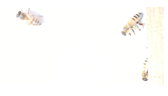
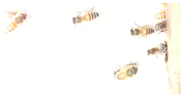
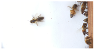
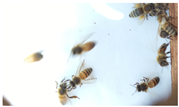
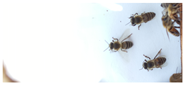
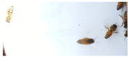
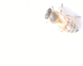
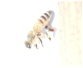
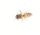
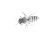
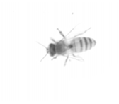
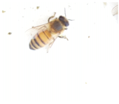
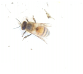
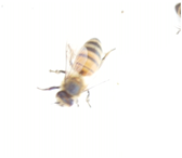
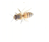
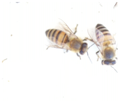
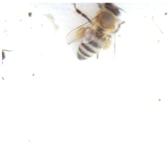
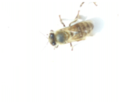
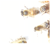
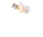
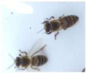
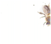
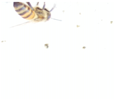
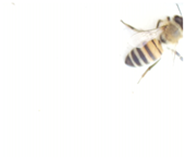
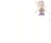
Images of Apis mellifera bees. Table 5 shows a set of images that show the bee at the beehive entrance. These images show some of the positions of the bees in the beehive.

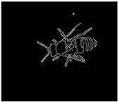
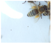
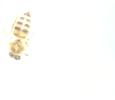
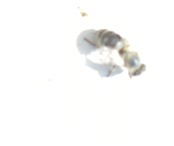
Images of Apis mellifera bees with the Varroa mite. Table 6 contains a set of images that show bees with the Varroa mite at the entrance to the beehive. These images show some of the positions of bees infected with the Varroa mite at the entrance to the beehive.

7.2. Experiments

The experiments were divided to measure two parameters: first, the speed with which the bee is recognized at the hive entrance, and second, the recognition accuracy of the evaluated techniques. The next two items in the list explain each parameter evaluated and some considerations.

(a)

The speed with which the bee is recognized at the entrance of the hive. With this experiment, we wanted to measure the time that each technique takes to recognize the bee at the entrance of the hive, because we are evaluating a real-time recognition system. For this experiment, object occlusion in the image is not considered because the camera placed at the entrance of the hive has the focus necessary for the acquisition of individual bees, in addition to the cropping process that is performed to segment the acquired images; this process is explained in detail in Section 6.1.1. The recognition speed is measured in milliseconds to allow the evaluation of the times of each technique.

(b)

The recognition accuracy of the evaluated techniques. With this measurement parameter, we wanted to evaluate the recognition accuracy of the object in the image, in order to determine the percentages of certainty of each evaluated technique.

With these two measurements, we can compare the speed and accuracy of each technique, considering that kNN is a fast classifier that needs few parameters in its execution with little processing time; in contrast, GNN is a recognition technique that requires more parameters and more processing time.

The following nine items are the list of experiments performed.

(a)

Section 7.2.1—Bee recognition at the beehive entrance experiment.

(b)

Section 7.2.2—False positives at the beehive entrance.

(c)

Section 7.2.3—False negatives at the beehive entrance.

(d)

Section 7.2.4—Recognition of bees with the ectoparasite Varroa.

(e)

Section 7.2.5—False positives in bees infected with the Varroa ectoparasite.

(f)

Section 7.2.6—Percentages of false negatives in bees infected with the Varroa ectoparasite.

(g)

Section 7.2.7—Recognition time of the bee at the beehive entrance and detection of Varroa mite.

(h)

Section 7.2.8—System times to recognize bees in the beehive entrance.

(i)

Section 7.2.9—Recognition of bees with different positions.

Experiments (a), (b), and (c) are performed with datasets containing healthy bees and bees infected with the Varroa mite; the recognition accuracy parameter is evaluated with the kNN technique and with the GNN technique. Results of both techniques are compared.

Experiments (d), (e), and (f) are performed with bees infected with the Varroa mite, and the two techniques, kNN and GNN, are evaluated, with the accuracy parameter. Both techniques are compared.

Once the accuracy parameter is evaluated, with both techniques, we evaluate the recognition speed parameter with experiments (g) and (h); i.e., we want to know which technique offers the best recognition times of the object in the image. The research question that remains here is whether we have a technique that offers us speed and accuracy at the same time when we have a real-time recognition system.

Finally, we experimented with the recognition of bees in different positions (see images in Table 7), experiment (i); the parameter evaluated with this experiment is recognition accuracy.

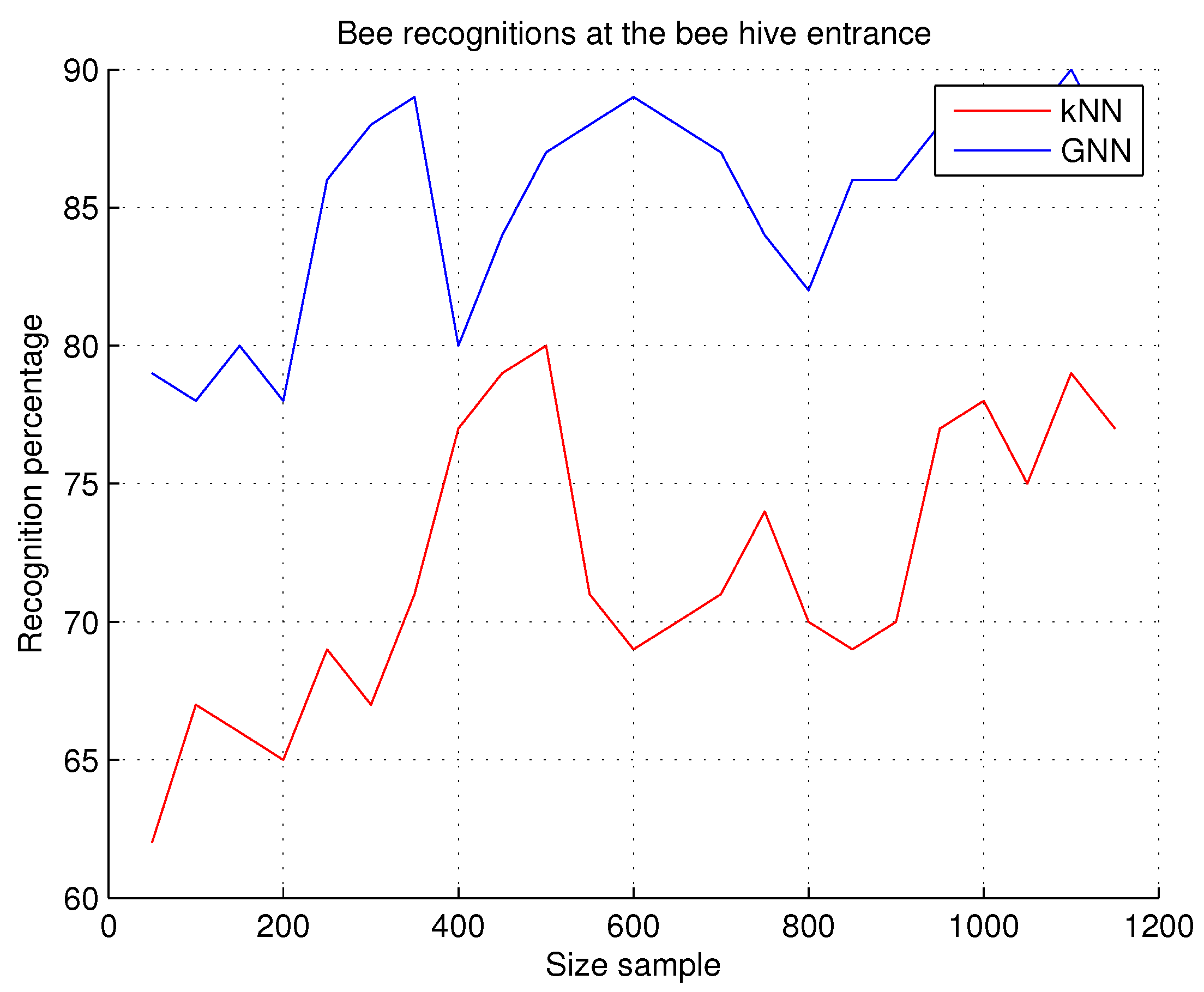
7.2.1. Bee Recognitions at the Beehive Entrance

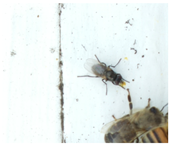
This experiment allows us to measure the accuracy of bee recognition in the beehive entrance, through the software system; the result is considered accurate when the software system outputs the bee recognition result at the beehive entrance, and this result is verified by the researcher. This experiment is performed every time an image is transmitted from the apiary to the DPC, and it is necessary to verify if the object in the image is a bee because other different insects, such as wasps, ants, or beetles may be contained in the image; see the table of images of intruders that may appear in the hive’s entrance. Sets of 50 images are incrementally considered to obtain the recognition percentage total, i.e., the result is obtained by dividing the number of times that the system accurately recognized the bee at the beehive entrance by the number of verified images. The number of images in each set is incremental, i.e., the previous set of verified images is considered; for example, the first 50 images are taken and the recognition percentage is obtained; then the first 50 images are considered again, 50 more images are added and result is obtained again, and so on.

Observations. GNN is a recognition technique that provides higher recognition rates if the sample size is increased. The recognition rates, as shown in Figure 9, reach almost 90%, but the processing time is higher. The image transmission time between the apiary and the data-processing center is 1 min, which facilitates the system response time; but now, if we process 100 images per minute, the system response time for each image is not acceptable. In the case of the kNN technique, although the recognition rates are lower, the recognition speed is acceptable. If we evaluate the precision with the speed, we obtain better recognition responses with GNN, but at the cost of high processing times. This can be verified in the experiment Section 7.2.7 explained below.

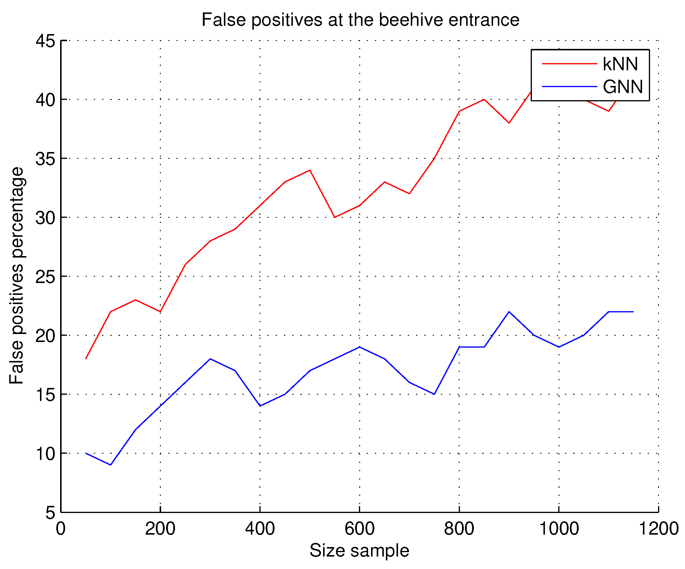
7.2.2. False Positives at the Beehive Entrance

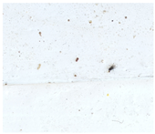
We consider a false positive when there is no bee in the image, but the system detects the bee, i.e., it recognizes the bee in the image, but without it existing. This experiment is carried out because the image acquisitions are in real environments and the presence of noise in the image is constant; the shapes generated by the segmentation algorithms can be similar to the shapes of the beehives and generate false positives; see Table 7.

Observations. Figure 10 shows a low percentage of false positives using the GNN technique, compared to the false positives shown using the kNN technique. During the experiments, a better performance is shown in images that do not contain bees using GNN. Therefore, the recognition accuracy is considered better when using GNN.

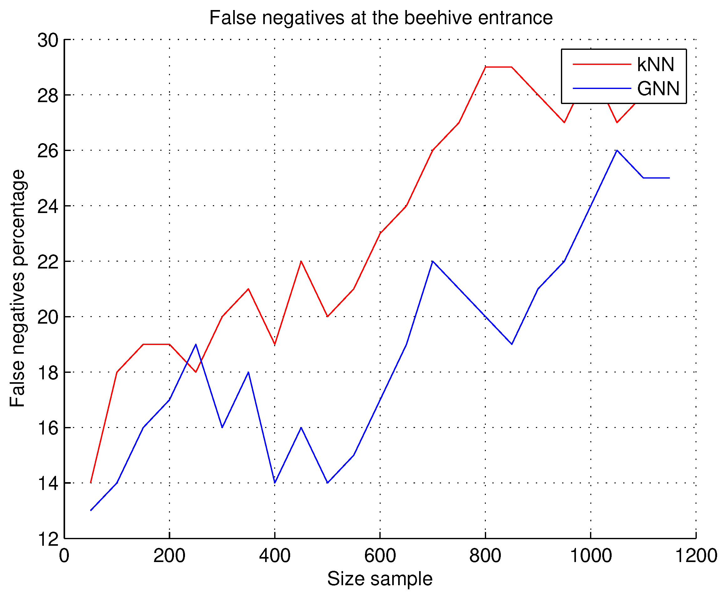
7.2.3. False Negatives at the Beehive Entrance

A false negative is when there is a bee in the image, but the system does not detect it, i.e., it does not recognize the bee that does exist in the image. Since the project uses images of real environments, the following situations may occur: the bees appear in different positions at the entrance of the hive, the images contain incomplete bees, and the images may contain different sizes of the bee in the image, due to the position of the camera in the hive; as a reference to this, Table 7 contains images with bees in positions that are considered complex for recognition.

Observations. The results obtained show a lower number of false negatives with the GNN technique, as can be seen in Figure 11, but it should be noted that the system response times are still longer with the use of this GNN technique. Lighting during image acquisition is an important factor to consider. The system gives better results on cloudy days because the shadow of the hive is not projected onto the hive entrance. In the case of rainy days, no experiments of any kind were carried out.

7.2.4. Recognition of Bees with the Ectoparasite Varroa

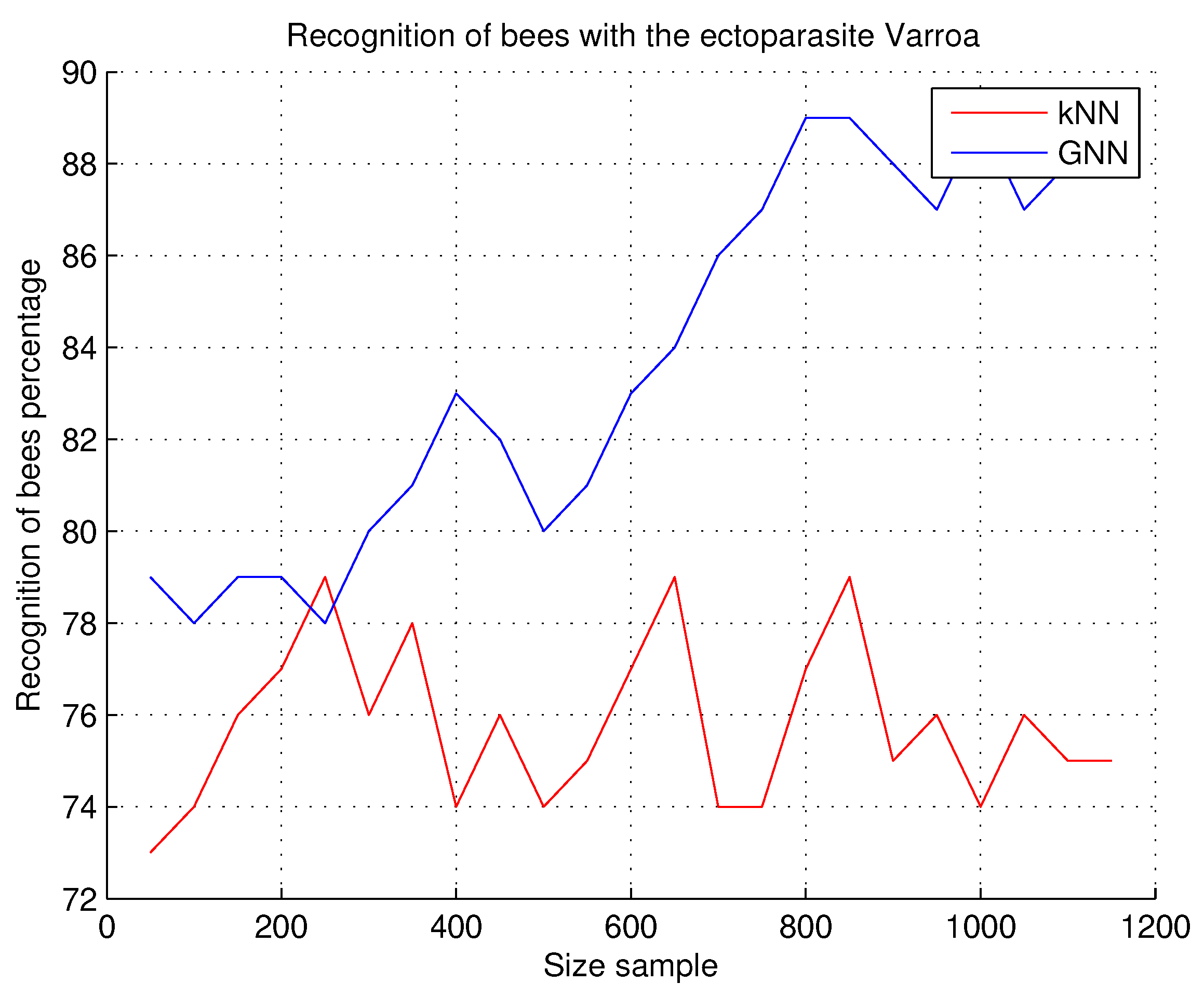
This experiment is the first of three experiments, in which the objective is to detect the presence of the ectoparasitic mite Varroa, after recognizing the bee at the entrance of the hive; the results obtained in this experiment do not consider false positives or false negatives, only the result of the execution of the system, i.e., if the bee recognized in the image is infected with the Varroa mite or is a healthy bee.

Observations. In this research work, we seek the precision in the recognition of the honeybee at the entrance of the hive and the precision in the detection of the Varroa parasite in the detected bee. Figure 12 shows the results of this experiment; a better precision with the GNN technique was obtained, but it was not very different from the kNN technique; kNN is a plane division technique that can be effective when the feature vectors are very well defined. For this study and experimentation, we consider that both techniques work correctly in real environments with very acceptable results.

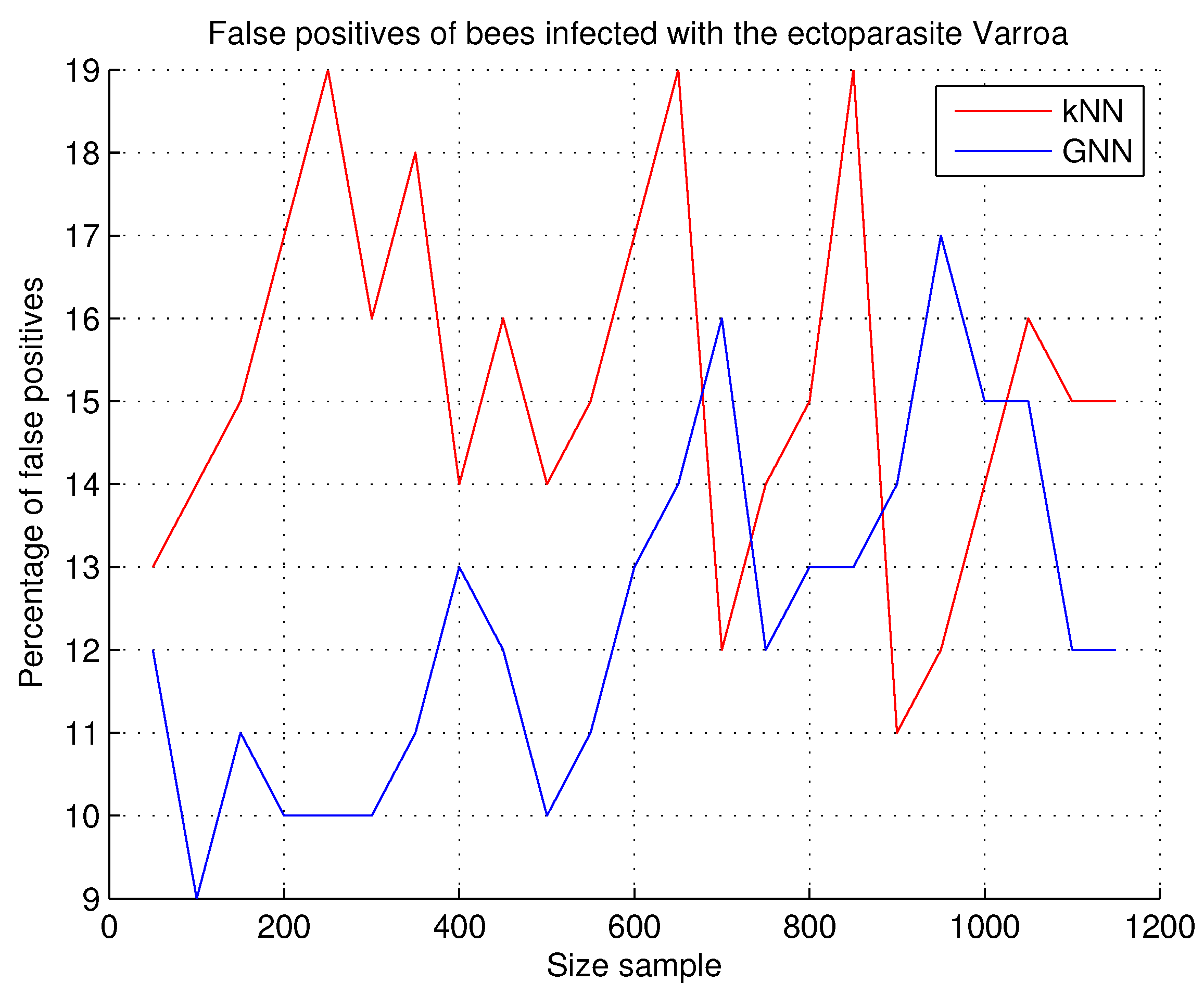
7.2.5. False Positives in Bees Infected with the Varroa Ectoparasite

A false positive is when there is no bee infected with the Varroa parasite in the image, but the system detects the bee infected with the parasite, i.e., a recognition of the infected bee in the image is issued, but it does not exist. This experiment was carried out with the support of the beekeeper in the following way: each time the system positively verifies a bee with a Varroa mite, the response and the image are issued to the researcher and the beekeeper to verify the obtained result; a false positive is indicated in the case that the response is incorrect.

Observations. The results of the experiment are shown in Figure 13. When the sample size is low, the results of both techniques are very dissimilar, but when the sample size increases in the number of images, the results tend to be equal; as the image shows, the results become better using the kNN technique when the sample size ranges between 800 and 1000 bees. An observation process was carried out with both techniques to verify the causes of these results; it was observed that the samples do not have enough variety to achieve the expected results. For this sample, it was necessary to increase the dataset to experiment with the number of images and to experiment with both techniques, and, in this way, be able to evaluate them.

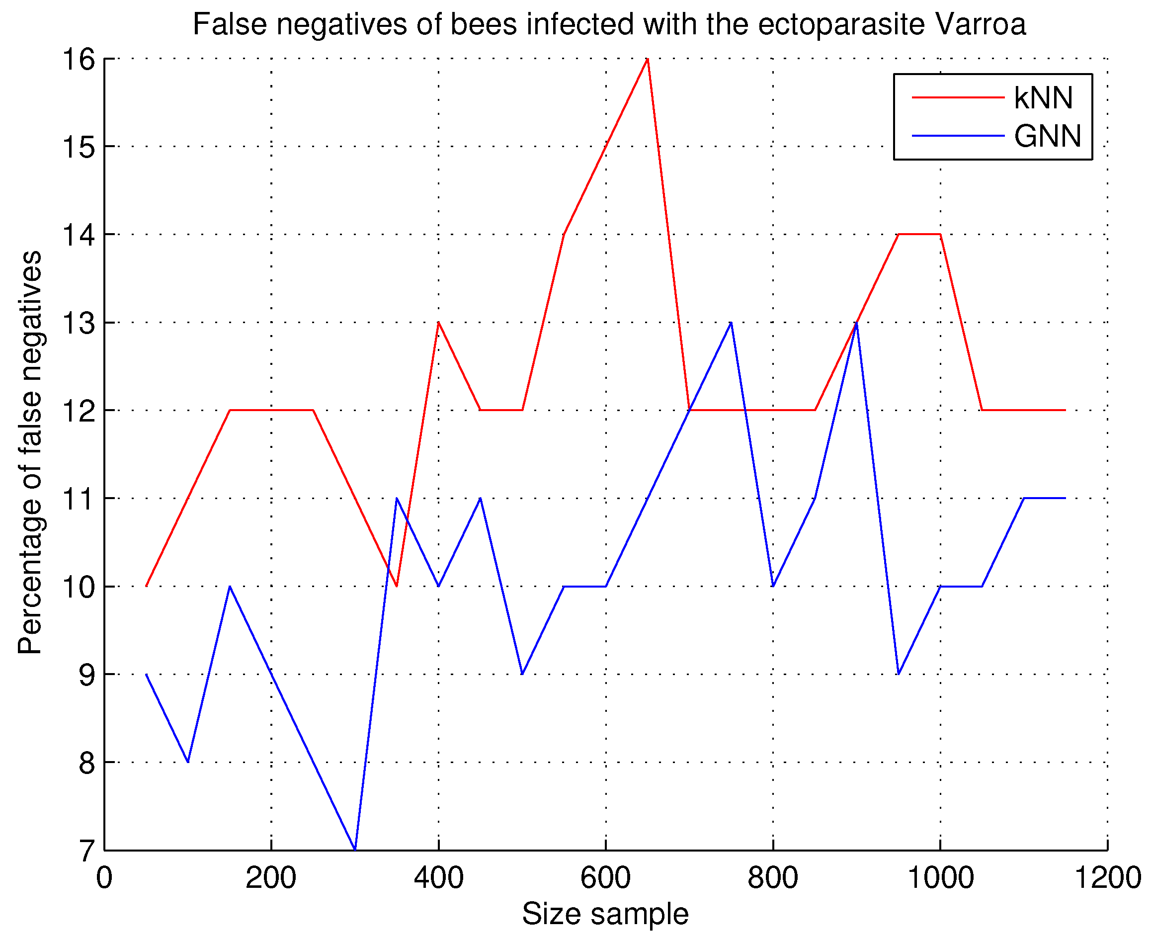
7.2.6. Percentages of False Negatives in Bees Infected with the Varroa Mite

This experiment is performed to determine the percentage of images that the system rejects or does not recognize as a bee infected with the Varroa mite, but if the image does contain the Varroa mite because it has already been verified by the researcher and by the beekeeper, i.e., the presence of the parasite in the bee is certain. For this experiment, the sets of images of the bees that present the Varroa mite are used; some examples of images from this dataset appear in Table 6; the evaluation percentages of this experiment can be seen in Figure 14.

Observations. According to the results obtained with the developed software system, we consider the false negatives obtained with both techniques to be within an acceptable range for this research. In Figure 14, the kNN technique showed better results for this experiment by obtaining a lower number of false positives; the classification performed with the kNN activation function is more accurate.

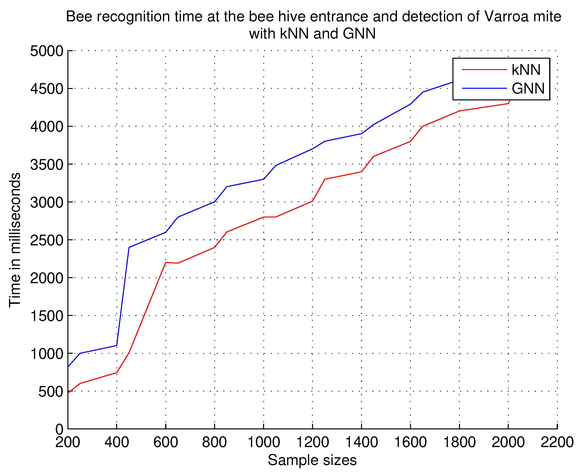
7.2.7. Recognition Time of Bees at the Beehive Entrance and Detection of the Varroa Mite

This experiment measures the time taken by the software system to recognize bees at the hive entrance and detect the Varroa mite; the experiment determines the amount of time needed by the system to generate the recognition result. False negatives and false positives are not considered in this experiment.

Observations. As shown in Figure 15, in this experiment we have found that the recognition time of bees at the hive entrance and the detection of the Varroa mite are lower with the kNN technique, but when considering false positives and false negatives, the best responses are obtained with the GNN technique. The above indicates that the kNN classification time is better, but lacks exact recognition; the results obtained with the GNN technique are more precise in classification, but have the highest time consumption per sample.

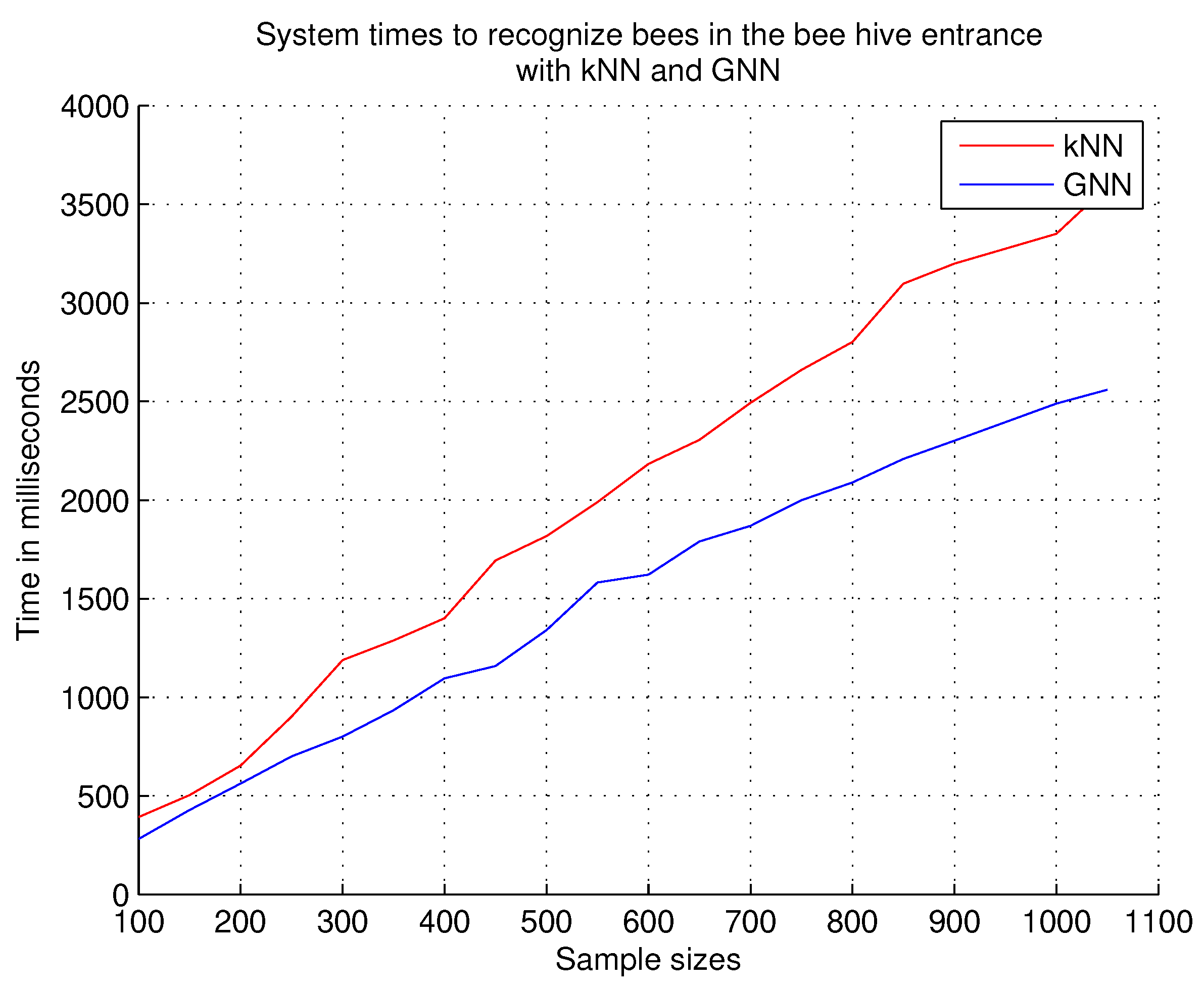
7.2.8. System Times to Recognize Bees in the Beehive Entrance

The objective of this experiment is to measure the time consumed by the system for the recognition of the bee at the entrance of the hive for each sample size presented to the system; for this experiment, the sample size starts at 100 images and incrementally up to 1100 images. In other research works, it is specified that the techniques that use graph structures are not suitable for real-time recognition, due to the time they consume; with this experiment, we demonstrate the opposite. In this experiment, we do not consider false negatives and false positives, i.e., the experiment measures the complete recognition time of the bee at the entrance of the hive.

Observations. Figure 16 shows the results obtained; the shortest response times are obtained with the GNN technique, compared to the kNN technique. We have considered all the images of the dataset in this experiment to evaluate the totality of the images.

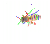
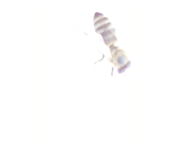
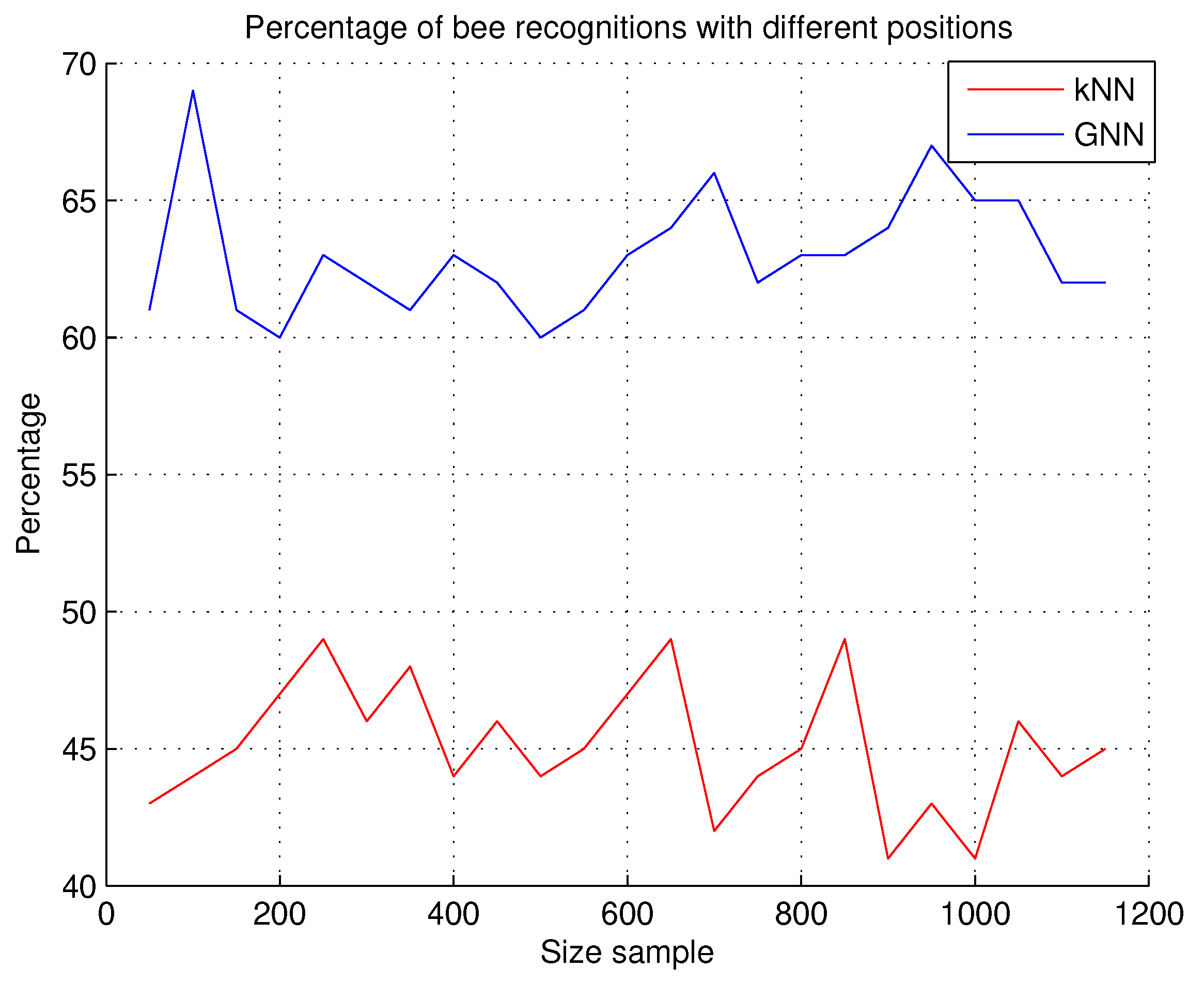
7.2.9. Recognition of Bees with Different Positions

A determining factor for the system to recognize the bee and locate the Varroa mite is the position of the bee at the hive entrance. The bee can have many different positions at the hive entrance, as shown in some examples of the dataset in Table 7; these different positions of the bee must be verified by the software system; so, in this experiment, we used the kNN and GNN techniques to evaluate the recognition percentages of bees with different positions.

Observations. The results are shown in Figure 17; the recognition accuracy that we obtained with the GNN technique is higher, as shown by the results of the graphed percentages. A lower accuracy is obtained with the kNN technique.

8. Limitations

In this section, technical and practical limitations of this research project are highlighted. Among technical limitations, three have been found, which are described below.

First, one limitation is the location of the apiaries, which for safety reasons must be located at distances greater than 800 m from the passage of humans and animals; for the development of the research, this has been considered a limitation because the system requires the installation of telecommunications devices that link the apiary with the data-processing center for its operation in real time. Second, considering the development of mobile applications with smartphones, it is possible to take advantage of the telephone network that reaches more distant places, but in our country, there are still many places without access to the telephone network. Third, there is still no portable device (device container) that contains all the devices that are installed in the hive, so the design of a portable device that can be easily transported to apiaries should be considered; the proposed portable device must be designed in such a way that it is noninvasive, in order to respect the life and work of honeybees.

The practical limitations of this project are the transportation of the devices to test apiaries and days with rainy weather. Transporting the devices to test apiaries is a strenuous activity, due to the distances that must be traveled to reach the target site. With respect to rainy days, it is not possible to carry out tests in test apiaries because the bees choose not to leave the hive, so there is no transit of bees through the entrance.

9. Conclusions

In this research, an automatic recognition system for honeybee recognition in real environments was presented, as well as a subsequent analysis of the bee’s thorax to detect ectoparasites. The proposed method uses digital image processing, a technique for generating embedding vectors, and two techniques that are used in the recognition phase: k-Nearest Neighbors (kNN), a versatile classifier, and Graph Neural Network (GNN). Results obtained show the versatility of each technique. Although kNN shows more false positives than GNN, it is a technique that we consider appropriate for real-time environments, due to the speed of response during processing; GNN is a novel recognition technique, and processing requires a longer time. kNN is a versatile and fast classifier, but with lower recognition rates, which makes it more likely to make errors. Experiments were described with the objective of carrying out the recognition of honeybees in hives and a subsequent analysis of the thorax, to detect ectoparasites in real environments. Additionally, in this work, we have addressed two problems inherent to object recognition. First, there is the problem encountered with the positions taken by bees at the entrance of the hive. Although an attempt is proposed to solve the positions in [13], there are still many challenges and it is necessary to propose other techniques that achieve recognition of images of bees in different positions and incomplete images of bees; second, there is the issue of the environments in real apiaries where the project is applied. In these environments, the lighting conditions play a predominant role in the recognition of honeybees.

10. Future Works

Once this work is finished, there are three future tasks that have been proposed to continue the research: first, to extract more examples from real apiaries with more devices, which will allow us to perform exhaustive training of the neural network to increase the percentages of recognition of honeybees with both techniques. Second, due to the limitations of the installation of telecommunications devices in the test apiaries, the use of cellular telephone technology to link the remote sites (test apiaries) with the data-processing center is proposed; the costs of using this technology are currently being considered. Finally, as shown in Table 7, the images acquired at the entrance to the beehive do not show the full body of the hive, so we are currently working on modifications to the software system for recognition in more complex conditions, with bees that are not complete in the image.

11. Discussion

In this section, discussions of the presented research project have focused on the feasibility of the project and our contributions to the state of the art of the problem of Varroa detection in honeybees, the criteria used to evaluate the proposed methodology, and what have been the practical limitations that we have had for the development of this research work applied to beekeeping.

As a discussion, the following question is proposed: How do our experimental results demonstrate the feasibility of using digital image processing for bee recognition in real apiary environments? The results obtained with the applied techniques and the method proposed in this research work demonstrate the feasibility of developing an automatic recognition system in real honeybee environments; based on the experiments proposed and discussed in this work, we consider that the results obtained with both techniques (even with percentages lower than 80%) are acceptable for real environments.

Making a comparison between the results presented in other works in the literature, the results presented and described in this work are acceptable and demonstrate the feasibility of developing the automatic recognition system and applying it in real environments; the criteria we have considered to ensure that our research is feasible are listed below.

• The development of a real-time system. We do not use any images in controlled environments, as many other works do, to offer very high recognition results; we extract the visual information from the apiary with different climatic situations, excluding only rainy days to protect our image and video capture equipment.
• We present a noninvasive system in the hive. The main focus of our system was to develop noninvasive technology in the hive, to avoid stress to the bees, and not sacrifice any insect in the colony.
• We developed an economic and fast system with efficient devices. The beekeeping community is not willing to spend large amounts of money on new technology, which led us to develop a system with low cost and accessible but fast devices.
• The software is our own creation; the software is developed with freely available technologies, such as the C language, OpenCV, which runs on free operating systems and allows the student community of the university to offer examples of the use of this software, such as Linux in its different flavors.
• The creation of four datasets that grow indefinitely as they acquire the images from the test apiaries. With these datasets, we have managed to train the proposed neural network with a large number of possible occurrences of the Varroa mite, which allows us to announce to the beekeeper community the possible cases of infection with the Varroa parasite.
• The community of beekeepers in the region where the project is being carried out has requested the demonstration of the functionality of the project due to the results that have been published in different international scientific events and journals, such as [13,34].

In previous reviews of this work, we have been asked what the contributions are to the state of the art of the problem of Varroa mite detection in honeybees; we consider that this research contributes to two areas of applied research:

(a)

The development of an automatic recognition system that includes advanced techniques of artificial intelligence and the Internet of Things, and

(b)

experiments in uncontrolled natural environments of honeybees that allow the discovery and documentation of the factors that affect image acquisition in automatic recognition.

Both areas allow us to develop technology in an area that is not documented in the literature in Mexico.

Based on the above, we consider our work to be innovative and a solution to the care and preservation of honeybees in our country. No work has been presented in this area with an innovation of this magnitude, which provides an application model, as well as an academic model for university students in our country in the areas of agricultural biotechnology and information and communications technologies.

12. Patents

This research project is in the process of obtaining a patent and it is registration.

References

1. Requier, F.; Garnery, L.; Kohl, P.L.; Njovu, H.K.; Pirk, C.W.; Crewe, R.M.; Steffan-Dewenter, I. The conservation of native honey bees is crucial. Trends Ecol. Evol. 2019, 34, 789–798. [Google Scholar] [CrossRef]
2. Zhu, Y.; Yao, J.; Wang, Y. Varroa mite and deformed wing virus infestations interactively make honey bees (Apis mellifera) more susceptible to insecticides. Environ. Pollut. 2022, 292, 118212. [Google Scholar] [CrossRef]
3. Molineri, A.I.; Pacini, A.; Giacobino, A.; Bulacio-Cagnolo, N.; Aignasse, A.; Zago, L.; Fondevila, N.; Ferrufino, C.; Merke, J.; Orellano, E.; et al. Prevalence of honey bee (Apis mellifera) viruses in temperate and subtropical regions from Argentina. Rev. Argent. Microbiol. 2017, 49, 166–173. [Google Scholar] [CrossRef]
4. Namayanja, D.; Akol, A.M.; Kugonza, D.R. Prevalence of Varroa Mite Infestations Among Honey Bee Colonies in Uganda; RUFORUM Working Document Series No. 14; Makerere University Repositor: Kampala, Uganda, 2016; pp. 459–465. ISSN 1607-9345. Available online: http://repository.ruforum.org (accessed on 26 April 2023).
5. Bava, R.; Castagna, F.; Palma, E.; Ceniti, C.; Millea, M.; Lupia, C.; Britti, D.; Musella, V. Prevalence of Varroa destructor in Honeybee (Apis mellifera) Farms and Varroosis Control Practices in Southern Italy. Microorganisms 2023, 11, 1228. [Google Scholar] [CrossRef]
6. Jack, C.J.; Ellis, J.D. Integrated Pest Management Control of Varroa destructor (Acari: Varroidae), the Most Damaging Pest of (Apis mellifera L. (Hymenoptera: Apidae)) Colonies. J. Insect Sci. 2021, 21, 6. [Google Scholar] [CrossRef] [PubMed]
7. Nekoei, S.; Rezvan, M.; Khamesipour, F.; Mayack, C.; Molento, M.B.; Revainera, P.D. A systematic review of honey bee (Apis mellifera, Linnaeus, 1758) infections and available treatment options. Vet. Med. Sci. 2023, 9, 1848–1860. [Google Scholar] [CrossRef] [PubMed] [PubMed Central]
8. Schurischuster, S.; Remeseiro, B.; Radeva, P.; Kampel, M. A Preliminary Study of Image Analysis for Parasite Detection on Honey Bees. In Image Analysis and Recognition. ICIAR 2018; Campilho, A., Karray, F., ter Haar Romeny, B., Eds.; Lecture Notes in Computer Science; Springer: Cham, Switzerland, 2018; Volume 10882. [Google Scholar] [CrossRef]
9. Voudiotis, G.; Moraiti, A.; Kontogiannis, S. Deep Learning Beehive Monitoring System for Early Detection of the Varroa Mite. Signals 2022, 3, 506–523. [Google Scholar] [CrossRef]
10. Método para Determinar Niveles de Varroa en Terreno. 2021. Available online: https://teca.apps.fao.org/teca/pt/technologies/8663 (accessed on 1 August 2023).
11. König, A. IndusBee 4.0—Integrated intelligent sensory systems for advanced bee hive instrumentation and hive keepers’ assistance systems. Sens. Transducers 2019, 237, 109–121. [Google Scholar]
12. Dietemann, V.; Nazzi, F.; Martin, S.J.; Anderson, D.L.; Locke, B.; Delaplane, K.S.; Ellis, J.D. Standard methods for varroa research. J. Apic. Res. 2013, 52, 1–54. [Google Scholar] [CrossRef]
13. Velarde Martinez, A.; Rodriguez, G.G.; Cabral, J.C.E.; Moreira, J.D.R. Varroa Mite Detection in Honey Bees with Artificial Vision. In Advances in Soft Computing. MICAI 2023; Calvo, H., Martinez-Villasenor, L., Ponce, H., Eds.; Lecture Notes in Computer Science; Springer: Cham, Switzerland, 2023; Volume 14392. [Google Scholar] [CrossRef]
14. Campbell, J.; Mummert, L.B.; Sukthankar, R. Video Monitoring of Honey Bee Colonies at the Hive Entrance. Conference Proceedings. In Proceedings of the 19th International Conference on Pattern Recognition (ICPR2008), Tampa, FL, USA, 7 December 2008; Available online: https://homepages.inf.ed.ac.uk/rbf/VAIB08PAPERS/vaib9_mummert.pdf (accessed on 1 January 2023).
15. Babic, Z.; Pilipovic, R.; Risojevic, V.; Mirjanic, G. Pollen Bearing Honey Bee Detection in Hive Entrance Video Recorded by Remote Embedded System for Pollination Monitoring. ISPRS Ann. Photogramm. Remote Sens. Spat. Inf. Sci. 2016, III7, 51–57. [Google Scholar] [CrossRef]
16. Hendrikx, P.; Chauzat, M.; Debin, M.; Neuman, P.; Fries, I.; Ritter, W.; Brown, M.; Mutinelli, F.; Conte, Y.L.; Gregorc, A. Scientific Report Submitted to EFSA Bee Mortality and Bee Surveillance in Europe. Available online: https://efsa.onlinelibrary.wiley.com/doi/pdfdirect/10.2903/sp.efsa.2009.EN-27 (accessed on 25 August 2022).
17. Lee, K.; Steinhauer, N.; Travis, D.A.; Meixner, M.D.; Deen, J.; van Engelsdorp, D. Honey bee surveillance: A tool for understanding and improving honey bee health. Curr. Opin. Insect Sci. 2015, 10, 37–44. [Google Scholar] [CrossRef]
18. König, A. First results of the BeE-nose on mid-term duration hive air monitoring for Varroa infestation level estimation. Sens. Transducers 2021, 250, 39–43. [Google Scholar]
19. Sevin, S.; Tutun, H.; Mutlu, S. Detection of Varroa mites from honey bee hives by smart technology Var-Gor: A hive monitoring and image processing device. Turk. J. Vet. Anim. Sci. 2021, 45, 487–491. [Google Scholar] [CrossRef]
20. Bilik, S.; Kratochvila, L.; Ligocki, A.; Bostik, O.; Zemcik, T.; Hybl, M.; Horak, K.; Zalud, L. Visual Diagnosis of the Varroa Destructor Parasitic Mite in Honeybees Using Object Detector Techniques. Sensors 2021, 21, 2764. [Google Scholar] [CrossRef]
21. Bjerge, K.; Frigaard, C.E.; Mikkelsen, P.H.; Nielsen, T.H.; Misbih, M.; Kryger, P. A computer vision system to monitor the infestation level of Varroa destructor in a honeybee colony. Comput. Electron. Agric. 2019, 164, 104898. [Google Scholar] [CrossRef]
22. Divasón, J.; Romero, A.; Martinez-de-Pison, F.J.; Casalongue, M.; Silvestre, M.A.; Santolaria, P.; Yániz, J.L. Analysis of Varroa Mite Colony Infestation Level Using New Open Software Based on Deep Learning Techniques. Sensors 2024, 24, 3828. [Google Scholar] [CrossRef]
23. De-Melo, A.A.M.; de Almeida-Muradian, L.B.; Sancho, M.T.; Pascual-Maté, A. Composition and properties of Apis mellifera honey: A review. J. Apic. Res. 2017, 57, 5–37. [Google Scholar] [CrossRef]
24. Wu, X.; Sahoo, D.; Hoy, S.C.H. Recent Advances in Deep Learning for Object Detection. Neurocomputing 2020, 396, 39–64. [Google Scholar] [CrossRef]
25. Yang, Z.; Li, Y.; Yang, J.; Luo, J. Action Recognition with Spatio–Temporal Visual Attention on Skeleton Image Sequences. IEEE Trans. Circuits Syst. Video Technol. 2019, 29, 2405–2415. [Google Scholar] [CrossRef]
26. Gori, M.; Monfardini, G.; Scarselli, F. A new model for learning in graph domains. In Proceedings of the 2005 IEEE International Joint Conference on Neural Networks, Montreal, QC, Canada, 31 July–4 August 2005; Volume 2, pp. 729–734. [Google Scholar] [CrossRef]
27. Scarselli, F.; Gori, M.; Tsoi, A.C.; Hagenbuchner, M.; Monfardini, G. The graph neural network model. IEEE Trans. Neural Netw. 2008, 20, 61–80. [Google Scholar] [CrossRef]
28. Vasudevan, V.; Bassenne, M.; Islam, M.T.; Xing, L. Image classification using graph neural network and multiscale wavelet superpixels. Pattern Recognit. Lett. 2023, 166, 89–96. [Google Scholar] [CrossRef]
29. Long, J.; Yan, Z.; Chen, H. A Graph Neural Network for superpixel image classification. J. Phys. Conf. Ser. 2021, 1871, 012071. [Google Scholar] [CrossRef]
30. Gong, L.; Cheng, Q. Exploiting Edge Features in Graph Neural Networks. arXiv 2019. [Google Scholar] [CrossRef]
31. Zhao, W.; Persello, C.; Stein, A. Extracting planar roof structures from very high resolution images using graph neural networks. ISPRS J. Photogramm. Remote. Sens. 2022, 187, 34–45. [Google Scholar] [CrossRef]
32. Renton, G.; Héroux, P.; Gaüzre, B.; Adam, S. Graph Neural Network for Symbol Detection on Document Images. In Proceedings of the 2019 International Conference on Document Analysis and Recognition Workshops (ICDARW), Sydney, NSW, Australia, 22–25 September 2019; pp. 62–67. [Google Scholar] [CrossRef]
33. Zhou, J.; Cui, G.; Hu, S.; Zhang, Z.; Yang, C.; Liu, Z.; Sun, M. Graph neural networks: A review of methods and applications. AI Open 2020, 1, 57–81. [Google Scholar] [CrossRef]
34. Velarde, A.; Reyes, J.; Estrada, J.; Gonzalez, G. Characterization of Honey Bee Anatomy for Recognition and Analysis Using Image Regions. Res. Comput. Sci. 2023, 152, 17–29. [Google Scholar]
35. Mourchid, Y.; El Hassouni, M.; Cherifi, H. An Image Segmentation Algorithm based on Community Detection. In Complex Networks & Their Applications V. COMPLEX NETWORKS 2016 2016; Cherifi, H., Gaito, S., Quattrociocchi, W., Sala, A., Eds.; Studies in Computational Intelligence, vol. 693; Springer: Cham, Switzerland, 2017. [Google Scholar] [CrossRef]
36. Nikolentzos, G.; Thomas, M.; Rivera, A.R.; Vazirgiannis, M. Image Classification Using Graph-Based Representations and Graph Neural Networks. Complex Networks &Their Applications IX. COMPLEX NETWORKS 2020 2020. In Studies in Computational Intelligence; Benito, R.M., Cherifi, C., Cherifi, H., Moro, E., Rocha, L.M., Sales-Pardo, M., Eds.; Springer: Cham, Switzerland, 2021; Volume 944. [Google Scholar] [CrossRef]
37. Ward, I.R.; Joyner, J.; Lickfold, C.; Guo, Y.; Bennamoun, M. A practical tutorial on graph neural networks. ACM Comput. Surv. 2022, 54, 1–35. [Google Scholar] [CrossRef]
38. Haralick, R.M. Glossary and index to remotely sensed image pattern recognition concepts. Pattern Recognit. 1973, 5, 391–403. [Google Scholar] [CrossRef]
39. Sonka, M.; Hlavac, V.; Boyle, R. Image Processing, Analysis, and Machine Vision, 4th ed.; Cengage Learning: Boston, MA, USA, 2015; ISBN -13 978-1-133-59360-7. [Google Scholar]
40. Ghaleb, O. Introduction to Maximum Matching in Graphs. Available online: http://people.scs.carleton.ca/~maheshwa/courses/5703COMP/16Fall/Matching-Report.pdf (accessed on 20 December 2022).
41. Goyal, P.; Ferrara, E. Graph embedding techniques, applications, and performance: A survey. Knowl. Based Syst. 2018, 151, 78–94. [Google Scholar] [CrossRef]
42. Singhal, P.; Verma, A. A review on graph based segmentation techniques. In Proceedings of the 10th International Conference on Intelligent Systems and Control (ISCO), Coimbatore, India, 7–8 January 2016; pp. 1–6. [Google Scholar] [CrossRef]
43. Image Processing (Imgproc Module). Available online: https://opencv.org (accessed on 20 January 2021).
44. Haralick, R.M.; Shapiro, L.G. Glossary of Computer Vision Terms. Pattern Recognit. 1991, 24, 69–93. [Google Scholar] [CrossRef]
45. Liu, Z.; Wang, H.; Zhou, T.; Shen, Z.; Kang, B.; Shelhamer, E.; Darrell, T. Exploring Simple and Transferable Recognition-Aware Image Processing. IEEE Trans. Pattern. Anal. Mach. Intell. 2022, 45, 3032–3046. [Google Scholar] [CrossRef] [PubMed]
46. Freeman, H. On the encoding of arbitrary geometric configurations. IEEE Trans. Electron. Comput. 1961, EC-10, 260–268. [Google Scholar] [CrossRef]
47. Nasien, D.; Yulianti, D.; Omar, F.S.; Adiya, M.H.; Desnelita, Y.; Chandra, T. New feature vector from freeman chain code for handwritten roman character recognition. In Proceedings of the 2nd International Conference on Electrical Engineering and Informatics (ICon EEI), Batam, Indonesia, 16–17 October 2018; pp. 67–71. [Google Scholar] [CrossRef]
Figure 1. General scheme of the beehive of Apis mellifera bees.
Applsci 15 07969 g001
Figure 2. Real suitable beehive in operation inside the apiary.
Applsci 15 07969 g002
Figure 3. The power solar system operating in real time in the beehive.
Applsci 15 07969 g003
Figure 4. The communication system between the CPD and apiary.
Applsci 15 07969 g004
Figure 5. Phases of the method that constitute the algorithm for the recognition and analysis of Apis mellifera bees.
Applsci 15 07969 g005
Figure 6. Transversal procedure in the matrix to obtain pixels with value equal 1.
Applsci 15 07969 g006
Figure 7. Process to convert the image to graph, and recognition by GNN.
Applsci 15 07969 g007
Figure 8. Complete process to neural-network training.
Applsci 15 07969 g008
Figure 9. Results of bee recognitions at the beehive entrance.
Applsci 15 07969 g009
Figure 10. Results of false positives at the beehive entrance.
Applsci 15 07969 g010
Figure 11. Results of false negatives at the beehive entrance.
Applsci 15 07969 g011
Figure 12. Results of recognition of bees with the ectoparasite Varroa.
Applsci 15 07969 g012
Figure 13. Results of false positives in bees infected with the Varroa ectoparasite.
Applsci 15 07969 g013
Figure 14. Percentages of false negatives in bees infected with the Varroa ectoparasite.
Applsci 15 07969 g014
Figure 15. Recognition time of the bee at the beehive entrance and detection of the Varroa mite.
Applsci 15 07969 g015
Figure 16. System times to recognize bees in the beehive entrance.
Applsci 15 07969 g016
Figure 17. Recognition of bees with different positions.
Applsci 15 07969 g017