
Design and Performance of a Large-Diameter Earth–Air Heat Exchanger Used for Standalone Office-Room Cooling


Abstract
1. Introduction
2. Methods
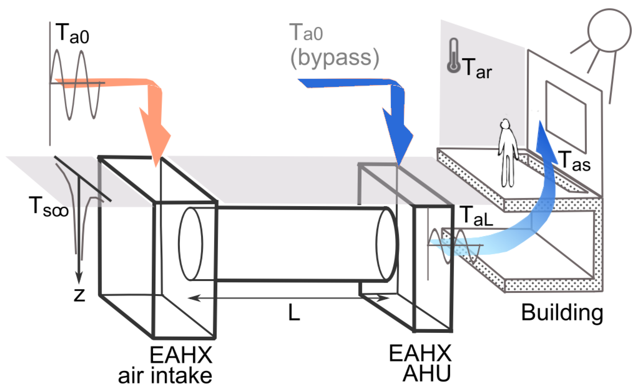
2.1. Characterization of an EAHX for Standalone Room Cooling
2.2. Constraints on the Design of Large-Diameter EAHXs for Room Load Removal
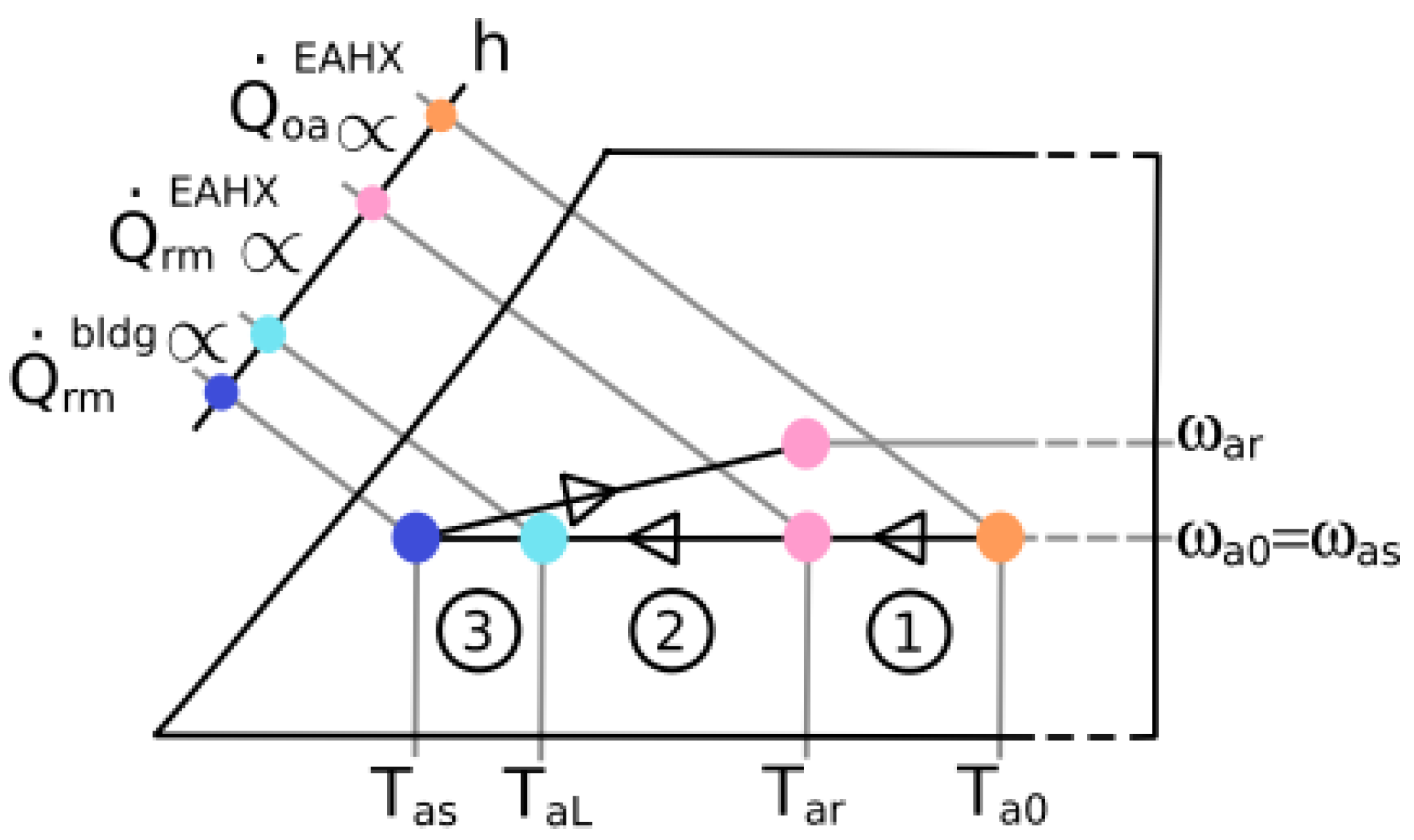
2.3. Simplified Expressions for Large-Diameter EAHX Thermal Design
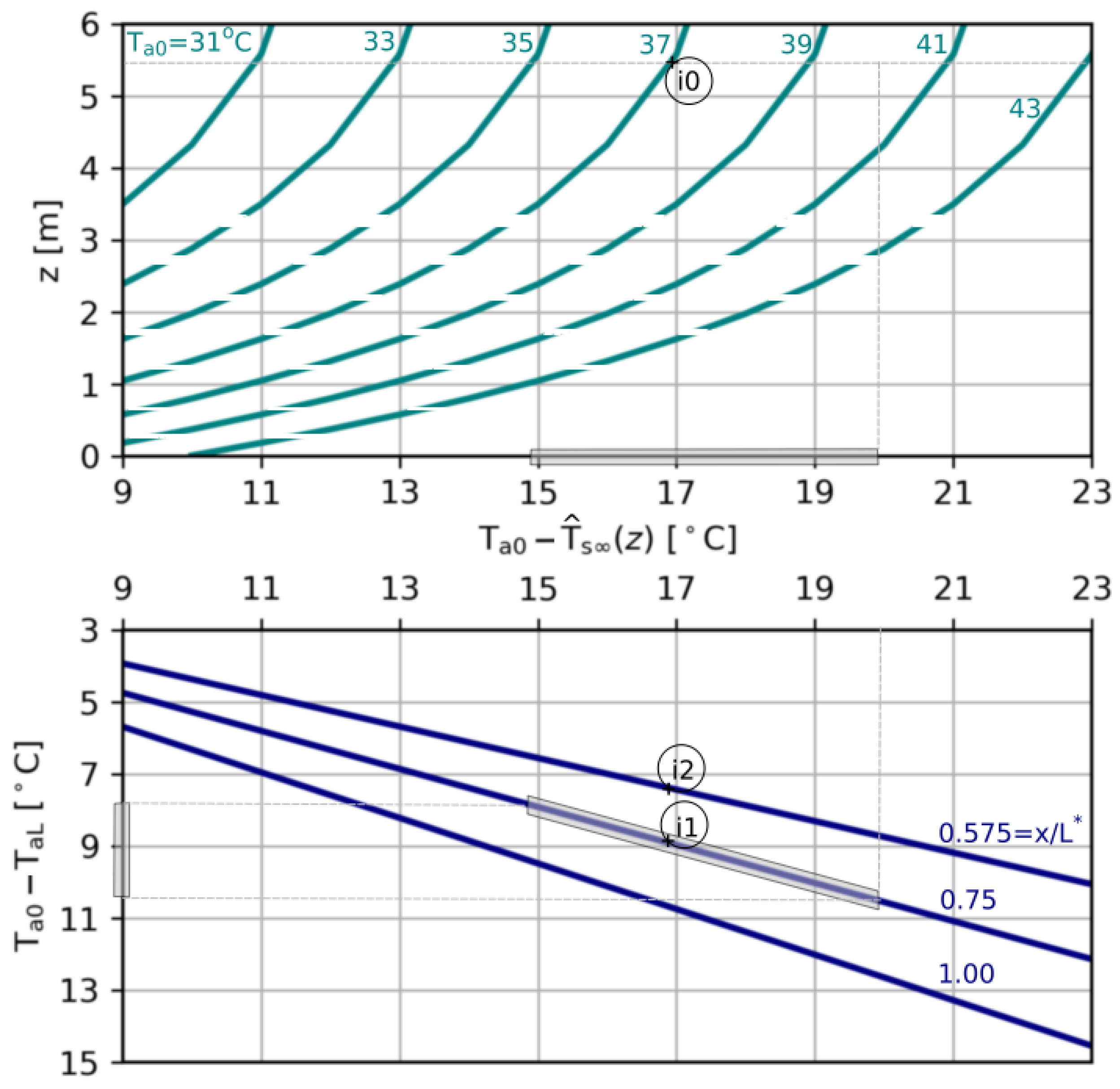
2.4. Graph-Based Design Method
- Pipe burial depth m;
- EAHX inlet air temperature: °C;
- EAHX airflow rate: .
- Pipe burial depth m;
- EAHX inlet air temperature: C;
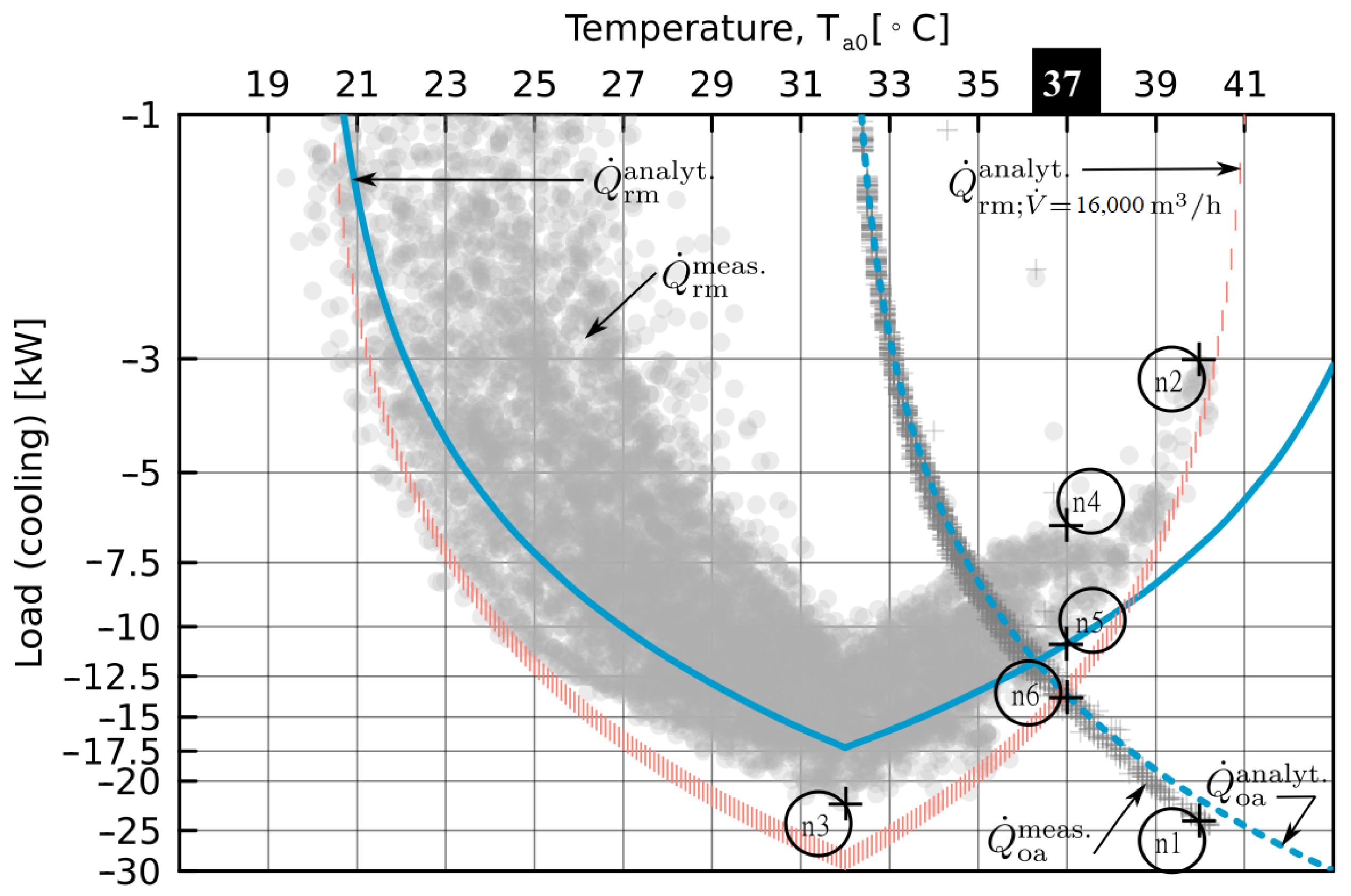
- EAHX airflow rate: = 16,000 .
3. Case Study
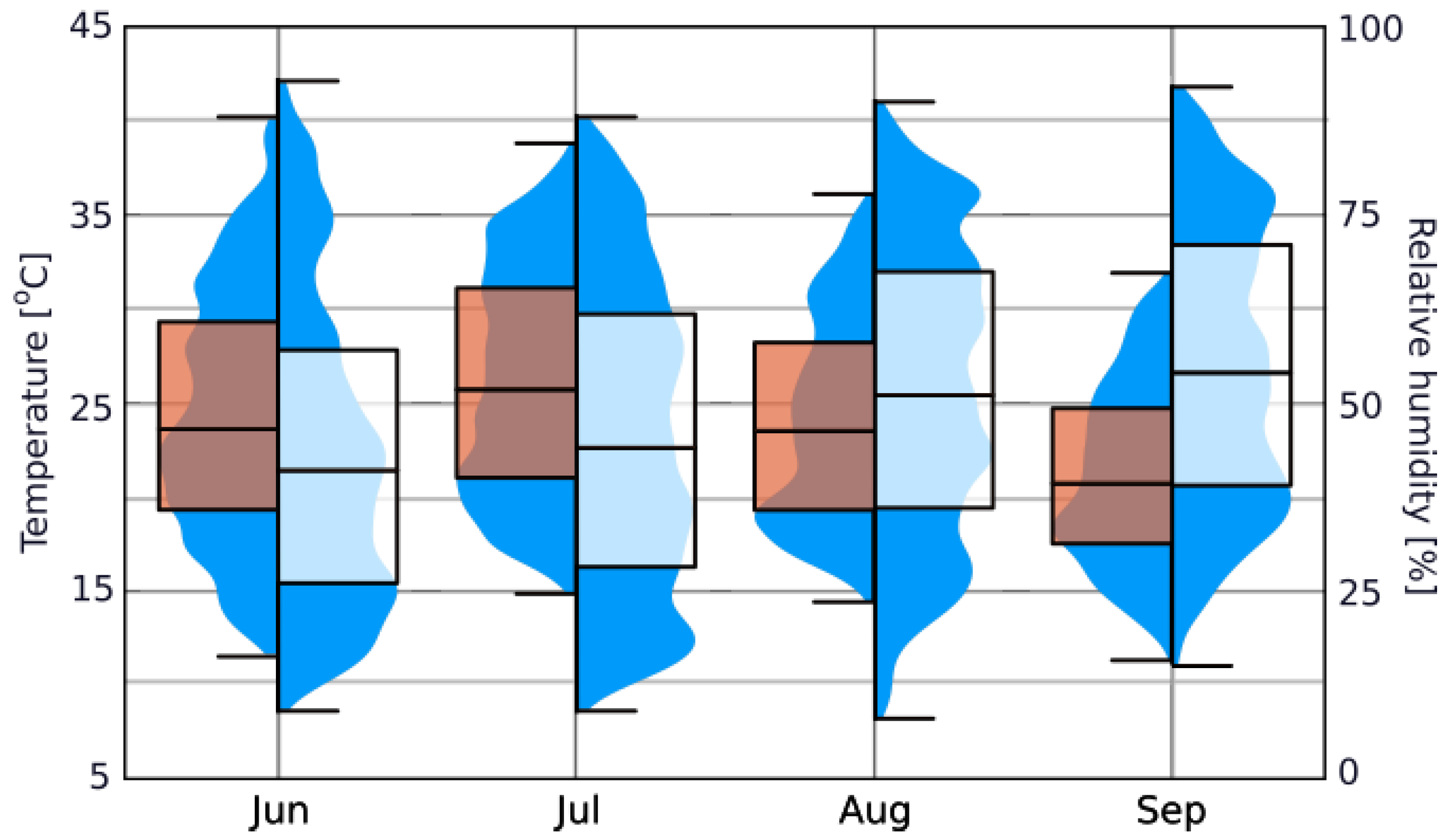
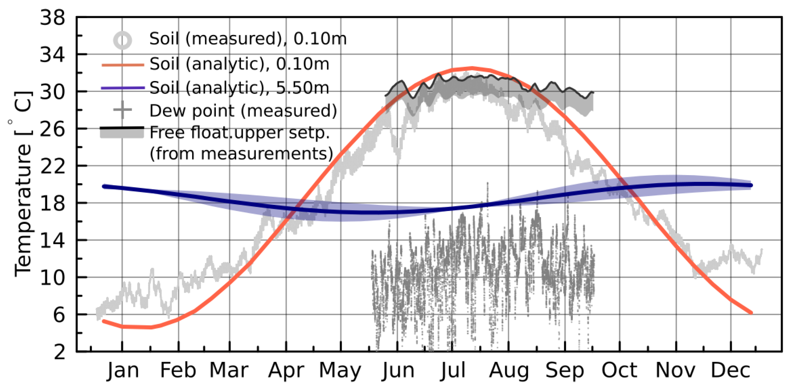
3.1. EAHX Location, Climate and Soil Temperature
3.2. The Building (Being Cooled by the EAHX)

| Bldg Parameter | Design Value | Comment |
|---|---|---|
| 1. Floor area †, | 450 m2 (EAHX cooled) | 1a. Total floor area 750 m2. |
| 2. Room height, | 3 m | 2a. Average value. |
| 3. Outdoor air temperature | 37 °C (equal to EAHX inlet temperature, ) | 3a. ASHRAE’s 0.4% annual dry bulb design value for Beja, Portugal [40]. |
| 4. Room setpoint temperature †, | 32 °C (upper limit according to data in Figure 7) | 4a. Ventilation and cooling with EAHX is handled as equivalent to natural ventilation, allowing free-floating indoor air temperatures. 4b. An adaptive comfort model is used with office room upper setpoint temperature defined from outdoor running mean temperature [28]. |
| 5. Room (air) cooling load demand †, | ∼50 W/m2 (sensible heat; considering the simultaneous sum of internal gains and gains through the building envelope) | 5a. Rooms are used for light office work; have low occupancy density; design makes use of structural elements’ thermal mass; an airtight, well-insulated envelope and glazings with appropriate solar control reduce room cooling demand. |
| 6. Room ach †, | ∼11 (100% fresh air system as in “Case 2”); 16,000 ≈ | 6a. Local draught discomfort is prevented with careful selection and placement of air supply diffusers and air extractor grilles; 6b. During summer, larger (controlled) airflow velocities in the room working area offset larger air temperatures [28]. |
| 7. Supply air temperature †, Tas | ∼4 K below the design upper free-floating setpoint temperature (C when C) | 7a. Use of building’ structural elements (foundations) thermal mass in combination with forced nighttime ventilation allows a design temperature gradient between the air supplied to the room and the air as it exits the EAHX between and K. |
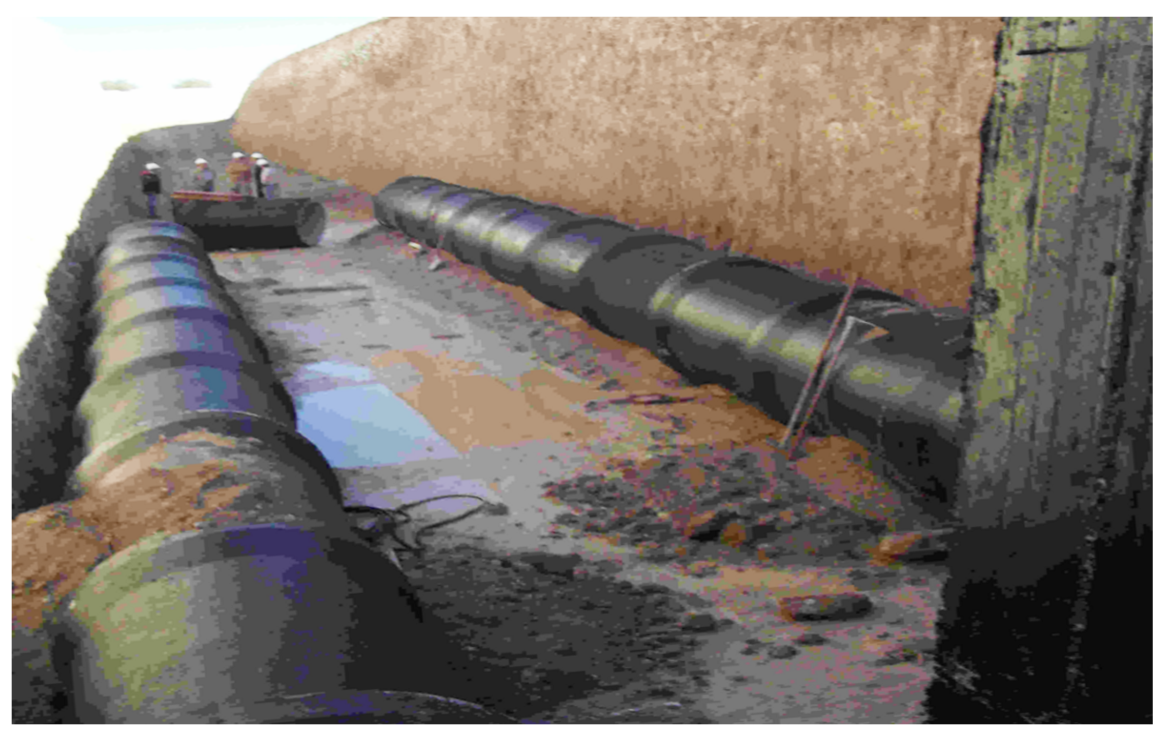
3.3. The Built EAHX and Monitoring Equipment Used
4. Results and Discussion
4.1. Monitoring Data
4.2. Evaluation of the Graph-Based Method
4.3. EAHX’s Capacity to Meet the Room Design Cooling Load Demand
5. Conclusions
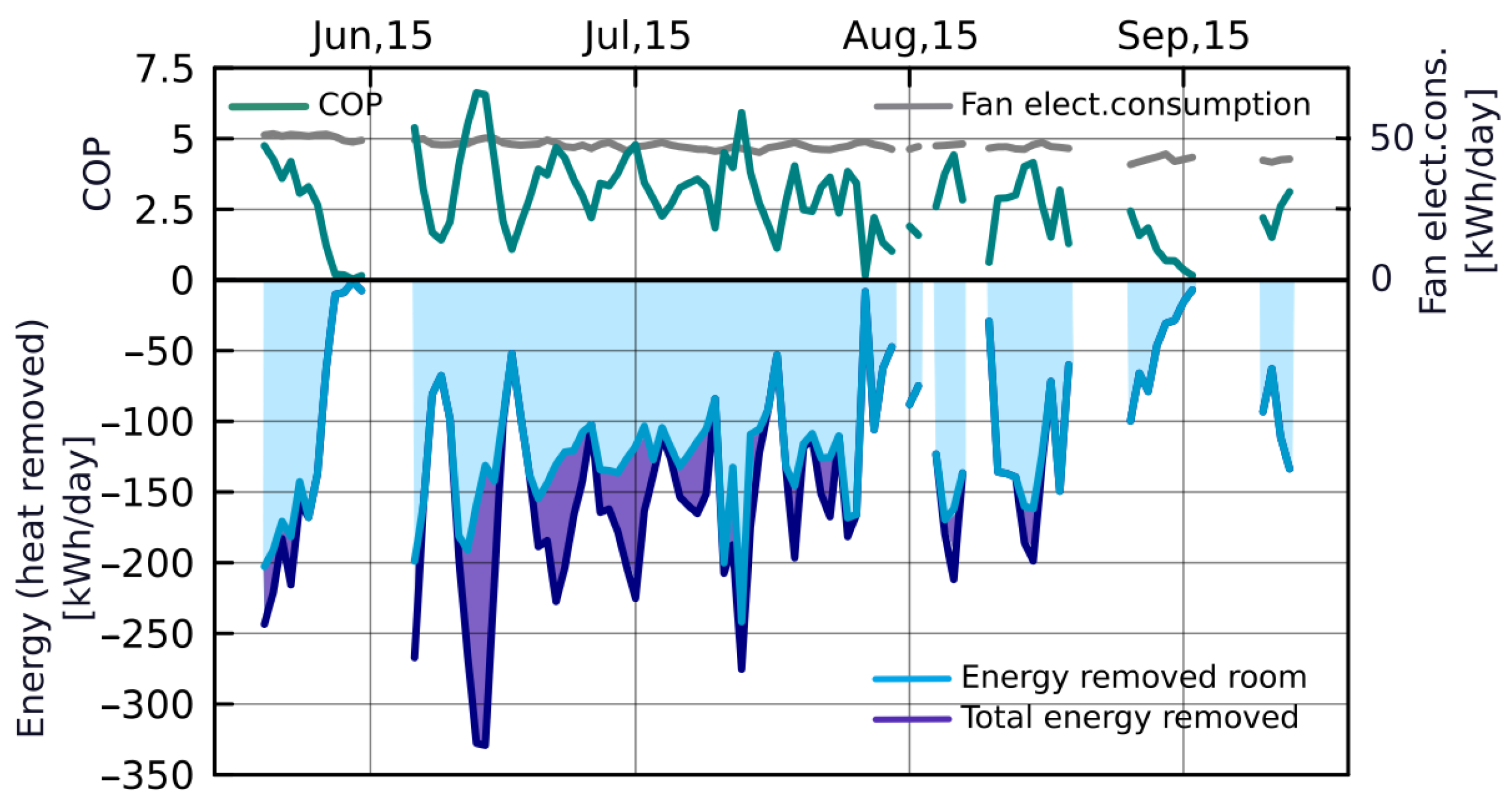
- With adequate sizing, large-diameter EAHX can remove significant room loads without the need for refrigeration machines and with little electrical energy consumption. For the monitored EAHX, a total peak cooling capacity of 28 kW and a total of 330 kWh removed in a day were achieved with just 50 kWh/day of fan electricity consumption. As regards specifically the EAHX’s ability to remove room loads—essential to assess the standalone cooling capability, a maximum value of 22 kW was monitored, i.e., the EAHX is capable of offsetting 49 W/m2 of the room cooling demand.
- Still, these results are only possible when an adaptive standard for thermal comfort is considered. Indeed, regarding the choice of the design room setpoint temperature, use of adaptive comfort models allowing setpoints higher than those for conventional HVAC systems is, most likely, mandatory when designing an EAHX for standalone use.
- Moreover, for the hottest summer days, the monitoring data showed that for hours with outdoor temperature equal to C (meeting the design condition criteria), room load removal in the EAHX reached, at best, 60% of the design cooling demand. As it happens in the design of naturally ventilated office buildings for hot and dry climates, the adoption of (building-related) passive cooling techniques, such as combining the use of building thermal mass with forced nighttime ventilation, is, most likely, also mandatory when designing an EAHX for standalone room cooling.
- Concerning the graph-based design method, the monitoring results obtained considering the design conditions were fairly matched by those determined from the graphs and from the analytical expressions supporting the graphs. This confirms that simplified analytical expressions and graphical methods can assist designers seeking an EAHE alternative to conventional HVAC solutions based on refrigeration machines.
Author Contributions
Funding
Institutional Review Board Statement
Informed Consent Statement
Data Availability Statement
Acknowledgments
Conflicts of Interest
Nomenclature
| A | area, m2 |
| c | specific heat, J/(kg K); in this paper J/(kg K) |
| D | diameter (EAHX pipe), m |
| h | height (room), m; heat transfer (convective/conduction) coefficient, W/(m2 K); |
| specific enthalpy, J/kg | |
| K | inverse of soil thermal wave relaxation distance [30], m |
| L | EAHX pipe length, m |
| mass flow rate, kg/s | |
| n | air change rate (room), s |
| heat transfer rate (cooling load), W | |
| Q | heat, kWh |
| r | radial position, m |
| R | soil radius thermally disturbed by the presence of the EAHX pipe, m |
| EAHX pipe inner radius, m | |
| t | time, s |
| T | temperature, °C (or K for temperature gradient) |
| U | convection–conduction coefficient, W/(m2 K) |
| v | velocity, m/s |
| EAHX airflow rate, m3/s | |
| W | electric energy (fan), kWh |
| x | position (along the EAHX pipe), m |
| z | depth (soil), m |
| thermal diffusivity, m2/s; in this paper m2/s | |
| efficiency (EAHX), none | |
| thermal conductivity, W/(m K); in this paper W/(m K) | |
| density, m/s; in this paper kg/m3 | |
| specific humidity, kg/kg | |
| ∝ | proportional to, none |
| Subscripts | |
| 0 | denotes initial or reference value |
| a | denotes air |
| a0 | denotes air entering the EAHX |
| aL | denotes air leaving the EAHX |
| as | denotes air supplied to a room |
| ar | denotes air in the room |
| oa | denotes outdoor air |
| rm | denotes room |
| s | denotes soil |
| s0 | denotes soil at a reference depth |
| s∞ | denotes undisturbed soil |
| t | denotes total |
| Superscripts and Abbreviations | |
| denotes nondimensional or average value | |
| denotes maximum value | |
| denotes a characteristic value | |
| denotes specific value—per unit surface | |
| ach | air change rate |
| AHU | air handling unit |
| bldg | building |
| COP | coefficient of performance |
| EAHX | earth–air heat exchanger |
| HVAC | heating, ventilation and air-conditioning |
| STP | standard temperature and pressure (273.15 K; 1.013 × Pa) |
| TM | thermal mass |
References
- Asimakopoulos, D. Passive Cooling of Buildings; James & James: London, UK, 1996. [Google Scholar] [CrossRef]
- Ferrucci, M.; Peron, F. Ancient Use of Natural Geothermal Resources: Analysis of Natural Cooling of 16th Century Villas in Costozza (Italy) as a Reference for Modern Buildings. Sustainability 2018, 10, 4340. [Google Scholar] [CrossRef]
- Mihalakakou, G.; Souliotis, M.; Papadaki, M.; Halkos, G.; Paravantis, J.; Makridis, S.; Papaefthimiou, S. Applications of earth-to-air heat exchangers: A holistic review. Renew. Sustain. Energy Rev. 2022, 155, 111921. [Google Scholar] [CrossRef]
- Soares, N.; Rosa, N.; Monteiro, H.; Costa, J. Advances in standalone and hybrid earth-air heat exchanger (EAHX) systems for buildings: A review. Energy Build. 2021, 253, 111532. [Google Scholar] [CrossRef]
- Koshlak, H. A review of earth-air heat exchangers: From fundamental principles to hybrid systems with renewable energy integration. Energies 2025, 18, 1017. [Google Scholar] [CrossRef]
- IEA. Buildings, IEA, Paris. 2022. Available online: https://www.iea.org/reports/buildings (accessed on 25 February 2025).
- Lee, K.; Strand, R. The cooling and heating potential of an earth tube system in buildings. Energy Build. 2008, 40, 486–494. [Google Scholar] [CrossRef]
- Al-Ajmi, F.; Loveday, D.; Hanby, V. The cooling potential of earth-air heat exchangers for domestic buildings in a desert climate. Build. Environ. 2006, 41, 235–244. [Google Scholar] [CrossRef]
- Michalak, P. Hourly Simulation of an Earth-to-Air Heat Exchanger in a Low-Energy Residential Building. Energies 2022, 15, 1898. [Google Scholar] [CrossRef]
- Pfafferott, J. Evaluation of earth-to-air heat exchangers with a standardised method to calculate energy efficiency. Energy Build. 2003, 35, 971–983. [Google Scholar] [CrossRef]
- D’Agostino, D.; Esposito, F.; Greco, A.; Masselli, C.; Minichiello, F. Parametric Analysis on an Earth-to-Air Heat Exchanger Employed in an Air Conditioning System. Energies 2020, 13, 2925. [Google Scholar] [CrossRef]
- Ascione, F.; Bellia, L.; Minichiello, F. Earth-to-air exchanger for Italian climates. Renew. Energy 2011, 36, 2177–2188. [Google Scholar] [CrossRef]
- Barnard, N.; Jauzens, D.E. IEA Annex 28 Subtask 2: Design Tools for Low Energy Cooling: Technology Selection and Early Design Guidance; Technical Report; Building Research Establishment: Garston, UK, 2001; Available online: http://www.ecbcs.org/Data/publications/EBC_Annex_28_technology_selection.pdf (accessed on 25 February 2025).
- Duarte, R.; Glória Gomes, M.; Moret Rodrigues, A.; Pimentel, F. A large-diameter earth-air heat exchanger (EAHX) built for standalone office room cooling: Monitoring results for hot and dry summer conditions. Appl. Sci. 2023, 13, 12134. [Google Scholar] [CrossRef]
- Amanowicz, Ł.; Wojtkowiak, J. Comparison of Single- and Multipipe Earth-to-Air Heat Exchangers in Terms of Energy Gains and Electricity Consumption: A Case Study for the Temperate Climate of Central Europe. Energies 2021, 14, 8217. [Google Scholar] [CrossRef]
- Mihalakakou, G.; Santamouris, M.; Lewis, J.; Asimakopoulos, D. On the application of the energy balance equation to predict ground temperature profiles. Sol. Energy 1997, 60, 181–190. [Google Scholar] [CrossRef]
- Bouhess, H.; Hamdi, H.; Benhamou, B.; Bennouma, A.; Hollmuller, P.; Limam, K. Dynamic simulation of an earth-to-air heat exchanger connected to a villa type house in Marrakech. In Proceedings of the 13th Conference of International Building Performance Simulation Association, Chambéry, France, 26–28 August 2013; pp. 1063–1070. [Google Scholar] [CrossRef]
- Vaz, J.; Sattler, M.; Santos, E.; Isoldi, L. Experimental and numerical analysis of an earth-air heat exchanger. Energy Build. 2011, 43, 2476–2482. [Google Scholar] [CrossRef]
- Taşdelen, F.; İhsan Dağtekin. A numerical study on cooling performance of different type earth-air heat exchangers. Renew. Energy 2025, 241, 122325. [Google Scholar] [CrossRef]
- Bansal, V.; Misra, R.; Agrawal, G.D.; Mathur, J. Performance analysis of earth-pipe-air heat exchanger for winter heating. Energy Build. 2009, 41, 1151–1154. [Google Scholar] [CrossRef]
- Tzaferis, A.; Liparakis, D. Analysis of the accuracy and sensitivity of eight models to predict the performance of earth-to-air heat exchangers. Energy Build. 1992, 18, 35–43. [Google Scholar] [CrossRef]
- EN 15241:2007; Ventilation for Buildings—Calculation Methods for Energy Losses Due to Ventilation and Infiltration in Buildings. European Committee for Standardization: Brussels, Belgium, 2007.
- Zimmermann, M. Handbuch der Passiven Külung; Technical Report; im Auftrag des Bundesamtes für Energie (Bern), EMPA: Dübendorf, Switzerland, 1999. [Google Scholar]
- AG Solar. Luft-Erdwärmetauscher L-EWT: Teil 1 Systeme für Wohngebäude; AG Solar: Nordrhein-Westfalen, Germany, 2025. [Google Scholar]
- Huber, A. Benutzerhandbuch zum Programm WKM (Version 3.9): Auslegung von Luft-Erdregister; Huber Energietechnik AG Ingenieurund Planungsbüro: Zürich, Switzerland, 2021. [Google Scholar]
- CanmetENERGY. Earth to Air Thermal Exchnager (EATEX): Design Principles and Concept Design Tool; Buildings and Renewables Group: Ottawa, ON, Canada, 2025. [Google Scholar]
- Peretti, C.; Zarrella, A.; De Carli, M.; Zecchin, R. The design and environmental evaluation of earth-to-air heat exchangers (EAHE). A literature review. Renew. Sustain. Energy Rev. 2013, 28, 107–116. [Google Scholar] [CrossRef]
- EN 15251:2007; Indoor Environmental Input Parameters for Design and Assessment of Energy Performance of Buildings Addressing Indoor Air Quality, Thermal Environment, Lighting and Acoustics. European Committee for Standardization: Brussels, Belgium, 2007; Currently EN 16798-1:2019.
- Maerefat, M.; Haghighi, A. Passive cooling of buildings by using integrated earth to air heat exchanger and solar chimney. Renew. Energy 2010, 35, 2316–2324. [Google Scholar] [CrossRef]
- Givoni, B.; Katz, L. Earth temperatures and underground buildings. Energy Build. 1985, 8, 15–25. [Google Scholar] [CrossRef]
- Sodha, M.; Sharma, A.; Singh, S.; Bansal, N.; Kumar, A. Evaluation of an earth-air tunnel system for cooling/heating of a hospital complex. Build. Environ. 1985, 20, 115–122. [Google Scholar] [CrossRef]
- Do, S.L.; Baltazar, J.C.; Haberl, J. Potential cooling savings from a ground-coupled return-air duct system for residential buildings in hot and humid climates. Energy Build. 2015, 103, 206–215. [Google Scholar] [CrossRef]
- Recknagel, H.; Sprenger, E.; Schramek, E. Taschenbuch für Heizung und Klimatechnik; Oldenbourg Industrieverlag: München, Germany, 2009. [Google Scholar]
- Hollmuller, P. Analytical characterisation of amplitude-dampening and phase-shifting in air/soil heat-exchangers. Int. J. Heat Mass Transf. 2003, 46, 4303–4317. [Google Scholar] [CrossRef]
- De Paepe, M.; Janssens, A. Thermo-hydraulic design of earth-air heat exchangers. Energy Build. 2003, 35, 389–397. [Google Scholar] [CrossRef]
- Duarte, R.; Moret Rodrigues, A.; Pimentel, F.; Glória Gomes, M. Supplementary Material for the Paper “Design and Performance of a Large-Diameter Earth-Air Heat Exchanger Used for Standalone Office-Room Cooling”. 2025. Available online: https://zenodo.org/records/15763007 (accessed on 28 June 2025).
- IPMA. Climate Normals—Köppen Climatic Classification. Available online: https://www.ipma.pt/en/oclima/normais.clima (accessed on 1 January 2023).
- ESDAC. EU Soil Observatory. 2025. Available online: https://esdac.jrc.ec.europa.eu/ (accessed on 12 March 2025).
- Hollmuller, P.; Lachal, B. Air-soil heat exchangers for heating and cooling of buildings: Design guidelines, potentials and constraints, system integration and global energy balance. Appl. Energy 2014, 119, 476–487. [Google Scholar] [CrossRef]
- ASHRAE. ASHRAE Handbook, Fundamentals. 2021. Available online: https://www.ashrae.org/technical-resources/ashraehandbook/ashrae-handbook-online (accessed on 25 February 2025).
- Vaisala. Vaisala Weather Transmitter WXT520—User’s Guide; Vaisala Oyj: Vantaa, Finland, 2012; Available online: https://www.vaisala.com/sites/default/files/documents/M210906EN-C.pdf (accessed on 1 January 2023).
- Onset. HOBO 4-Channel Analog Data Logger (UX120-006M) Manual. Available online: https://www.onsetcomp.com/resources/documentation/17384-c-ux120-006m-manual (accessed on 1 January 2023).
- Onset. HOBO Energy Logger: Data Logger and Modules User’s Guide. Available online: https://www.onsetcomp.com/resources/documentation/9857-man-h22-web (accessed on 1 January 2023).
- Vegetronix. THERM200 Soil Temperature Probe. Available online: https://www.vegetronix.com/Products/THERM200/ (accessed on 1 January 2023).


| Measured | Analytical (Case 1) 8000 m3/h; | Analytical (Case 2) 16,000 m3/h; | ||
|---|---|---|---|---|
| Point(s) in Figure 11 [kW] [W/m2] | ∼ 7∼11 15.5∼24.4 | 11 24.4 | 13.75 30.5 | |
| Point(s) in Figure 11 [kW] [W/m2] | 13.75 30.5 | 13.75 30.5 | — |
Disclaimer/Publisher’s Note: The statements, opinions and data contained in all publications are solely those of the individual author(s) and contributor(s) and not of MDPI and/or the editor(s). MDPI and/or the editor(s) disclaim responsibility for any injury to people or property resulting from any ideas, methods, instructions or products referred to in the content. |
© 2025 by the authors. Licensee MDPI, Basel, Switzerland. This article is an open access article distributed under the terms and conditions of the Creative Commons Attribution (CC BY) license (https://creativecommons.org/licenses/by/4.0/).
Share and Cite
Duarte, R.; Moret Rodrigues, A.; Pimentel, F.; Gomes, M.d.G. Design and Performance of a Large-Diameter Earth–Air Heat Exchanger Used for Standalone Office-Room Cooling. Appl. Sci. 2025, 15, 7938. https://doi.org/10.3390/app15147938
Duarte R, Moret Rodrigues A, Pimentel F, Gomes MdG. Design and Performance of a Large-Diameter Earth–Air Heat Exchanger Used for Standalone Office-Room Cooling. Applied Sciences. 2025; 15(14):7938. https://doi.org/10.3390/app15147938
Chicago/Turabian StyleDuarte, Rogério, António Moret Rodrigues, Fernando Pimentel, and Maria da Glória Gomes. 2025. "Design and Performance of a Large-Diameter Earth–Air Heat Exchanger Used for Standalone Office-Room Cooling" Applied Sciences 15, no. 14: 7938. https://doi.org/10.3390/app15147938
APA StyleDuarte, R., Moret Rodrigues, A., Pimentel, F., & Gomes, M. d. G. (2025). Design and Performance of a Large-Diameter Earth–Air Heat Exchanger Used for Standalone Office-Room Cooling. Applied Sciences, 15(14), 7938. https://doi.org/10.3390/app15147938