
Explainable Machine Learning for Mapping Rainfall-Induced Landslide Thresholds in Italy

 , , , ,
Abstract
1. Introduction
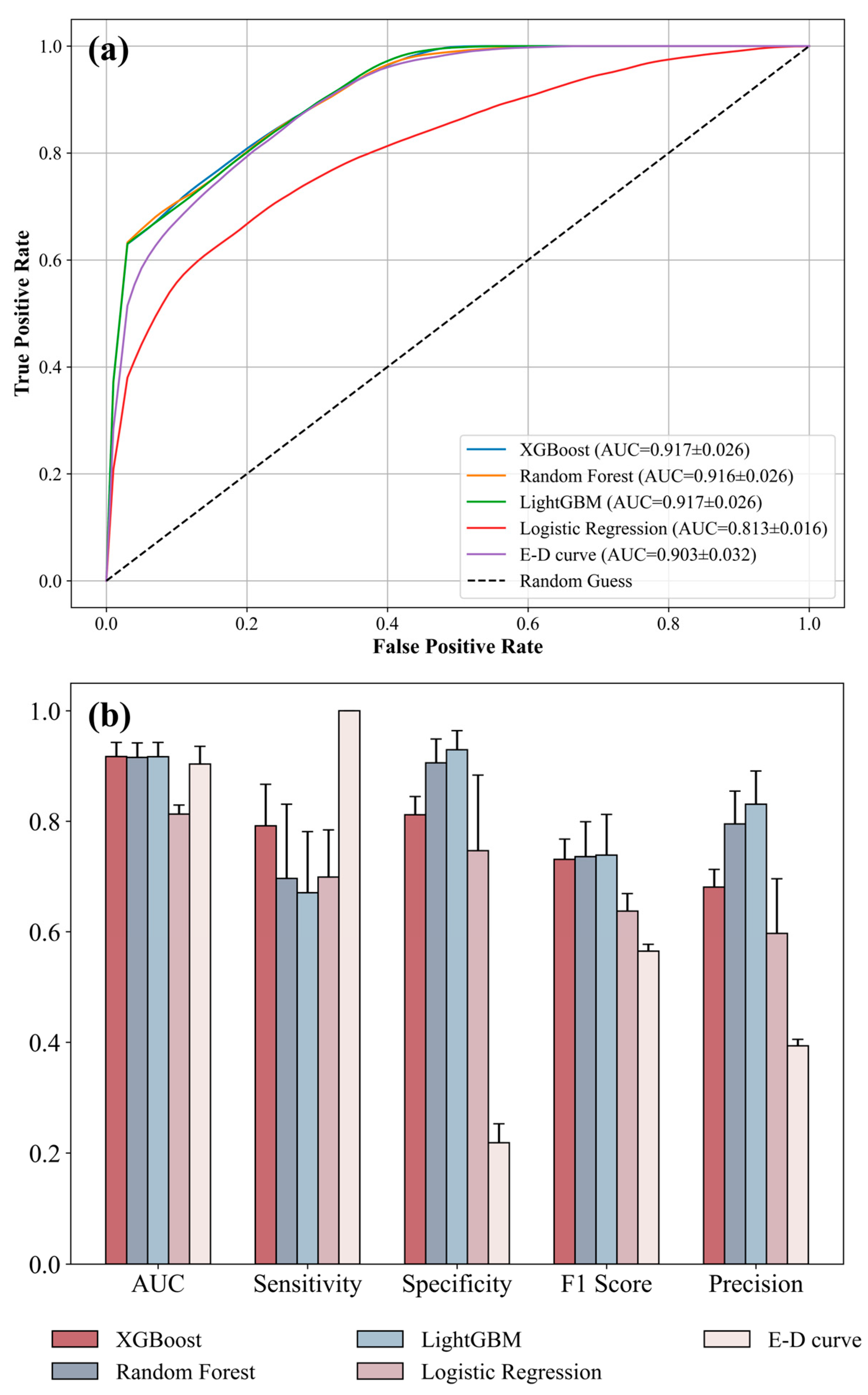
- We compared the predictive performance of empirical threshold models with four machine learning models on imbalanced datasets. The XGBoost model achieved optimal overall predictive performance and effectively balanced sensitivity and specificity;
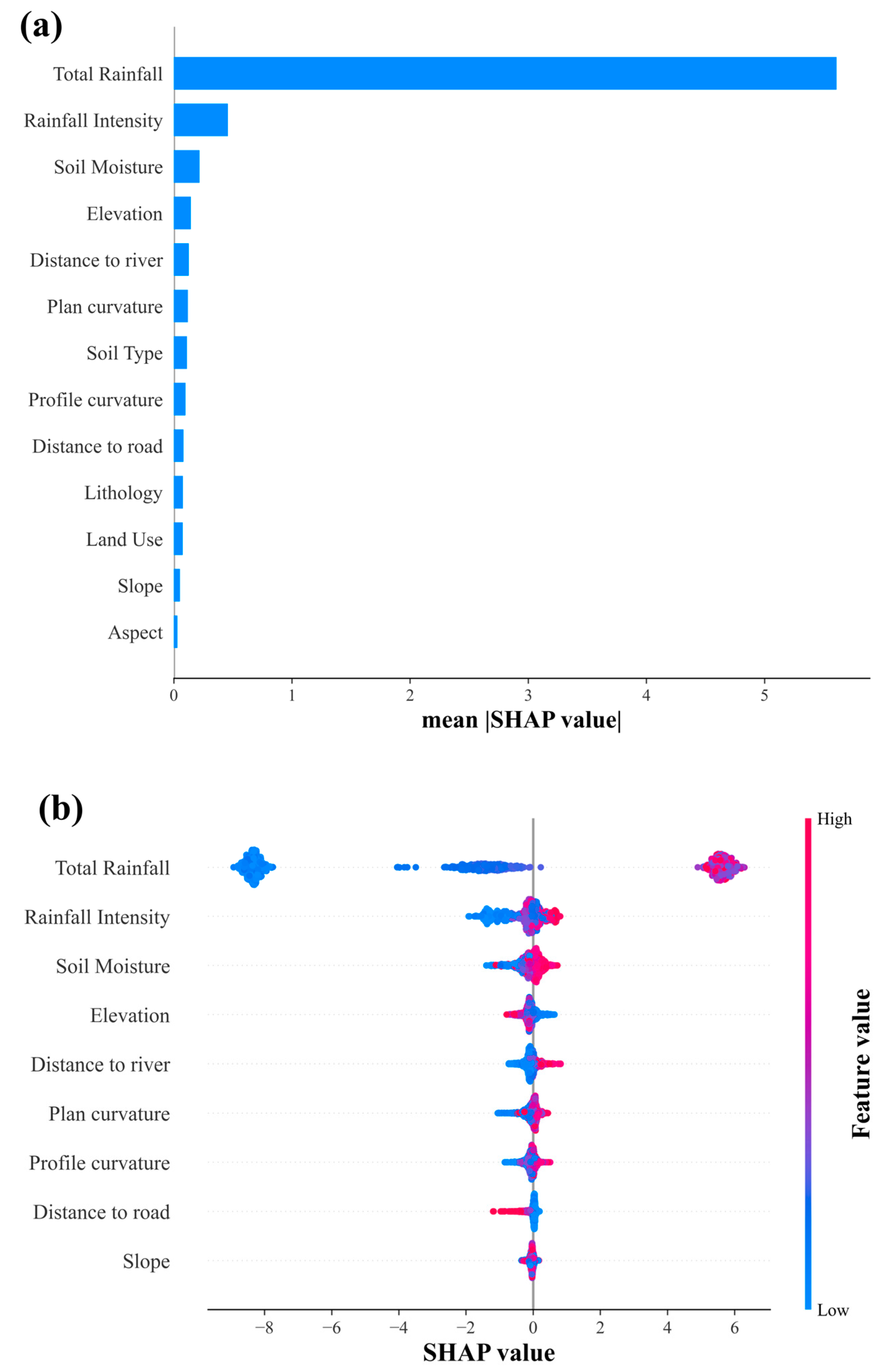
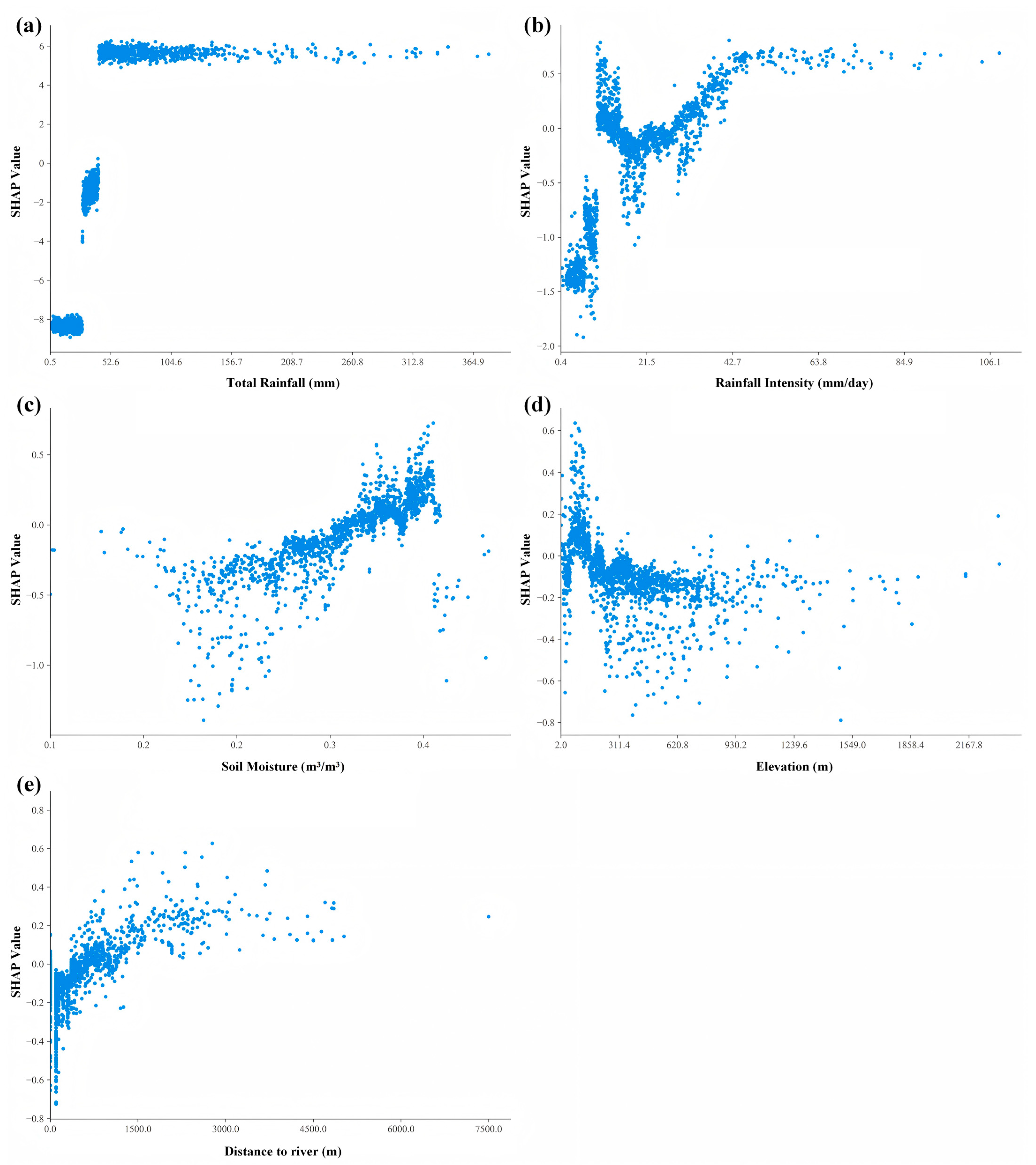
- The SHAP methodology was employed to enhance the interpretability of the machine learning model, which helped clarify the model’s decision-making process. The results indicate that hydrological factors, particularly total rainfall, play a central role in the modeling process.
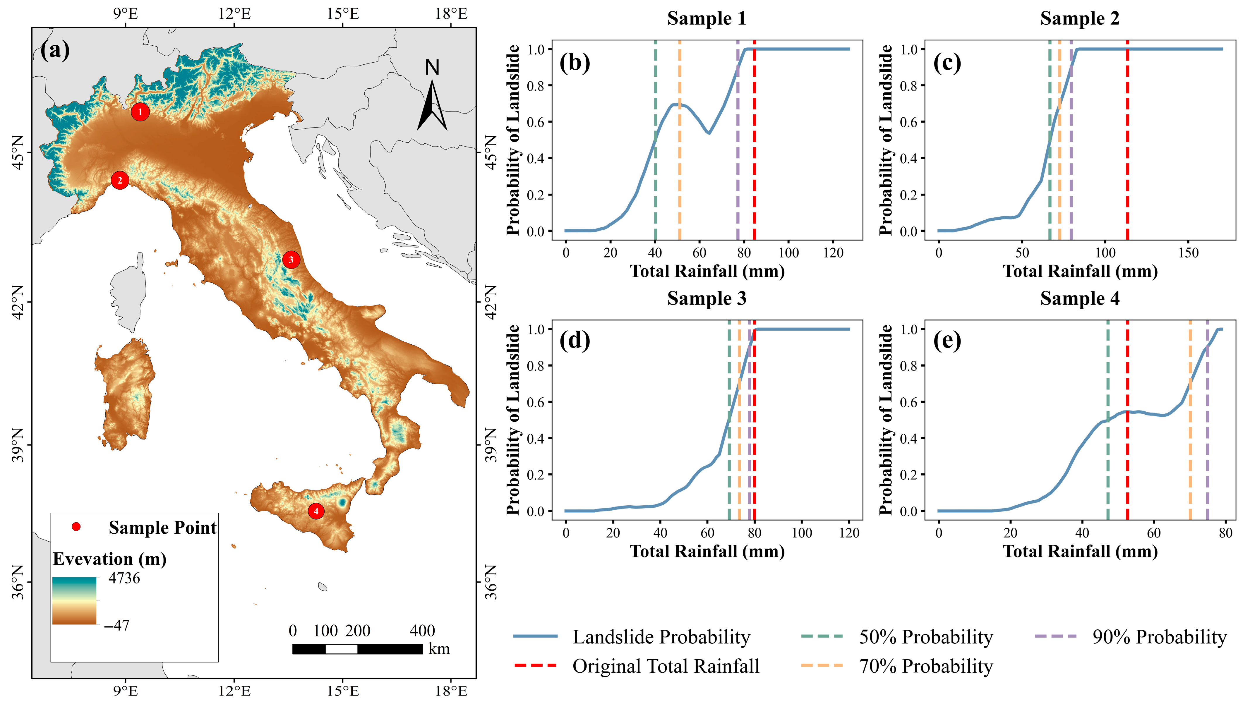
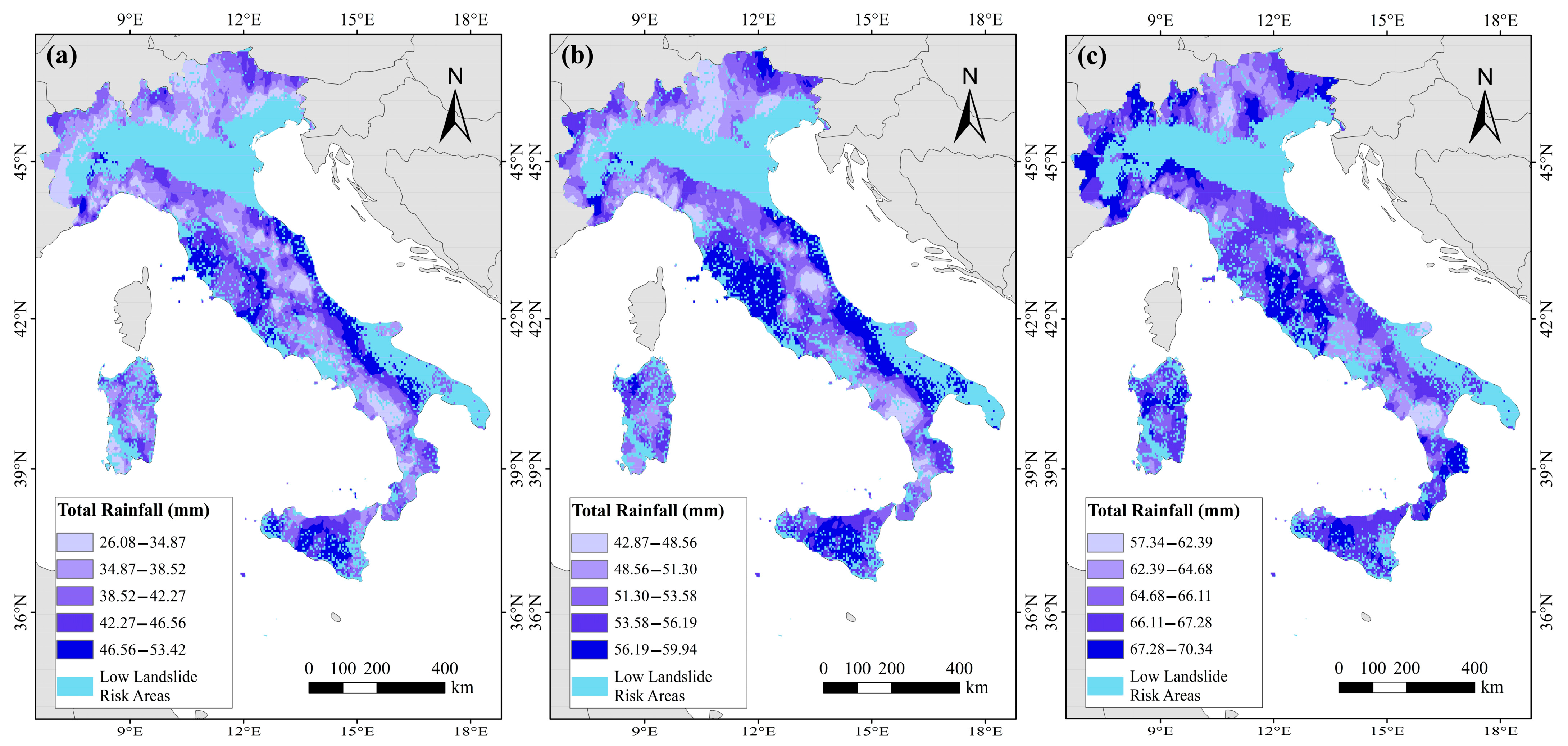
- Using the trained XGBoost model, we generated rainfall threshold maps for the Italian region under three different probability scenarios.
- This study established an intuitive and practical modeling framework for regional rainfall threshold development, offering reference for subsequent studies.
2. Study Area, Data, and Methodology
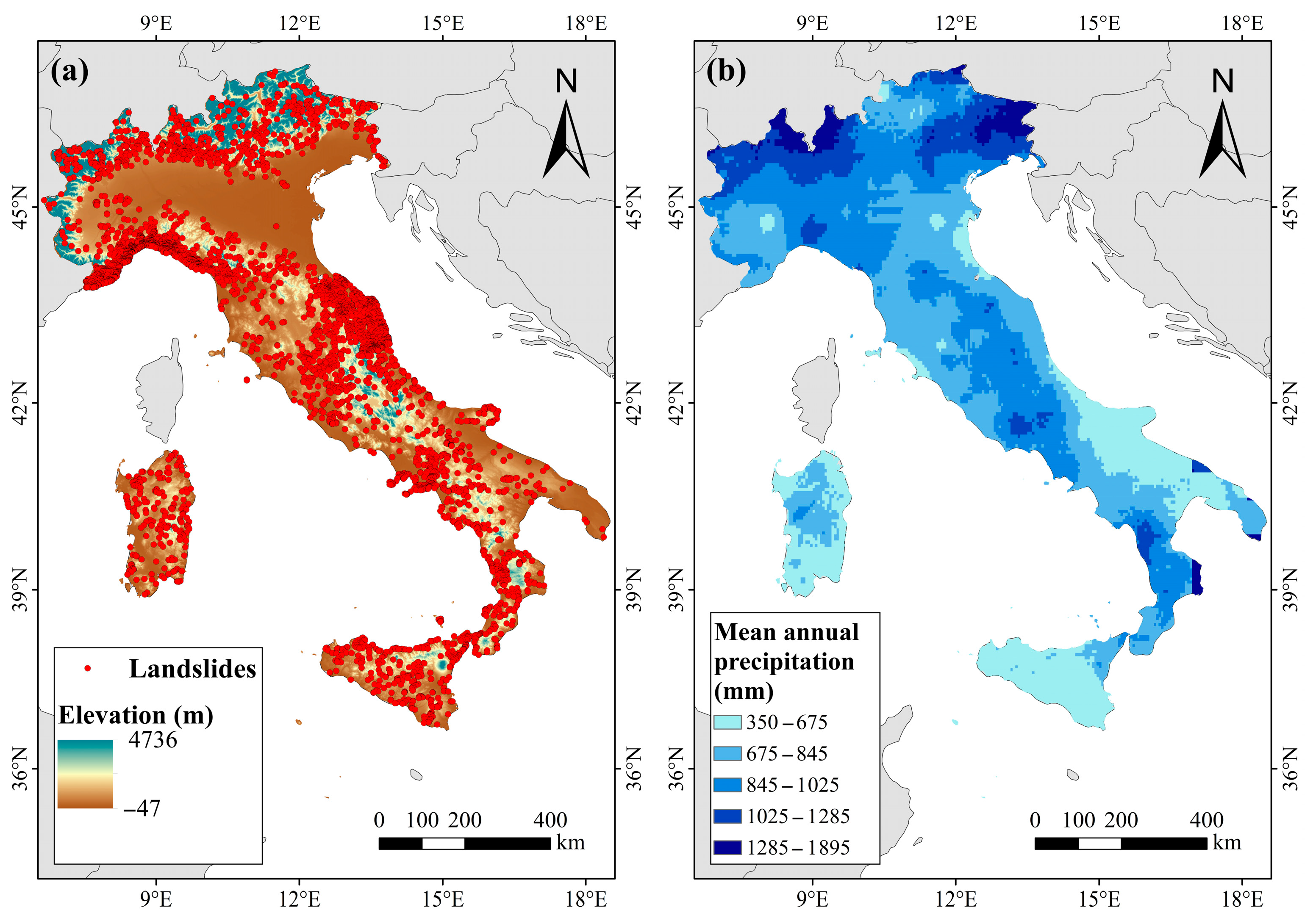
2.1. Study Area
2.2. Data
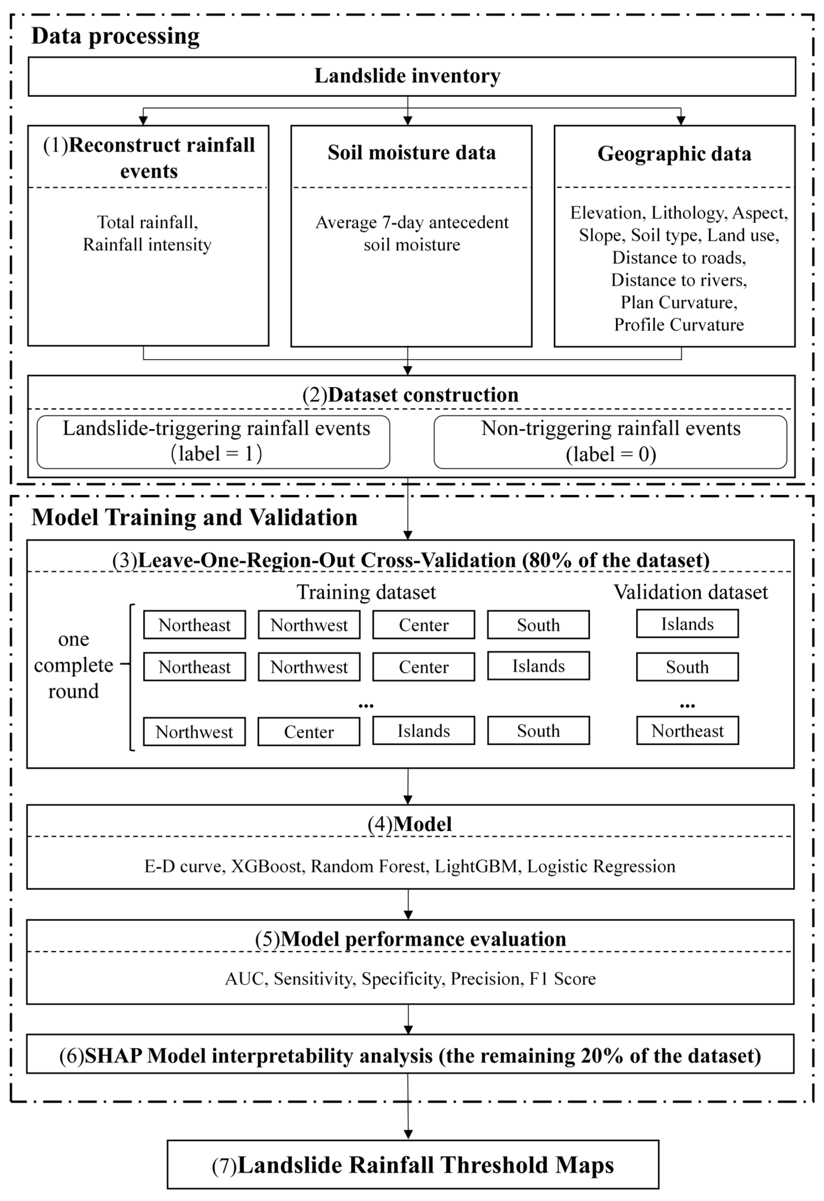
2.3. Methods
2.3.1. Rainfall Events
2.3.2. Rainfall Threshold Model
2.3.3. Machine Learning Models
2.3.4. Imbalanced Sample Processing
2.3.5. SHAP
2.3.6. Model Performance Evaluation
3. Results
3.1. Model Performance Comparison
3.2. SHAP Value Analysis
3.3. XGBoost Prediction Results
3.4. Spatial Analysis of Rainfall Thresholds for Landslide Triggering
4. Discussion
4.1. Machine Learning Model Performance
4.2. Landslide-Triggering Factors
4.3. Analysis of the Spatial Distribution of Rainfall Thresholds
4.4. Limitations and Future Perspectives
5. Conclusions
- (1)
- The XGBoost model achieved superior overall performance (AUC = 0.917 ± 0.026) with well-balanced sensitivity (0.792 ± 0.075) and specificity (0.812 ± 0.033), proving more suitable for modeling imbalanced datasets. The model significantly outperformed other machine learning approaches, thereby demonstrating its exceptional suitability for landslide modeling and early warning applications.
- (2)
- Total rainfall and rainfall intensity were the dominant triggering factors, far exceeding other factors in importance. SHAP analysis showed a pronounced increase in influence within the 30–50 mm range, with the maximum impact occurring beyond 50 mm. Rainfall intensity demonstrated critical thresholds above 21.5 mm/day, with peak influence beyond 47.9 mm/day. Among static environmental factors, elevation showed an inverse relationship with landslide probability, while proximity to rivers exhibited distance-dependent effects, with higher risk within 1500 m of waterways.
- (3)
- Regional differences in landslide-triggering rainfall thresholds were observed across Italy. Areas characterized by gentler terrain (slopes < 25°), such as Marche, Tuscany, and parts of Emilia-Romagna, along with moderate-rainfall regions including central Apennine areas and the Po Valley regions, demonstrated higher rainfall thresholds with values greater than 42 mm and 53 mm at 50% and 70% probability levels, respectively. In contrast, steeper slopes (>35°) found in regions such as Liguria, Umbria, and southern Calabria showed lower rainfall thresholds of less than 34 mm and 48 mm at the two probability levels, respectively. At the 90% probability level, thresholds universally increased, and regional disparities diminished.
Supplementary Materials
Author Contributions
Funding
Institutional Review Board Statement
Informed Consent Statement
Data Availability Statement
Acknowledgments
Conflicts of Interest
References
- Sidle, R.C.; Bogaard, T.A. Dynamic earth system and ecological controls of rainfall-initiated landslides. Earth-Sci. Rev. 2016, 159, 275–291. [Google Scholar] [CrossRef]
- Jiang, Z.; Fan, X.; Siva Subramanian, S.; Yang, F.; Tang, R.; Xu, Q.; Huang, R. Probabilistic rainfall thresholds for debris flows occurred after the Wenchuan earthquake using a Bayesian technique. Eng. Geol. 2021, 280, 105965. [Google Scholar] [CrossRef]
- Saito, H.; Nakayama, D.; Matsuyama, H. Relationship between the initiation of a shallow landslide and rainfall intensity—Duration thresholds in Japan. Geomorphology 2010, 118, 167–175. [Google Scholar] [CrossRef]
- Guzzetti, F. Landslide fatalities and the evaluation of landslide risk in Italy. Eng. Geol. 2000, 58, 89–107. [Google Scholar] [CrossRef]
- Gariano, S.L.; Guzzetti, F. Landslides in a changing climate. Earth-Sci. Rev. 2016, 162, 227–252. [Google Scholar] [CrossRef]
- Caine, N. The rainfall intensity-duration control of shallow landslides and debris flows. Geogr. Ann. A Phys. Geogr. 1980, 62, 23–27. [Google Scholar]
- Peruccacci, S.; Brunetti, M.T.; Luciani, S.; Vennari, C.; Guzzetti, F. Lithological and seasonal control on rainfall thresholds for the possible initiation of landslides in central Italy. Geomorphology 2012, 139, 79–90. [Google Scholar] [CrossRef]
- Liu, S.; Du, J.; Yin, K.; Zhou, C.; Huang, C.; Jiang, J.; Yu, J. Regional early warning model for rainfall induced landslide based on slope unit in Chongqing, China. Eng. Geol. 2024, 333, 107464. [Google Scholar] [CrossRef]
- Yang, H.Q.; Zhang, L. Bayesian back analysis of unsaturated hydraulic parameters for rainfall-induced slope failure: A review. Earth-Sci. Rev. 2024, 251, 104714. [Google Scholar] [CrossRef]
- Segoni, S.; Piciullo, L.; Gariano, S.L. A review of the recent literature on rainfall thresholds for landslide occurrence. Landslides 2018, 15, 1483–1501. [Google Scholar] [CrossRef]
- Vessia, G.; Di Curzio, D.; Chiaudani, A.; Rusi, S. Regional rainfall threshold maps drawn through multivariate geostatistical techniques for shallow landslide hazard zonation. Sci. Total Environ. 2020, 705, 135815. [Google Scholar] [CrossRef] [PubMed]
- Peruccacci, S.; Brunetti, M.T.; Gariano, S.L.; Melillo, M.; Rossi, M.; Guzzetti, F. Rainfall thresholds for possible landslide occurrence in Italy. Geomorphology 2017, 290, 39–57. [Google Scholar] [CrossRef]
- Crosta, G. Regionalization of rainfall thresholds: An aid to landslide hazard evaluation. Environ. Geol. 1998, 35, 131–145. [Google Scholar] [CrossRef]
- Segoni, S.; Rosi, A.; Rossi, G.; Catani, F.; Casagli, N. Analysing the relationship between rainfalls and landslides to define a mosaic of triggering thresholds for regional-scale warning systems. Nat. Hazards Earth Syst. Sci. 2014, 14, 2637–2648. [Google Scholar] [CrossRef]
- Segoni, S.; Lagomarsino, D.; Fanti, R.; Moretti, S.; Cassagli, N. Integration of rainfall thresholds and susceptibility maps in the Emilia Romagna (Italy) regional-scale landslide warning system. Landslides 2015, 12, 773–785. [Google Scholar] [CrossRef]
- Liu, Z.; Gilbert, G.; Cepeda, J.M.; Lysdahl, A.O.K.; Piciullo, L.; Hefre, H.; Lacasse, S. Modelling of shallow landslides with machine learning algorithms. Geosci. Front. 2021, 12, 385–393. [Google Scholar] [CrossRef]
- Merghadi, A.; Yunus, A.P.; Dou, J.; Whiteley, J.; ThaiPham, B.; Bui, D.T.; Avtar, R.; Abderrahmane, B. Machine learning methods for landslide susceptibility studies: A comparative overview of algorithm performance. Earth-Sci. Rev. 2020, 207, 103225. [Google Scholar] [CrossRef]
- Ng, C.W.W.; Yang, B.; Liu, Z.Q.; Kwan, J.S.H.; Chen, L. Spatiotemporal modelling of rainfall-induced landslides using machine learning. Landslides 2021, 18, 2499–2514. [Google Scholar] [CrossRef]
- Goetz, J.N.; Brenning, A.; Petschko, H.; Leopold, P. Evaluating machine learning and statistical prediction techniques for landslide susceptibility modeling. Comput. Geosci. 2015, 81, 1–11. [Google Scholar] [CrossRef]
- Lv, L.; Chen, T.; Dou, J.; Plaza, A. A hybrid ensemble-based deep-learning framework for landslide susceptibility mapping. Int. J. Appl. Earth Obs. Geoinf. 2022, 108, 102713. [Google Scholar] [CrossRef]
- Fang, Z.; Tanyas, H.; Gorum, T.; Dahal, A.; Wang, Y.; Lombardo, L. Speech-recognition in landslide predictive modelling: A case for a next generation early warning system. Environ. Model. Softw. 2023, 170, 105833. [Google Scholar] [CrossRef]
- Xiao, T.; Zhang, L.M. Data-driven landslide forecasting: Methods, data completeness, and real-time warning. Eng. Geol. 2023, 317, 107068. [Google Scholar] [CrossRef]
- Zhang, J.; Ma, X.; Zhang, J.; Sun, D.; Zhou, X.; Mi, C.; Wen, H. Insights into geospatial heterogeneity of landslide susceptibility based on the SHAP-XGBoost model. J. Environ. Manag. 2023, 332, 117357. [Google Scholar] [CrossRef]
- Hu, W.; Yang, Z.; Yang, J.; Li, Q.; Deng, J.; Zhao, S.; Cui, Y. Scale effects in landslide susceptibility assessment: Integrating slope unit division and SHAP-based interpretability in a typical river basin. Water 2025, 17, 1877. [Google Scholar] [CrossRef]
- Zhou, X.; Wen, H.; Li, Z.; Zhang, H.; Zhang, W. An interpretable model for the susceptibility of rainfall-induced shallow landslides based on SHAP and XGBoost. Geocarto Int. 2022, 37, 13419–13450. [Google Scholar] [CrossRef]
- Fantappiè, M.; L’Abate, G.; Schillaci, C.; Costantini, E.A. Digital soil mapping of Italy to map derived soil profiles with neural networks. Geoderma Reg. 2023, 32, e00619. [Google Scholar] [CrossRef]
- Peruccacci, S.; Gariano, S.L.; Melillo, M.; Solimano, M.; Guzzetti, F.; Brunetti, M.T. The ITAlian rainfall-induced LandslIdes CAtalogue, an extensive and accurate spatio-temporal catalogue of rainfall-induced landslides in Italy. Earth Syst. Sci. Data 2023, 15, 2863–2877. [Google Scholar] [CrossRef]
- Di Napoli, M.; Carotenuto, F.; Cevasco, A.; Confuorto, P.; Di Martire, D.; Firpo, M.; Pepe, G.; Raso, E.; Calcaterra, D. Machine learning ensemble modelling as a tool to improve landslide susceptibility mapping reliability. Landslides 2020, 17, 1897–1914. [Google Scholar] [CrossRef]
- Meena, S.R.; Puliero, S.; Bhuyan, K.; Floris, M.; Catani, F. Assessing the importance of conditioning factor selection in landslide susceptibility for the province of Belluno (region of Veneto, northeastern Italy). Nat. Hazards Earth Syst. Sci. 2022, 22, 1395–1417. [Google Scholar] [CrossRef]
- Mehrabi, M. Landslide susceptibility zonation using statistical and machine learning approaches in Northern Lecco, Italy. Nat. Hazards 2021, 108, 1–37. [Google Scholar] [CrossRef]
- Panday, S.; Dong, J.J. Topographical features of rainfall-triggered landslides in Mon State, Myanmar, August 2019: Spatial distribution heterogeneity and uncommon large relative heights. Landslides 2021, 18, 3875–3889. [Google Scholar] [CrossRef]
- Marin, R.J. Physically based and distributed rainfall intensity and duration thresholds for shallow landslides. Landslides 2020, 17, 2907–2917. [Google Scholar] [CrossRef]
- Ávila, F.F.; Alvalá, R.C.; Mendes, R.M.; Amore, D.J. The influence of land use/land cover variability and rainfall intensity in triggering landslides: A back-analysis study via physically based models. Nat. Hazards 2021, 105, 1139–1161. [Google Scholar] [CrossRef]
- Guzzetti, F.; Melillo, M.; Mondini, A.C. Landslide predictions through combined rainfall threshold models. Landslides 2025, 22, 137–147. [Google Scholar] [CrossRef]
- Segoni, S.; Tofani, V.; Rosi, A.; Catani, F.; Casagli, N. Combination of rainfall thresholds and susceptibility maps for dynamic landslide hazard assessment at regional scale. Front. Earth Sci. 2018, 6, 85. [Google Scholar] [CrossRef]
- Funk, C.; Peterson, P.; Landsfeld, M.; Pedreros, D.; Verdin, J.; Shukla, S.; Husak, G.; Rowland, J.; Harrison, L.; Hoell, A.; et al. The climate hazards infrared precipitation with stations—A new environmental record for monitoring extremes. Sci. Data 2015, 2, 1–21. [Google Scholar] [CrossRef]
- Wicki, A.; Lehmann, P.; Hauck, C.; Seneviratne, S.I.; Waldner, P.; Stähli, M. Assessing the potential of soil moisture measurements for regional landslide early warning. Landslides 2020, 17, 1881–1896. [Google Scholar] [CrossRef]
- Marino, P.; Peres, D.; Cancelliere, A.; Greco, R.; Bogaard, T. Soil moisture information can improve shallow landslide forecasting using the hydrometeorological threshold approach. Landslides 2020, 17, 2041–2054. [Google Scholar] [CrossRef]
- Orth, R.; Weber, U.; Park, S.K. High-resolution European daily soil moisture derived with machine learning (2003–2020). Sci. Data 2022, 9, 1–13. [Google Scholar] [CrossRef]
- Mondini, A.C.; Guzzetti, F.; Melillo, M. Deep learning forecast of rainfall-induced shallow landslides. Nat. Commun. 2023, 14, 2466. [Google Scholar] [CrossRef]
- Brunetti, M.T.; Peruccacci, S.; Rossi, M.; Luciani, S.; Valigi, D.; Guzzetti, F. Rainfall thresholds for the possible occur-rence of landslides in Italy. Nat. Hazards Earth Syst. Sci. 2010, 10, 447–458. [Google Scholar] [CrossRef]
- Dal Seno, N.; Evangelista, D.; Piccolomini, E.; Berti, M. Comparative analysis of conventional and machine learning techniques for rainfall threshold evaluation under complex geological conditions. Landslides 2024, 21, 2893–2911. [Google Scholar] [CrossRef]
- Gariano, S.L.; Sarkar, R.; Dikshit, A.; Dorji, K.; Brunetti, M.T.; Peruccacci, S.; Melillo, M. Automatic calculation of rainfall thresholds for landslide occurrence in Chukha Dzongkhag, Bhutan. Bull. Eng. Geol. Environ. 2019, 78, 4325–4332. [Google Scholar] [CrossRef]
- Lollino, G.; Arattano, M.; Allasia, P.; Giordan, D. Time response of a landslide to meteorological events. Nat. Hazards Earth Syst. Sci. 2006, 6, 179–184. [Google Scholar] [CrossRef]
- Chen, T.; Guestrin, C. XGBoost: A Scalable Tree Boosting System. In Proceedings of the 22nd ACM SIGKDD International Conference on Knowledge Discovery and Data Mining, San Francisco, CA, USA, 13–17 August 2016; pp. 785–794. [Google Scholar]
- Breiman, L. Random forests. Mach. Learn. 2001, 45, 5–32. [Google Scholar] [CrossRef]
- Ke, G.; Meng, Q.; Finley, T.; Wang, T.; Chen, W.; Ma, W.; Liu, T.Y. Lightgbm: A highly efficient gradient boosting decision tree. Adv. Neural Inf. Process. Syst. 2017, 30, 3147–3155. [Google Scholar]
- Hosmer, D.W., Jr.; Lemeshow, S.; Sturdivant, R.X. Applied Logistic Regression; John Wiley & Sons: Hoboken, NJ, USA, 2013. [Google Scholar]
- Thompson, S.K. Sampling; John Wiley & Sons: Hoboken, NJ, USA, 2012. [Google Scholar]
- Stone, M. Cross-validatory choice and assessment of statistical predictions. J. R. Stat. Soc. B Stat. Methodol. 1974, 36, 111–133. [Google Scholar] [CrossRef]
- Chawla, N.V.; Bowyer, K.W.; Hall, L.O.; Kegelmeyer, W.P. SMOTE: Synthetic minority over-sampling technique. J. Artif. Intell. Res. 2002, 16, 321–357. [Google Scholar] [CrossRef]
- Kuhn, H.W. (Ed.) Classics in Game Theory; Princeton University Press: Princeton, NJ, USA, 1997. [Google Scholar]
- Lundberg, S.M.; Lee, S.I. A unified approach to interpreting model predictions. Adv. Neural Inf. Process. Syst. 2017, 30, 4768–4777. [Google Scholar]
- He, H.; Garcia, E.A. Learning from imbalanced data. IEEE Trans. Knowl. Data Eng. 2009, 21, 1263–1284. [Google Scholar] [CrossRef]
- Bishop, C.M.; Nasrabadi, N.M. Pattern Recognition and Machine Learning; Springer: New York, NY, USA, 2006. [Google Scholar]
- Fawcett, T. An introduction to ROC analysis. Pattern Recognit. Lett. 2006, 27, 861–874. [Google Scholar] [CrossRef]
- Hanley, J.A.; McNeil, B.J. The meaning and use of the area under a receiver operating characteristic (ROC) curve. Radiology 1982, 143, 29–36. [Google Scholar] [CrossRef]
- Kutlug Sahin, E.; Colkesen, I. Performance analysis of advanced decision tree-based ensemble learning algorithms for landslide susceptibility mapping. Geocarto Int. 2021, 36, 1253–1275. [Google Scholar] [CrossRef]
- Iverson, R.M. Landslide triggering by rain infiltration. Water Resour. Res. 2000, 36, 1897–1910. [Google Scholar] [CrossRef]
- Guzzetti, F.; Peruccacci, S.; Rossi, M.; Stark, C.P. The rainfall intensity–duration control of shallow landslides and debris flows: An update. Landslides 2008, 5, 3–17. [Google Scholar] [CrossRef]
- Guzzetti, F.; Carrara, A.; Cardinali, M.; Reichenbach, P. Landslide hazard evaluation: A review of current techniques and their application in a multi-scale study, Central Italy. Geomorphology 1999, 31, 181–216. [Google Scholar] [CrossRef]
- Azarafza, M.; Azarafza, M.; Akgün, H.; Atkinson, P.M.; Derakhshani, R. Deep learning-based landslide susceptibility mapping. Sci. Rep. 2021, 11, 24112. [Google Scholar] [CrossRef]
- Kumar, C.; Walton, G.; Santi, P.; Luza, C. An ensemble approach of feature selection and machine learning models for regional landslide susceptibility mapping in the arid mountainous terrain of Southern Peru. Remote Sens. 2023, 15, 1376. [Google Scholar] [CrossRef]
- Gariano, S.L.; Brunetti, M.; Iovine, G.; Melillo, M.; Peruccacci, S.; Terranova, O.; Vennari, C.; Huzzetti, F. Calibration and validation of rainfall thresholds for shallow landslide forecasting in Sicily, southern Italy. Geomorphology 2015, 228, 653–665. [Google Scholar] [CrossRef]
- Melillo, M.; Brunetti, M.T.; Peruccacci, S.; Gariano, S.L.; Guzzetti, F. Rainfall thresholds for the possible landslide occurrence in Sicily (Southern Italy) based on the automatic reconstruction of rainfall events. Landslides 2016, 13, 165–172. [Google Scholar] [CrossRef]


| Factors | Scale/Resolution | Source |
|---|---|---|
| Elevation | 10 m | https://tinitaly.pi.ingv.it/ (accessed on 10 November 2024) |
| Slope | 10 m | https://tinitaly.pi.ingv.it/ (accessed on 10 November 2024) |
| Aspect | 10 m | https://tinitaly.pi.ingv.it/ (accessed on 10 November 2024) |
| Plan curvature | 10 m | https://tinitaly.pi.ingv.it/ (accessed on 10 November 2024) |
| Profile curvature | 10 m | https://tinitaly.pi.ingv.it/ (accessed on 10 November 2024) |
| Lithology | 1:100,000 | https://doi.org/10.1594/PANGAEA.935673 (accessed on 26 November 2024) |
| Soil type | 1000 m | https://esdac.jrc.ec.europa.eu (accessed on 26 November 2024) |
| Land use | 30 m | https://zenodo.org/records/3986872 (accessed on 26 November 2024) |
| Distance to roads | 100 m | https://www.openstreetmap.org/ (accessed on 29 November 2024) |
| Distance to rivers | 100 m | https://www.openstreetmap.org/ (accessed on 29 November 2024) |
| Factors | Code | Description |
|---|---|---|
| Lithology | Al | Alluvial, lacustrine, swamp and marine deposits. Eluvial and colluvial deposits |
| Nsr | Non-schistose metamorphic rocks | |
| Cr | Carbonate rocks | |
| Ssr | Siliciclastic sedimentary rocks | |
| Ucr | Unconsolidated clastic rock | |
| M | Marlstone | |
| Ccr | Consolidated clastic rocks | |
| Ir | Intrusive rocks | |
| Sr | Schistose metamorphic rocks | |
| Pr | Pyroclastic rocks | |
| Lb | Lavas and basalts | |
| E | Evaporite | |
| B | Beaches and coastal deposits | |
| CM | Chaotic—mélange | |
| Ad | Anthropogenic deposits | |
| SM | Mixed sedimentary rocks | |
| Gd | Glacial drift | |
| Mw | Mass wasting material | |
| Li | Lakes and Ice | |
| Soil Type | AN | Andosol |
| CM | Cambisol | |
| FL | Fluvisol | |
| GL | Gleysol | |
| HS | Histosol | |
| LP | Leptosol | |
| LV | Luvisol | |
| PZ | Podzol | |
| RG | Regosol | |
| VR | Vertisol | |
| Land Use | 1 | Rain-fed cropland |
| 2 | Herbaceous cover | |
| 3 | Tree or shrub cover (orchard) | |
| 4 | Irrigated cropland | |
| 5 | Evergreen broadleaved forest | |
| 6 | Closed deciduous broadleaved forest | |
| 7 | Open deciduous broadleaved forest | |
| 8 | Closed evergreen needleleaved forest | |
| 9 | Open evergreen needleleaved forest | |
| 10 | Mixed-leaf forest | |
| 11 | Shrubland | |
| 12 | Grassland | |
| 13 | Sparse vegetation | |
| 14 | Sparse herbaceous cover | |
| 15 | Wetlands | |
| 16 | Impervious surfaces | |
| 17 | Bare areas | |
| 18 | Consolidated bare areas | |
| 19 | Unconsolidated bare areas | |
| 20 | Water body | |
| 21 | Permanent ice and snow |
| Model | Parameter | Search Space |
|---|---|---|
| XGBoost | n_estimators | [50, 100, 200, 300] |
| max_depth | [5, 10, 20, 40] | |
| learning_rate | [0.01, 0.1, 0.2, 0.3] | |
| subsample | [0.8, 0.9, 1.0] | |
| colsample_bytree | [0.8, 0.9, 1.0] | |
| RF | n_estimators | [50, 100, 200, 300] |
| max_depth | [5, 10, 20, 40] | |
| min_samples_split | [2, 5, 10] | |
| min_samples_leaf | [1, 2, 4] | |
| max_features | [‘sqrt’, ‘log2’, None] | |
| LightGBM | n_estimators | [50, 100, 200, 300] |
| max_depth | [5, 10, 20, 40] | |
| learning_rate | [0.01, 0.1, 0.2, 0.3] | |
| subsample | [0.8, 0.9, 1.0] | |
| colsample_bytree | [0.8, 0.9, 1.0] | |
| LR | C | [0.01, 0.1, 1, 10, 100] |
| penalty | [‘l1’, ‘l2’, ‘elasticnet’] | |
| solver | [‘liblinear’, ‘lbfgs’, ‘saga’] | |
| max_iter | [100, 200, 500, 1000] |
| Macro-Region | Region | Training and Validation Set | Test Set | ||
|---|---|---|---|---|---|
| Positive Sample | Negative Sample | Positive Sample | Negative Sample | ||
| Northwest | Aosta Valley, Piedmont, Liguria, Lombardy | 1501 | 15,010 | 375 | 3750 |
| Center | Tuscany, Umbria, Marche, Lazio | 1406 | 14,060 | 352 | 3520 |
| South | Abruzzo, Molise, Campania, Apulia (Puglia), Basilicata, Calabria | 694 | 6940 | 173 | 1730 |
| Islands | Sicily, Sardinia | 471 | 4710 | 117 | 1170 |
| Northeast | Trentino-Alto Adige/South Tyrol, Veneto, Friuli Venezia Giulia, Emilia-Romagna | 340 | 3400 | 85 | 850 |
| Model | AUC | Sensitivity | Specificity | F1 Score | Precision | Optimized Hyperparameter |
|---|---|---|---|---|---|---|
| XGBoost | 0.917 ± 0.026 | 0.792 ± 0.075 | 0.812 ± 0.033 | 0.731 ± 0.037 | 0.681 ± 0.032 | n_estimators = 200, max_depth = 40, learning_rate = 0.01, subsample = 0.8, colsample_bytree = 0.8 |
| Random Forest | 0.916 ± 0.026 | 0.696 ± 0.134 | 0.906 ± 0.043 | 0.736 ± 0.063 | 0.795 ± 0.059 | n_estimators = 200, max_depth = 40, min_samples_split = 5, min_samples_leaf = 2, max_features = ‘sqrt’ |
| LightGBM | 0.917 ± 0.026 | 0.670 ± 0.111 | 0.930 ± 0.035 | 0.739 ± 0.074 | 0.831 ± 0.060 | n_estimators = 300, max_depth = 20, learning_rate = 0.01, subsample = 0.8, colsample_bytree = 0.8 |
| Logistic Regression | 0.813 ± 0.016 | 0.699 ± 0.085 | 0.747 ± 0.137 | 0.637 ± 0.032 | 0.597 ± 0.099 | C = 0.1, penalty = ‘elasticnet’, solver = ‘saga’, max_iter = 500 |
| E-D curve | 0.903 ± 0.032 | 1.000 ± 0.000 | 0.219 ± 0.034 | 0.565 ± 0.012 | 0.394 ± 0.012 | - |
Disclaimer/Publisher’s Note: The statements, opinions and data contained in all publications are solely those of the individual author(s) and contributor(s) and not of MDPI and/or the editor(s). MDPI and/or the editor(s) disclaim responsibility for any injury to people or property resulting from any ideas, methods, instructions or products referred to in the content. |
© 2025 by the authors. Licensee MDPI, Basel, Switzerland. This article is an open access article distributed under the terms and conditions of the Creative Commons Attribution (CC BY) license (https://creativecommons.org/licenses/by/4.0/).
Share and Cite
Shao, X.; Yan, W.; Yan, C.; Zhao, W.; Wang, Y.; Shi, X.; Dong, H.; Li, T.; Yu, J.; Zuo, P.; et al. Explainable Machine Learning for Mapping Rainfall-Induced Landslide Thresholds in Italy. Appl. Sci. 2025, 15, 7937. https://doi.org/10.3390/app15147937
Shao X, Yan W, Yan C, Zhao W, Wang Y, Shi X, Dong H, Li T, Yu J, Zuo P, et al. Explainable Machine Learning for Mapping Rainfall-Induced Landslide Thresholds in Italy. Applied Sciences. 2025; 15(14):7937. https://doi.org/10.3390/app15147937
Chicago/Turabian StyleShao, Xiangyu, Wenjun Yan, Chaoying Yan, Wen Zhao, Yixuan Wang, Xia Shi, Hongchang Dong, Tianjiang Li, Junpo Yu, Peng Zuo, and et al. 2025. "Explainable Machine Learning for Mapping Rainfall-Induced Landslide Thresholds in Italy" Applied Sciences 15, no. 14: 7937. https://doi.org/10.3390/app15147937
APA StyleShao, X., Yan, W., Yan, C., Zhao, W., Wang, Y., Shi, X., Dong, H., Li, T., Yu, J., Zuo, P., Zhou, Z., & Jin, J. (2025). Explainable Machine Learning for Mapping Rainfall-Induced Landslide Thresholds in Italy. Applied Sciences, 15(14), 7937. https://doi.org/10.3390/app15147937