Deep Learning-Based Crack Detection on Cultural Heritage Surfaces

Abstract

This study employs a deep learning-based object detection model, GoogleNet, to identify cracks in cultural heritage images. Subsequently, a semantic segmentation model, SegNet, is utilized to determine the location and extent of the cracks. To establish a scale ratio between image pixels and real-world dimensions, a parallel laser-based measurement approach is applied, enabling precise crack length calculations. The results indicate that the percentage error between crack lengths estimated using deep learning and those measured with a caliper is approximately 3%, demonstrating the feasibility and reliability of the proposed method. Additionally, the study examines the impact of iteration count, image quantity, and image category on the performance of GoogleNet and SegNet. While increasing the number of iterations significantly improves the models’ learning performance in the early stages, excessive iterations lead to overfitting. The optimal performance for GoogleNet was achieved at 75 iterations, whereas SegNet reached its best performance after 45,000 iterations. Similarly, while expanding the training dataset enhances model generalization, an excessive number of images may also contribute to overfitting. GoogleNet exhibited optimal performance with a training set of 66 images, while SegNet achieved the best segmentation accuracy when trained with 300 images. Furthermore, the study investigates the effect of different crack image categories by classifying datasets into four groups: general cracks, plain wall cracks, mottled wall cracks, and brick wall cracks. The findings reveal that training GoogleNet and SegNet with general crack images yielded the highest model performance, whereas training with a single crack category substantially reduced generalization capability.

1. Introduction

Historic buildings constitute invaluable cultural assets, embodying significant historical and artistic heritage. However, these structures are particularly susceptible to deterioration resulting from environmental influences, climate change, and human activity. Among various forms of structural damage, crack formation is especially prevalent, posing substantial threats to structural integrity and diminishing both cultural and historical value [1]. Accordingly, accurate detection and timely remediation of cracks are essential components of heritage conservation efforts [2]. Heritage conservation encompasses a range of approaches, including preservation, rehabilitation, restoration, and reconstruction, all of which prioritize the retention of original materials and respect for historical context. The effectiveness of conservation efforts is further enhanced by the implementation of preventive strategies, routine maintenance, and active community participation [3].

Conventional crack detection methods predominantly rely on expert visual inspections, often supported by manual measurements to determine crack dimensions and distribution. Although these methods are straightforward, they are inefficient for large-scale surveys and prone to subjectivity and human error. The measurement discrepancies among different inspectors have been reported to exceed 8% [4]. In contrast, the deviation between crack measurements obtained using deep learning-based methods and those acquired manually with measuring tools ranges from 0.4% to 5% [5]. Peta et al. [6] employed a fractal theory-based approach to analyze heritage surfaces. This method effectively distinguishes surface features, such as impressions, cracks, and wear, at specific observational scales. To improve accuracy and efficiency, image processing techniques such as edge detection and thresholding have been employed. However, these methods often underperform in conditions with uneven lighting or complex backgrounds, necessitating manual adjustment for image preprocessing and parameter tuning [7,8].

Recent advancements in deep learning, particularly in Convolutional Neural Networks (CNNs), have significantly improved crack detection performance [9,10]. CNN-based models, widely adopted in computer vision, can be broadly categorized into image classification, object detection, semantic segmentation, and instance segmentation models.

Image classification models such as AlexNet [11], GoogleNet [12], and ResNet [13] are designed to categorize an entire image. In contrast, object detection models, including Faster R-CNN [14], YOLO [15], and SSD [16], identify both the location and class of multiple targets within an image. Semantic segmentation models, such as FCN [17], U-Net [18], and SegNet [19], assign a category to each pixel, providing fine-grained analysis. Instance segmentation models, including Mask R-CNN [20] and later versions of YOLO [21], combine object detection and semantic segmentation to distinguish individual objects along with their pixel-level boundaries. While functionally related, classification models assign a single label per image, whereas detection and segmentation models identify multiple regions or features.

Numerous studies have explored the application of deep learning models in crack detection. Object detection models are frequently used for rapid localization of cracks [22,23,24,25,26], while semantic segmentation models enable detailed pixel-level analysis, facilitating the measurement of crack morphology [27,28,29,30,31]. However, relatively few studies employ a combination of different model types. One contributing factor is the emergence of instance segmentation models, which already integrate detection and segmentation capabilities and have been applied to crack measurement [32,33,34]. Nonetheless, such models typically require high-performance computing resources for training and optimal inference.

To address these limitations, this study presents an integrated deep learning framework that combines the image classification model GoogleNet with the semantic segmentation model SegNet for crack detection in historic buildings. GoogleNet is used to perform global feature extraction and image-level classification [35,36], while SegNet facilitates pixel-level segmentation of crack boundaries and patterns. To convert image data into real-world measurements, a dual-laser system is employed for pixel-to-length calibration.

By integrating the classification capabilities of GoogleNet with the segmentation precision of SegNet, this study presents a practical and efficient end-to-end workflow for crack detection, delineation, and quantification. Although the architecture is based on established deep learning models, the novelty of this work lies in its integration within a unified framework specifically designed for heritage crack analysis. The proposed approach combines image classification for preliminary screening with semantic segmentation for detailed mapping, enhanced by a field-based dual-laser calibration technique.

The key contributions of this study are as follows:

• A two-stage workflow is introduced, wherein image classification is first employed to identify images containing potential cracks, followed by semantic segmentation to delineate crack regions. This approach offers a lower computational cost compared to more complex instance segmentation models.
• By integrating segmentation outputs with a simple yet effective field-based tool (parallel lasers), the method facilitates accurate estimation of crack lengths.
• The proposed framework demonstrates strong adaptability to varying lighting conditions and background textures typical of heritage surfaces. Its lightweight design also enables potential deployment on portable platforms.

Overall, this study presents an effective interdisciplinary methodology that bridges deep learning techniques with heritage conservation practices, offering practical applications for digital documentation, preservation, and structural monitoring of historic buildings.

2. Materials and Methods

2.1. Image Collection

Image collection is a critical step in the research process, as it significantly influences the efficiency and reliability of subsequent analyses. In this study, images were primarily captured using an iPhone 14 (Apple Inc., Cupertino, CA, USA), equipped with a high-resolution 12-megapixel main camera, enabling the detailed documentation of crack features. A total of 65 crack images from cultural heritage sites in Miaoli County were collected, representing three distinct types of cracks: brick wall cracks, mottled wall cracks, and plain wall cracks.

The first category, brick wall cracks, consisted of 21 images. These cracks are commonly found in historical buildings. According to [37], brick structures, composed of materials such as bricks, stones, and limestone bound by mortar, are among the most prevalent architectural forms worldwide and hold substantial cultural heritage significance. Regular maintenance of brick structures is essential to preserve their structural integrity and historical value.

The second category, mottled wall cracks, comprised 22 images. These cracks typically appear as network-like patterns within flaking areas of the wall, often resulting from moisture exposure or chemical erosion. The third category, plain wall cracks, included 22 images. These cracks, often forming as vertical linear fractures, are usually caused by uneven structural load distribution or seismic activity.

In addition to crack images, 50 non-crack images were collected, featuring corridors, floors, and walls without visible cracks. These non-crack images served as control samples to enhance the deep learning model’s training completeness by facilitating contrast-based learning. The inclusion of contrast samples aims to enhance the model’s ability to distinguish cracks from non-cracks, reduce false positive rates, improve adaptability across diverse environments, optimize the training process, and bolster generalization capabilities. Furthermore, it minimizes the risk of overfitting, increases reliability, and ensures the model’s effectiveness in real-world applications.

Due to the limited number of images sourced from cultural heritage sites in Miaoli County, it was challenging to achieve satisfactory performance using large-scale deep learning models such as Mask R-CNN or Fast R-CNN. Consequently, this study employs a relatively lightweight architecture by integrating GoogleNet with SegNet. The proposed framework first identifies whether an image contains cracks, then performs crack segmentation, and ultimately calculates the crack length. A total of 21 images of brick wall cracks, 22 images of mottled wall cracks, and 22 images of plain wall cracks were selected to ensure balanced performance across the three crack types in subsequent analyses and applications.

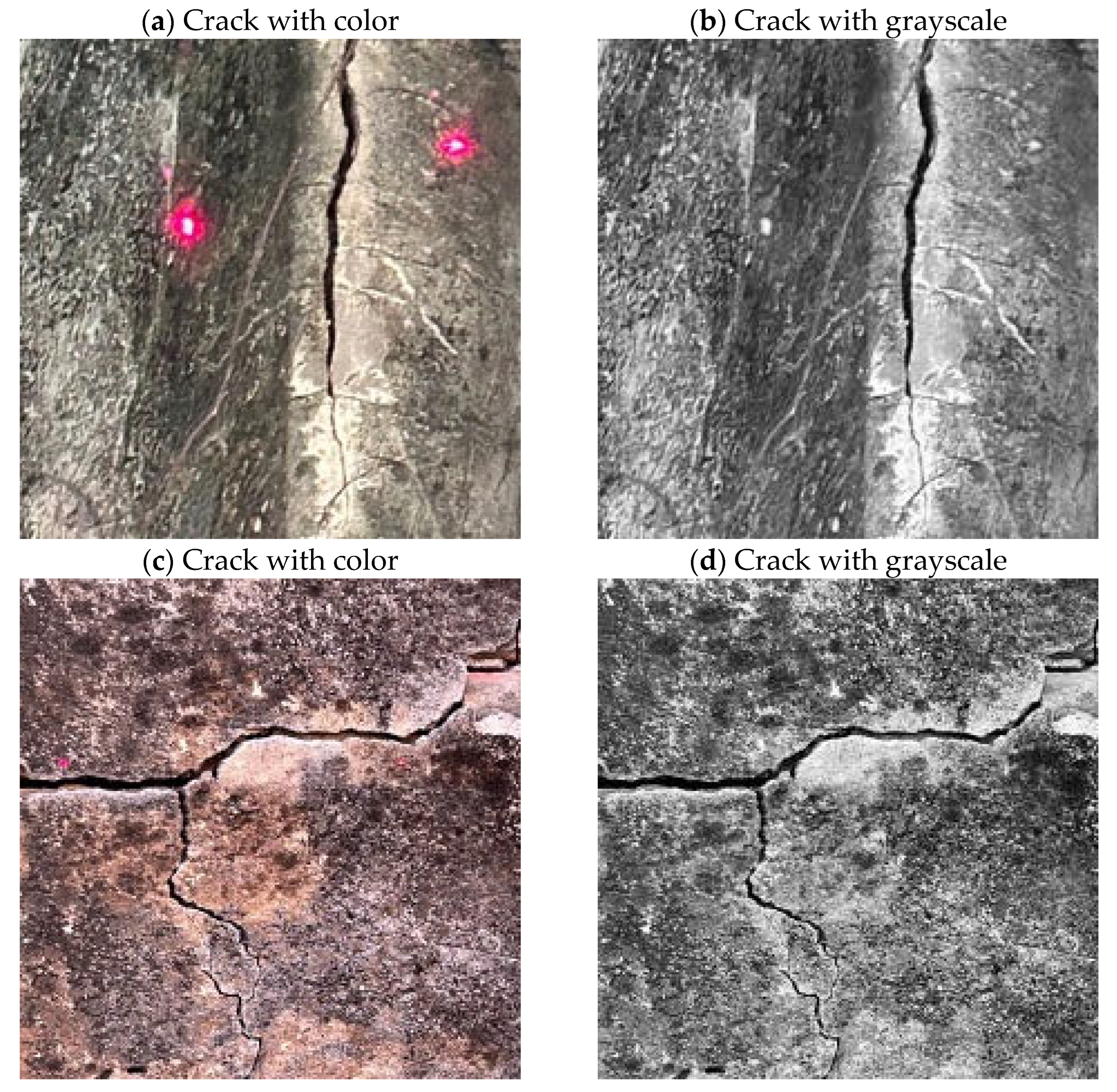
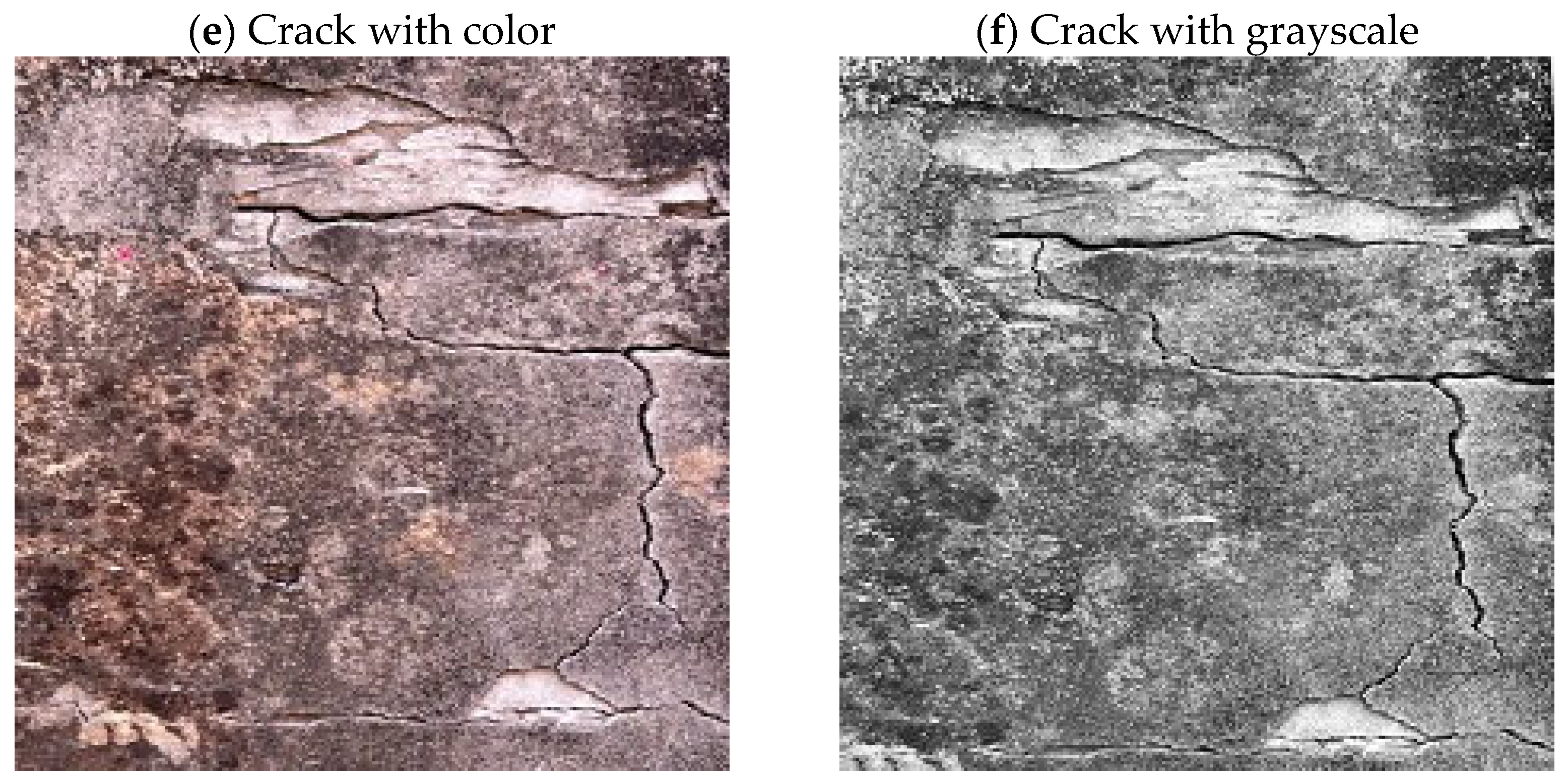
2.2. Image Preprocessing

Image preprocessing is a fundamental component of deep learning applications in image analysis. The first preprocessing step in this study involved converting color images to grayscale. Since color images consist of red, green, and blue channels, converting them to grayscale, which contains only a single channel, significantly reduces data volume and computational demand. This reduction is especially beneficial in resource-constrained environments, as it enhances both training and inference efficiency. As highlighted by [37], grayscale conversion improves numerical analysis reliability and enhances geometric representation in structural analysis. Simple preprocessing techniques, such as contrast enhancement, facilitate the extraction of crack features. Golding et al. [38] demonstrated that color-independent features are crucial for crack detection in deep learning, suggesting that grayscale images can enhance model performance. In this study, grayscale conversion was applied to help models focus on essential crack features. Figure 1 illustrates crack patterns in images before and after grayscale conversion.

The second preprocessing step involved standardizing image dimensions, a crucial requirement for deep learning models, as they typically require fixed-size input images. Variability in input dimensions can hinder effective model training and negatively impact generalization and accuracy. Golding et al. [38] demonstrated that image resizing and standardization can enhance analytical efficiency while improving accuracy, precision, and F1-score. Although numerous studies have reported that higher image resolution generally yields more accurate results [39,40,41], the processing capacity of most deep learning models is constrained by hardware limitations, typically restricting input image sizes to below 500,000 pixels. In the present study, all images were uniformly resized to 224 × 224 pixels. As such, the resolution offered by most commercially available smartphone cameras is sufficient to fulfill the image requirements for the proposed methodology.

The third preprocessing step was image annotation, which entails accurately labeling specific objects or regions within an image by defining object boundaries or assigning categorical labels. These annotations provide deep learning models with essential ground truth data, enabling accurate identification and classification of new image data. Qiu et al. [42] demonstrated that marking boundary boxes in crack images improves model accuracy and detection speed. In this study, the Image Labeler tool in MATLAB R2022a was used for image annotation.

The final preprocessing step involved data augmentation (DA), which applies transformations such as flipping, rotation, and translation to increase dataset variability. This process not only enhances image quality but also exposes the model to a broader range of scenarios, reducing the risk of overfitting. Data augmentation strengthens the model’s adaptability to dynamic environments and broadens its experiential scope, allowing for better generalization to new or unfamiliar contexts. Additionally, it reduces reliance on specific image characteristics, thereby further improving generalization. In this study, the imageDataAugmenter function in MATLAB was employed to introduce a series of random transformations to the input images.

2.3. Deep Learning Models

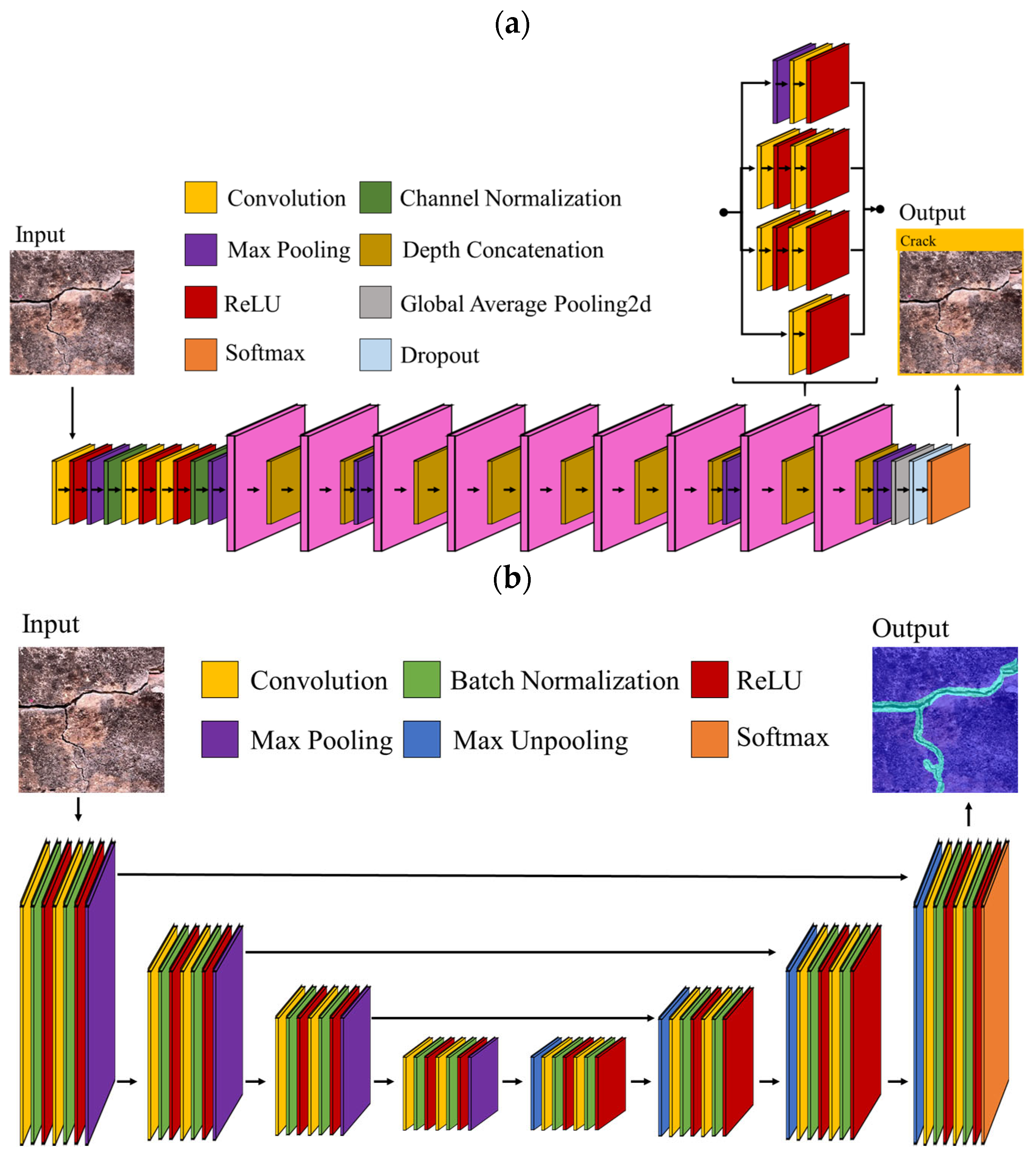
2.3.1. GoogleNet Model

GoogleNet, introduced by researchers at Google in 2014, was inspired by the Network in Network (NiN) architecture proposed by [43]. It secured first place in the ImageNet Large Scale Visual Recognition Challenge (ILSVRC) image classification competition, surpassing VGGNet [44] in accuracy. Evolving from earlier architectures such as LeNet-5, GoogleNet enhanced the capability of convolutional neural networks (CNNs) to address complex image classification tasks, including datasets such as MNIST, CIFAR, and ImageNet. Key advancements included increasing network depth and layer size, integrating dropout techniques to mitigate overfitting, and incorporating max-pooling layers to enhance feature extraction, despite the potential loss of spatial information. These improvements rendered GoogleNet effective not only in image classification but also in related tasks such as localization, object detection, and face recognition.

A notable innovation of GoogleNet was the introduction of the inception module, which facilitated multi-scale feature extraction by integrating convolution operations of varying kernel sizes within the same layer. This design reduced the number of parameters (weights and biases) while improving the network’s representational capacity. Szegedy et al. [12] further refined this approach by employing 1 × 1 convolutions for dimensionality reduction, enabling deeper and wider architectures without a proportional increase in computational complexity. This strategy, known as the bottleneck design, contributed to the development of highly efficient deep learning models capable of learning intricate feature representations.

The GoogleNet architecture comprises 22 layers, or 27 layers when pooling layers are included. It processes RGB images with a resolution of 224 × 224 pixels, leveraging 1 × 1 convolutions prior to 3 × 3 and 5 × 5 convolutions to optimize dimensionality reduction and computational efficiency (Figure 2a). The rectified linear unit (ReLU) activation function is utilized throughout the network. During training, auxiliary classifiers are incorporated into intermediate layers to address the gradient vanishing problem and provide additional regularization.

2.3.2. SegNet Model

Badrinarayanan et al. [19] introduced Fully Convolutional Networks (FCNs) for semantic segmentation, a deep learning framework designed for pixel-level image annotation. SegNet, an FCN-based model, employs an encoder–decoder structure wherein the encoder extracts hierarchical features, and the decoder reconstructs these features to match the original image resolution for precise pixel-level classification. The encoder is derived from the VGG16 architecture proposed by [45], incorporating its first 13 convolutional layers while omitting fully connected layers. This modification enhances the efficiency of semantic segmentation by reducing computational complexity.

A distinguishing feature of SegNet is its use of max-pooling indices from the encoder to guide non-linear upsampling in the decoder. This eliminates the need for learning additional upsampling techniques, thereby improving memory efficiency, reducing model size, and lowering the number of parameters from 134 million to 14.7 million while accelerating convergence. By leveraging broader contextual information, SegNet enhances accuracy and optimizes memory utilization and computational efficiency. Figure 2b illustrates the architecture of the SegNet model.

SegNet demonstrates high efficiency in processing images and generating accurate, coherent predictions across various scene depths and contexts. Through its encoder–decoder structure, it reconstructs compressed feature-space representations to match the original image resolution, enabling precise pixel-level annotations. This approach effectively addresses the limitations of object detection models, which were not originally designed for semantic segmentation, a challenge frequently encountered in traditional deep learning methods. Comparative evaluations with models such as FCN, DeepLab, and other FCN variants highlight SegNet’s robustness, efficient inference times, and optimized memory usage, establishing it as a viable solution for semantic segmentation tasks.

2.4. Hardware and Software

All deep learning training and experiments were conducted on a desktop computer equipped with a 2.5 GHz Intel Core i7-11700 CPU, 32 GB RAM, and an NVIDIA GeForce RTX 3060 Ti GPU with 8 GB of VRAM. Model development and training were carried out using MATLAB R2022a with the Deep Learning Toolbox, which provides pre-trained versions of both GoogleNet and SegNet. The Image Processing Toolbox was also utilized for certain preprocessing tasks.

Both GoogleNet and SegNet models were configured, trained, and validated within the MATLAB environment. For GoogleNet, the training employed the Stochastic Gradient Descent with Momentum (SGDM) optimizer. The mini-batch size was set to 6, the maximum number of epochs to 10, and the initial learning rate to 0.0003. The training data were shuffled at the end of every epoch (Shuffle = ‘Every-Epoch’).

SegNet was also trained using the SGDM optimizer, with an initial learning rate of 0.0001 and a maximum of 200 epochs. The mini-batch size was set to 8. Validation data were supplied via the variable CdsVal, with validation performed every 30 iterations (Validation frequency = 30). Training progress was reported at the same interval (Verbose frequency = 30), and the data were shuffled after each epoch.

2.5. Scale Conversion

In this study, two laser pointers were mounted on either side of a smartphone, with a fixed distance of 15 cm between them. When an image is captured, the laser beams project two light spots onto the wall surface, which are recorded in the photograph. Following crack detection and segmentation using GoogleNet and SegNet, the pixel distance between the laser spots is measured. This measurement is then used to compute a scale factor, allowing conversion from pixel units to real-world dimensions (e.g., pixels per centimeter). The actual crack length is subsequently calculated by multiplying the pixel length of the segmented crack (from start to end point) by the derived conversion factor. The conversion relationship is expressed by the following formula:

$$\mathrm{CL}=\mathrm{CLI} \times {\displaystyle \frac{\mathrm{D}\mathrm{L}\mathrm{P}}{\mathrm{D}\mathrm{L}\mathrm{P}\mathrm{I}}}$$

(1)

where CL is the crack length (in cm), CLI denotes the crack length in the image (in pixels), DLP represents the distance between laser points (in cm), and DLPI indicates the distance between laser points in the image (in pixels).

2.6. Evaluation Indices

A confusion matrix serves as a performance evaluation tool for object detection models, illustrating the relationship between predicted and actual observations. It offers valuable insights into model performance across various categories and helps identify potential error types [46,47,48]. Several key evaluation metrics can be derived from the confusion matrix:

Accuracy measures the proportion of correct predictions made by the classification model:

$$\mathrm{Accuracy}={\displaystyle \frac{\mathrm{TP}+\mathrm{TN}}{\mathrm{TP}+\mathrm{TN}+\mathrm{FP}+\mathrm{FN}}}$$

(2)

Precision represents the proportion of correctly predicted positive samples among all instances predicted as positive:

$$\mathrm{Precision}={\displaystyle \frac{\mathrm{TP}}{\mathrm{TP}+\mathrm{FP}}}$$

(3)

Recall quantifies the proportion of actual positive samples that are correctly identified by the model:

$$\mathrm{Recall}={\displaystyle \frac{\mathrm{TP}}{\mathrm{TP}+\mathrm{FN}}}$$

(4)

F1-Score is the harmonic mean of precision and recall:

$$\mathrm{F}1-\mathrm{Score} ={\displaystyle \frac{2}{\frac{1}{\mathrm{Precision}}+\frac{1}{\mathrm{Recall}}}}$$

(5)

where True Positive (TP) refers to correctly predicted positive samples, False Positive (FP) denotes negative samples incorrectly predicted as positive, True Negative (TN) represents correctly predicted negative samples, and False Negative (FN) indicates positive samples incorrectly predicted as negative.

Intersection over Union (IoU), also known as the Jaccard Index, is a widely used evaluation metric for semantic segmentation models such as SegNet. IoU quantifies the accuracy of predicted bounding boxes by computing the ratio of the intersection to the union of the predicted and ground-truth bounding boxes. This metric provides a quantitative assessment of a model’s ability to accurately localize objects within an image. By applying a predefined IoU threshold, predictions can be classified as successful or unsuccessful, facilitating model evaluation and comparison. The IoU value ranges from 0 to 1, with a commonly used threshold of 0.5, indicating that a prediction is considered correct only if the predicted bounding box overlaps with the ground-truth bounding box by at least 50% [48,49,50,51]. The IoU formula is defined as follows:

$$\mathrm{IoU}={\displaystyle \frac{\mathrm{Area} \mathrm{of} \mathrm{Intersection}}{\mathrm{Area} \mathrm{of} \mathrm{Union}}}$$

(6)

3. Results

3.1. Crack Identification Results

The GoogleNet model was trained on a dataset comprising 66 images, equally distributed between cracked and non-cracked surfaces. Prior to conducting overall training and validation of the GoogleNet model, K-fold cross-validation was employed to assess its generalization capability. The results demonstrate consistently high performance across all five folds, with the model achieving an average accuracy, precision, recall, and F1-score of 98% (

Table 1. K-fold cross-validation results using GoogleNet.

K-Fold	Accuracy (%)	Precision (%)	Recall (%)	F1-Score
1	95	91	100	95
2	100	100	100	100
3	95	100	90	95
4	100	100	100	100
5	100	100	100	100
Average	98	98	98	98

), indicating strong robustness and generalizability. Although minor variations were observed, such as a precision of 91% in fold 1 and a recall of 90% in fold 3, all folds yielded F1-scores of 95% or higher. This reflects a well-balanced performance between identifying true positives and minimizing false predictions. Overall, the findings suggest that GoogleNet is highly effective for binary classification of crack versus non-crack images, even under varying training and validation splits.

In this study, a dataset comprising 66 images was divided into 70% for training and 30% for validation. Figure 3 presents the training and validation performance of the GoogleNet model, demonstrating its strong learning efficiency and adaptability. The training accuracy exhibited a rapid increase from 30% to 100%, while the validation accuracy improved from 47.83% to a range of 97.83–100%, indicating high generalization capability. Additionally, the training loss significantly decreased from 1.086 to near zero, while the validation loss declined from 1.184 to below 0.46, signifying a steady enhancement in predictive accuracy.

Among all iterations, the 75th iteration yielded the optimal performance, achieving 100% accuracy on both training and validation datasets. At this stage, the training loss reduced to 7.224 × 10⁻⁵, approaching zero, while the validation loss was recorded at 0.004, highlighting the model’s efficiency and stability. Consequently, the 75th iteration was identified as the most effective stage in the training process.

The trained model was subsequently tested on an independent set of 34 images, achieving 100% accuracy, recall, and precision (

Table 2. Comprehensive evaluation metrics of the GoogleNet model.

Data Set	Number of Images	Accuracy (%)	Precision (%)	Recall (%)	F1-Score
66	34	100	100	100	1.0
66	20,000	72	65	100	0.79
76	20,000	97	95	98	0.97

). These results indicate flawless crack detection, with no false positives or false negatives. The F1-score of 1.0 further confirms a perfect balance between precision and recall, validating the effectiveness of the GoogleNet model in accurately identifying cracks.

When evaluated on an external dataset [52] comprising 10,000 crack images and 10,000 non-crack images, the GoogleNet model trained on the original dataset achieved an accuracy of 72%, a precision of 65%, a recall of 100%, and an F1-score of 0.79 (Table 2), indicating evidence of overfitting. However, after augmenting the training set with only 10 images from the external dataset and retraining the model, performance improved substantially: accuracy increased to 97%, precision to 95%, recall to 98%, and F1-score to 0.97 (Table 2). These findings align with the observations discussed in Section 4.3.1. The performance discrepancy highlights the limited generalizability of the model trained solely on the original 66-image dataset, likely due to differences in image features between the internal and external datasets.

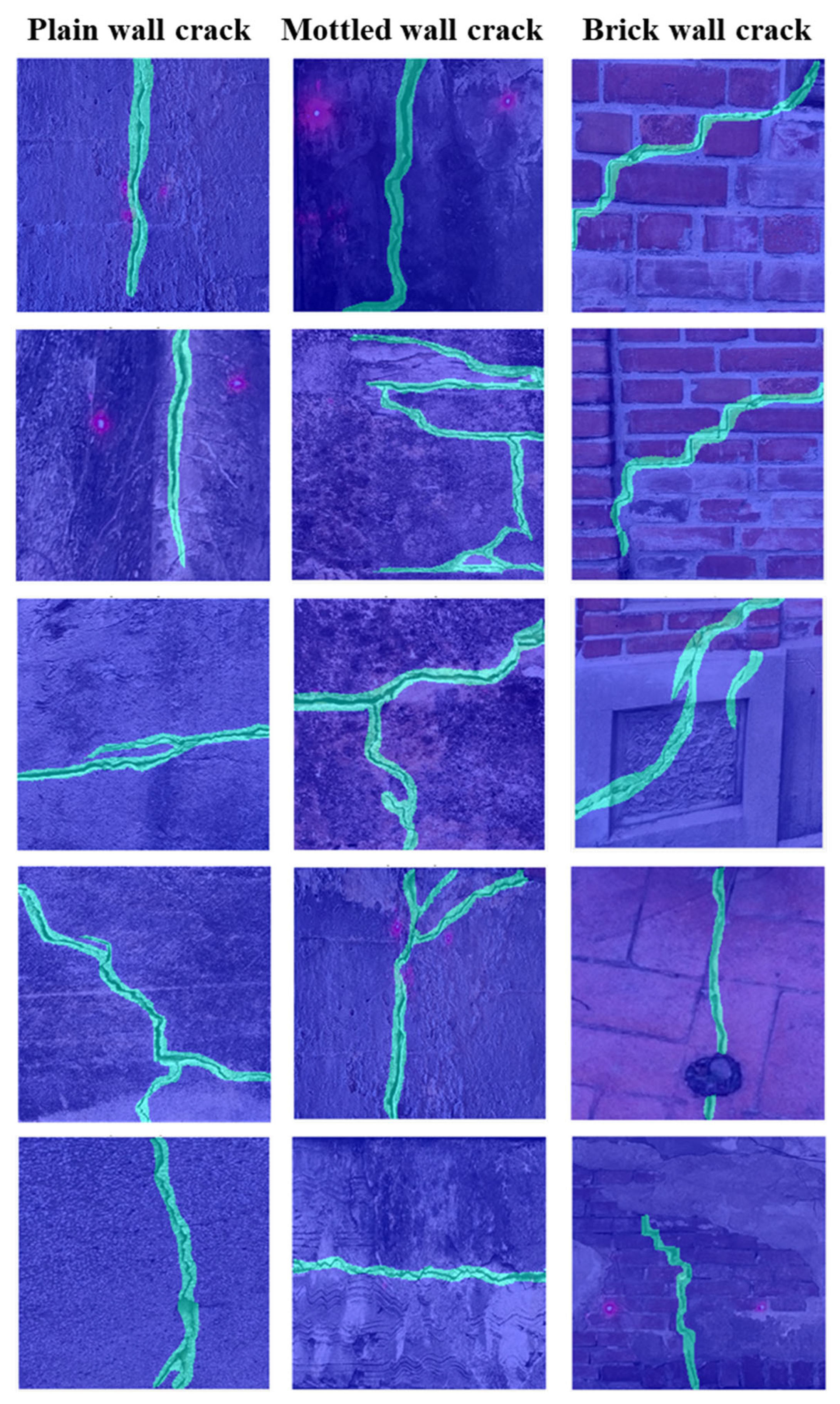
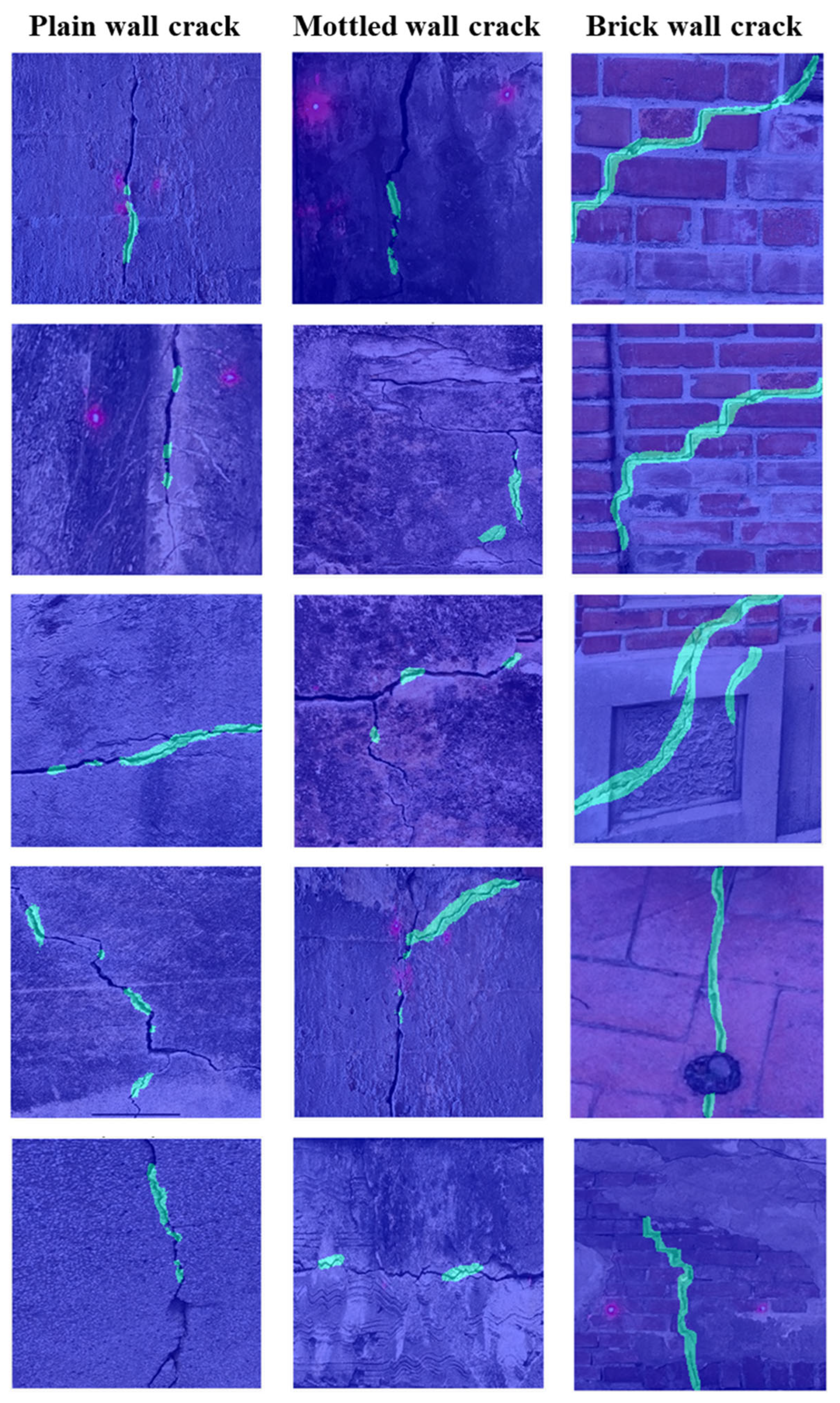
3.2. Pixel-Level Segmentation of Crack Regions

The SegNet deep learning model was utilized for crack segmentation in cultural heritage images to assess structural integrity. The model was trained on a dataset of 300 images, employing a 70:30 split for training and validation. Before conducting the overall training and validation of SegNet, K-fold cross-validation was also performed. The IoU values from the five validations were 0.798, 0.823, 0.857, 0.815, and 0.866, respectively. The difference between the maximum and minimum values was less than 0.1, indicating that the distribution of different image patterns in the training set was relatively balanced, without excessive concentration.

Performance metrics, including training accuracy, validation accuracy, training loss, and validation loss, were recorded across 75,000 iterations. Initially, the training accuracy was measured at 61.48% and increased to 98.11% within 1000 iterations. It stabilized above 98.5% by 2000 iterations and reached 99.29% at 45,000 iterations, demonstrating robust learning capability and stability (Figure 4a). Similarly, validation accuracy improved from 62.35% to 98.06% after 1000 iterations and stabilized at 98.62% beyond 45,000 iterations, indicating strong generalization performance.

Training loss, initially recorded at 0.763, reflecting a high prediction error, steadily declined to 0.019 at 45,000 iterations (Figure 4b). Validation loss followed a similar trend, decreasing from 0.762 to 0.052, demonstrating consistent error minimization. However, at 75,000 iterations, training accuracy reached 99.99%, while validation accuracy declined slightly to 99.39%. Training loss dropped to 0.001, whereas validation loss increased to 0.083, suggesting potential overfitting.

The model trained at 45,000 iterations was selected for further analysis, as it demonstrated the optimal trade-off between accuracy and generalization, achieving an Intersection over Union (IoU) of 0.832. To further assess the model’s generalization performance, an external dataset [53] comprising 237 images was employed for validation. The resulting IoU of 0.726 suggests that, although the SegNet model exhibited reduced performance on external data compared to internal validation, it nonetheless maintained a reasonable level of predictive capability.

Figure 5 presents the results of semantic segmentation, demonstrating the model’s capability to effectively differentiate crack regions (green) from non-crack regions (red). In Figure 5a, certain fine cracks remain undetected, as indicated by the blue box. This limitation is primarily attributed to the loss of detail during image downscaling, which causes narrow cracks to fall below the model’s detection threshold. This issue may be mitigated by increasing image resolution, capturing images at a closer distance, or performing segmentation directly on the original high-resolution images. Alternatively, image preprocessing techniques, such as contrast enhancement or the application of sharpening filters, can improve crack visibility and facilitate more accurate segmentation.

3.3. Crack Length Estimation Analysis

The GoogleNet model was employed for crack detection, followed by SegNet for segmentation. Crack length estimation was performed using two parallel laser points spaced 15 cm apart as reference markers. Two case studies were conducted to validate this methodology (Figure 6), comparing SegNet-based estimations with actual measurements.

In Figure 6b, the endpoints of Crack A (black dots) exhibited a pixel difference of 169, while the laser points (yellow dots) showed a difference of 66 pixels, corresponding to a real-world distance of 15 cm. This resulted in a pixel-to-distance ratio of 1 pixel = 0.22 cm, yielding an estimated crack length of 37.18 cm. The actual measured length was 38.4 cm, with a discrepancy of 1.22 cm and an accuracy of 97%. Similarly, in Figure 6c,d, the endpoints of Crack B displayed a pixel difference of 223, while the laser points exhibited a 134-pixel difference, equating to 1 pixel = 0.11 cm. The estimated crack length was 24.53 cm, whereas the actual measured length was 25.3 cm, with a discrepancy of 0.77 cm and an accuracy of 97%.

Four primary sources of error contribute to the results presented above: (1) segmentation error from the deep learning-based SegNet model, (2) pixel discretization error arising from manual selection of laser points in the image, (3) laser misalignment error due to imperfect parallelism between the dual-laser beams, and (4) image capture error resulting from non-perpendicular viewpoints during image acquisition.

Regarding image capture error, when a horizontal crack is imaged using a forward-tilted smartphone, no distortion occurs if the crack lies at the vertical center of the image. However, if the crack appears in the upper half, it undergoes compression due to perspective distortion. For example, when a crack is located at v = 1 and the camera is tilted by 5°, the measured crack length is underestimated by approximately 0.38%. Conversely, cracks in the lower half of the image (e.g., v = 256) are stretched, leading to an overestimation of similar magnitude under the same tilt. In the case of vertical cracks distributed symmetrically in the upper and lower halves, the distortion effects tend to cancel out, resulting in negligible overall error.

Laser misalignment error occurs when the two laser beams are not perfectly parallel or not aligned on the same plane as the surface of the crack. Such misalignment affects the apparent spacing between laser dots in the image, thereby distorting the reference scale. For instance, a ±5° inward tilt of the lasers results in a projected spacing ranging from approximately 14.94 cm to 15.06 cm (a ±0.4% deviation), leading to a corresponding underestimation of crack length.

A pixel discretization error arises from uncertainty in localizing the laser points, particularly when the dots appear slightly blurred or diffused. In the conducted experiments, the pixel distances between laser dots were 66 pixels for Crack A and 134 pixels for Crack B. Assuming an uncertainty of ±1 pixel, the resulting relative error is approximately ±1.52% for Crack A and ±0.75% for Crack B.

These discretization and misalignment errors may either accumulate or partially offset one another. Considering that the overall measurement accuracy in Examples A and B reached approximately 97%, the segmentation error introduced by the SegNet model is estimated to contribute between 0.7% and 3.0% of the total error. These findings support the reliability and applicability of using SegNet in conjunction with laser markers for crack detection and length estimation.

Furthermore, the impact of pixel discretization, laser misalignment, and image capture errors can be mitigated through several strategies: increasing image resolution, maintaining equal front and rear distances between the dual lasers to preserve parallel alignment, and applying geometric rectification to correct for perspective distortion.

3.4. Crack Detection Limit Analysis

To assess the performance limitations of SegNet in crack analysis, this study employed a single original image, which was progressively downscaled to various resolutions for semantic segmentation. As illustrated in Figure 7, the first row displays the original image reduced to 224 × 224 pixels. The second row presents the image downscaled to 425 × 425 pixels, subsequently divided into 224 × 224 pixel tiles. The third row follows the same procedure with an image size of 850 × 850 pixels. The fourth and fifth rows show the image downscaled to 1700 × 1700 pixels and segmented into 224 × 224 pixel patches.

In Figure 7, blue boxes delineate the coverage areas corresponding to the subsequent row’s images, while yellow boxes highlight regions where cracks were no longer detected following downsampling. The results indicate that when the resolution is reduced from 1700 × 1700 to 850 × 850 pixels, SegNet fails to detect four crack regions. Further reduction to 425 × 425 pixels results in the loss of one additional crack region. When the resolution is further downscaled to 224 × 224 pixels, two more crack regions remain undetected. Upon examination of the yellow-marked areas and their corresponding downsampled versions, it was observed that cracks narrower than two pixels tend to become undetectable by SegNet.

4. Discussion

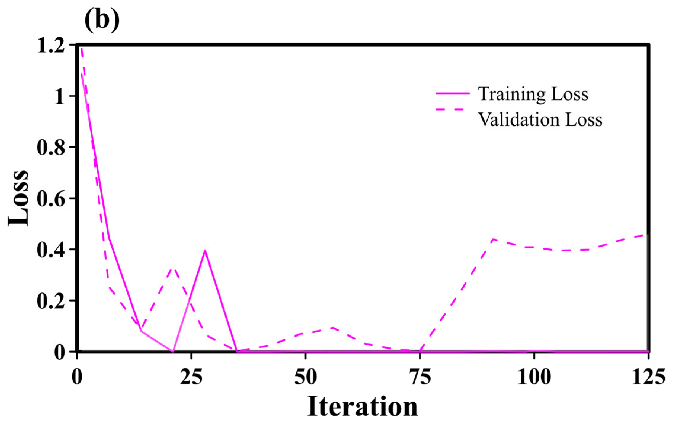
4.1. Number of Iterations

The number of iterations is a critical parameter in deep learning model training, directly influencing the model’s learning effectiveness, generalization ability, and overall performance. This section examines the impact of iteration count on both the crack detection model (GoogleNet) and the semantic segmentation model (SegNet).

4.1.1. Impact of Iteration Count on GoogleNet

This subsection investigates the performance of the GoogleNet model across different iteration counts. A dataset of 66 images was used, consisting of 11 images of general wall cracks, 11 images of weathered wall cracks, 11 images of brick wall cracks, and 33 images without cracks. The model was trained and validated over 25, 50, 75, 100, and 125 iterations, with 70% of the images used for training and 30% for validation. To further evaluate the model’s performance, an additional set of 34 images (including six images each of general wall cracks, weathered wall cracks, and brick wall cracks, along with 16 images without cracks) was used for application analysis. The results were assessed using comprehensive evaluation metrics.

Figure 8 presents the training and validation results of the GoogleNet model across different iteration counts, including accuracy and loss metrics. Figure 9 illustrates the comprehensive evaluation metrics, including accuracy, precision, and F1-score.

At 25 iterations, the training and validation accuracies were 90% and 70%, respectively, with training and validation losses of 0.573 and 0.963. The comprehensive evaluation metrics yielded an accuracy of 70%, precision of 62.50%, recall of 100%, and an F1-score of 0.769. While the model performed well on the training data, its performance on validation data was relatively poor, indicating that it learned the training data effectively but struggled with unseen data. Although the model successfully detected cracks, it exhibited a high false positive rate.

At 50 iterations, the training and validation accuracies improved to 90% and 97.83%, respectively, with training and validation losses decreasing to 0.088 and 0.024. The evaluation metrics showed an accuracy of 97.83%, precision of 95.65%, recall of 100%, and an F1-score of 0.978. As the iteration count increased, the model’s validation accuracy improved significantly, approaching 100%. The reduction in training and validation loss further demonstrated enhanced generalization ability, allowing the model to better handle unseen data while significantly reducing false positives. At 75 iterations, the model achieved 100% accuracy on both the training and validation datasets, with near-zero loss, indicating exceptionally high precision and stability. All evaluation metrics, including accuracy, precision, recall, and F1-score, reached 100%, suggesting that the model had attained its optimal state. At this iteration count, the model perfectly detected cracks without false positives, achieving the best overall performance.

At 100 iterations, the training accuracy remained at 100%, while validation accuracy decreased to 93.48%, with training and validation losses recorded at 0.0003 and 0.199, respectively. The evaluation metrics showed an accuracy of 95.65%, precision of 92.31%, recall of 100%, and an F1-score of 0.96. Although the model maintained perfect performance on the training data, its validation performance declined, suggesting the onset of overfitting. At 125 iterations, the training accuracy remained at 100%, but the validation accuracy further declined to 90%. Training and validation losses were recorded at 0.0002 and 0.46, respectively. The evaluation metrics showed an accuracy of 90%, precision of 83.33%, recall of 100%, and an F1-score of 0.909. The increasing validation loss and declining validation accuracy indicated a more pronounced overfitting effect, where the model over-adapted to the training data at the expense of generalization. Consequently, the model’s precision in crack detection decreased, leading to a higher false positive rate.

Based on the evaluation across different iteration counts, the model demonstrated its optimal performance at 75 iterations, achieving perfect training and validation accuracy, minimal training and validation loss, and ideal evaluation metrics. However, as the iteration count increased to 100 and 125, overfitting became evident, with validation accuracy declining to 93.48% and 90%, respectively, and validation loss increasing significantly. This decline in generalization ability highlights the risk of excessive iteration, which can compromise the model’s effectiveness on a new dataset.

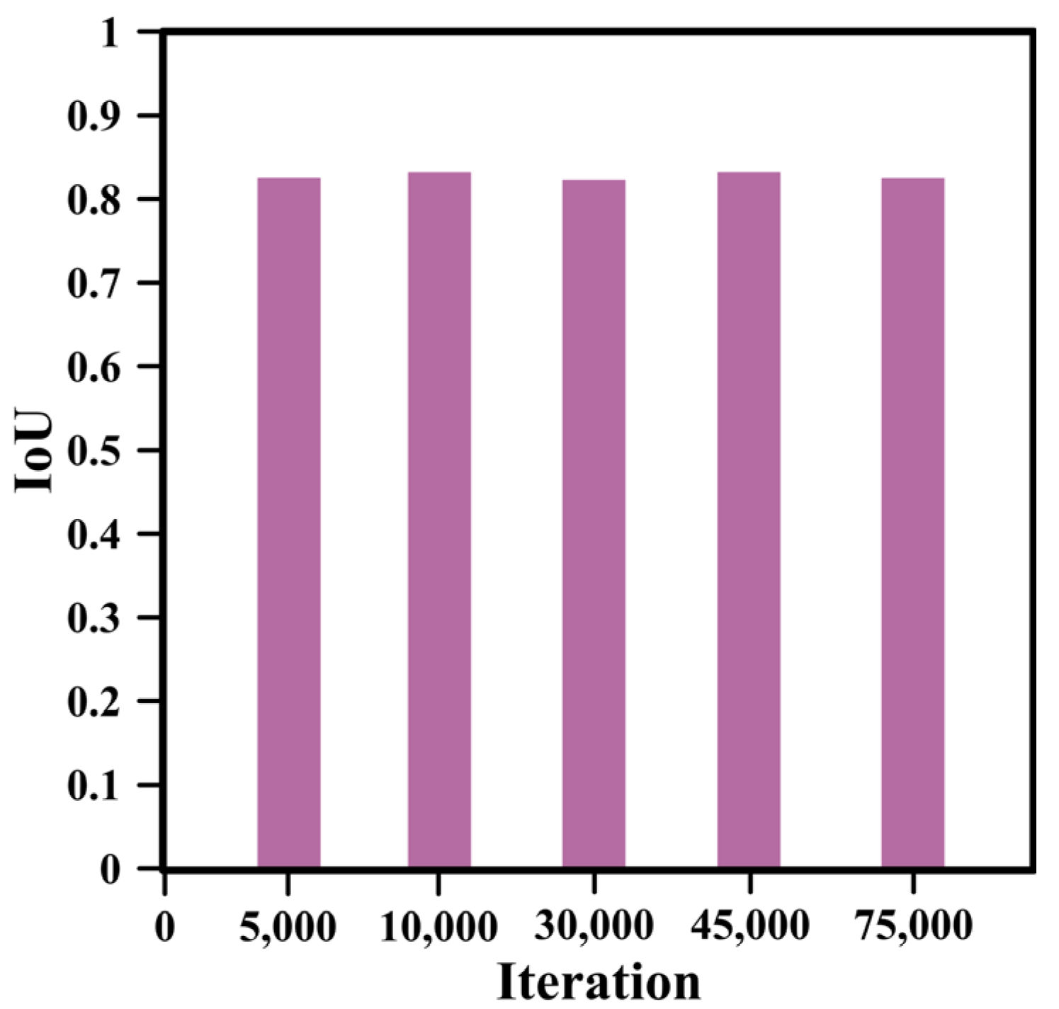
4.1.2. Impact of Iteration Count on SegNet

This subsection examines the performance of the SegNet model in semantic segmentation of crack images across different iteration counts. The model was trained using five iteration settings: 5000, 10,000, 30,000, 45,000, and 75,000 iterations. A dataset of 300 images was used, generated by augmenting 50 original images comprising 17 images of general wall cracks, 17 images of weathered wall cracks, and 16 images of brick wall cracks. The dataset was split into 70% for training and 30% for validation. Performance metrics, including training and validation accuracy as well as training and validation loss, were recorded. Additionally, 15 original images comprising five images each of general wall cracks, weathered wall cracks, and brick wall cracks were used for application analysis, with model performance evaluated using the Intersection over Union (IoU) metric.

Figure 10 presents the training and validation results of the SegNet model across different iteration counts, including accuracy and loss. Figure 11 displays the IoU results for each iteration count. At 5000 iterations, the training and validation accuracies were 99.01% and 98.47%, respectively, with training and validation losses of 0.331 and 0.338. These results indicate strong model performance; however, the relatively high loss values suggest room for further optimization. The IoU score of 0.825 reflects good segmentation accuracy, demonstrating the model’s ability to effectively detect and segment cracks while still allowing for potential improvement.

At 10,000 iterations, training and validation accuracies slightly adjusted to 98.72% and 98.53%, with corresponding losses of 0.214 and 0.225. The significant reduction in training and validation loss indicates enhanced convergence performance, while accuracy remains at a high level. The IoU score increased slightly to 0.832, suggesting an improvement in segmentation precision. At 30,000 iterations, training and validation accuracies further improved to 98.88% and 98.62%, with losses decreasing to 0.045 and 0.066. These results demonstrate stronger convergence and generalization. However, the IoU score declined slightly to 0.823, suggesting that despite improvements in accuracy, the model’s segmentation performance in practical application showed a slight reduction.

At 45,000 iterations, training and validation accuracies reached 99.13% and 98.62%, while losses decreased significantly to 0.019 and 0.052. These results indicate that the model achieved high precision and stability. The IoU score remained at 0.832, marking the best observed segmentation performance. At 75,000 iterations, the training accuracy approached 99.99%, while validation accuracy increased to 99.39%. However, validation loss increased slightly to 0.083, indicating the emergence of mild overfitting. The IoU score measured 0.826, suggesting that excessive iteration may have slightly degraded the model’s generalization performance.

Overall, across all iteration settings, training and validation accuracies consistently exceeded 98%, while training loss continued to decrease as iterations increased. However, validation loss was minimized at 45,000 iterations, and the best IoU evaluation results were also achieved at this point. These findings indicate that at 75,000 iterations, the model exhibited signs of overfitting. Therefore, the optimal iteration count for SegNet in this study is determined to be 45,000.

This study found that GoogleNet and SegNet produced identical results. A higher number of iterations does not necessarily lead to better performance; excessive iterations may result in overfitting. These findings are consistent with the results of [54,55].

4.2. Number of Images

This section explores the impact of different image quantities on the learning efficiency and performance of the crack detection model (GoogleNet) and the semantic segmentation model (SegNet).

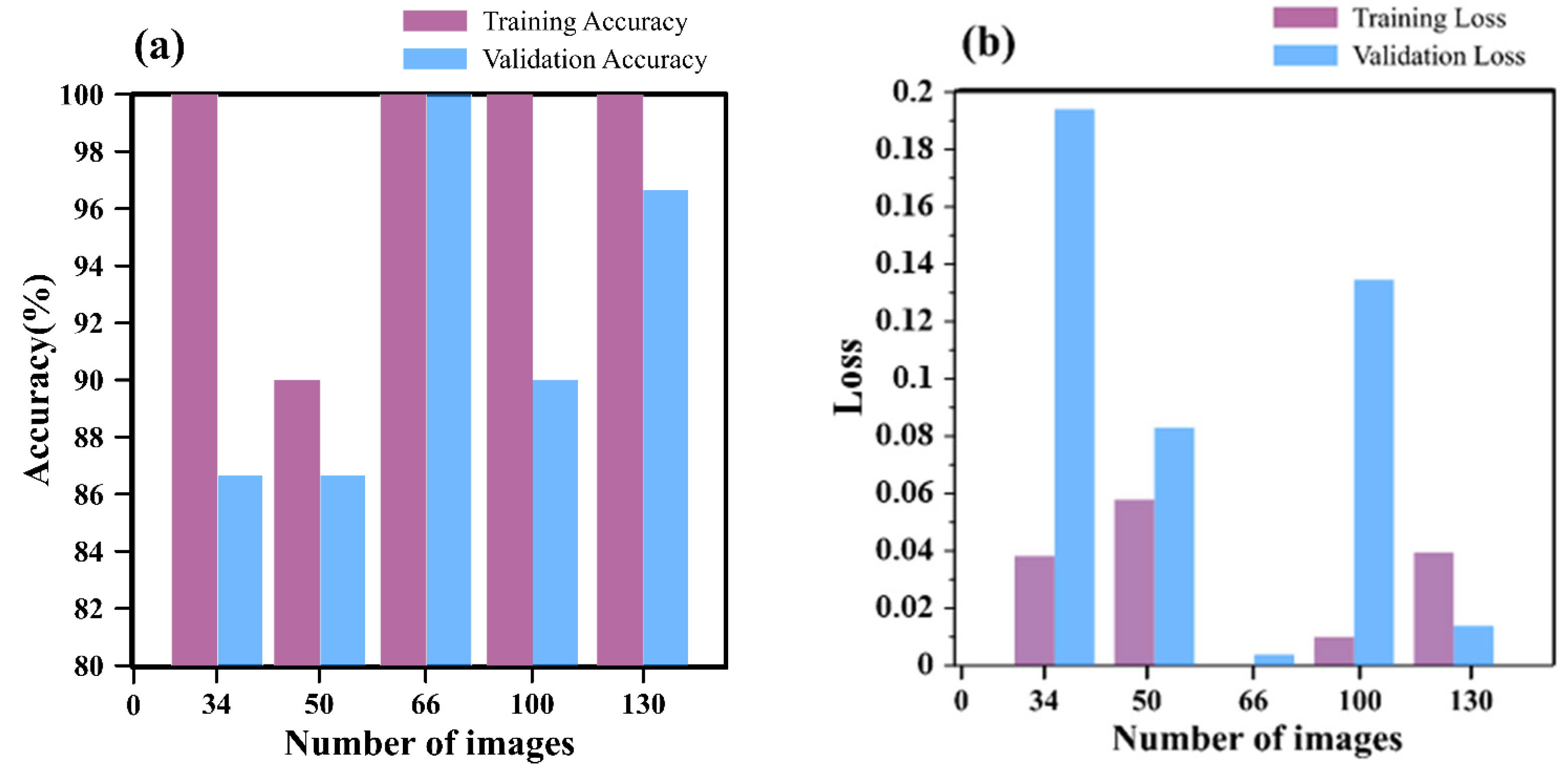
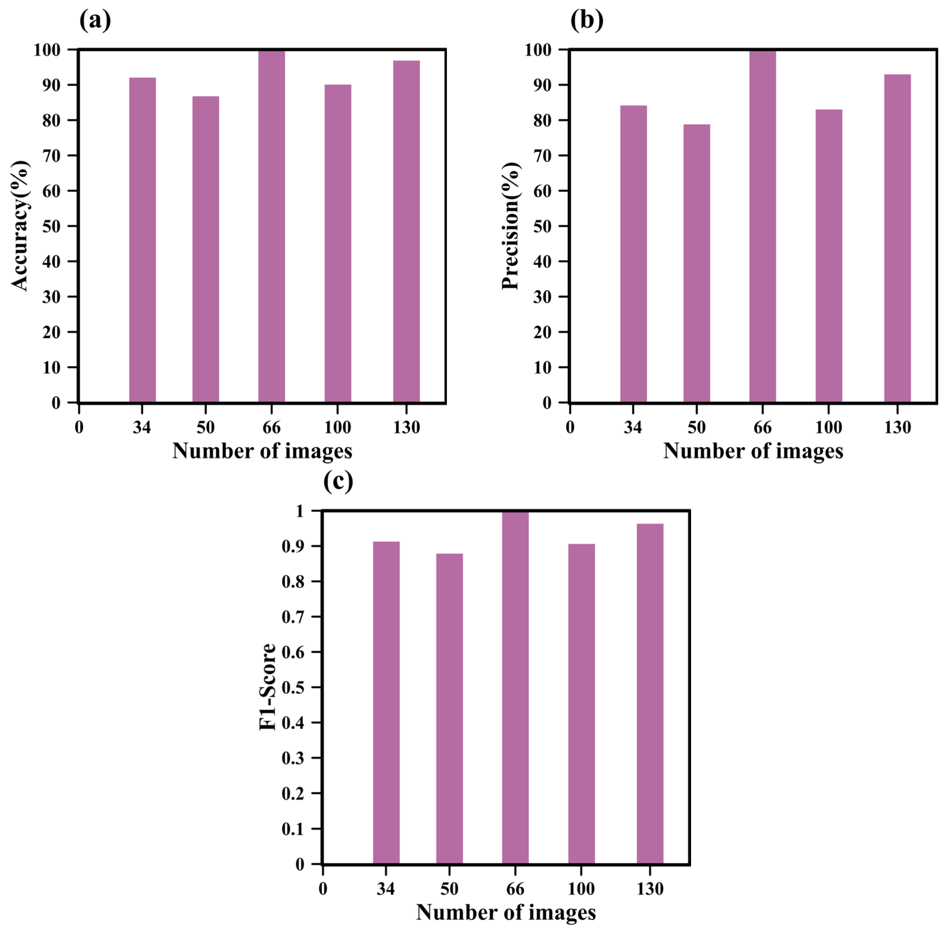
4.2.1. Impact of Image Quantity on GoogleNet

To assess the performance of the GoogleNet model under varying image quantities, datasets of 34, 50, 66, 100, and 130 images were used, with 70% allocated for training and 30% for validation. The number of images in each category is detailed in

Table 3. Using GoogleNet on different images and different types of images.

Number of Images for Training and Validation	Images of Plain Wall Crack	Images of Mottled Wall Crack	Images of Brick Wall Crack	Images with Crack
34	6	6	5	17
50	9	8	8	25
66	11	11	11	33
100	17	17	16	50
130	22	22	21	65

. The model was trained and validated using the optimal iteration count (75) to evaluate the effect of image quantity on learning capability.

The trained GoogleNet model was further tested on an independent set of 34 images, comprising six images of cracks on plain walls, six on mottled walls, six on brick walls, and 16 without cracks. Model performance was assessed using comprehensive evaluation metrics. Figure 12 presents the training and validation results for different image quantities, while Figure 13 illustrates the corresponding evaluation metrics.

With 34 images used for training and validation, the training and validation accuracies were 100% and 86.67%, respectively, with training and validation losses of 0.0383 and 0.194. Although the training accuracy reached 100%, the relatively lower validation accuracy and higher validation loss indicate poor generalization ability. The comprehensive evaluation metrics yielded an accuracy of 91.67%, precision of 84.62%, recall of 100%, and an F1-score of 0.917. While the model successfully detected all cracks, it exhibited a high false positive rate, highlighting the need for improved precision and stability. When trained and validated with 50 images, the training and validation accuracies were 90% and 86.67%, respectively, with losses of 0.058 and 0.083. While the training accuracy decreased slightly, the validation accuracy remained unchanged, and the validation loss showed minor improvement. However, the model’s generalization ability was still insufficient. The evaluation metrics indicated an accuracy of 86.67%, precision of 78.95%, recall of 100%, and an F1-score of 0.882. The drop in precision and F1-score suggests that further optimization is needed, even with an increased number of training images.

For the model trained and validated with 66 images, the training and validation accuracies were 100% and 100%, respectively, with losses of 0.0001 and 0.004. Notably, all evaluation metrics—accuracy, precision, recall, and F1-score—reached their highest values, indicating superior model performance under this condition. Using 100 images for training and validation, the model achieved training and validation accuracies of 100% and 90%, with losses of 0.01 and 0.135. Both training and validation accuracies improved, and validation loss significantly decreased, demonstrating enhanced generalization ability. The evaluation metrics showed an accuracy of 90%, precision of 83.33%, recall of 100%, and an F1-score of 0.909. Although precision and F1-score slightly declined, overall performance remained at a high level. When trained and validated with 130 images, the training and validation accuracies were 100% and 96.67%, respectively, with losses of 0.04 and 0.014. The evaluation metrics showed an accuracy of 96.67%, precision of 93.33%, recall of 100%, and an F1-score of 0.968.

Among all tested configurations, the model trained and validated with 66 images demonstrated the best evaluation performance when analyzing the independent set of 34 images, achieving 100% accuracy, precision, recall, and F1-score. This suggests that training with 66 images yields the most stable and accurate results, ensuring excellent learning and generalization capabilities.

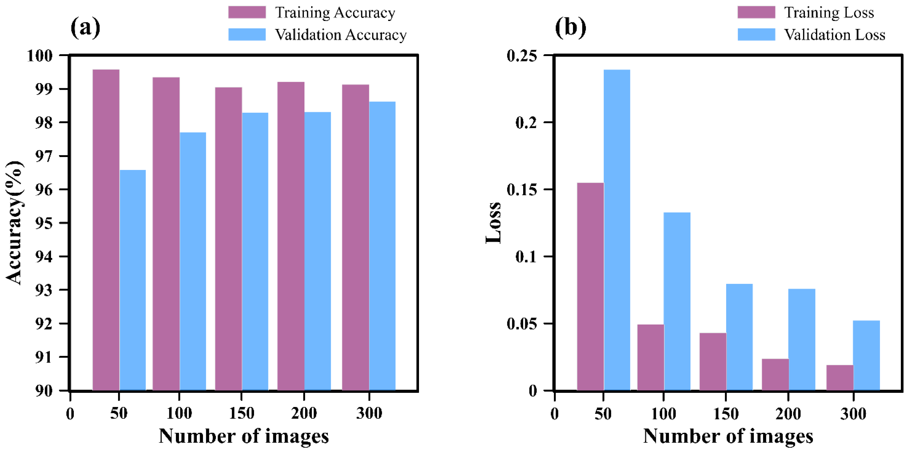
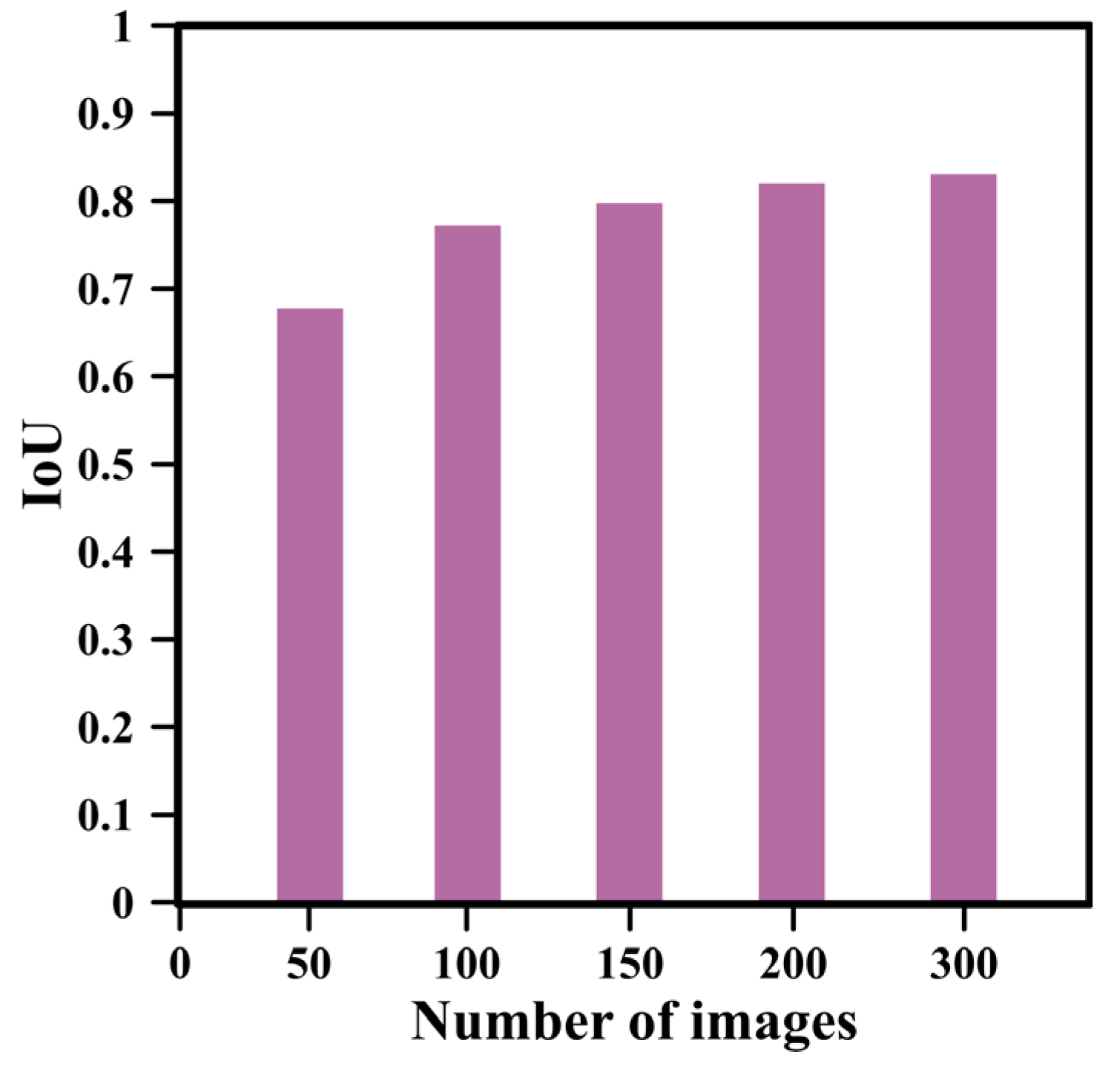
4.2.2. Impact of Image Quantity on SegNet

This section examines the impact of varying image quantities on the performance of the SegNet model for wall crack detection. The original dataset comprised 50 images, including 17 images of cracks on plain walls, 17 on mottled walls, and 16 on brick walls. To enhance model stability and adaptability, data augmentation techniques (such as rotation, flipping, cropping, and scaling) were applied to generate additional training samples and expand the training dataset. Additionally, an independent set of 15 images (five images each of cracks on plain walls, mottled walls, and brick walls) was used for application analysis. The model’s performance was evaluated using the Intersection over Union (IoU) metric.

Based on the findings in Section 4.1.2, the optimal iteration count of 45,000 was used for training. The accuracy, loss, and IoU values were recorded across five different image quantities: 50, 100, 150, 200, and 300 images. The dataset was split into 70% for training and 30% for validation. Figure 14 and Figure 15 illustrate the training/validation results and analysis of SegNet performance under different image quantities.

When trained and validated with 50 images, the model achieved training and validation accuracies of 99.58% and 96.59%, respectively, with training and validation losses of 0.155 and 0.2393. While the accuracy demonstrated strong performance, the relatively high loss values indicated room for improvement. The IoU value was 0.678, suggesting suboptimal segmentation performance. With 100 training images, the model’s training and validation accuracies were 99.35% and 97.71%, with losses reduced to 0.049 and 0.133. The IoU value increased to 0.772, indicating a notable improvement in segmentation capability.

For 150 training images, the model achieved training and validation accuracies of 99.05% and 98.30%, with losses of 0.043 and 0.08. The further reduction in loss values indicated improved stability, and the IoU value increased to 0.798, reflecting enhanced segmentation performance. With 200 training images, the training and validation accuracies were 99.21% and 98.32%, while the loss values further declined to 0.024 and 0.76. Also, the IoU value increased to 0.82. This continued reduction in loss suggests improved generalization ability. When trained with 300 images, the model achieved its highest accuracy, with training and validation accuracies of 99.13% and 98.62%, respectively. The loss values were at their lowest (0.019 and 0.052), and the IoU value reached its peak at 0.832, demonstrating the best overall segmentation performance.

A comparison of SegNet’s performance across different image quantities indicates that increasing the number of images leads to consistent improvements in model performance for both training and validation datasets. Training with 300 images yielded the highest accuracy, the lowest loss, and the best IoU score. This finding aligns with Luca et al. [56], who reported that increasing dataset size enhances model generalization and accuracy by providing richer feature learning. However, larger datasets also introduce higher computational costs and longer training times. Additionally, the diversity of image types plays a crucial role in model performance. Training on a diverse dataset improves the model’s adaptability and accuracy across different image types, reducing misclassification rates.

4.3. Image Categories

The performance of crack detection and semantic segmentation models varies significantly depending on the type of images being processed. This section explores the impact of different image categories on model performance.

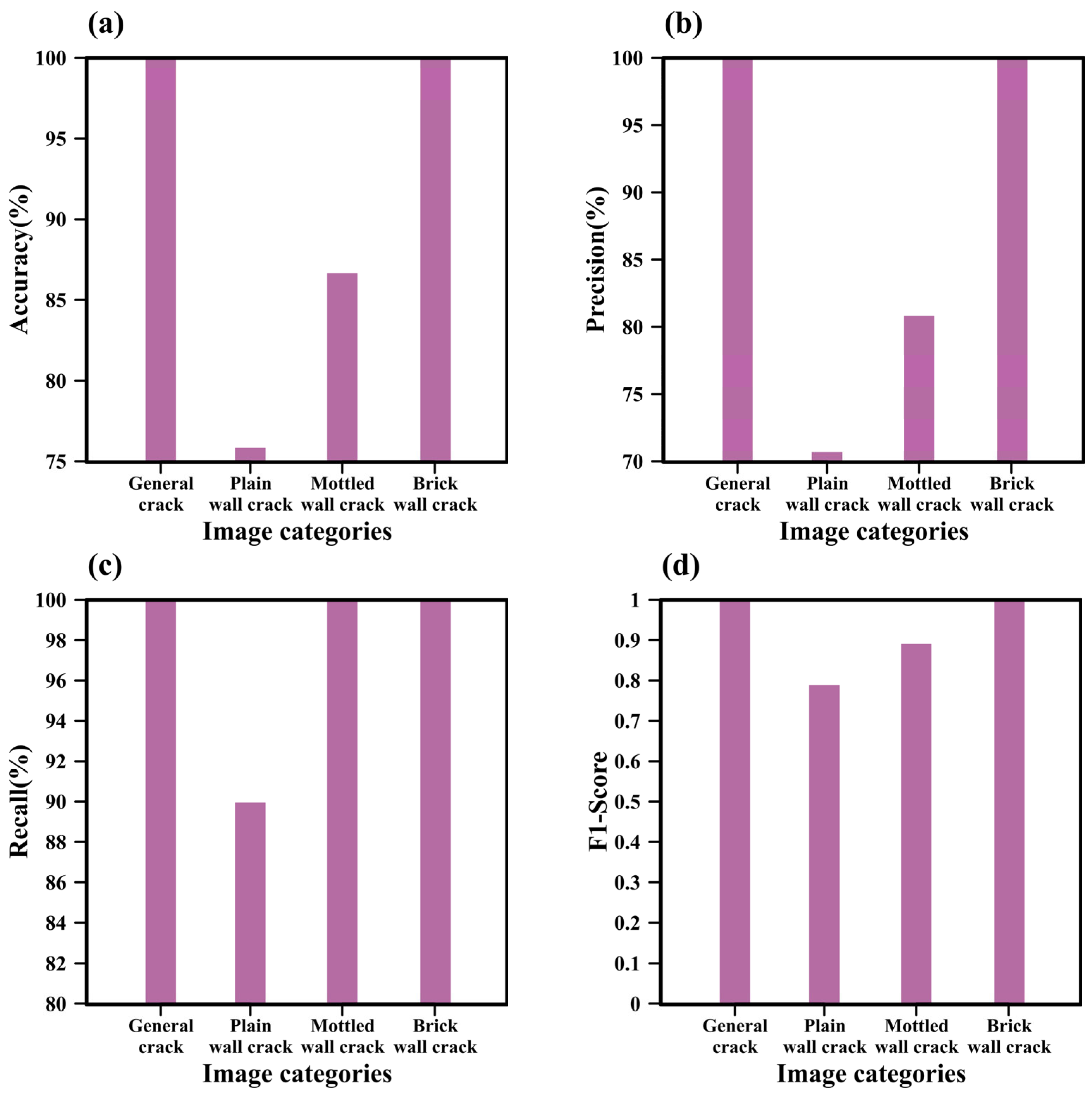
4.3.1. Impact of Image Categories on GoogleNet

This study evaluates three different types of crack images: cracks on plain walls, cracks on mottled walls, and cracks on brick walls. Four separate GoogleNet models were trained using different datasets. (1) General crack detection model trained on 66 images, including 11 images for each crack type and 33 non-crack images. (2) Plain wall crack model trained on 66 images, consisting of 33 crack images (expanded from 16 original images using data augmentation) and 33 non-crack images. (3) Mottled wall crack model trained on 66 images, consisting of 33 crack images (expanded from 16 original images) and 33 non-crack images. (4) Brick wall crack model trained on 66 images, consisting of 33 crack images (expanded from 15 original images) and 33 non-crack images.

Each dataset was split into 70% for training and 30% for validation, with 75 training iterations. After training and validation, an additional 34 images (six plain wall crack images, six mottled wall crack images, six brick wall crack images, and 16 non-crack images) were used for application analysis, and the results were assessed using comprehensive evaluation metrics. Figure 16 and Figure 17 present the training, validation, and comprehensive evaluation results for GoogleNet across different image categories. For the general crack detection model, both training and validation accuracies reached 100%, with training and validation losses of 7.2242 × 10⁻⁶ and 0.0038, respectively. The comprehensive evaluation metrics showed an accuracy of 100%, precision of 100%, recall of 100%, and an F1-score of 1.0, indicating perfect performance.

For the plain wall crack model, training and validation accuracies were 100% and 84.85%, with training and validation losses of 0.002 and 0.626. The evaluation metrics showed an accuracy of 75.85%, precision of 70.75%, recall of 90%, and an F1-score of 0.79. While the model achieved perfect accuracy in training, its validation accuracy was lower, and the high validation loss suggested overfitting. The relatively low F1-score indicated room for improvement in handling this image type.

For the mottled wall crack model, training and validation accuracies were 100% and 91.3%, with training and validation losses of 6.2705 × 10⁻⁶ and 0.257. The evaluation metrics showed an accuracy of 86.65%, precision of 80.95%, recall of 100%, and an F1-score of 0.895. This model demonstrated high accuracy and lower validation loss, suggesting better generalization. The F1-score, approaching 0.9, indicated strong performance in this category.

For the brick wall crack model, both training and validation accuracies were 100%, with training and validation losses of 8.2255 × 10⁻⁶ and 0.0063. The evaluation metrics showed 100% accuracy, precision, recall, and an F1-score of 1.0. This model performed exceptionally well, achieving perfect results with minimal loss, indicating outstanding capability in detecting cracks on brick walls.

An analysis of different image categories revealed a significant impact on GoogleNet’s performance. The best results were obtained when the dataset included all image categories. The brick wall crack model performed second-best, achieving the same perfect evaluation results as the general crack detection model in application analysis. In contrast, the plain wall and mottled wall crack models exhibited weaker generalization, as indicated by lower validation accuracy and higher validation loss, despite achieving high training accuracy. Their evaluation metrics, including accuracy, precision, recall, and F1-score, did not reach optimal levels.

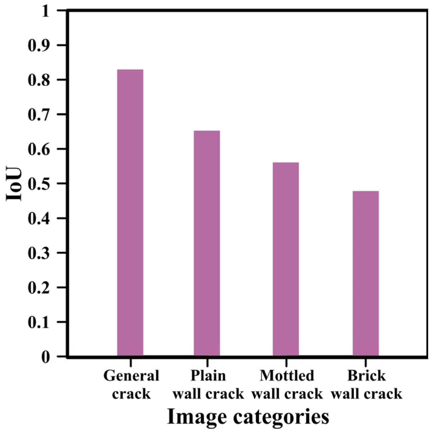
4.3.2. Impact of Image Categories on SegNet

This section investigates the influence of different crack image categories on the performance of the SegNet model. Four distinct datasets were used for model training. (1) General crack image model: This dataset includes all crack image types, consisting of 17 plain wall crack images, 17 mottled wall crack images, and 16 brick wall crack images, expanded to 300 images through data augmentation. (2) Plain wall crack model: This dataset includes only plain wall crack images, originally 17 images, expanded to 300 through data augmentation. (3) Mottled wall crack model: This dataset includes only mottled wall crack images, originally 17 images, expanded to 300 through data augmentation. (4) Brick wall crack model: This dataset includes only brick wall crack images, originally 16 images, expanded to 300 through data augmentation.

Each model was trained and validated over 45,000 iterations. Following training and validation, an additional 15 images (five plain wall crack images, five mottled wall crack images, and five brick wall crack images) were used for IoU analysis (see Figure 18, Figure 19, Figure 20 and Figure 21).

Figure 22 presents the training and validation results for SegNet models trained on different image categories, while Figure 23 shows the IoU results for application analysis. Among the four SegNet models, the general crack image model achieved the best performance, with training and validation accuracies of 99.13% and 98.62%, respectively. Training and validation losses were 0.019 and 0.052, with an IoU of 0.832. These results indicate high accuracy and stability in processing various crack image types.

The plain wall crack model achieved training and validation accuracies of 98.93% and 98.07%, respectively, with training and validation losses of 0.079 and 0.096, and an IoU of 0.656. While the model demonstrated high accuracy and stability, the relatively high loss values suggest room for improvement in precision for this image type.

The mottled wall crack model showed training and validation accuracies of 98.98% and 98.21%, respectively, with training and validation losses of 0.021 and 0.063, and an IoU of 0.563. Despite high accuracy and relatively low loss values, its IoU performance was suboptimal.

The brick wall crack model achieved training and validation accuracies of 99.1% and 98.26%, respectively, with training and validation losses of 0.024 and 0.064, and an IoU of 0.48. Although the model exhibited high accuracy, the lowest IoU value among all models indicates weaker segmentation performance for this category.

Overall, the general crack image model provided the best results, achieving the highest training and validation accuracies with the lowest losses and the best IoU score in application analysis. The three category-specific models, while maintaining over 98% accuracy and loss values below 0.1, exhibited weaker generalization, as reflected in their IoU scores of 0.656, 0.563, and 0.48 for the plain wall, mottled wall, and brick wall models, respectively.

Figure 18, Figure 19, Figure 20 and Figure 21 illustrate the analysis of 15 crack images using different models. The general crack image model effectively identified crack locations and regions across various image types (Figure 18). In contrast, models trained on a single image category performed well only on images with similar characteristics to their training data. For instance, the plain wall crack model performed well on five plain wall crack images (Figure 19), accurately identifying crack regions in four images, with only one misclassification. However, it struggled with mottled wall crack images, correctly identifying cracks in only two out of five images, and performed poorly on brick wall crack images due to their complex textures.

Similarly, the mottled wall crack model achieved near-perfect segmentation for mottled wall cracks (Figure 20), correctly identifying cracks in four out of five images. It also performed reasonably well on plain wall cracks, recognizing approximately 80% of crack regions. However, its performance on brick wall images was poor. The brick wall crack model, as shown in Figure 21, excelled at identifying cracks in brick wall images but could only detect limited crack regions in plain and mottled wall images.

In contrast to GoogleNet, which performed best with both the general crack image model and the brick wall crack model, SegNet achieved optimal results only when trained on the general crack image model. This discrepancy may be attributed to the structural complexity of brick walls, where mortar joints could mislead the analysis when using models trained only on plain or mottled wall cracks. These findings align with the results reported by [56].

4.3.3. Texture Analysis

To further investigate the significant variation in model performance across different wall types, a texture and feature analysis was conducted using Gray-Level Co-occurrence Matrix (GLCM) metrics.

Crack images on plain walls typically exhibit smooth and uniform background textures, resulting in high contrast between cracks and the surrounding surface. This facilitates precise crack identification. GLCM analysis supports this observation, with a low contrast value of 0.41 and high homogeneity of 0.85 (Figure 24), indicating minimal texture variation and a consistent grayscale distribution—conditions favorable for accurate segmentation.

In contrast, crack images on mottled walls present irregular textures, stains, and spot patterns that may resemble cracks, increasing the risk of misclassification. Corresponding GLCM values indicate a high contrast of 2.79, low energy of 0.03, and moderate homogeneity of 0.58 (Figure 24), reflecting high background complexity and considerable grayscale variation, both of which challenge the segmentation capabilities of models such as SegNet.

For brick walls, while the background texture is relatively consistent, geometric interference from brick patterns and mortar joints complicates the analysis. GLCM results show a moderate contrast of 0.86, the highest correlation (0.88), and a lower homogeneity of 0.66 compared to plain walls (Figure 24). These metrics indicate a structurally repetitive grayscale pattern. However, such repetition can lead to confusion between cracks and structural edges, causing the model to misclassify mortar lines as cracks or to fragment continuous cracks.

These findings highlight that segmentation models trained on crack images from a single wall type may struggle to generalize across other surface types, due to inherent differences in texture characteristics.

4.4. Comparison with Other Deep Learning Models

In deep learning, model performance is often related to the number of parameters, which represent trainable weights and biases. The GoogleNet classification model contains approximately 6.8 million parameters, while the SegNet segmentation model has about 14.7 million parameters; the MATLAB implementation of SegNet includes approximately 6 million. These represent significant reductions compared to earlier models such as AlexNet (∼60 million parameters) for classification and VGG16 (∼134 million) for segmentation. However, compared to more recent lightweight architectures designed for mobile deployment, such as MobileNetV3-BLS (∼6 million parameters) for classification and ENet (∼0.4 million) for segmentation, GoogleNet and SegNet are relatively larger.

The MobileNetV3-BLS model has achieved strong performance in classification tasks, with reported accuracy of 98.9%, precision of 100%, recall of 93.8%, and an F1-score of 0.968 when trained on a dataset of over 6000 images [57]. ENet, applied to wall surface segmentation tasks including cracks, efflorescence, rebar exposure, and spalling, has achieved an IoU of 0.45 for crack segmentation [58]. While MobileNetV3-BLS performs comparably to GoogleNet in classification, this is expected as classification only requires identifying the presence of a class within an image. In contrast, semantic segmentation requires pixel-wise classification, making it inherently more complex; consequently, models with a higher parameter count generally yield better performance in this domain.

One-stage object detection models such as YOLO v5 and YOLO v7, which range from a few million to tens of millions of parameters depending on the variant, are capable of high detection accuracy and rapid inference [59,60]. Although these models can provide bounding boxes for crack localization, SegNet directly outputs pixel-level location and extent of cracks via semantic segmentation. Combining object detection and segmentation may thus introduce redundant computation without clear added value.

Despite its moderate parameter count, SegNet typically underperforms compared to more advanced segmentation architectures. For instance, DeepLabv3+ has demonstrated an IoU exceeding 0.9 in crack segmentation tasks [61], significantly surpassing SegNet. These gains are attributed to architectural innovations such as atrous convolutions, skip connections, and multi-scale context aggregation [62]. However, such models come with trade-offs: DeepLabv3+ typically includes over 40 million parameters and incurs higher computational costs and slower inference speeds [62].

Two-stage models like Faster R-CNN and Mask R-CNN can also achieve high detection accuracy (∼90%) when trained on sufficient data [33], but they demand substantial computational resources. For example, Mask R-CNN requires over ten times the training and validation time of SegNet on the same dataset. Additionally, with limited data, such models are more prone to overfitting. Mask R-CNN, which performs both detection and segmentation, generally exceeds 40 million parameters.

In summary, this study proposes a two-stage deep learning framework integrating GoogleNet for crack classification and SegNet for semantic segmentation. This approach balances computational efficiency with segmentation precision, offering a lightweight and practical solution for large-scale inspections of cultural heritage structures. The incorporation of dual-laser-based scale calibration further enables automated and field-applicable crack length estimation. While SegNet fulfills the needs of this study, future work may consider replacing it with higher-performing models such as DeepLabv3+ when segmentation accuracy is of utmost priority, acknowledging the trade-off in model complexity and computational demand.

4.5. Limitations and Future Work

This study integrates the deep learning models GoogLeNet and SegNet to enhance the efficiency of crack detection. Additionally, laser projections onto the wall are used to measure crack length. Based on the hardware configuration described in Section 2.4, training the GoogleNet model on 66 images for 125 iterations required approximately 2 min, resulting in a trained model size of approximately 60 MB. In comparison, training the SegNet model on 300 images for 75,000 iterations took approximately 185 min, yielding a model size of around 12 MB. During inference, each image can be processed in less than 0.1 s for both GoogleNet classification and SegNet segmentation. Even on a standard laptop, the total processing time remains under 1 s per image, demonstrating the efficiency and practicality of the proposed workflow.

However, certain limitations remain in its application. First, the two laser beams must be projected parallel to the wall and captured from a direct frontal view. If the laser beams are not parallel, an incorrect scale is obtained, leading to significant errors in crack length estimation. Similarly, if the image is captured at an angle, the incorrect scale results in an underestimation of crack length.

Furthermore, this study focuses on three types of wall surfaces, including plain walls, weathered walls, and brick walls, for deep learning-based crack detection. In practical applications, however, cultural heritage structures span various historical periods, encompassing a much broader range of wall materials than those used in this study. As the diversity of training images increases, a larger dataset is required for deep learning model training, which may slightly reduce accuracy.

Additionally, the SegNet model has limitations in detecting thin linear features, a common challenge among deep learning models [63,64,65]. To address this, the labeled training images in this study not only mark the crack regions but also include surrounding areas as part of the crack [66]. Consequently, while crack length can be measured in subsequent analyses, crack width cannot be accurately determined.

Future research could explore mounting laser projectors on unmanned aerial vehicles (UAVs) to capture cracks at various heights on building exteriors, thereby enhancing the versatility of this technique. Additionally, for deep learning-based crack detection, image segmentation methods could be employed to increase the proportion of crack regions within segmented images, potentially improving SegNet’s detection accuracy. Once segmentation is completed, the segmented images could be merged back to their original size to facilitate the measurement of both crack width and length.

5. Conclusions

This study proposed a two-stage deep learning framework that integrates GoogleNet for crack detection and SegNet for semantic segmentation on cultural heritage surfaces. In contrast to many existing approaches that rely exclusively on end-to-end segmentation models, the proposed method introduces a modular, lightweight, and interpretable pipeline tailored to the practical constraints of heritage inspection.

In addition to demonstrating robust performance across varying wall textures, the study emphasizes the impact of surface characteristics, such as mottling and brick geometry, on segmentation accuracy. The application of Gray-Level Co-occurrence Matrix (GLCM)-based texture analysis further enhances the interpretability of model performance across different wall types.

Moreover, the incorporation of a dual-laser projection system provides a straightforward and effective means of converting pixel-based predictions into real-world crack length measurements. This practical enhancement facilitates the integration of deep learning methodologies into conservation workflows.

While SegNet offers a favorable trade-off between accuracy and computational efficiency, comparative analysis with results from the literature suggests that more advanced architectures, such as DeepLabv3+ or Mask R-CNN, may achieve higher segmentation accuracy. However, such improvements would likely come at the cost of increased model complexity and computational demand. Consequently, model selection should be guided by the specific requirements of the task, available resources, and the nature of the input data.

References

1. Świerczyńska, E.; Karsznia, K.; Książek, K.; Odziemczyk, W. Investigating diverse photogrammetric techniques in the hazard assessment of historical sites of the Museum of the Coal Basin Area in Będzin, Poland. Rep. Geod. Geoinformatics 2024, 118, 70–81. [Google Scholar] [CrossRef]
2. Yigit, A.Y.; Uysal, M. Automatic crack detection and structural inspection of cultural heritage buildings using UAV photogrammetry and digital twin technology. J. Build. Eng. 2024, 94, 109952. [Google Scholar] [CrossRef]
3. Li, L.; Tang, Y. Towards the contemporary conservation of cultural heritage: An overview of their conservation history. Heritage 2023, 7, 175–192. [Google Scholar] [CrossRef]
4. Federal Highway Administration. Study of LTPP Distress Data Variability; FHWA-RD-99-074; U.S. Department of Transportation: Washington, DC, USA, 1999. [Google Scholar]
5. Nyathi, M.A.; Bai, J.; Wilson, I.D. Deep learning for concrete crack detection and measurement. Metrology 2024, 4, 66–81. [Google Scholar] [CrossRef]
6. Peta, K.; Stemp, W.J.; Stocking, T.; Chen, R.; Love, G.; Gleason, M.A.; Houk, B.A.; Brown, C.A. Multiscale geometric characterization and discrimination of dermatoglyphs (fingerprints) and hardened clay—A novel archaeological application of Gelsight Max. Materials 2025, 18, 2939. [Google Scholar] [CrossRef] [PubMed]
7. Zhang, H.; Tan, J.; Liu, L.; Qiao, Q.; Wu, J.; Wang, Y.; Jie, L. Automatic crack inspection for concrete bridge bottom surfaces based on machine vision. In Proceedings of the Chinese Automation Congress Conference (CAC), Jinan, China, 20–22 October 2017. [Google Scholar]
8. Otsu, N. A threshold selection method from gray-level histograms. IEEE Trans. Syst. Man Cybern. 1979, 9, 62–66. [Google Scholar] [CrossRef]
9. Hatir, M.E.; Barstugan, M.; Ince, I. Deep learning-based weathering type recognition in historical stone monuments. J. Cult. Herit. 2020, 45, 193–203. [Google Scholar] [CrossRef]
10. Luo, S.; Wang, H. Digital twin research on masonry-timber architectural heritage pathology cracks using 3D laser scanning and deep learning model. Buildings 2024, 14, 1129. [Google Scholar] [CrossRef]
11. Krizhevsky, A.; Sutskever, H.; Hinton, G.E. ImageNet classification with deep convolutional neural networks. In Proceedings of the Twenty-Sixth Annual Conference on Neural Information Processing Systems, Lake Tahoe, NV, USA, 3–8 December 2012. [Google Scholar]
12. Szegedy, C.; Liu, W.; Jia, Y.; Sermanet, P.; Reed, S.; Anguelov, D.; Erhan, D.; Vanhoucke, V.; Rabinovich, A. Going deeper with convolutions. arXiv 2014, arXiv:1409.4842v1. [Google Scholar] [CrossRef]
13. He, K.; Zhang, X.; Ren, S.; Sun, J. Deep residual learning for image recognition. In Proceedings of the IEEE Conference on Computer Vision and Pattern Recognition, Las Vegas, NV, USA, 27–30 June 2016; pp. 770–778. [Google Scholar]
14. Ren, S.; He, K.; Girshick, R.; Sun, J. Faster R-CNN: Towards real-time object detection with region proposal networks. Adv. Neural Inf. Process. Syst. 2015, 1, 91–99. [Google Scholar] [CrossRef]
15. Redmon, J.; Divvala, S.; Girshick, R.; Farhadi, A. You Only Look Once: Unified, real-time object detection. In Proceedings of the IEEE Conference on Computer Vision and Pattern Recognition, Las Vegas, NV, USA, 27–30 June 2016; pp. 779–788. [Google Scholar] [CrossRef]
16. Liu, W.; Anguelov, D.; Erhan, D.; Szegedy, C.; Reed, S.; Fu, C.Y.; Berg, A.C. SSD: Single Shot MultiBox Detector. Comput. Vis. 2016, 9905, 21–37. [Google Scholar]
17. Shelhamer, E.; Long, J.; Darrell, T. Fully convolutional networks for semantic segmentation. IEEE Trans. Pattern Anal. Mach. Intell. 2017, 39, 640–651. [Google Scholar] [CrossRef] [PubMed]
18. Ronneberger, O.; Fischer, P.; Brox, T. U-Net: Convolutional networks for biomedical image segmentation. Med. Image Comput. Comput. 2015, 9351, 234–241. [Google Scholar]
19. Liu, W.C.; Huang, W.C. Evaluation of deep learning computer version for water level measurements in rivers. Helyion 2024, 10, e25989. [Google Scholar] [CrossRef] [PubMed]
20. He, K.; Gkioxari, G.; Dollar, P.; Girshick, R. Mask R-CNN. In Proceedings of the IEEE International Conference on Computer Vision, Venice, Italy, 22–29 October 2017; pp. 2961–2969. [Google Scholar]
21. Yang, G.; Feng, W.; Jin, J.; Lei, Q.; Li, X.; Gui, G.; Wang, W. Face mask recognition system with YOLOv5 based on image recognition. In Proceedings of the IEEE 6th International Conference on Computer and Communications, Chengdu, China, 11–14 December 2020; pp. 1398–1404. [Google Scholar]
22. Bochkovskiy, A.; Wang, C.Y.; Liao, H.Y.M. YOLOv4: Optimal speed and accuracy of object detection. arXiv 2020, arXiv:2004.10934. [Google Scholar] [CrossRef]
23. Mansuri, L.E.; Patel, D.A. Artificial intelligence-based automatic visual inspection system for built heritage. Smart Sustain. Built Environ. 2022, 11, 622–646. [Google Scholar] [CrossRef]
24. Karimi, N.; Mishra, M.; Lourenco, P.B. Automated surface crack detection in historical constructions with various materials using deep learning-based YOLO network. Int. J. Archit. Herit. 2024, 19, 581–597. [Google Scholar] [CrossRef]
25. Li, Q.; Zhang, G.; Yang, P. CL-YOLOv8: Crack detection algorithm for fair-faced walls based on deep learning. Appl. Sci. 2024, 14, 9421. [Google Scholar] [CrossRef]
26. Zhou, L.; Jia, H.; Jiang, S.; Xu, F.; Tang, H.; Xiang, C.; Wang, G.; Zheng, H.; Chen, L. Multi-Scale crack detection and quantification of concrete bridges based on aerial photography and improved object detection network. Buildings 2025, 15, 1117. [Google Scholar] [CrossRef]
27. Zheng, X.; Zhang, S.; Li, X.; Li, G.; Li, X. Lightweight bridge crack detection method based on SegNet and bottleneck deep-separable convolution with residuals. IEEE Access 2021, 9, 161650–161668. [Google Scholar] [CrossRef]
28. Yu, G.; Dong, J.; Wang, Y.; Zhou, X. RUC-Net: A residual-Unet-based convolutional neural network for pixel-level pavement crack segmentation. Sensor 2022, 23, 53. [Google Scholar] [CrossRef]
29. Elhariri, E.; El-Bendary, N.; Taie, S.A. Automated pixel-level deep crack segmentation on historical surfaces using U-Net models. Algorithms 2022, 15, 281. [Google Scholar] [CrossRef]
30. Tran, T.V.; Nguyen-Xuan, H.; Zhuang, X. Investigation of crack segmentation and fast evaluation of crack propagation, based on deep learning. Front. Struct. Civ. Eng. 2024, 18, 516–535. [Google Scholar] [CrossRef]
31. Shi, X.; Song, W.; Sun, S. Multiscale feature fusion-based pavement crack detection using TransUNet. In Proceedings of the Third International Conference on Environmental Remote Sensing and Geographic Information Technology, Zhengzhou, China, 11–13 July 2025; Volume 13565. [Google Scholar]
32. Attard, L.; Debono, C.J.; Valentino, G.; Castro, M.D.; Masi, A.; Scibile, L. Automatic crack detection using Mask R-CNN. In Proceedings of the 2019 11th International Symposium on Image and Signal Processing and Analysis, Dubrovnik, Croatia, 23–25 September 2019; pp. 152–157. [Google Scholar]
33. Xu, X.; Zhao, M.; Shi, P.; Ren, R.; He, X.; Wei, X.; Yang, H. Crack detection and comparison study based on Faster R-CNN and Mask R-CNN. Sensors 2022, 22, 1215. [Google Scholar] [CrossRef]
34. Choi, Y.; Bae, B.; Han, T.H.; Ahn, J. Application of Mask R-CNN and YOLOv8 algorithms for concrete crack detection. IEEE Access 2024, 12, 165314–165321. [Google Scholar] [CrossRef]
35. Wu, L.; Lin, X.; Chen, Z.; Lin, P.; Cheng, S. Surface crack detection based on imagine stitching and transfer learning with pretrained convolution neural network. Struct. Control. Health Monit. 2021, 28, e2766. [Google Scholar] [CrossRef]
36. Lin, H. GoogleNet transfer leaning with improved gorilla optimized kernel extreme learning machine for accurate detection of asphalt pavement cracks. Struct. Health Monit. 2024, 23, 2835–2868. [Google Scholar] [CrossRef]
37. Loverdos, D.; Sarhosis, V. Automatic image-based brick segmentation and crack detection of masonry walls using machine learning. Autom. Constr. 2022, 140, 104389. [Google Scholar] [CrossRef]
38. Golding, V.P.; Gharineiat, Z.; Munawar, H.S.; Ullah, F. Crack detection in concrete structures using deep learning. Sustainability 2022, 14, 8117. [Google Scholar] [CrossRef]
39. Li, Y.; Shu, B.; Wu, C.; Liu, Z.; Deng, J.; Zeng, Z.; Jin, X.; Huang, Z. Deep learning-based multi-scale crack image segmentation and improved skeletonization measurement method. Mater. Today Commun. 2025, 46, 112727. [Google Scholar] [CrossRef]
40. Kompanets, A.; Pai, G.; Duits, R.; Leonetti, D.; Snijder, B. Deep learning for segmentation of cracks in high-resolution images of steel bridges. Computer Vision and Pattern Recognition. arXiv 2024, arXiv:2403.17725. [Google Scholar]
41. Li, Y.; Ma, R.; Liu, H.; Cheng, G. Real-time high-resolution neural network with semantic guidance for crack segmentation. Autom. Constr. 2023, 156, 105112. [Google Scholar] [CrossRef]
42. Qiu, Q.; Lau, D. Real-time detection of cracks in tiled sidewalks using a YOLO-based method applied to unmanned aerial vehicle (UAV) images. Autom. Constr. 2023, 147, 104745. [Google Scholar] [CrossRef]
43. Lin, M.; Chen, Q.; Yan, S. Network in network. In Proceedings of the International Conference on Learning Representations Conference (ICLR), Banff, AB, Canada, 14–16 April 2014. [Google Scholar]
44. Simonyan, K.; Zisserman, A. Very deep convolutional networks for large-scale image recognition. In Proceedings of the International Conference on Learning Representations Conference (ICLR), San Diego, CA, USA, 7–9 May 2015. [Google Scholar]
45. Zeiler, M.D.; Fergus, R. Visualizing and understanding convolutional networks. arXiv 2013, arXiv:1311.2901. [Google Scholar] [CrossRef]
46. Chen, K.; Reichard, G.; Xu, X.; Akanmu, A. Automated crack segmentation in close-range building façade inspection images using deep learning techniques. J. Build. Eng. 2021, 43, 102913. [Google Scholar] [CrossRef]
47. Chen, D.; Yuqi, L.; Hsu, C.Y. Measurement invariance investigation for performance of deep learning architectures. IEEE Access 2022, 10, 78070–78087. [Google Scholar] [CrossRef]
48. Nurfarahin, A.A.S.; Dziyauddin, R.A.; Norliza, M.N. Transfer learning with pre-trained CNNs for MRI brain tumor multi-classification: A comparative study of VGG, VGG19, and inception models. In Proceedings of the 2023 IEEE 2nd National Biomedical Engineering Conference (NBEC), Melaka, Malaysia, 5–7 September 2023. [Google Scholar]
49. Gao, Q.; Zhao, Y.; Tong, T. Image super-Resolution using knowledge distillation. In Proceedings of the Asian Conference on Computer Vision, Perth, Australia, 2–6 December 2018. [Google Scholar]
50. Yang, J.; Li, H.; Zou, J.; Jiang, S.; Li, R.; Liu, X. Concrete crack segmentation based on UAV-enabled edge computing. Neurocomputing 2022, 485, 233–241. [Google Scholar] [CrossRef]
51. Wang, K.; Zhuang, J.; Li, G.; Fang, C.; Cheng, L.; Lin, L.; Zhou, F. De-biased teacher: Rethinking IoU matching for semi-supervised object detection. In Proceedings of the AAAI Conference on Artificial Intelligence, Washington, DC, USA, 7–14 February 2023; Volume 37, pp. 2573–2580. [Google Scholar]
52. Özgenel, Ç.F.; Gönenç Sorguç, A. Performance comparison of pretrained convolutional neural networks on crack detection in buildings. In Proceedings of the ISARC 2018, Berlin, Germany, 20–25 July 2018. [Google Scholar]
53. Liu, Y.; Yao, J.; Lu, X.; Xie, R.; Li, L. DeepCrack: A deep hierarchical feature learning architecture for crack segmentation. Neurocomputing 2019, 338, 139–153. [Google Scholar] [CrossRef]
54. Parab, M.A.; Mehendale, N. Red blood cell classification using image processing and CNN. SN Comput. Sci. 2021, 2, 70. [Google Scholar] [CrossRef]
55. Shon, I.H.; Reece, C.; Hennessy, T.; Horsfield, M.; McBride, B. Influence of X ray computed tomography (CT) exposure and reconstruction parameters on positron emission tomography (PET) quantitation. EJNMMI Phys. 2020, 7, 62. [Google Scholar] [CrossRef]
56. Luca, A.R.; Ursuleanu, T.F.; Gheorghe, L.; Grigorovici, R.; Iancu, S.; Hlusneac, M.; Grigorovici, A. Impact of quality, type and volume of data used by deep learning models in the analysis of medical images. Inform. Med. Unlocked 2022, 29, 100911. [Google Scholar] [CrossRef]
57. Zhang, J.; Cai, Y.-Y.; Tang, D.; Yuan, Y.; He, W.-Y.; Wang, Y.-J. MobileNetV3-BLS: A broad learning approach for automatic concrete surface crack detection. Constr. Build. Mater. 2023, 392, 131941. [Google Scholar] [CrossRef]
58. Tanveer, M.; Kim, B.; Hong, J.; Sim, S.-H.; Cho, S. Comparative study of lightweight deep semantic segmentation models for concrete damage detection. Appl. Sci. 2022, 12, 12786. [Google Scholar] [CrossRef]
59. Shojaei, D.; Jafary, P.; Zhang, Z. Mixed reality-based concrete crack detection and skeleton extraction using deep learning and image processing. Electronics 2024, 13, 4426. [Google Scholar] [CrossRef]
60. Ashraf, A.; Sophian, A.; Shafie, A.A.; Gunawan, T.S.; Ismail, N.N.; Bawono, A.A. Efficient pavement crack detection and classification using custom YOLOv7 model. Indones. J. Electr. Eng. Inform. 2023, 11, 119–132. [Google Scholar] [CrossRef]
61. Bai, Y.; Sezen, H.; Yilmaz, A. Detecting cracks and spalling automatically in extreme events by end-to-end deep learning frameworks. Ann. Photogramm. Remote Sens. Spat. Inf. Sci. 2021, 2, 161–168. [Google Scholar] [CrossRef]
62. Chen, L.-C.; Zhu, Y.; Papandreou, G.; Schroff, F.; Adam, H. Encoder-decoder with atrous separable convolution for semantic image segmentation. Comput. Vis. 2018, 2018, 833–851. [Google Scholar]
63. Cha, Y.; Choi, W.; Büyüköztürk, O. Deep learning-based crack damage detection using convolutional neural networks. Comput. Aided Civ. Infrastruct. Eng. 2017, 32, 361–378. [Google Scholar] [CrossRef]
64. Li, G.; Liu, Q.; Ren, W.; Qiao, W.; Ma, B.; Wan, J. Automatic recognition and analysis system of asphalt pavement cracks using interleaved low-rank group convolution hybrid deep network and SegNet fusing dense condition random field. Measurement 2021, 170, 108693. [Google Scholar] [CrossRef]
65. Xu, G.; Zhang, Y.; Yue, Q.; Liu, X. A deep learning framework for real-time multi-task recognition and measurement of concrete cracks. Adv. Eng. Inform. 2025, 65 Pt A, 103127. [Google Scholar] [CrossRef]
66. Chen, T.; Cai, Z.; Zhao, X.; Chen, C.; Liang, X.; Zou, T.; Wang, P. Pavement crack detection and recognition using the architecture of segNet. J. Ind. Inf. Integr. 2020, 18, 100144. [Google Scholar] [CrossRef]
Figure 1. Cracks in images converted from color to grayscale. (a,c,e) denote color images while (b,d,f) indicate grayscale images.
Applsci 15 07898 g001aApplsci 15 07898 g001b
Figure 2. Diagram of architecture for (a) GoogleNet and (b) SegNet.
Applsci 15 07898 g002
Figure 3. Training and validation process of the GoogleNet model for (a) accuracy and (b) loss coefficient.
Applsci 15 07898 g003aApplsci 15 07898 g003b
Figure 4. Training and validation process of the SegNet model for (a) accuracy and (b) loss coefficient.
Applsci 15 07898 g004
Figure 5. Semantic segmentation results of cracks using the SegNet model in (a) image A, (b) image B, (c) image C, and (d) image D.
Applsci 15 07898 g005
Figure 6. Crack length analysis (a) original image for Crack A, (b) analyzed image for Crack A, (c) original image for Crack B, and (d) analyzed image for Crack B.
Applsci 15 07898 g006
Figure 7. Crack analysis results using SegNet on images with different resolutions.
Applsci 15 07898 g007
Figure 8. Training and validation results of different iterations using GoogleNet for (a) accuracy and (b) loss coefficient.
Applsci 15 07898 g008
Figure 9. Comprehensive evaluation metrics for different iterations using GoogleNet for (a) accuracy, (b) precision, and (c) F1-score.
Applsci 15 07898 g009
Figure 10. Training and validation results of different iterations using SegNet for (a) accuracy and (b) loss coefficient.
Applsci 15 07898 g010
Figure 11. IoU results for different iteration counts using SegNet.
Applsci 15 07898 g011
Figure 12. Training and validation results of different image quantities using GoogleNet for (a) accuracy and (b) loss coefficient.
Applsci 15 07898 g012
Figure 13. Comprehensive evaluation metrics for different image quantities using GoogleNet for (a) accuracy, (b) precision, and (c) F1-score.
Applsci 15 07898 g013
Figure 14. Training and validation results of different image quantities using SegNet for (a) accuracy and (b) loss coefficient.
Applsci 15 07898 g014
Figure 15. IoU results for different image quantities using SegNet.
Applsci 15 07898 g015
Figure 16. Training and validation results of different image categories using GoogleNet for (a) accuracy and (b) loss coefficient.
Applsci 15 07898 g016
Figure 17. Comprehensive evaluation metrics for different image categories using GoogleNet for (a) accuracy, (b) precision, (c) recall, and (d) F1-score.
Applsci 15 07898 g017
Figure 18. SegNet model trained on general crack images for analyzing three different types of crack images.
Applsci 15 07898 g018
Figure 19. SegNet model trained on plain wall crack images for analyzing three different types of crack images.
Applsci 15 07898 g019
Figure 20. SegNet model trained on mottled wall crack images for analyzing three different types of crack images.
Applsci 15 07898 g020
Figure 21. SegNet model trained on brick wall crack images for analyzing three different types of crack images.
Applsci 15 07898 g021
Figure 22. Training and validation results of different image categories using SegNet for (a) accuracy and (b) loss coefficient.
Applsci 15 07898 g022
Figure 23. IoU results for different image categories using SegNet.
Applsci 15 07898 g023
Figure 24. GLCM results for different image categories.
Applsci 15 07898 g024