Abstract
Legal requirements for minimum distances between vehicles are often not met for short periods of time, especially when changing lanes on multi-lane roads. These situations are typically non-hazardous, as human drivers anticipate surrounding traffic, allowing for shorter headways and improved traffic flow. Automated vehicles (AVs), however, are typically designed to maintain strict headway limits, potentially reducing traffic efficiency. Therefore, legal questions arise as to whether mandatory gap and headway limits for AVs may be violated during periods of non-compliance. While traffic flow simulation is a common method for analyzing AV impacts, previous studies have typically modeled AV behavior using driver models originally designed to replicate human driving. These models are not well suited for representing clearly defined, structured non-compliant maneuvers, as they cannot simulate intentional, rule-deviating strategies. This paper addresses this gap by introducing a concept for AV non-compliant behavior and implementing it as a module within a pre-existing AV driver model. Simulations were conducted on a three-lane highway with an on-ramp under varying traffic volumes and AV penetration rates. The results showed that, with an AV-penetration rate of more than 25%, road capacity at highway entrances could be increased and travel times reduced by over 20%, provided that AVs were allowed to merge with a legal gap of 0.9 s and a minimum non-compliant gap of 0.6 s lasting up to 3 s. This suggests that performance gains are achievable under adjusted legal requirements. In addition, the proposed framework can serve as a foundation for further development of AV driver models aiming at improving traffic efficiency while maintaining regulatory compliance.
1. Introduction
The future deployment of automated vehicles (AVs) on public roads poses various challenges for traffic systems. Many technical details regarding exactly how vehicles will operate are not yet known. Hence, it is difficult to evaluate the effects on driver interactions and traffic flow [1,2]. Besides the technical aspects of AVs, legal circumstances need to be considered too. While human drivers sometimes disregard existing driving regulations, AVs will have to obey them at all times. Most human drivers are capable of anticipating the movement of nearby vehicles, which sometimes allows them to accept low time gaps for short time periods, especially in dense traffic situations. By applying small decelerations, they restore their desired following headway. This behavior is known as a relaxation phenomenon. Depending on the regulatory framework, this might not be allowed for AVs, which makes some maneuvers very challenging, lane-changing in particular.
The UN Regulation 157 was the first relevant global regulation that defined the type-approval process for automated driving systems. Additionally, a proposal for amendments to the UN Regulation, including a regulatory framework for car-following and lane change maneuvers was published in May 2022 [3]. It was suggested that an AV should not perform a lane change if this hinders a lag vehicle in the target lane. In urgent situations, the regulation proposes that AVs should aim not to make an approaching vehicle in the target lane decelerate more than 3 m/s2. The regulation mainly focused on a framework for developing AVs from an automotive manufacturer perspective. The effects on traffic safety were studied in the paper by Mattas et al. [4], but to the best of our knowledge, no detailed analyses have been conducted as to how such regulations influence traffic flow. This is a crucial aspect, as policy makers on a national and international level should also consider potential impacts on traffic flow characteristics when revising and adapting the current regulatory framework for automated driving.
For such analyses, traffic flow simulation (TFS) is a suitable tool and has already been applied in previous studies. While TFS was originally developed to model human driver behavior, current researchers try to research and integrate additional features to also allow modeling AVs. On this matter, Farah et al. [5] defined six aspects to consider for modeling automated driving functions in traffic simulation: (1) the role of authorities; (2) user acceptance/preferences; (3) the vehicle system, including the AV driving functions; (4) vehicle perception; (5) vehicle connectivity; and (6) physical/digital infrastructure. Furthermore, the role of authorities, which includes the regulation of automated vehicles, has rarely been investigated on the basis of TFS. Most studies utilizing traffic flow simulation address the functionalities of future vehicle systems. However, many of these studies primarily focus on implementing the longitudinal behavior of AVs, especially on Adaptive Cruise Control (ACC). Lateral motion control is mostly achieved by means of models which are also used for human-driven vehicles. A similar conclusion was reached by Olstam et al. [6]. In their study, parameter values of existing human driver behavior models were adjusted to capture AV driving behavior. Beyond this approach, they also outlined further methods for testing AV-related effects in a TFS environment: For instance, in most simulators, it is possible to replace the existing models by specific behavior models for AVs, with the aim of increasing the realism of the AV driving behavior. Another option is to extend existing driver models with ‘nanoscopic’ components, to incorporate elements such as sensor systems, vehicle dynamics, or vehicle communication.
In course of this study, we present newly developed automated driving functions for longitudinal and lateral control on multi-lane highway segments, including strategies for on- and off-ramps. The models are intended to increase the realism of AV driving behavior. In addition, they allow the consideration and evaluation of varying driving regulations for AVs. In this context, we introduce the concept of non-compliant behavior as a clearly defined and controlled mechanism that enables AVs to operate effectively in complex, high-density traffic situations without negatively impacting traffic flow. Unlike previous studies, which often adjusted model parameters to allow for headway relaxation, our approach explicitly specifies both the extent and duration of non-compliance, making it possible to systematically study its impact on traffic performance, while guaranteeing clear legal specifications. To evaluate the necessity for such a concept, we analyzed the effects of the developed automated driving functionalities by performing a simulation study. For this purpose, we simulated 13 different scenarios considering varying driving regulations and AV penetration rates on an on-ramp highway segment. The simulation results are analyzed in terms of car-following and lane-changing behavior. In addition, the macroscopic effects on traffic flow (travel time, spatiotemporal speed profiles) are presented.
The paper is organized in the following way. Section 2 describes related work regarding different AV-modeling approaches in TFS and their results. On that basis, we then explain the functions of automated driving, including a detailed model description of the non-compliant module in Section 3. The results, how the automated driving functions behave and their impact on traffic, are presented in Section 4. The main findings are discussed in Section 5 and we close with the conclusion of our analyses and give an outlook for further research in Section 6.
2. Related Literature
Multiple studies have investigated mixed traffic situations utilizing traffic flow simulation in the past. Most of them considered different assumptions regarding AV driving behavior by applying various simulation software tools and models for car-following (CF) and lane-changing (LC). A majority focused on analyzing the effects of varying AV penetration rates and AV functionalities (low-level, highly automated vehicles). Additionally, a variety of criteria were used to analyze the results in different road network segments. In the course of our literature research, we tried to identify these differences among relevant previous studies, which are listed in Table 1. Some of this research work has also been described in review papers [5,7,8,9], which focused on TFS-based analyses of automated driving.

Table 1.
Literature review: AV simulation studies.
Since the behavior of automated and connected driving is predictable and deterministic, unlike the stochastic behavior of human drivers, a common approach is to parameterize the standard models provided by simulators in order to reflect the behavior of automated vehicles [7]. In Postigo et al. [11], pre-defined driving parameter sets for the Wiedemann99 car-following model [10,30] and the Vissims internal lane-change model [30] were applied. A simulation experiment was conducted to analyze the impact on travel time and vehicle throughput. The results showed a capacity increase as soon as the capabilities of automated vehicles allowed them to maintain smaller headways.
The impact on future traffic flow due to the gradual introduction of automation technology was analyzed by Calvert et al. [14]. Within their research they performed a simulation-based experiment on a uniform 19-kilometer motorway corridor, including an on-ramp which acted as a bottleneck. They adapted the Intelligent Driver Model (IDM) [12] for car-following and applied the LMRS (Lane-change Model with Relaxation and Synchronization) for lane-change modeling [13]. Despite major uncertainties, their results allowed them to assume that traffic capacity will slightly decrease in the early transition phase with low-level automated vehicles.
Kavas-Torris et al. [17] investigated the impact of automated vehicles on average speed and delay in three different road networks in the US utilizing SUMO. For car-following the IDM was used, which was proposed by Kesting et al. [31] for modeling ACC-equipped vehicles. They found that average speeds were higher with increasing penetration rates, especially in a fully automated environment.
The effects on traffic safety in a mixed traffic environment were investigated in Miqdady et al. [19]. To model different levels of automated driving, Gipps´ car-following and lane-change models [18] were adapted. Their results showed that traffic was harmonized, since speed differences and acceleration indicators were decreased.
To evaluate car-following behaviour, Elmorshedy et al. [21] analyzed and compared the IDM and an ACC model proposed by Milanes and Shladover [20]. The models were integrated in Aimsun using the MicroSDK tool, which enables users to integrate external behavioral models. They found that the IDM did not respond to speed changes quickly enough, which led to headway errors. Moreover, a time headway of 2 s caused a degradation in traffic performance, while shorter time headways increased traffic efficiency.
In the research by Ye et al. [22], VISSIM’s internal models were parametrized differently to model human-driven and connected automated vehicles in order to test the effects of mixed traffic on hard-shoulder running. Their simulations showed a pronounced positive influence of hard-shoulder running on both traffic efficiency and safety as penetration rates increased. Rather than using standard models with different parameter configurations for human-driven vehicles and automated driving functions, another approach is to develop models from scratch. A car-following model for ACC and CACC was integrated into the traffic flow simulation tool SUMO by Porfyri et al. [23]. To analyze the effects on traffic flow, simulations with different penetration rates were executed, and it was shown that the implemented systems have the potential to increase capacity, even at low penetration rates, as time headways were reduced for AVs.
The studies by Li et al. [24] and Fang et al. [25] proposed a mixed traffic simulation framework using PTV Vissim, which incorporates detailed vehicle lane-change and car-following dynamics with different connected automated vehicle behaviors. The models were implemented using the DLL-interface provided by Vissim. Besides human-driven vehicles, they considered highly automated vehicles and connected automated vehicles. Through increased uniformity in the speed distributions, it was possible to harmonize traffic flow by means of vehicle connectivity.
Li and Ju [26] studied the coexistence of varying AV levels with human-driven vehicles. Their simulations were conducted in SUMO using different car-following models for AVs and CAVs. The results indicated that traffic efficiency improved as the share of HDVs declined and the proportion of AVs and CAVs rose, while low AV penetration rates yielded only minimal improvements.
Although some of the previous studies analyzed different following time headway parameters, they did not consider driving regulations or any other legal aspects for automated driving. In this regard, only a small number of studies are available. Some researchers considered newly developed control strategies for traffic management centers, which were assumed to reflect the role of authorities. In Lee et al. [27], a level of aggressiveness was dynamically assigned to automated vehicles based on traffic state parameters. To change the level of aggressiveness, car-following parameters were adapted for AVs. With the proposed approach, the performance of mixed traffic was effectively optimized.
A lane control signalization framework for connected automated vehicles (CAVs) was proposed in Khattak et al. [28]. In addition, they implemented a platooning algorithm for longitudinal behavior using the DLL interface provided by PTV Vissim. It was shown that the presented lane control strategy increased throughput by up to 18.4% compared with traditional lane control signalization.
To improve bottleneck capacity, a traffic control framework termed variable speed release (VSR) was developed in Han et al. [29]. For simulating human-driven and automated vehicles, the Wiedemann99 model with varying parameter sets was used. The simulations showed that the response time could be decreased in a CAV environment, which led to a reduced probability of traffic breakdown.
To define safety requirements for automated vehicles, Mattas et al. [4] compared four different reaction models and investigated vehicles during cutting-in situations. These reaction models exhibited similar behavior to the car-following models used in TFS when deceleration by the following vehicle was required. Since anticipation of upcoming situations is key to avoiding emergency situations while retaining traffic flow, a model based on fuzzy logic (Fuzzy Safety Model) was proposed to amend UN Regulation 157.
Li et al. [32] developed a theoretical model to assess the capacity of a weaving segment for mixed traffic. The model was evaluated and compared with simulation results obtained from a SUMO simulation. They showed that their theoretical model could estimate traffic capacity well, as the difference from the simulation results was below 10%. In their results, traffic capacity increased significantly with increased penetration rates, as they parameterized the reaction time of AVs with 0.5 s, while the human-driven vehicles were modeled with a reaction time of 1.5 s.
While the studies discussed justify the general use of TFS to analyze the effects of automated driving, several aspects remain unaddressed in previous research. As noted by Olstam et al. [6], most studies apply car-following and lane-change models originally developed to represent human driver behavior. While this is a valid approach to analyze the overall impact of adapted AV driving behavior on traffic flow, it does not allow for the investigation of specific AV driving logics or the validation of underlying model assumptions. Moreover, existing simulation results have consistently shown that time headways significantly affect traffic efficiency. Consequently, legal regulations such as UN Regulation No. 157 [3], which governs AV time headways, are likely to have a substantial impact on future traffic conditions. However, such legal aspects of AV driver behavior have rarely been addressed in traffic flow simulations, mainly because this requires a clearly defined modeling framework.
To address this gap, we developed new models for AVs, including a non-compliant behavior framework designed to ensure traffic efficiency while remaining aligned with regulatory constraints. In contrast to earlier studies, we did not re-parametrize existing human driver models, which allowed us to fully define, implement, and evaluate a dedicated AV driving logic. Our focus lay on modeling a controlled mechanism that enables AVs to operate efficiently, even in dense traffic conditions.
The automated driving functions developed in this work—including, but not limited to, the proposed non-compliant module—are detailed in the following Section 3.
3. Implementation of Automated Driving Functions in Microscopic Simulation
The automated driving functions described in this paper were developed for the microscopic traffic simulator PTV Vissim (Vissim 2022, service-pack 0.6.), in particular for multi-lane motorways including on- and off-ramps. PTV Vissim provides an external driver model DLL interface that enables the implementation of additional driving functions using the programming language C/C++. This enables the generation of diverse mixed traffic scenarios using the Vissim internal driver model, which represents human-driven vehicles together with self-developed automated driving functions to investigate the impact of automated driving on the entire traffic flow. In other words, one can analyze mixed traffic situations and test new concepts of automation and newly developed traffic management strategies, including different penetration rates of conventional and automated vehicles.
The design phase focused on specific characteristics of automated driving functions, based on the taxonomy SAE J3016 [33], that are expected to have an effect on traffic efficiency in the future. These characteristics were considered during the development of automated driving functions, in order to investigate the tactical behavior of different levels of automation in diverse traffic scenarios. The driving functions provided an initialization file to adapt AV driving behavior parameters according to the simulation study. This enabled an analysis of the impact of specific parameters for automated vehicles on the entire traffic flow. First, we assumed all AVs were in a connected (C) environment. The communication process and the corresponding technologies were not modeled, but the AVs were assumed to be able to receive and communicate their current state (position, speed, acceleration) among other vehicles. This means that connected automated driving functions are able to consider vehicles in their maneuver planning strategies that are not within the range of the vehicle’s perception system.
Three different AV driving functions were developed for the simulation studies. Depending on the driving function, lateral control is achieved either by the AV driving function or by the Vissim internal lane-change model that represents human driver behavior (see Table 2). For ACC equipped AVs, only longitudinal control is executed by the developed AV model. Lane-change maneuvers are planned and controlled by Vissim. Since all AVs are in a connected environment, this driving function is referred to as C-ACC. Additionally, we introduce a Connected Highway Chauffeur (C-HC), for which longitudinal and lateral control is executed by the AV driving function on main roads. Hence, C-HC-equipped vehicles are not capable of performing mandatory lane changes (e.g., merging at on-ramps), and these maneuvers are executed by Vissim. This reflects AV systems that can be activated after the merging maneuver from the on-ramp to the main lane of motorways. In contrast, a Connected Highway Pilot (C-HP) controls longitudinal and lateral behavior on the open road, as well as in merging and diverging areas. All parameters, which can be changed in the initialization file, used to investigate a specific automated driving behavior are summarized and described in Table 3. The implementation of the automated driving functions within the dynamic link library (DLL) followed a modular architecture comprising four core components: trajectory planning, handling of non-compliant trajectories, trajectory evaluation, and maneuver execution. Each of these modules is described in detail in the subsequent sections.
Table 2.
Overview of the developed AV driving functions and their operating area.
Table 3.
Parameters for automated driving functions. (*) denotes that the quantity refers to the surrounding vehicle in the target lane (see Figure 1).
3.1. Trajectory Planning Algorithm
In recent years, numerous approaches have been proposed for the trajectory planning task in automated driving functions ([35,36,37,38]). The method chosen in this paper is based on the work of [39,40], with specific adaptations to support trajectory planning within microscopic traffic simulations. A key reason for selecting a polynomial-based approach lies in its low computational demands: the polynomial coefficients are directly derived from the start and end conditions of the vehicle trajectory, eliminating the need for iterative optimization. This efficiency is particularly important in microscopic simulations, where trajectories must be computed for several hundred vehicles at each time step. Moreover, the polynomial approach facilitates the generation of smooth, continuous trajectories in a computationally efficient manner. To reduce computational complexity, while maintaining real-time performance, vehicles in the simulation were modeled as point-mass systems, thus simplifying the representation of vehicle dynamics. While this paper focuses on the implementation of a non-compliant behavior module, the core components of the AV lane-change model were developed in a previous study [41]. For completeness and better comprehensibility, we present both the formulas of the base model from [41] and the newly developed non-compliant module.
The lateral movement of the vehicle is given by a fifth-degree polynomial. Lateral velocity, lateral acceleration, and jerk are obtained by continuous derivation of , which yields the equation system (1):
The parameters C1-C6 can be determined together with the start () and end condition () of the trajectory. The start condition is given by the current lateral vehicle state and the end condition is given by the desired state at the end of the trajectory:
The longitudinal movement s(t) of the vehicle is calculated by a fourth-degree polynomial:
One obtains the longitudinal velocity and acceleration again by continuous derivation of s(t), as depicted in Equation (4). Together with the start and end condition of the trajectory (5), the vehicle movement in the longitudinal direction can be determined.
Based on the polynomials and derivations, the trajectory planning module calculates one keep lane trajectory for each vehicle in the simulation and, in case of appropriate gaps in the adjacent lanes, also one lane-change trajectory to the left lane and one to the right lane. This set of trajectories is the output of the trajectory planning module. The gap acceptance evaluation for lane-change maneuvers is implemented in a sub-module of the trajectory planner, which was focused on in the study by Hofinger et al. [41]. Due to its relevance for overall traffic efficiency, this approach is also examined in detail in the present study for the sake of completeness and clarity.
Figure 1 illustrates the notation for all vehicles involved in a lane-change maneuver, with the lane-changing (ego) vehicle shown in gray. Additionally, the feature values used as input for the AV driving function are presented. The notation follows the conventions introduced by Choudhury et al. [42].
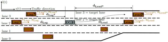
Figure 1.
Vehicles involved in a discretionary lane-change maneuver and definition of relevant variables. (*) denotes that the quantity refers to the surrounding vehicle in the target lane. Figure adapted from [41].
To ensure a minimum safety margin during lane changes, safety distances are defined for both leading and lag vehicles on the target lane. These are computed based on the respective vehicle’s velocity or , a minimum time gap , and a constant clearance term that accounts for standstill spacing.
The minimum required distance to a vehicle in front on the target lane is calculated using the current velocity of the ego vehicle , combined with a time gap and an offset at standstill:
Similarly, the rearward safety distance to a vehicle approaching from behind in the target lane is computed using the velocity of the lag vehicle , a time gap , and the clearance minimum at standstill:
Reference values for the time gap and the distance can be found in the International Standard ISO 15622, which defines specifications for adaptive cruise control (ACC) systems. To evaluate whether a safe lane change is possible, the available space both in front of and behind the ego vehicle in the target lane must be assessed. The analysis distinguishes between four distinct situations, depending on the presence and position of surrounding vehicles relative to the ego vehicle’s current state. If no relevant lead or lag vehicle is detected, the respective case is disregarded. The first two cases address the rearward environment, focusing on potential following vehicles in the target lane that may pose a conflict when changing lane.
Case 1:
In situations where the ego vehicle is traveling at a higher speed than a vehicle approaching from behind on the adjacent lane (see Figure 2), it must maintain at least the predefined safety distance (as defined in Equation (8)) before initiating a lane change. If the actual gap falls below this threshold, the lane change is considered unsafe and must be postponed.
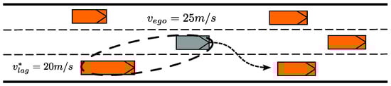
Figure 2.
Illustration of case 1.
Case 2:
If the lag vehicle in the target lane is moving at a higher speed than the ego vehicle (see Figure 3), a predictive comparison of both vehicles’ positions during the expected duration of the lane change must be conducted. This comparison ensures that a minimum safety buffer is maintained throughout the maneuver.
with as the distance between the ego and the lag vehicle. The comparison of and yields the following equation, which has to be true for safe lane-change maneuvers:
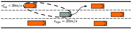
Figure 3.
Illustration of case 2.
Equation (11) considers the acceleration of the ego vehicle and the deceleration of the lag vehicle in the target lane . This formulation takes into account both the acceleration capabilities of the ego vehicle and the assumed deceleration behavior of the lag vehicle, denoted as , which reflects the maximum deceleration the lag vehicle is expected or permitted to apply in cooperative situations. The value of this accepted deceleration is critical from both a safety and traffic flow perspective. It directly influences how assertively an AV can merge with flowing traffic. The selection of this parameter is context-dependent and can vary with the urgency of the maneuver and the location on the road. For example, merging from an on-ramp typically allows for greater deceleration values from following vehicles than a standard overtaking maneuver. Moreover, this parameter also plays an important role in enabling cooperative behaviors from vehicles already on the main carriageway, especially in the vicinity of merging zones. As such, its systematic evaluation was a focal point in the use-case scenarios presented in this study.
The subsequent two cases focus on situations involving vehicles ahead of the ego vehicle in the target lane.
Case 3:
In analogy to Case 1, a minimum distance to the lead vehicle in the neighboring lane, based on Equation (7), must be ensured whenever the ego vehicle’s speed is lower than that of the vehicle ahead (see Figure 4).
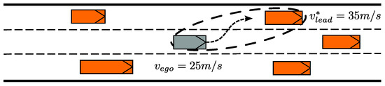
Figure 4.
Illustration of case 3.
Case 4:
If the ego vehicle is travelling faster than a lead vehicle in the adjacent lane (see Figure 5), a safe lane change can be evaluated using a similar approach to that described in case 3.
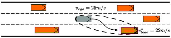
Figure 5.
Illustration of case 4.
The assessment is performed in two steps: first, the distance each vehicle is expected to cover during the lane-change period is determined; second, these distances are compared to verify whether the safety condition is fulfilled. For this case, a constant velocity of the lead vehicle is assumed.
with as the distance between the ego and the lead vehicle on the target lane. This yields the following equation, which has to be true for a safe lane-change maneuver:
In this formulation, represents the maximum deceleration the ego vehicle is allowed to apply in response to a slower vehicle ahead during the lane-change maneuver.
Provided that both the front and rear gaps satisfy the respective safety conditions, the lane change is permitted. Otherwise, the ego vehicle remains in its current lane until the calculated safety criteria are fulfilled.
A minimum distance to surrounding vehicles is ensured by the system, taking into account both the preceding vehicle in the ego lane and the one in the target lane, since the ACC controller remains active during lane-change executions. The gap to following vehicles is also incorporated into the feasibility check, considering the maximum allowable deceleration of in accordance with UN Regulation No. 157. At this stage, no trajectory re-planning module is integrated for monitoring or maintaining lateral clearance to adjacent-lane vehicles.
3.2. Non-Compliant Trajectories
Automated vehicles must strictly comply with the relevant standards and regulations for automated driving tasks to meet safety and legal requirements in all traffic conditions. The standard for adaptive cruise control systems is ISO 15622, which sets limits on acceleration and deceleration to maintain a safe distance to leading vehicles. As a result, automated driving functions require large gaps for lane-change maneuvers or must decelerate immediately in merging situations to guarantee safety. This impacts traffic flow negatively and makes dense traffic situations challenging for automated vehicles. Therefore, we address this problem by introducing a new concept called non-compliant trajectories. The purpose of non-compliant trajectories, is to facilitate the merging process for automated vehicles and to maintain the traffic flow in mixed traffic situations.
Definition 1.
A trajectory is non-compliant, when the distance to a leading vehicle, based on and the clearance minimum from ISO 15622, falls below the safe distance for a certain period of time .
3.2.1. Computation of Non-Compliant Trajectories
Figure 6 shows schematically the approach to determining if a planned lane-change trajectory is compliant with the norm. Although this concept is valid for lane-change trajectories as well as for maintain-lane trajectories, the approach in this paper is demonstrated for a lane-change maneuver. First, the trajectory of the lead vehicle affected by the planned maneuver has to be predicted. In Figure 6, the predicted trajectory of the lead vehicle on the target lane is highlighted in blue. For the prediction of , the velocity of the lead vehicle is assumed to be constant during the lane-change maneuver of the ego vehicle. The planned lane-change trajectory of the ego vehicle , highlighted in green in Figure 6, is calculated by the ego vehicle’s trajectory-planning module. Then, , the difference between the distances traveled by both vehicles in each time step, is calculated. represents a vector containing the distance between the ego and the lead vehicle at each time step.
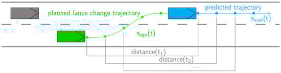
Figure 6.
Calculation of non-compliant trajectories.
All entries of the vector below the safe distance are summarized to yield a time period referred to as time below in seconds, which describes how long the planned trajectory would be below the safe distance. If the time below is between zero and a maximum allowed time , the trajectory is a non-compliant trajectory. Otherwise, it is an ordinary trajectory.
3.2.2. Following Non-Compliant Trajectories
In order to follow a non-compliant trajectory, the longitudinal controller has to be adapted to the time distance that is used for keeping a safe distance. Based on , one can also calculate a vector with new time distances for the longitudinal controller:
As long as the non-compliant status is true, the longitudinal controller has to use to maintain the distance to the lead vehicle. This also implies that the non-compliant status of a trajectory has to be verified at each time step. For instance, if the lead vehicle changes the target lane, the planned trajectory loses its non-compliant status. This verification can be performed simply by comparing the planned target velocity with the current possible velocity in the target lane at each time step.
3.3. Trajectory Evaluation
The evaluation of the generated trajectories is implemented in a separate module and includes two cost functions. There is one cost function for assessing the velocity of the trajectory, and one for the desired lane.
3.3.1. Cost Function for the Desired Velocity
The cost function for the desired velocity consists of two components. A static component, which considers the maximum velocity at the end of the planned trajectory, and a dynamic component, which assesses the velocity values along the trajectory. If the velocity at the end of the trajectory does not match the desired velocity , the cost of the static component of the velocity will be increased:
The cost of the dynamic velocity component is low if a trajectory quickly achieves the desired velocity. Therefore, the velocity values along the planned maneuver horizon are considered in the formula for the dynamic component:
The total velocity costs are given by the sum of the static part and the dynamic part, which is multiplied by an additional weight :
3.3.2. Cost Function for the Desired Lane
Due to the right-hand driving requirement in Europe, the rightmost lane is the desired lane in standard highway driving scenarios. For simulation purposes and for testing traffic management strategies, the desired lane can also be changed depending on the road segments present, for instance near on-ramps. The cost function for the desired lane is represented by a state machine that is depicted in Table 4.
Table 4.
State machine, including costs for the desired lane.
For the evaluation of the trajectory, the total costs are the sum of all cost components:
In order to vary the importance of the desired velocity or the desired lane, there are further weights, such as or , in Equation (21), to increase the impact of each component in the total cost function.
3.4. Maneuver Execution
3.4.1. Longitudinal Control
The basis for the development of the longitudinal controller was the ISO standard 15622 (third edition 2018-09). Figure 7 shows a diagram including the implemented core components of the longitudinal controller module. Basically, the longitudinal controller is a state machine with two states. One state for maintaining a safe distance to a lead vehicle, and one state for reaching the maximum desired velocity when no lead vehicle is present. Therefore, the current ego vehicle state determines which component is currently active. In accordance with the ISO standard 15622, limits for jerk and acceleration parameters are considered. The output of the longitudinal controller is the acceleration value for the next time step.
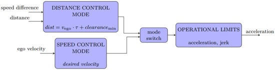
Figure 7.
State machine of longitudinal controller.
3.4.2. Lateral Control
In the microscopic simulation, the lateral dynamic and its controller for the automated driving functions are solely restricted to a simple lane-keeping function. This means that as long as the vehicle is in keep-lane mode, no specific lateral controlling mechanism is active. In the event of a lane-change maneuver, the lateral controller will be switched on and follows the coordinates of the planned trajectory to move the vehicle from the current lane to the target lane.
4. Experiment and Results
4.1. Scenario Setup
To assess the effects of the developed automated driving functions on traffic flow, we investigated a highway on-ramp segment and focused on the specific driving regulations that influence AV driving functionalities. The analyzed segment had three lanes on the main carriageway and one merging lane with a length of 250 m. Loop detectors were placed at multiple cross-sections (CS). Additional infrastructure-related properties (e.g., position of speed decision points, lane width, lane-change restrictions for varying vehicle types) were modeled as described in Leyn and Vortisch [43]. In addition, AV decision points were modeled, which allowed the AV driver behavior to be adapted. All infrastructure-related settings of the defined simulation model are illustrated in Figure 8.
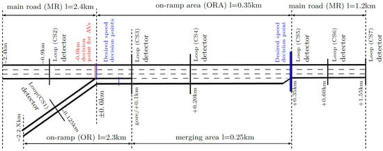
Figure 8.
Modeled on-ramp segment indicating infrastructure-related settings, the position of loop detectors, and the position of desired speed decision points.
For human-driven vehicles, we used the internal lane-change model provided in Vissim and the Wiedemann99 car-following model [30]. To calibrate the human driver behavior, a 3-step calibration process was applied utilizing single vehicle cross-section data and segment-based trajectory data according to Hofinger et al. [44]. Any adaptations in human driver behavior due to the existence of automated vehicles [45] were not considered. In addition, we obtained the desired speed distributions for passenger cars and trucks from single vehicle data from multiple cross-sections on Austrian motorways with a speed limit of 130 km/h. A truck rate of 10% was assumed. The simulation duration was set to 3 h, and every simulation scenario was simulated with five random seeds. Since we wanted to observe varying traffic states, the traffic volume was increased from 550 veh/h to 6050 veh/h in a five-minute cycle. After two thirds of the simulation time, the traffic volume reached the maximum level and was decreased again. This approach also allowed us to investigate the dissolution process of congested traffic.
In total, 13 different simulation scenarios are presented. Besides the base case, which did not consider any automated vehicles, we analyzed 12 scenarios with two different AV penetration rates and six different driving regulations, reflected by varying AV driving parameters. The AV penetration rates were defined based on an internal workshop, in which we reviewed various literature sources [46,47]. The aim of the study was to highlight potential differences between different penetration rates. However, these theoretical values should not be considered as a predicted penetration rate within a certain time span. Regarding driving regulations, we distinguished between three varying permissible following time headways. For each, it was assumed that non-compliant trajectories were either prohibited or permissible. Time headways of 0.9 s and 1.8 s corresponded to risky and conservative behaviors, respectively. As both values are rather unlikely to be defined in future driving regulations, an average time headway of 1.35 s was also investigated. An overview of the simulated scenarios can be seen in Table 5.
Table 5.
Simulation scenarios (S).
4.2. Simulation Results
Besides the overall simulation statistics, three categories of performance indicators were used to evaluate the developed AV models. First, car-following behavior analyzed the time headway and speed distributions in free-flow traffic. To distinguish between free-flow and congested traffic, the average speed and traffic density for every five-minute interval were computed and categorized based on a threshold of 70 km/h and 20 for average speed and traffic density, respectively. The data were obtained from the cross-sections shown in Figure 8.
In addition, lane change behavior was investigated. Therefore, gap acceptance characteristics and the lane change location were analyzed, focusing on merging lane changes. For gap acceptance behavior, the time headway to the lag vehicle in the target lane was computed at the time instance of starting the lane change.
Last, macroscopic traffic flow characteristics were examined by comparing the statistical indicators and spatiotemporal speed profiles of the different simulation scenarios.
The spatiotemporal speed profiles show the results of the first simulation run, and relevant averaged simulation indicators considering all simulation runs are presented in Table 6. Although congestion occurred in all simulations, deadlock situations did not happen in any simulation run.
Table 6.
Overview of mean simulation results considering all simulation runs for each scenario (S).
To investigate car-following behavior, the speed and time headway distributions are shown for three scenarios: the base case scenario A0, scenario A3, and scenario C3. The latter two scenarios took into account an AV-penetration rate of 25% and 50%, respectively. In scenarios A3 and C3, non-compliant trajectories were prohibited. All time headways shorter than 7 s were considered, as relatively high time headways have little impact on car-following behavior. The presented distributions were derived from cross-sectional data at the loop detector CS4 (see Figure 8) in free-flow traffic conditions. While the results of the base case scenario A0 in Figure 9a reflect the inherently stochastic behavior of humans, automated vehicles drive in a more homogeneous manner. This can be clearly seen in the peaks in Figure 9b,c, which correspond to the desired following time headway for AVs of 1.8 s. Moreover, the share of vehicles which maintained a time headway below 1 s decreased with increased penetration rates.
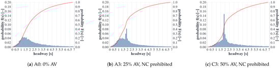
Figure 9.
Time headway distributions of scenarios A0, A3, and C3.
A similar effect can be seen in the speed distributions (Figure 10a–c). The peak between 70 and 90 km/h was due to merging vehicles in the on-ramp area, which were still in their acceleration phase and not yet driving at the desired speed. In addition, the speed distributions of scenarios A3 and C3 showed peaks at 80 km/h and 130 km/h, reflected by AVs being on the main carriageway. AVs did not exceed the maximum allowed speed (130 km/h for cars and 80 km/h for trucks) but tried to minimize travel time, which is why they drove at the maximum allowed speed in free-flow traffic situations. The higher the AV penetration rate, the higher the share of vehicles travelling at maximum allowed speed but the lower the amount of drivers driving too fast.
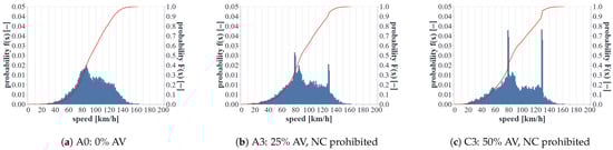
Figure 10.
Speed distributions of scenarios A0, A3, and C3.
Regarding lane-changing, the results of scenarios C3 and D3 are shown in Figure 11a–c and Figure 12b,c. Both scenarios considered an AV penetration rate of 50% and the AVs had to keep a minimum time headway of 1.8 s. In scenario C3, non-compliant trajectories were prohibited, whereas AVs were allowed to reduce the time headway () to 1.0 s for a maximum duration () of 5 s in scenario D3.
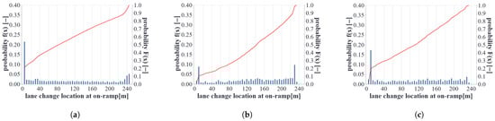
Figure 11.
Lane change location distribution of scenarios C3 and D3. (a) C3: LC location of human drivers; (b) C3: 50% AV, NC prohibited LC location of AVs; (c) D3: 50% AV, NC permitted LC location of AVs.
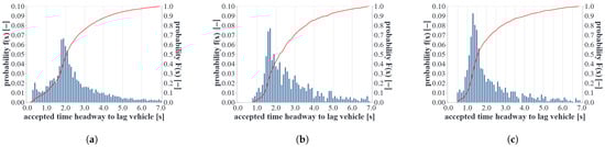
Figure 12.
Gap acceptance distribution of scenarios C3 and D3. (a) C3: Gap acceptance human drivers; (b) C3: 50% AV, NC prohibited gap acceptance AVs; (c) D3: 50% AV, NC permitted gap acceptance AVs.
The focus lay on the mandatory merging lane changes performed by the human-driven and automated vehicles in the on-ramp area, which allowed a comparison between the Vissim internal lane-change model and the developed automated driving functions. Both free and congested traffic states were considered in the derived result data. First, we analyzed the lane change location indicated by the on-ramp position where a lane-change maneuver started. The histograms and cumulative distribution functions are shown in Figure 11a–c. The x-axis shows the lane change location, ranging from 0 to 250 m, which represents the position of the gore and the end of the acceleration lane, respectively. The gore is the location at which the merging area begins and vehicles are allowed to merge into the main road (see Figure 8). Figure 11a shows the distribution of the lane change location for all human-driven vehicles controlled by Vissim. It can be seen that more than 20% of all vehicles performed the lane change at the very beginning of the acceleration lane. In comparison, the results for AVs in Figure 11b showed that almost 10% of all AVs failed to perform a lane change before the end of the acceleration lane. These AVs most likely had to stop at the end of the acceleration lane, which is undesirable since stationary vehicles can be a safety risk and it is rather difficult for a stationary vehicle to find a suitable time gap in the target lane from a standstill. These situations can be prevented if AVs are allowed to execute non-compliant trajectories, which can be seen in Figure 11c. In this case, 18% of all AVs found a suitable gap in the target lane at the very beginning of the acceleration lane. Less than 5% did not manage to merge into the main carriageway, which is a substantial reduction compared with scenario C3.
In addition, differences can be observed regarding the gap acceptance behavior in Figure 12a–c, which also explains the improved merging behavior of AVs when the non-compliant mode was permitted. The distribution in Figure 12a for human-driven vehicles shows a small peak at very low time headways. Further analysis revealed that these low headways usually occurred in situations when the lag vehicle in the target lane was a rather slow vehicle (e.g., a truck). These low time headways cannot be observed when analyzing the gap acceptance behavior of the developed automated driving functions, as a safety distance to surrounding vehicles was considered within the AV lane change model.
However, a clear shift towards smaller accepted time gaps was visible when AVs were allowed to execute non-compliant trajectories, which is the case when comparing the results from scenario C3 and D3 (see Figure 12b,c).
To analyze the impact on traffic flow, spatiotemporal speed profiles are presented for varying penetration rates and different AV driving regulations (Figure 13, Figure 14 and Figure 15). The distance before and after the on-ramp area is shown on the x-axis. The color indicates the observed average speed in space and time with a resolution of 25 m and 30 s, derived from the simulated trajectory data. The red colored areas indicate congested traffic. It can be seen that free-flow traffic was faster on the main road compared with the on-ramp link. As described in Leyn and Vortisch [43], the speed on the on-ramp link usually decreases slightly before the on-ramp area, due to increased road curvature. Therefore, the desired speed was slightly lowered 200 m before the on-ramp area, which is indicated in orange.
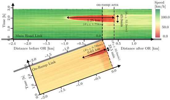
Figure 13.
Spatiotemporal speed profile of scenario A0 (Base case).
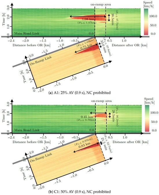
Figure 14.
Spatiotemporal speed profiles for AV penetration rates of (a) 25% and (b) 50%.
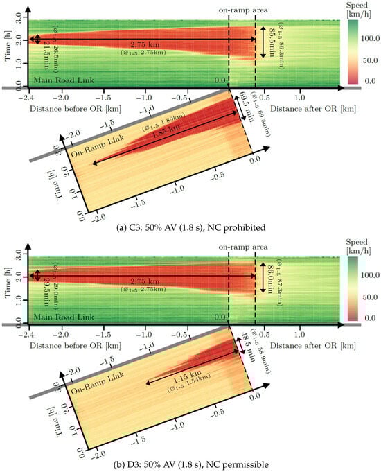
Figure 15.
Spatiotemporal speed profiles for AV penetration rates of (a) 25% and (b) 50%.
Since the traffic volume decreased after two thirds of the simulation time, the dissolution of congestion can also be observed. For the base case scenario (see Figure 13), congested traffic lasted for 43.0 and 23.5 min on the main road link and the on-ramp link, respectively. Figure 14 presents the spatiotemporal speed profiles of scenario A1 and C1. In both cases, non-compliant trajectories were prohibited and the desired time headway was set to 0.9s, which corresponds to rather risky behavior. While the AV penetration rate was set to 25% in scenario A1, scenario C1 considered an AV penetration rate of 50%. The results show that congestion was reduced on the main road if the AV penetration rates were increased. It needs to be mentioned that this was not the case if the desired time headway was set to a higher level, as shown by the results in Table 6. Moreover, congestion was not reduced at the on-ramp link when comparing the results with the base case scenario A0 in Figure 13. Increasing the AV penetration rate from 25% to 50% increased the maximum congestion length from 0.75 km to 0.83 km. In scenario C1, congestion on the on-ramp area started to emerge much later than in scenario A1. This led to a shorter time period of congested traffic on the on-ramp link.
Next, we focus on the spatiotemporal speed profiles for scenarios C3 and D3, shown in Figure 15. Both scenarios were simulated with an AV penetration rate of 50% and the desired time headway was set to 1.8 s. In scenario C3, non-compliant mode was prohibited, while it was allowed in scenario D3. First, when comparing Figure 14b and Figure 15a, it can be seen that congestion increased drastically if the AVs’ desired time headway was increased from 0.9 s to 1.8 s. Additionally, the comparison of scenarios C3 and D3 shows that only minor differences could be observed on the main road. In both scenarios, the network was fully congested. In scenario C3, this was the case for a duration of 21.5 min. Allowing AVs to execute non-compliant trajectories prolonged this state by nine minutes. However, the overall duration of congestion in the on-ramp area did not change substantially. While the on-ramp area of the main road was congested for 85.5 min in scenario C3, this value increased slightly to 86.0 min in scenario D3. At the same time, major differences can be observed at the on-ramp link as it was possible to reduce congestion significantly when AVs were allowed to execute non-compliant trajectories. On the on-ramp link, the maximum congestion length was 1.85 km in scenario C3. This was reduced by 40% to 1.15 km in scenario D3.
These results clearly demonstrate that the non-compliant mode facilitated merging maneuvers for AVs, which positively impacted the overall traffic flow. Furthermore, the number of vehicles stopping at the end of the on-ramp link was substantially reduced when the AVs operated in non-compliant mode—a finding that is also highly relevant from a safety perspective. However, it is acknowledged that a detailed safety assessment would require further analysis. The following section discusses these results in more detail and compares them with findings from previous studies.
5. Discussion
The analyses presented in the previous results section revealed key insights, which are discussed in the following. Overall, the findings underscore the importance of implementing a dedicated framework for non-compliant AV behavior. We observed that AVs had difficulties performing a merging lane change from the on-ramp towards the main road in dense traffic, particularly if the minimum time gap was set to a higher level (i.e., ). This was also found in the research by Fang et al. [25], which showed that low level AVs (i.e., SAE L3) have difficulties executing mandatory lane changes, as they require much larger time gaps than human drivers.
Permitting non-compliant behavior led to less congestion at the on-ramp link. The total duration of congested traffic was reduced by 21 min if AVs () were allowed to execute non-compliant trajectories. At the same time congestion on the main road was only minimally extended, and overall delays were reduced.
In general, we observed differences in the spatiotemporal occurrence of congestion for varying desired time headway parameters. Compared with the base case without any AVs, congestion was reduced when the desired time headway was set to 0.9 s. When was set to 1.35 s, congestion was prolonged at low penetration rates, while it was slightly reduced at higher penetration rates. Further increasing the desired time headway towards 1.8s substantially extended congested traffic, which led to an increase in travel time of up to 42.3%. Such a pattern was also found in previous studies. In the study by Postigo et al. [11], a two-lane motorway including an on-ramp and an off-ramp was simulated. Their results showed that traffic capacity was increased from 3650 veh/h in the base case scenario without any AVs up to 4200 veh/h when considering an AV penetration rate of 60% and a desired time headway of 0.9s. However, at the same penetration rate, the traffic capacity was reduced to 3300 veh/h when the desired time headway for AVs was increased to 1.5 s. In the simulation study by Li et al. [24], the car-following behavior of AVs was calibrated and modeled rather cautiously, as they defined the desired time headway parameter as 1.52 s. They performed extensive sensitivity analyses for varying parameters. Their simulation results showed that the maximum traffic volume fluctuated as the AV penetration rate increased. Maximum traffic volume decreased at low penetration rates but a minimal increase was observed at a penetration rate of 50%. They argued that improved cooperation among AVs, which was integrated into their AV behavior models, led to an increased maximum traffic volume. We observed a pattern like this for the scenario where we set equal to 1.35 s. However, further increasing the desired time headway would have most likely led to a continuous degradation of traffic flow characteristics. Hence, it would be interesting to analyze and model the cooperative behavior of AVs in more detail and investigate the resulting effects on traffic flow.
6. Conclusions
This study presented newly developed automated driving functions integrated into the microscopic traffic simulation software PTV Vissim.
Central to this work was the implementation of a non-compliant behavior framework for AVs, enabling them to temporarily reduce desired time headways in dense traffic conditions. The driving functions included trajectory planning and evaluation modules, as well as lateral and longitudinal controllers. They support on-ramp and off-ramp strategies and can dynamically adapt behavior at predefined AV decision points, making them a flexible tool for evaluating traffic management strategies.
A simulation study with 13 scenarios demonstrated that enabling AVs to operate in a non-compliant mode improved the traffic flow at on-ramps. Allowing a non-compliant mode facilitated AV lane changing behavior in dense traffic, alleviated congestion, and reduced the number of vehicles stopping at the end of the on-ramp—outcomes that are also relevant from a safety perspective. Since the safety assessments in this study were limited to gap acceptance and headway analysis, more comprehensive evaluations using metrics such as Time-To-Collision or Post-Encroachment-Time are required and planned as future work. Another important direction for future research is the re-planning of trajectories during aborted maneuvers, which was not covered in the current model. Despite this, the developed AV driving functions offer a strong foundation for simulating a wide range of traffic conditions, from free flow to congestion, and for exploring new strategies in mixed traffic.
Most importantly, this study provides guidance for regulatory development. Current legal frameworks, such as UN Regulation 157, require strict compliance with minimum time gaps. The concept of non-compliant trajectories introduced here offers a potential extension to these rules. Our results suggest that allowing controlled, explicitly defined exceptions in specific situations, such as on-ramp merging, can improve traffic performance. This regulatory flexibility would enable AVs to behave more contextually and efficiently, much like experienced human drivers.
Author Contributions
M.M.-R.: Writing–Original Draft, Conceptualization, Methodology, Software, Data curation F.H.: Writing–Original Draft, Conceptualization, Methodology, Formal analysis, Visualization, Data curation M.H.: Writing—Review and Editing, Methodology, Validation M.F.: Writing—Review and Editing, Methodology, Supervision, Funding acquisition. All authors have read and agreed to the published version of the manuscript.
Funding
This study was conducted within the project Symul8 (FFG, Austrian Research Promotion Agency, Grant No.: 882127).
Institutional Review Board Statement
Not applicable.
Informed Consent Statement
Not applicable.
Data Availability Statement
Cross-sectional data provided by the Austrian motorway operator ASFINAG was used to calibrate human driver behaviour. The data presented in this study are available on request from the corresponding author. The data are not publicly available due to privacy constraints, this data is subject to access restrictions.
Acknowledgments
The project was funded by the program “Mobilität der Zukunft” of the Austrian Federal Ministry for Climate Action (BMK). Financial support by the road authorities ASFINAG (AT), BAST (GER), and ASTRA (CH) is gratefully acknowledged. The publication was written at Virtual Vehicle Research GmbH in Graz and partially funded within the COMET K2 Competence Centers for Excellent Technologies from the Austrian Federal Ministry for Climate Action (BMK), the Austrian Federal Ministry for Labour and Economy (BMAW), the Province of Styria (Dept. 12) and the Styrian Business Promotion Agency (SFG). The Austrian Research Promotion Agency (FFG) has been authorized for program management. The document details some of the research output of the project. However, it does not express the view or opinions of the involved road authorities.
Conflicts of Interest
The authors declare that they have no known competing financial interests or personal relationships that could have appeared to influence the work reported in this paper.
References
- Azam, M.; Hassan, S.A.; Che Puan, O. Autonomous Vehicles in Mixed Traffic Conditions—A Bibliometric Analysis. Sustainability 2022, 14, 10743. [Google Scholar] [CrossRef]
- Chang, X.; Zhang, X.; Li, H.; Wang, C.; Liu, Z. A Survey on Mixed Traffic Flow Characteristics in Connected Vehicle Environments. Sustainability 2022, 14, 7629. [Google Scholar] [CrossRef]
- United Nations Economic and Social Council. Proposal for the 01 series of amendments to UN Regulation No. 157 (Automated Lane Keeping Systems). ECE/TRANS/WP.29/2022/59/Rev.1. 2022. Available online: https://unece.org/sites/default/files/2025-03/ECE_TRANS_WP.29_2022_59_Rev.1e.pdf (accessed on 7 July 2025).
- Mattas, K.; Albano, G.; Donà, R.; Galassi, M.C.; Suarez-Bertoa, R.; Vass, S.; Ciuffo, B. Driver models for the definition of safety requirements of automated vehicles in international regulations. Application to motorway driving conditions. Accid. Anal. Prev. 2022, 174, 106743. [Google Scholar] [CrossRef]
- Farah, H.; Postigo, I.; Reddy, N.; Dong, Y.; Rydergren, C.; Raju, N.; Olstam, J. Modeling Automated Driving in Microscopic Traffic Simulations for Traffic Performance Evaluations: Aspects to Consider and State of the Practice. IEEE Trans. Intell. Transp. Syst. 2022, 24, 6558–6574. [Google Scholar] [CrossRef]
- Olstam, J.; Johansson, F.; Alessandrini, A.; Sukennik, P.; Lohmiller, J.; Friedrich, M. An Approach for Handling Uncertainties Related to Behaviour and Vehicle Mixes in Traffic Simulation Experiments with Automated Vehicles. J. Adv. Transp. 2020, 2020, 1–17. [Google Scholar] [CrossRef]
- Ahmed, H.U.; Huang, Y.; Lu, P. A Review of Car-Following Models and Modeling Tools for Human and Autonomous-Ready Driving Behaviors in Micro-Simulation. Smart Cities 2021, 4, 314–335. [Google Scholar] [CrossRef]
- Do, W.; Rouhani, O.M.; Miranda-Moreno, L. Simulation-Based Connected and Automated Vehicle Models on Highway Sections: A Literature Review. J. Adv. Transp. 2019, 2019, 9343705. [Google Scholar] [CrossRef]
- Al-Turki, M.; Ratrout, N.T.; Rahman, S.M.; Reza, I. Impacts of Autonomous Vehicles on Traffic Flow Characteristics under Mixed Traffic Environment: Future Perspectives. Sustainability 2021, 13, 11052. [Google Scholar] [CrossRef]
- Wiedemann, R. Simulation des Straßenverkehrsflusses; Schriftenreihe des Instituts für Verkehrswesen der Universität Karlsruhe: Karlsruhe, Germany, 1974. [Google Scholar]
- Postigo, I.; Olstam, J.; Rydergren, C. Effects on Traffic Performance Due to Heterogeneity of Automated Vehicles on Motorways: A Microscopic Simulation Study. In Proceedings of the 7th International Conference on Vehicle Technology and Intelligent Transport Systems, Online, 28–30 April 2021; pp. 142–151. [Google Scholar] [CrossRef]
- Schakel, W.J.; van Arem, B.; Netten, B.D. Effects of Cooperative Adaptive Cruise Control on traffic flow stability. In Proceedings of the 13th International IEEE Conference on Intelligent Transportation Systems, Madeira, Portugal, 19–22 September 2010; pp. 759–764. [Google Scholar] [CrossRef]
- Schakel, W.J.; Knoop, V.L.; van Arem, B. Integrated Lane Change Model with Relaxation and Synchronization. Transp. Res. Rec. J. Transp. Res. Board 2012, 2316, 47–57. [Google Scholar] [CrossRef]
- Calvert, S.C.; Schakel, W.J.; van Lint, J.W.C. Will Automated Vehicles Negatively Impact Traffic Flow? J. Adv. Transp. 2017, 2017, 1–17. [Google Scholar] [CrossRef]
- Treiber, M.; Hennecke, A.; Helbing, D. Congested traffic states in empirical observations and microscopic simulations. Phys. Rev. E 2000, 62, 1805–1824. [Google Scholar] [CrossRef] [PubMed]
- Erdmann, J. SUMO’s Lane-Changing Model. In Modeling Mobility with Open Data; Behrisch, M., Weber, M., Eds.; Lecture Notes in Mobility; Springer International Publishing: Cham, Switzerland, 2015; pp. 105–123. [Google Scholar] [CrossRef]
- Kavas-Torris, O.; Lackey, N.; Guvenc, L. Simulating the Effect of Autonomous Vehicles on Roadway Mobility in a Microscopic Traffic Simulator. Int. J. Automot. Technol. 2021, 22, 713–733. [Google Scholar] [CrossRef]
- Gipps, P.G. A behavioural car-following model for computer simulation. Transp. Res. Part B Methodol. 1981, 15, 105–111. [Google Scholar] [CrossRef]
- Miqdady, T.; de Ona, R.; Casas, J.; de Ona, J. Studying Traffic Safety During the Transition Period Between Manual Driving and Autonomous Driving: A Simulation-Based Approach. IEEE Trans. Intell. Transp. Syst. 2023, 24, 6690–6710. [Google Scholar] [CrossRef]
- Milanés, V.; Shladover, S.E. Modeling cooperative and autonomous adaptive cruise control dynamic responses using experimental data. Transp. Res. Part C Emerg. Technol. 2014, 48, 285–300. [Google Scholar] [CrossRef]
- Elmorshedy, L.; Abdulhai, B.; Kamel, I. Quantitative Evaluation of the Impacts of the Time Headway of Adaptive Cruise Control Systems on Congested Urban Freeways Using Different Car Following Models and Early Control Results. IEEE Open J. Intell. Transp. Syst. 2022, 3, 288–301. [Google Scholar] [CrossRef]
- Zhi, Y.; Zhang, Z.; Zhou, W.; Hou, D.; Zhang, J. Evaluation of Mixed Traffic Flow Efficiency and Safety on Hard-Shoulder-Running Freeways. Appl. Sci. 2024, 14, 11137. [Google Scholar] [CrossRef]
- Porfyri, K.N.; Mintsis, E.; Mitsakis, E. Assessment of ACC and CACC Systems Using SUMO; EasyChair, EPiC Series in Engineering; EPIC Engineering: Heber City, UT, USA, 2018; pp. 82–93. [Google Scholar] [CrossRef]
- Li, Q.; Li, X.; Huang, Z.; Halkias, J.; McHale, G.; James, R. Simulation of mixed traffic with cooperative lane changes. Comput.-Aided Civ. Infrastruct. Eng. 2021, 37, 1978–1996. [Google Scholar] [CrossRef]
- Fang, X.; Li, H.; Tettamanti, T.; Eichberger, A.; Fellendorf, M. Effects of Automated Vehicle Models at the Mixed Traffic Situation on a Motorway Scenario. Energies 2022, 15, 2008. [Google Scholar] [CrossRef]
- Li, H.; Ju, Y. Microscopic Simulation of Heterogeneous Traffic Flow on Multi-Lane Ring Roads and Highways. Appl. Sci. 2025, 15, 1453. [Google Scholar] [CrossRef]
- Lee, S.; Jeong, E.; Oh, M.; Oh, C. Driving aggressiveness management policy to enhance the performance of mixed traffic conditions in automated driving environments. Transp. Res. Part A Policy Pract. 2019, 121, 136–146. [Google Scholar] [CrossRef]
- Khattak, Z.H.; Smith, B.L.; Park, H.; Fontaine, M.D. Cooperative lane control application for fully connected and automated vehicles at multilane freeways. Transp. Res. Part C Emerg. Technol. 2020, 111, 294–317. [Google Scholar] [CrossRef]
- Han, Y.; Ahn, S. Variable Speed Release (VSR): Speed Control to Increase Bottleneck Capacity. IEEE Trans. Intell. Transp. Syst. 2020, 21, 298–307. [Google Scholar] [CrossRef]
- Fellendorf, M.; Vortisch, P. Microscopic Traffic Flow Simulator VISSIM. In Fundamentals of Traffic Simulation; Barceló, J., Ed.; Springer: New York, NY, USA, 2010; Volume 145, pp. 63–93. [Google Scholar] [CrossRef]
- Kesting, A.; Treiber, M.; Schönhof, M.; Helbing, D. Extending Adaptive Cruise Control to Adaptive Driving Strategies. Transp. Res. Rec. J. Transp. Res. Board 2007, 2000, 16–24. [Google Scholar] [CrossRef]
- Li, X.; Liu, Z.; Li, M.; Liu, Y.; Wang, C.; Ma, X.; Liang, Y. Research on the weaving area capacity of freeways under man–machine mixed traffic flow. Phys. A Stat. Mech. Its Appl. 2023, 625, 129040. [Google Scholar] [CrossRef]
- SAE-Society of Automotive Engineers. Taxonomy and Definitions for Terms Related to Driving Automation Systems for On-Road Motor Vehicles. 2021. Available online: https://saemobilus.sae.org/standards/j3016_202104-taxonomy-definitions-terms-related-driving-automation-systems-road-motor-vehicles (accessed on 7 July 2025).
- ISO 15622; Intelligent Transport Systems—Adaptive Cruise Control Systems—Performance Requirements and Test Procedures. ISO: Geneva, Switzerland, 2018.
- Katrakazas, C.; Quddus, M.A.; Chen, W.; Deka, L. Real-time motion planning methods for autonomous on-road driving: State-of-the-art and future research directions. Transp. Res. Part C-Emerg. Technol. 2015, 60, 416–442. [Google Scholar]
- Dixit, S.; Fallah, S.; Montanaro, U.; Dianati, M.; Stevens, A.; Mccullough, F.; Mouzakitis, A. Trajectory planning and tracking for autonomous overtaking: State-of-the-art and future prospects. Annu. Rev. Control 2018, 45, 76–86. [Google Scholar] [CrossRef]
- Paden, B.; Čáp, M.; Yong, S.; Yershov, D.; Frazzoli, E. A survey of motion planning and control techniques for self-driving urban vehicles. IEEE Trans. Intell. Veh. 2016, 1, 33–55. [Google Scholar] [CrossRef]
- Schwarting, W.; Alonso-Mora, J.; Rus, D. Planning and Decision-Making for Autonomous Vehicles. Annu. Rev. Control. Robot. Auton. Syst. 2018, 1, 187–210. [Google Scholar] [CrossRef]
- Hult, R.; Tabar, R. Path Planning for Highly Automated Vehicles. Master’s Thesis, Chalmers University of Technology, Gothenburg, Sweden, 2013. [Google Scholar]
- Rupp, A. Trajectory Planning and Formation Control for Automated Driving on Highways. Ph.D. Thesis, Graz University of Technology, Graz, Austria, 2018. [Google Scholar]
- Hofinger, F.; Mischinger-Rodziewicz, M.; Haberl, M.; Fellendorf, M. Lane Change Model for Automated Vehicles on Multi-Lane Highways in Mixed Traffic. In Proceedings of the 2023 IEEE 26th International Conference on Intelligent Transportation Systems (ITSC), Bilbao, Spain, 24–28 September 2023; pp. 2004–2009. [Google Scholar] [CrossRef]
- Choudhury, C.; Ben-Akiva, M.E.; Toledo, T.; Rao, A.; Lee, G. State Dependence in Lane Changing Models 1 PAPER: 196 State Dependence in Lane Changing Models. In Proceedings of the 17th International Symposium on Transportation and Traffic Theory, London, UK, 23–25 July 2007; Elsevier: London, UK, 2007. [Google Scholar]
- Leyn, U.; Vortisch, P. Calibrating VISSIM for the German Highway Capacity Manual. Transp. Res. Rec. J. Transp. Res. Board 2015, 2483, 74–79. [Google Scholar] [CrossRef]
- Hofinger, F.; Haberl, M.; Fellendorf, M.; Rosenkranz, P.; Mischinger, M.; Brandenburg, A.; Hoser, M. 3-step calibration process of a microscopic traffic flow simulation platform for mixed traffic scenarios. Transp. Res. Procedia 2023, 72, 1778–1785. [Google Scholar] [CrossRef]
- Jiao, Y.; Li, G.; Calvert, S.C.; van Cranenburgh, S.; van Lint, H. Beyond behavioural change: Investigating alternative explanations for shorter time headways when human drivers follow automated vehicles. Transp. Res. Part C Emerg. Technol. 2024, 164, 104673. [Google Scholar] [CrossRef]
- Hartmann, M.; Motamedidehkordi, N.; Krause, S.; Hoffmann, S.; Vortisch, P.; Busch, F. Impact of Automated Vehicles on Capacity of the German Freeway Network. In ITS World Congress 2017 Compendium of Papers; ITS World Congress: Montreal, QC, Canada, 2017. [Google Scholar]
- Lytrivis, P.; Manganiaris, S.; Tötzl, D.; Berghäuser, G.; Mischinger, M.; Rudigier, M.; Solmaz, S.; Wimmer, Y.; Pintsuk, A.; Porcuna, D.; et al. INFRAMIX Deliverable. 5.3: Evaluation, impact analysis and new safety performance criteria. 2020; Available online: https://www.inframix.eu/wp-content/uploads/INFRAMIX_D5.3_1.0-final.pdf (accessed on 7 July 2025).
Disclaimer/Publisher’s Note: The statements, opinions and data contained in all publications are solely those of the individual author(s) and contributor(s) and not of MDPI and/or the editor(s). MDPI and/or the editor(s) disclaim responsibility for any injury to people or property resulting from any ideas, methods, instructions or products referred to in the content. |
© 2025 by the authors. Licensee MDPI, Basel, Switzerland. This article is an open access article distributed under the terms and conditions of the Creative Commons Attribution (CC BY) license (https://creativecommons.org/licenses/by/4.0/).