
Optimization Model of Express–Local Train Schedules Under Cross-Line Operation of Suburban Railway

Abstract
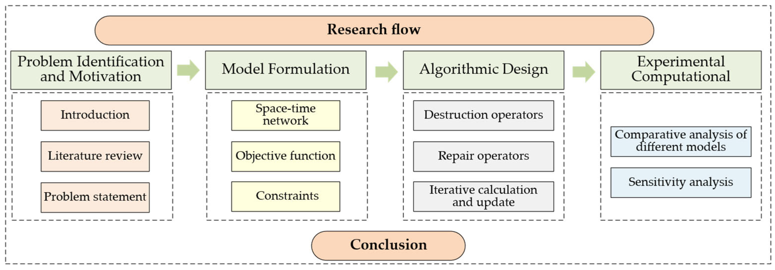
1. Introduction
2. Literature Review
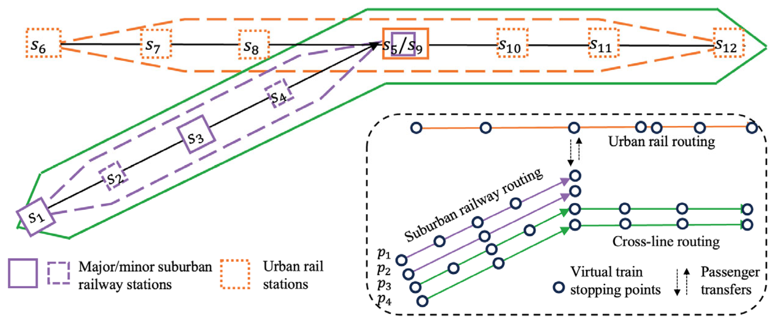
3. Problem Statement
- (1)
- indicates that the suburban train adopts stop-and-go mode and operates only within the suburban line;
- (2)
- indicates that the suburban train adopts the station stop mode based on cross-line to the common line section of the urban rail transit line;
- (3)
- denotes suburban trains using a large stop-and-go mode, skipping some small stops and operating only within the suburban line;
- (4)
- indicates that the suburban train adopts the large station express train mode based on the cross-line to the common line section of the urban rail transit line.
3.1. Basic Assumption
3.2. Symbol Definition
- if a suburban railway train that takes service timetable and has first departure time is put into service;
- otherwise, ;
- if the suburban railway train travel arc is covered by a suburban railway train that adopts service timetable and has first station departure time ;
- otherwise, ;
- if a train stops at station in a suburban railway train service plan ;
- otherwise, ;
4. Space–Time Network Construction
5. Mathematical Model
5.1. Objective Function
5.2. Constraints
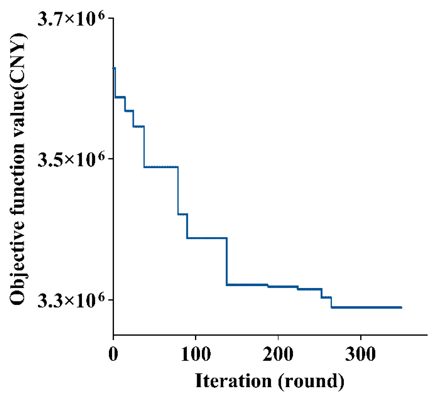
6. Algorithmic Design
- 1.
- Train Removal-Based Destruction Operators:
- (a)
- Randomly select a train from the current timetable and remove it.
- (b)
- Calculate the departure intervals between neighboring trains at each station, and remove the train whose deletion results in the smallest overall interval during operating hours.
- (c)
- For each train with service plan p and first-station departure time t, evaluate the number of passenger boardings at each station s. Remove the train with the lowest total number of passenger boardings.
- 2.
- Service Plan-Based Destruction Operators:
- (a)
- Randomly change a train’s service pattern from a local train to an express train.
- (b)
- For each express train, count the total number of boardings at small stations. Identify the local train with the lowest small-station boardings and change it to an express train.
- (c)
- Randomly change a cross-line train into a non-cross-line train.
- (d)
- Identify the cross-line train with the lowest number of passengers traveling to segments shared with urban rail lines and convert it into a non-cross-line train.
- 1.
- Train Reinsertion-Based Repair Operators:
- (a)
- Randomly select a train and reinsert it into the current timetable.
- (b)
- Compute the departure intervals at each station, identify the time slot with the largest interval across all stations, and insert a train at that point.
- (c)
- Identify stations with high passenger backlogs and insert a train into the timetable, with the specific train selected randomly.
- 2.
- Service Plan-Based Repair Operators:
- (a)
- Randomly convert an express train back to a local train.
- (b)
- For each local train, identify small stations with severe passenger backlogs, and convert the associated train to an express train if appropriate.
- (c)
- Randomly convert a non-cross-line train into a cross-line train.
- (d)
- Identify the non-cross-line train with the highest passenger flow destined for segments shared with urban rail lines and convert it into a cross-line train.
| Algorithm 1. E-ALNS framework. |
| Algorithmic Process |
Step 1 Input:
with roulette; ); with roulette; ); Compare the objective values of the solutions: If F( ; If ; Else evaluate using simulated annealing: ; If : ; Update operator scores: If then Else then ; Else ; Else no change; Update the weights based on the operator scores; ; If : : ; ; Step 3 Output: train_timetable, stop_plan, stoptime_plan |
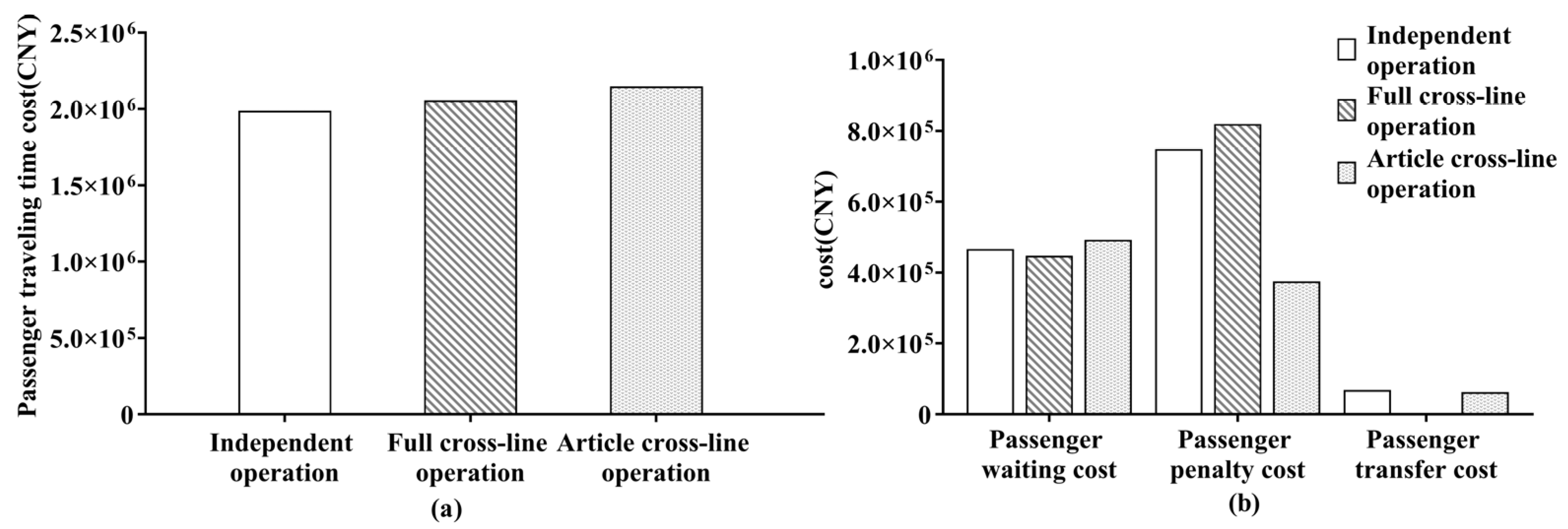
7. Computational Results
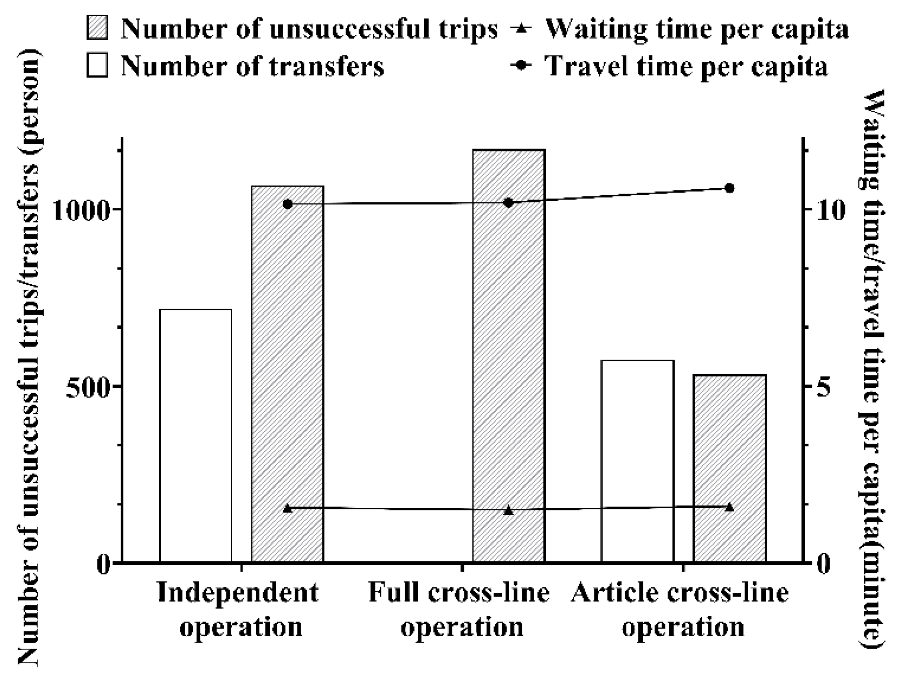
7.1. Comparative Analysis of Different Models
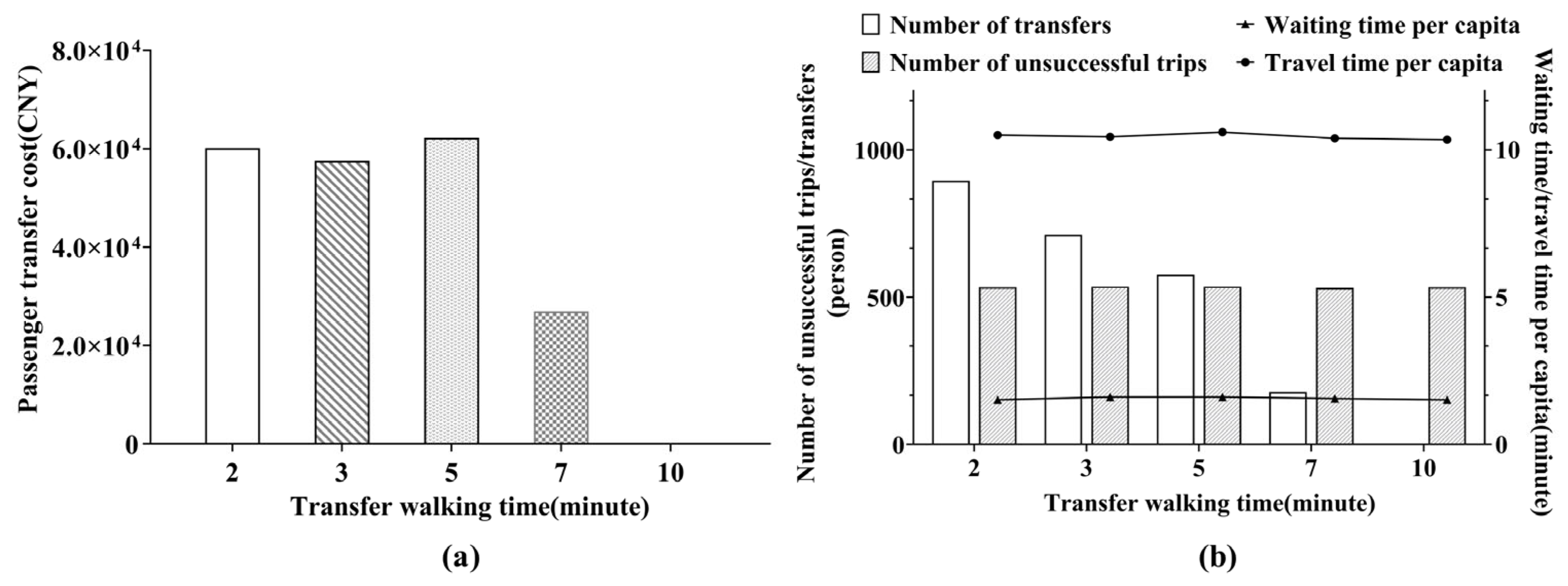
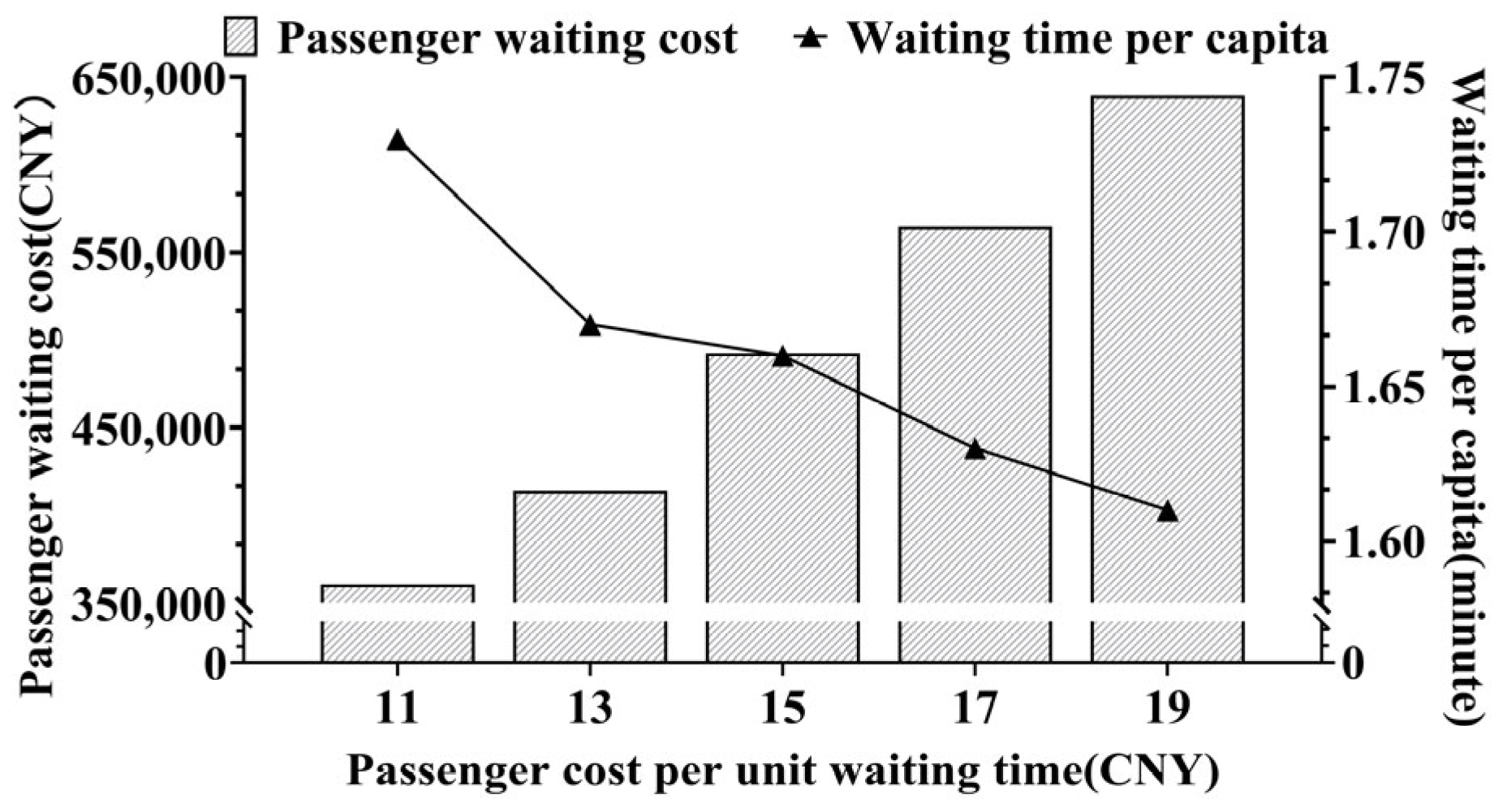
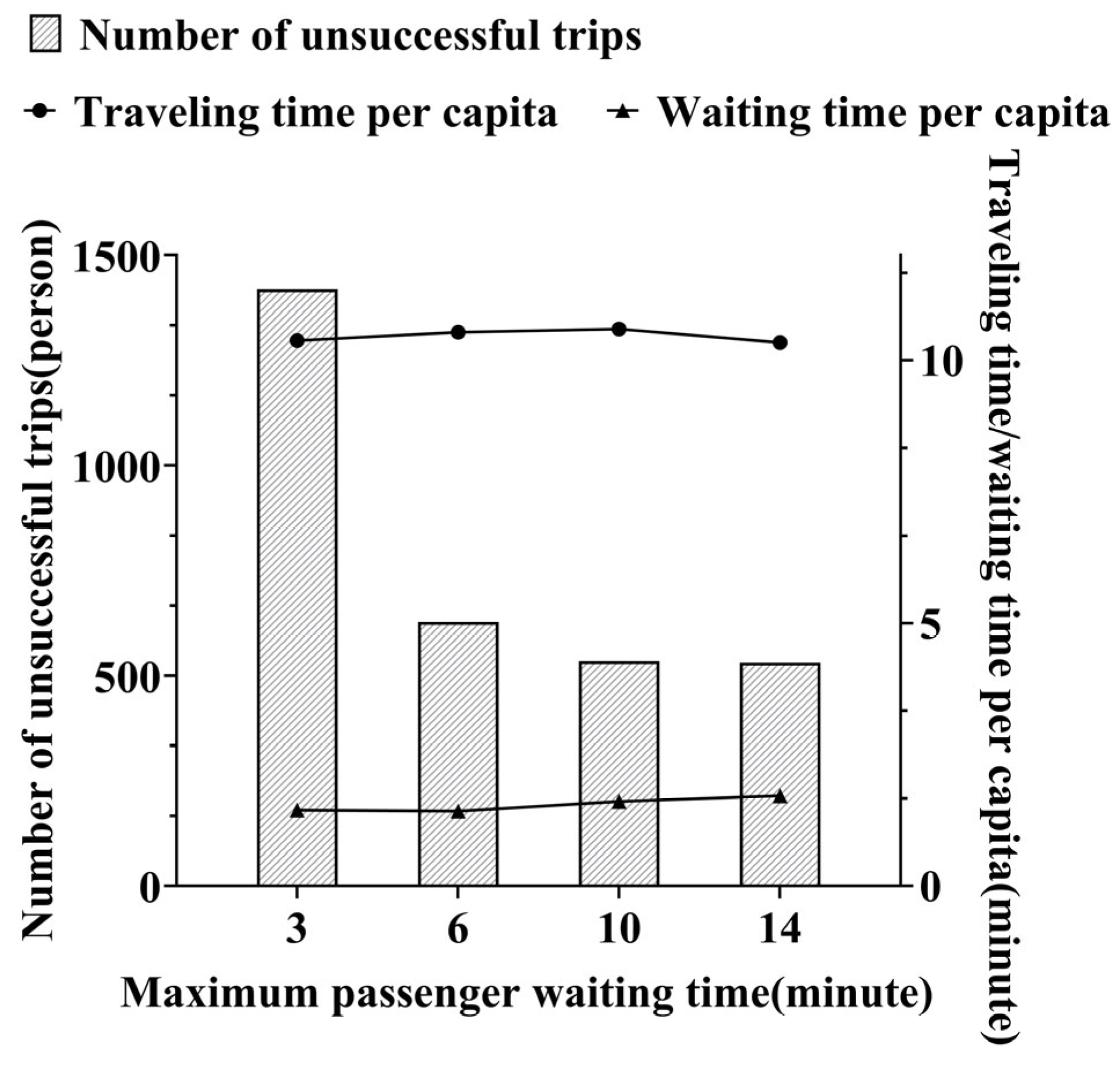
7.2. Sensitivity Analysis
8. Conclusions
Author Contributions
Funding
Institutional Review Board Statement
Informed Consent Statement
Data Availability Statement
Conflicts of Interest
References
- Ding, X.; Guan, S.; Sun, D.; Jia, L. Short Turning Pattern for Relieving Metro Congestion During Peak Hours: The Substance Coherence of Shanghai, China. Eur. Transp. Res. Rev. 2018, 10, 28. [Google Scholar] [CrossRef]
- Niu, H.; Zhou, X. Optimizing Urban Rail Timetable under Time-Dependent Demand and Oversaturated Conditions. Transp. Res. Part C 2013, 36, 212–230. [Google Scholar] [CrossRef]
- Niu, H.; Zhou, X.; Gao, R. Train Scheduling for Minimizing Passenger Waiting Time with Time-Dependent Demand and Skip-Stop Patterns: Nonlinear Integer Programming Models with Linear Constraints. Transp. Res. Part B 2015, 76, 117–135. [Google Scholar] [CrossRef]
- Shang, P.; Li, R.; Liu, Z.; Yang, L.; Wang, Y. Equity-oriented skip-stopping schedule optimization in an oversaturated urban rail transit network. Transp. Res. Part C 2018, 89, 321–343. [Google Scholar] [CrossRef]
- Li, Z.; Mao, B.; Bai, Y.; Chen, Y. Integrated Optimization of Train Stop Planning and Scheduling on Metro Lines with Express/Local Mode. IEEE Access 2019, 7, 88534–88546. [Google Scholar] [CrossRef]
- Wong, W.C.R.; Yuen, Y.W.T.; Fung, W.K.; Leung, J.M.Y. Optimizing Timetable Synchronization for Rail Mass Transit. Transp. Sci. 2008, 42, 57–69. [Google Scholar] [CrossRef]
- Yin, J.; Yang, L.; Tang, T.; Gao, Z. Dynamic Passenger Demand Oriented Metro Train Scheduling with Energy-Efficiency and Waiting Time Minimization: Mixed-Integer Linear Programming Approaches. Transp. Res. Part B 2017, 97, 182–213. [Google Scholar] [CrossRef]
- Barrena, E.; Canca, D.; Coelho, L.C.; Laporte, G. Exact Formulations and Algorithm for the Train Timetabling Problem with Dynamic Demand. Comput. Oper. Res. 2014, 44, 66–74. [Google Scholar] [CrossRef]
- Dong, X.; Li, D.; Yin, Y.; Gao, Z. Integrated Optimization of Train Stop Planning and Timetabling for Commuter Railways with an Extended Adaptive Large Neighborhood Search Metaheuristic Approach. Transp. Res. Part C 2020, 117, 102667. [Google Scholar] [CrossRef]
- Corman, F.; D’Ariano, A.; Hansen, I.A. Evaluating Disturbance Robustness of Railway Schedules. J. Intell. Transp. Syst. 2014, 18, 106–120. [Google Scholar] [CrossRef]
- Veelenturf, L.P.; Kroon, L.G.; Maróti, G. Passenger Oriented Railway Disruption Management by Adapting Timetables and Rolling Stock Schedules. Transp. Res. Part C 2017, 80, 133–147. [Google Scholar] [CrossRef]
- Gao, Y.; Kroon, L.; Schmidt, M.; Schöbel, A. Rescheduling a Metro Line in an Over-Crowded Situation after Disruptions. Transp. Res. Part B 2016, 93, 425–449. [Google Scholar] [CrossRef]
- Sun, L.; Lu, H.; Xu, Y.; Kong, D.; Shao, J. Fairness-Oriented Train Service Design for Urban Rail Transit Cross-Line Operation. Phys. A 2022, 606, 128124. [Google Scholar] [CrossRef]
- Zhu, Y.; Goverde, M.R. Railway Timetable Rescheduling with Flexible Stopping and Flexible Short-Turning during Disruptions. Transp. Res. Part B 2019, 123, 149–181. [Google Scholar] [CrossRef]
- Zhou, Y.; Yang, H.; Wang, Y.; Yan, X. Integrated Line Configuration and Frequency Determination with Passenger Path Assignment in Urban Rail Transit Networks. Transp. Res. Part B 2021, 145, 134–151. [Google Scholar] [CrossRef]
- Kurosaki, F. Through-Train Services: A Comparison between Japan and Europe. JRTR 2014, 63, 22–25. [Google Scholar]
- Yang, A.; Wang, B.; Huang, J.; Li, C. Service replanning in urban rail transit networks: Cross-line express trains for reducing the number of passenger transfers and travel time. Transp. Res. Part C 2020, 115, 102629. [Google Scholar] [CrossRef]
- Zhao, K.; Zhu, C.; Li, X.; Zhang, Y. Train Service Design for Cross-Line Operation during Peak Passenger Flow Period. IAENG Int. J. Appl. Math. 2024, 54, 1797–1806. [Google Scholar]
- Abdelhafiez, A.E.; Salama, R.M.; Shalaby, A.M. Minimizing passenger travel time in URT system adopting skip-stop strategy. J. Rail Transp. Plan. Manag. 2017, 7, 277–290. [Google Scholar] [CrossRef]
- Gao, Y.; Yang, L.; Gao, Z. Energy Consumption and Travel Time Analysis for Metro Lines with Express/Local Mode. Transp. Res. Part D 2018, 60, 7–27. [Google Scholar] [CrossRef]
- Parbo, J.; Nielsen, A.O.; Prato, G.C. Reducing Passengers’ Travel Time by Optimising Stopping Patterns in a Large-Scale Network: A Case Study in the Copenhagen Region. Transp. Res. Part A 2018, 113, 197–212. [Google Scholar] [CrossRef]
- Huang, X.; Liang, Q.; Li, S.; Wang, J. Research on Passenger Flow Assignment of Integrated Cross-Line and Skip-Stop Operation between State Railway and Suburban Railway. Appl. Sci. 2022, 12, 3617. [Google Scholar] [CrossRef]
- Mara, S.; Norcahyo, R.; Jodiawan, P.; Lusiantoro, L.; Rifai, A. A survey of adaptive large neighborhood search algorithms and applications. Comput. Oper. Res. 2022, 146, 105903. [Google Scholar] [CrossRef]
- Canca, D.; De-Los-Santos, A.; Laporte, G.; Mesa, J.A. An Adaptive Neighborhood Search Metaheuristic for the Integrated Railway Rapid Transit Network Design and Line Planning Problem. Comput. Oper. Res. 2017, 78, 1–14. [Google Scholar] [CrossRef]
- Moritz, R.; Cordeau, J.-F. Adaptive Large Neighborhood Search for Integrated Planning in Railroad Classification Yards. Transp. Res. Part B 2021, 150, 26–51. [Google Scholar]
- Zheng, H.; Sun, H.; Zhu, S.; Kang, L.; Wu, J. Air Cargo Network Planning and Scheduling Problem with Minimum Stay Time: A Matrix-Based ALNS Heuristic. Transp. Res. Part C 2023, 156, 104257. [Google Scholar] [CrossRef]


| The Value of the Objective Function | Gap | ||
|---|---|---|---|
| Gurobi | E-ALNS | ||
| 0.8 | 2,558,611 | 2,640,264 | 3.19% |
| 1.0 | 3,192,764 | 3,289,185 | 3.02% |
| 1.5 | 4,758,355 | 4,940,115 | 3.82% |
| Full Cross-Line Operation/Independent Operation | Article Cross-Line Opera-Tion/Independent Operation | |
|---|---|---|
| Ratio of objective function values | 1.02 | 0.95 |
| Ratio of train operating | 1.04 | 1.08 |
| Ratio of total passenger travel cost | 1.02 | 0.94 |
| Total passenger travel cost/train operating cost | 0.97 | 0.87 |
| Ratio of Objective Function Value to Baseline | Ratio of Train Operating Cost to Baseline | Ratio of Total Passenger Travel Cost to Baseline | |
|---|---|---|---|
| 2 | 0.99 | 0.97 | 0.99 |
| 3 | 0.99 | 1.04 | 1 |
| 5 | 1 | 1 | 1 |
| 7 | 0.98 | 1.06 | 0.98 |
| 10 | 0.98 | 1.08 | 0.97 |
| Ratio of Objective Function Value to Baseline | Ratio of Train Operating Cost to Baseline | Ratio of Total Passenger Travel Cost to Baseline | |
|---|---|---|---|
| 300 | 0.93 | 0.92 | 0.93 |
| 500 | 0.96 | 1.02 | 0.95 |
| 700 | 1 | 1 | 1 |
| 900 | 1.04 | 0.98 | 1.05 |
| 1100 | 1.07 | 1.01 | 1.07 |
| Objective function value | 3,725,174 | 3,315,659 | 3,289,185 | 3,222,923 |
| Ratio to baseline | 1.12 | 0.99 | 1 | 1.02 |
Disclaimer/Publisher’s Note: The statements, opinions and data contained in all publications are solely those of the individual author(s) and contributor(s) and not of MDPI and/or the editor(s). MDPI and/or the editor(s) disclaim responsibility for any injury to people or property resulting from any ideas, methods, instructions or products referred to in the content. |
© 2025 by the authors. Licensee MDPI, Basel, Switzerland. This article is an open access article distributed under the terms and conditions of the Creative Commons Attribution (CC BY) license (https://creativecommons.org/licenses/by/4.0/).
Share and Cite
Zhu, J.; Guo, X.; Pan, J. Optimization Model of Express–Local Train Schedules Under Cross-Line Operation of Suburban Railway. Appl. Sci. 2025, 15, 7853. https://doi.org/10.3390/app15147853
Zhu J, Guo X, Pan J. Optimization Model of Express–Local Train Schedules Under Cross-Line Operation of Suburban Railway. Applied Sciences. 2025; 15(14):7853. https://doi.org/10.3390/app15147853
Chicago/Turabian StyleZhu, Jingyi, Xin Guo, and Jianju Pan. 2025. "Optimization Model of Express–Local Train Schedules Under Cross-Line Operation of Suburban Railway" Applied Sciences 15, no. 14: 7853. https://doi.org/10.3390/app15147853
APA StyleZhu, J., Guo, X., & Pan, J. (2025). Optimization Model of Express–Local Train Schedules Under Cross-Line Operation of Suburban Railway. Applied Sciences, 15(14), 7853. https://doi.org/10.3390/app15147853