

A Data-Driven Approach for Generating Synthetic Load Profiles with GANs


Abstract
1. Introduction
- Fidelity—the synthetic data should have the same or similar data distribution as the original data;
- Flexibility—the models, generating the data, should allow for the generation of data of a particular class;
- Privacy—the generation of the data should be anonymized while keeping its integrity and distribution.
2. Materials and Methods
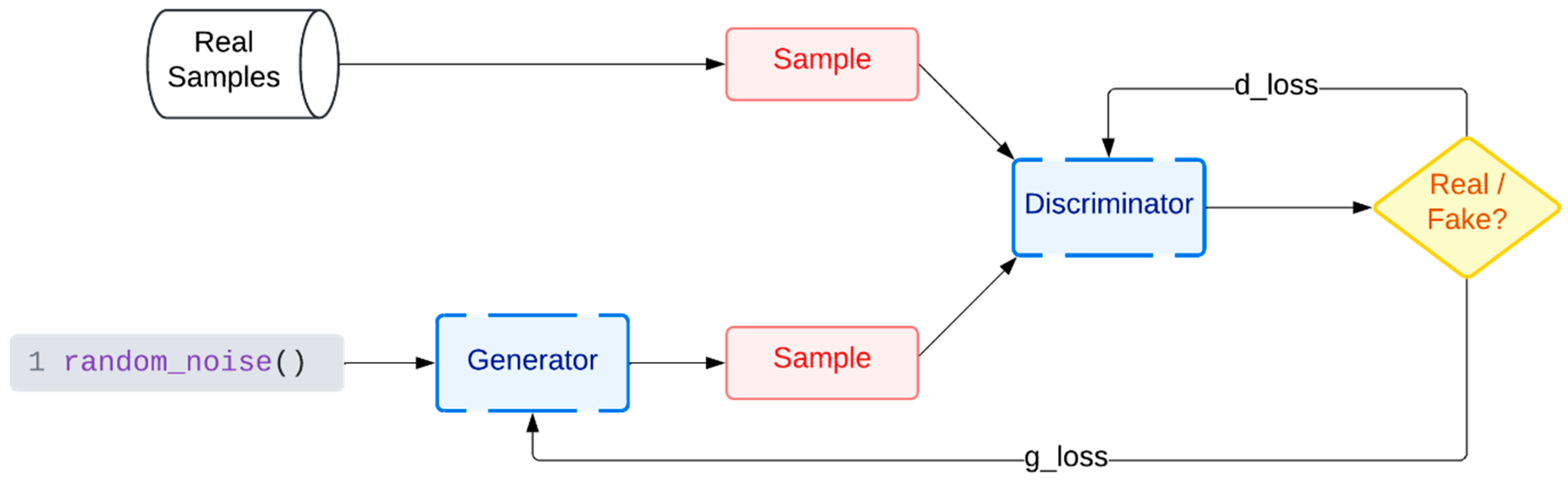
2.1. GAN Explanation and Definition
2.2. Requirements Toward the GAN-Based Synthetic Data for Electrical Load Profiles
- (1)
- Synthetic load profiles must preserve the overall shape and behavioral dynamics of real electricity consumption. This includes accurately capturing daily cycles, such as morning and evening peaks that occur in most residential buildings, as well as base load behavior during off-peak hours. For industrial facilities, the profiles may follow production-related patterns. If such patterns are not captured, the synthetic data will lack ecological validity and fail to serve its intended purpose.
- (2)
- The generated data must respect the statistical properties of the original dataset. This may include preserving the mean, variance, skewness, kurtosis, and other domain-specific features, such as load factor, energy-to-peak ratio, or hour-to-hour correlation coefficients. These properties guarantee how well synthetic data can be used to train or test load forecasting models or simulate grid scenarios. If statistical alignment is not maintained, predictive models trained on such data may produce biased or unstable results, especially in applications like smart grid control or demand response planning.
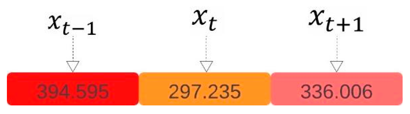
- (3)
- It is critical to maintain the temporal structure of the data. Electrical load profiles are a type of time series, and the value at a given hour (e.g., 3 PM) is not independent of the preceding hours (e.g., 2 PM or 1 PM). Thus, synthetic data must preserve short-term dependencies (e.g., peaks) and longer-term patterns (e.g., weekday/weekend).
- (4)
- GANs should not generate a narrow subset of repetitive or overly similar load profiles. In reality, energy consumption varies widely across users due to differences in building type, occupancy patterns, weather sensitivity, appliance usage, and behavior. A household with young children will have a very different load profile than a single-person apartment or an industrial facility. Behavioral variety must be represented in the synthetic data to ensure its usefulness across multiple analysis contexts. Moreover, the model should also be capable of capturing and reproducing rare but important patterns, such as those resulting from heatwaves, holiday periods, or abnormal grid events. Ignoring such anomalies would make the synthetic data unrealistic.
- (5)
- Electricity consumption profiles can be highly sensitive and revealing. They can expose personal routines, such as when occupants wake up, leave for work, return home, or go on vacation. A well-trained GAN must generate synthetic profiles that are statistically similar but not identical to any profile in the training set. This helps mitigate the risk of data leakage or re-identification, especially in residential datasets. Techniques such as differential privacy [30], regularization, and architectural constraints can help ensure that the generator learns patterns without memorizing individual examples.
2.3. Problem Definition
- Statistically similar to the real dataset in terms of distribution and variance;
- Temporally consistent, reflecting plausible daily behavior (e.g., peak hours);
- Unidentifiable, i.e., not replicating individual real profiles;
- Equal in shape, with the same number of samples and dimensions as the input dataset, to facilitate downstream modeling without reconfiguration.
2.4. Evaluation Criteria
2.4.1. Statistical Methods
2.4.2. Downstream Tasks
2.4.3. Visual Analysis
2.5. Benchmark Models
2.6. Model Definition
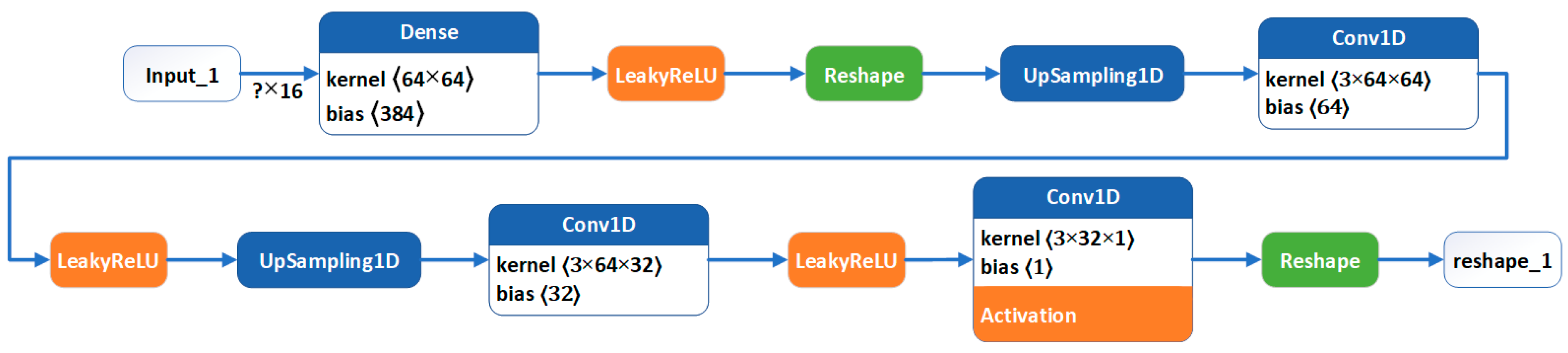
2.6.1. Generator
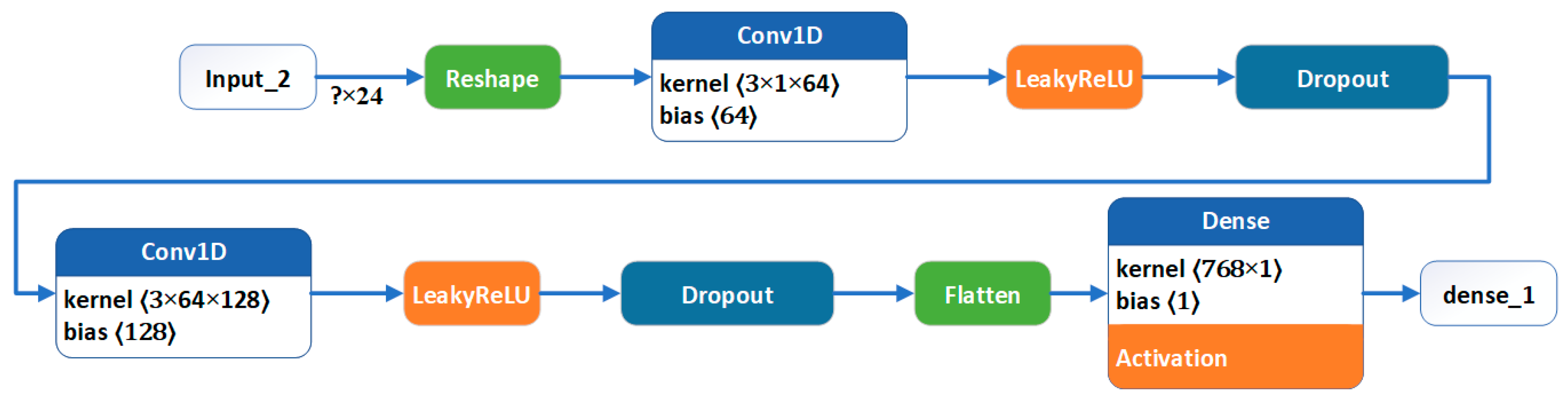
2.6.2. Discriminator
| Algorithm 1. Conv1D-WGAN-GP |
| 1: Input: A Dataset of load profiles 2: Output: A synthetic dataset of load profiles 3: Initiate Critic variables: number of critics 4: Build the Generator: 5: Build the Discriminator (Critic): 6: Define the Gradient Penalty function: 7: Train model 8: Train model 9: Train Conv1D-WGAN-GP: 10: for each epoch do: 11: for each number of critics do: 12: Sample random noise vector 13: Sample a batch of real samples x from the training data 14: Generate fake samples 15: Compute the critic loss 16: Update critic D using gradients of 17: end for 18: Sample random noise vector 19: Generate fake samples 20: Compute generator loss— 21: Update generator using gradients of 22: end for 23: Generate Synthetic Data: 24: Sample noise vectors 25: Generate synthetic samples: |
2.6.3. Hyperparameters
- Latent Dimension: 8, 16, 32;
- Batch Size: 32, 64, 128;
- Epochs: Fixed at 1000 for comparability;
- Number of Critics: 3, 5, 10;
- Gradient Penalty Coefficient λ: 1, 2, 5, 10.
3. Results
3.1. Experimental Datasets
3.1.1. Publicly Available Residential Dataset
3.1.2. Industrial Dataset
3.1.3. Household
3.1.4. Pig Farm
3.1.5. Data Preprocessing
- Normalization—all datasets are min–max normalized independently to scale hourly consumption values into the [0, 1] range. This normalization is performed per dataset to avoid leakage of information across domains and to ensure that the generator outputs remain within valid ranges for each specific case;
- Missing Value Handling—for the Household dataset, which contained intermittent missing values due to sensor outages or gaps in measurement, linear interpolation was applied within each 24 h profile to fill missing hourly entries (when gaps were ≤2 h). Days with more than two missing hours were excluded from the dataset;
- Profile Validation—only days with complete 24 h load profiles (after preprocessing) are retained. This ensures uniform input dimensionality for the GAN training.
3.2. Evaluation and Comparison
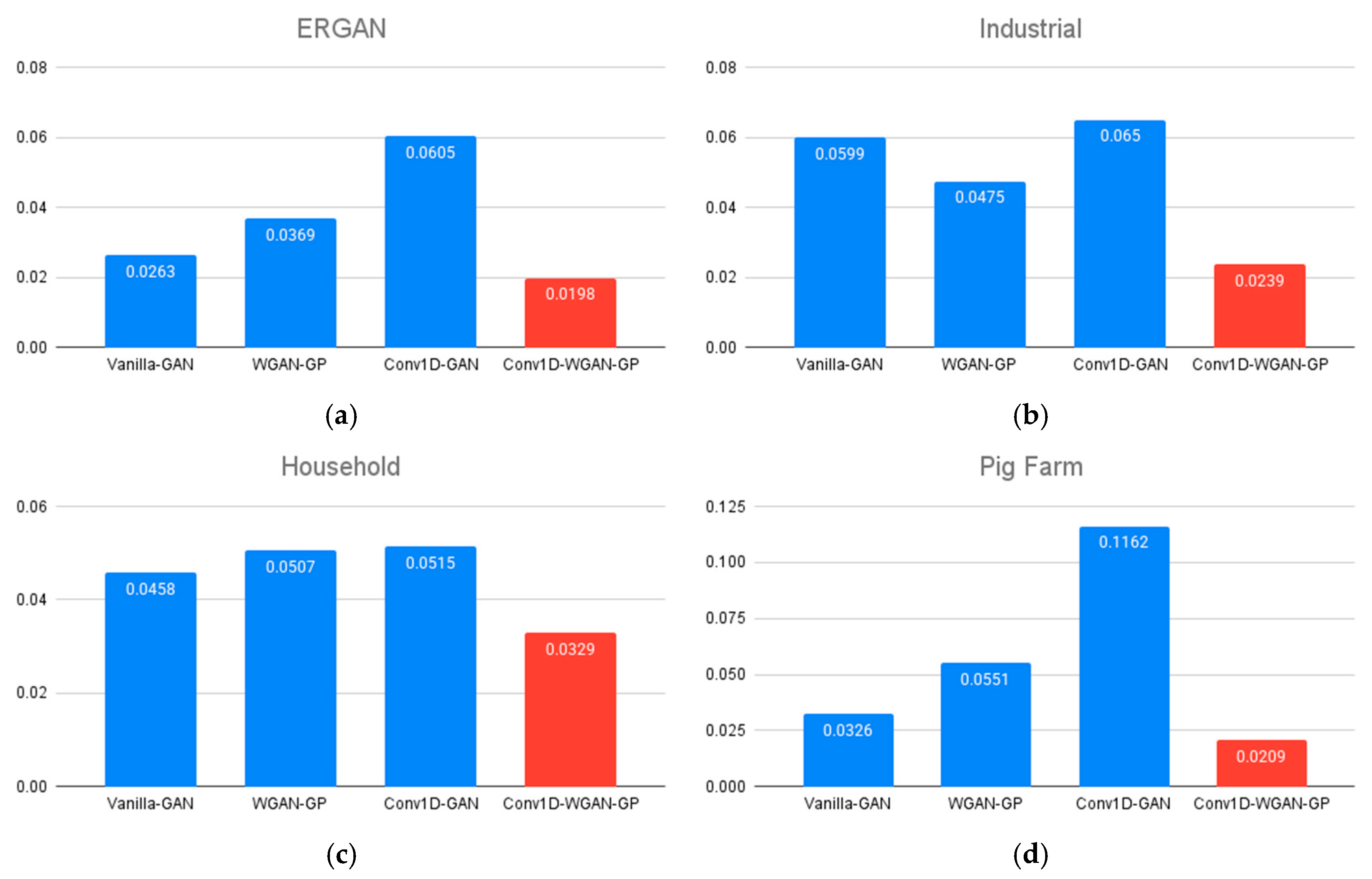
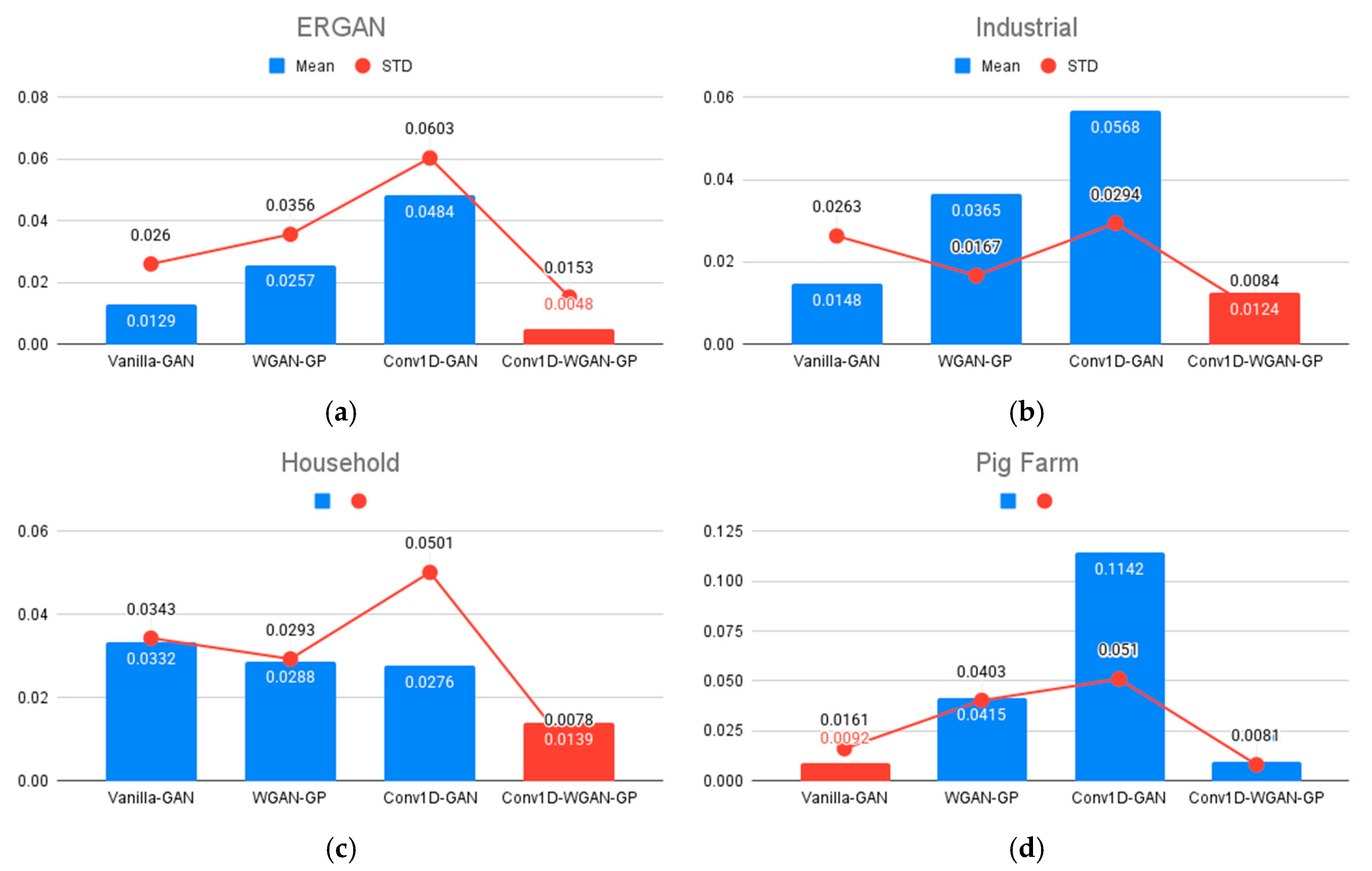
3.2.1. Statistical Methods for Evaluation of the Synthetic Data
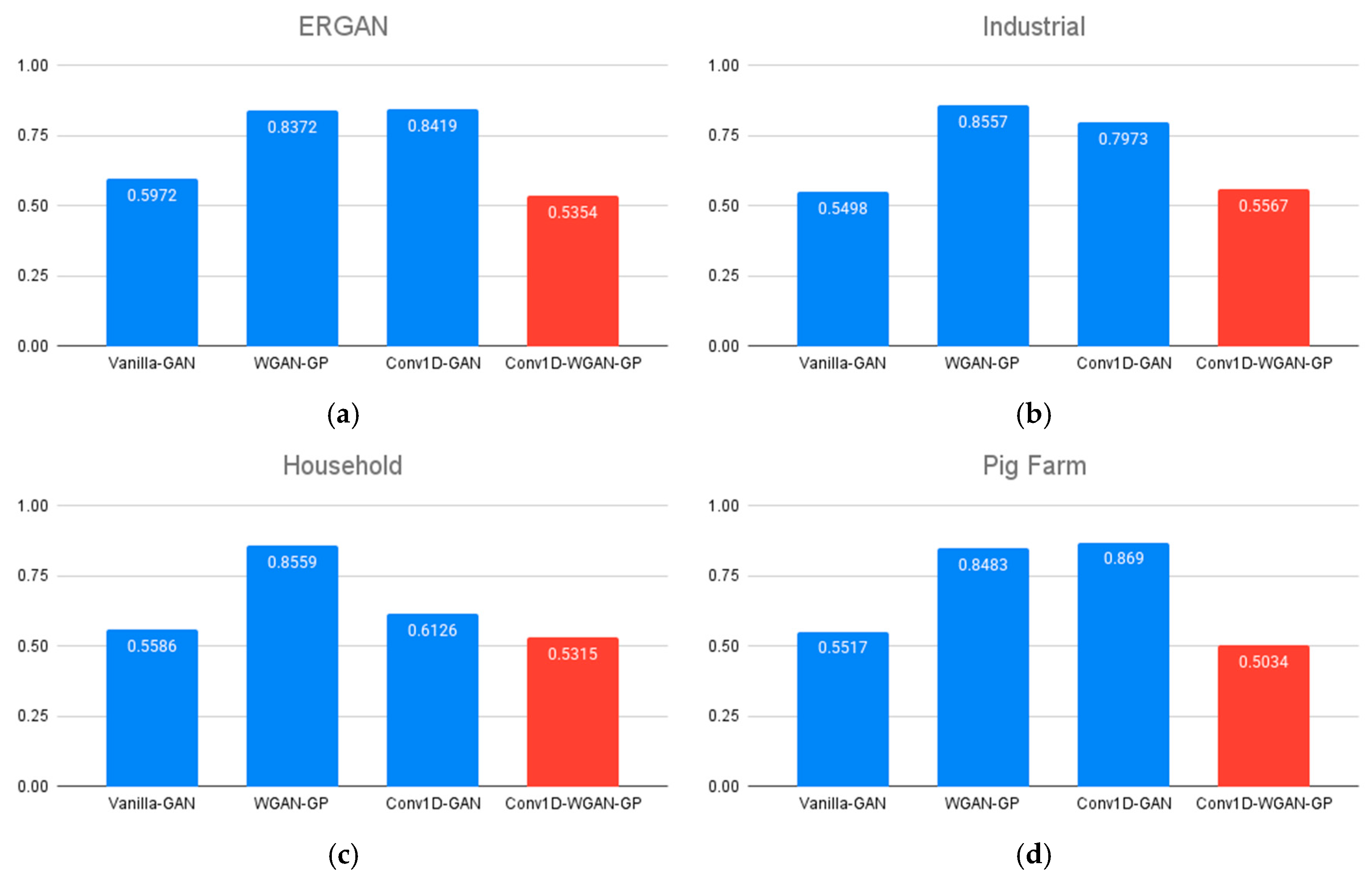
3.2.2. Downstream Tasks for Evaluation of the Synthetic Data
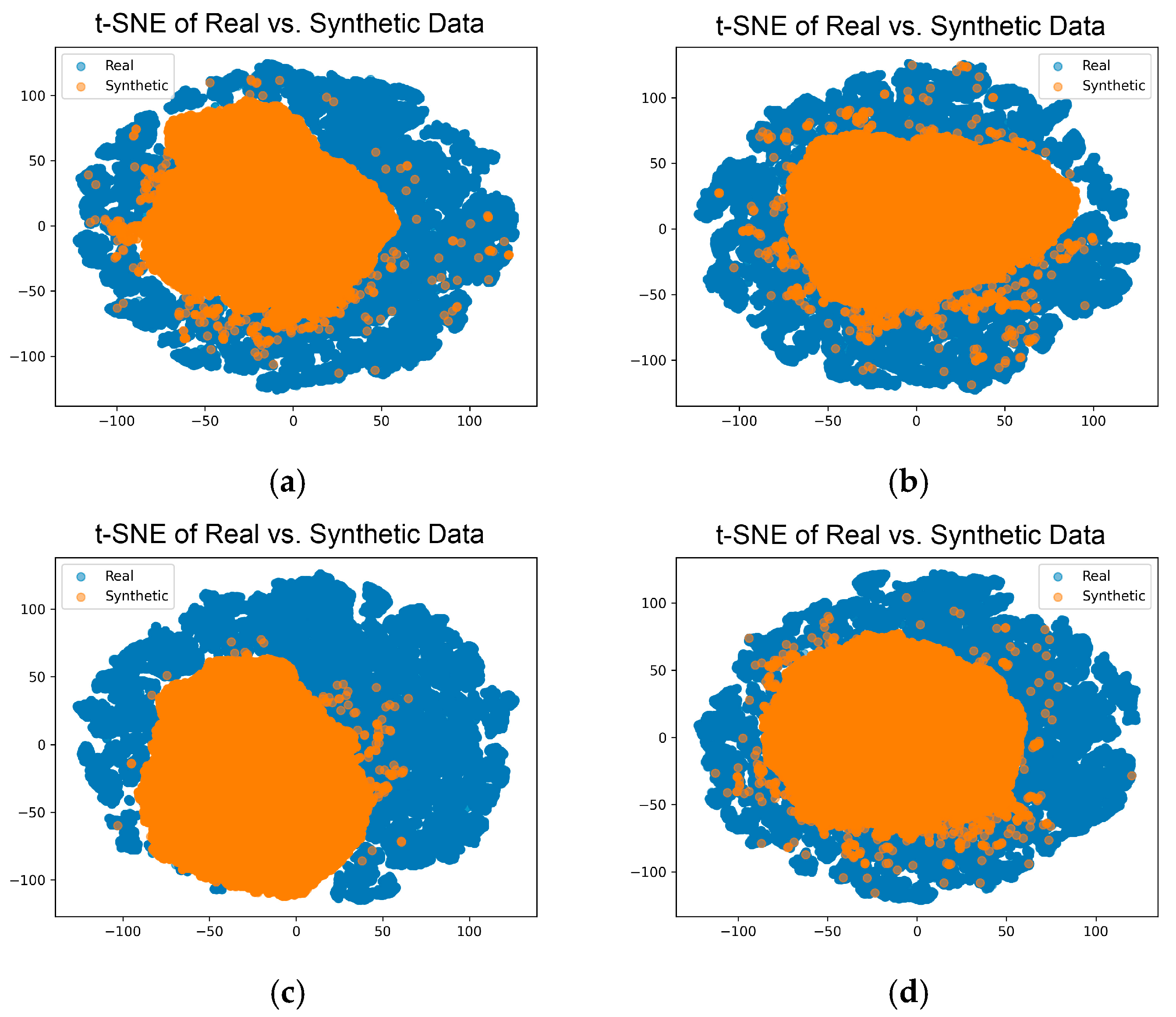
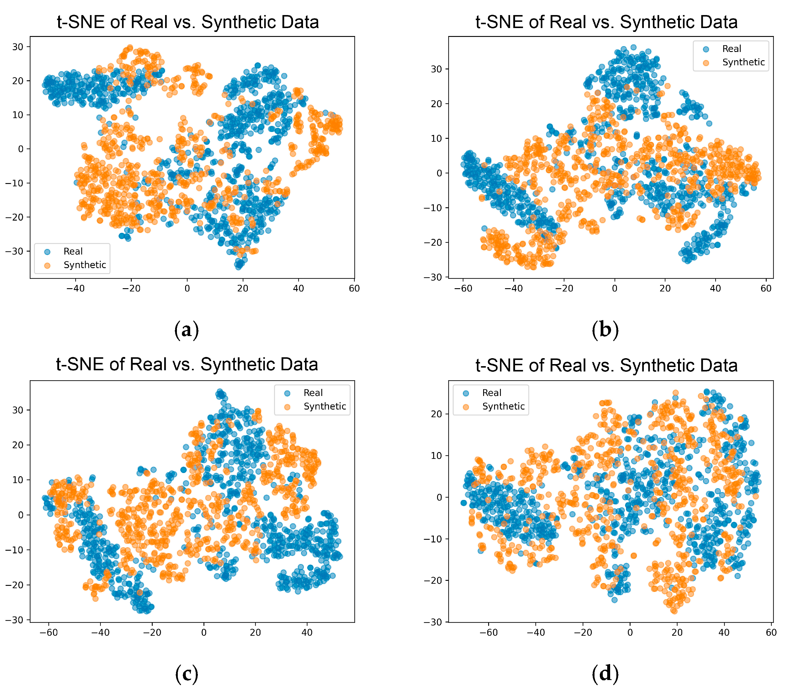
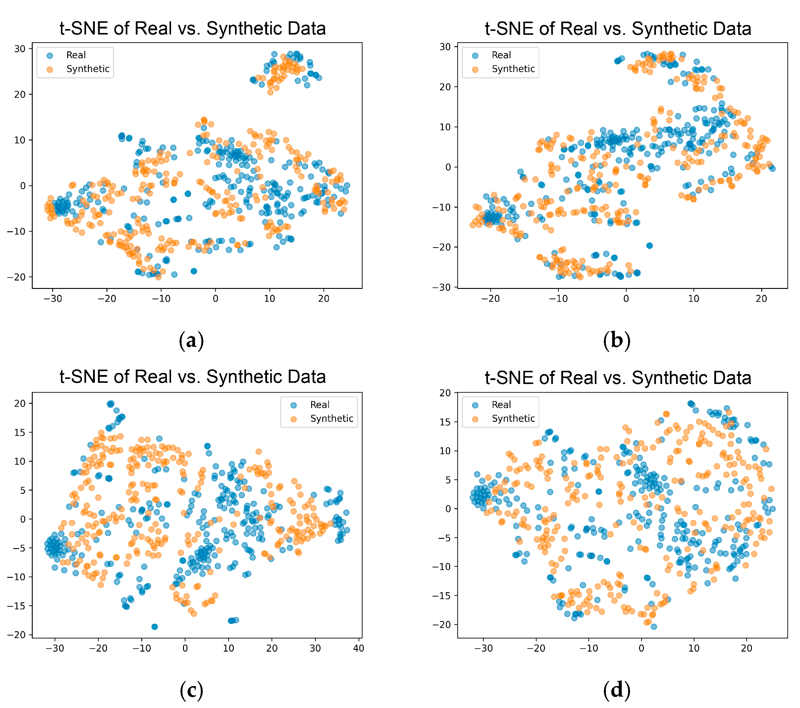
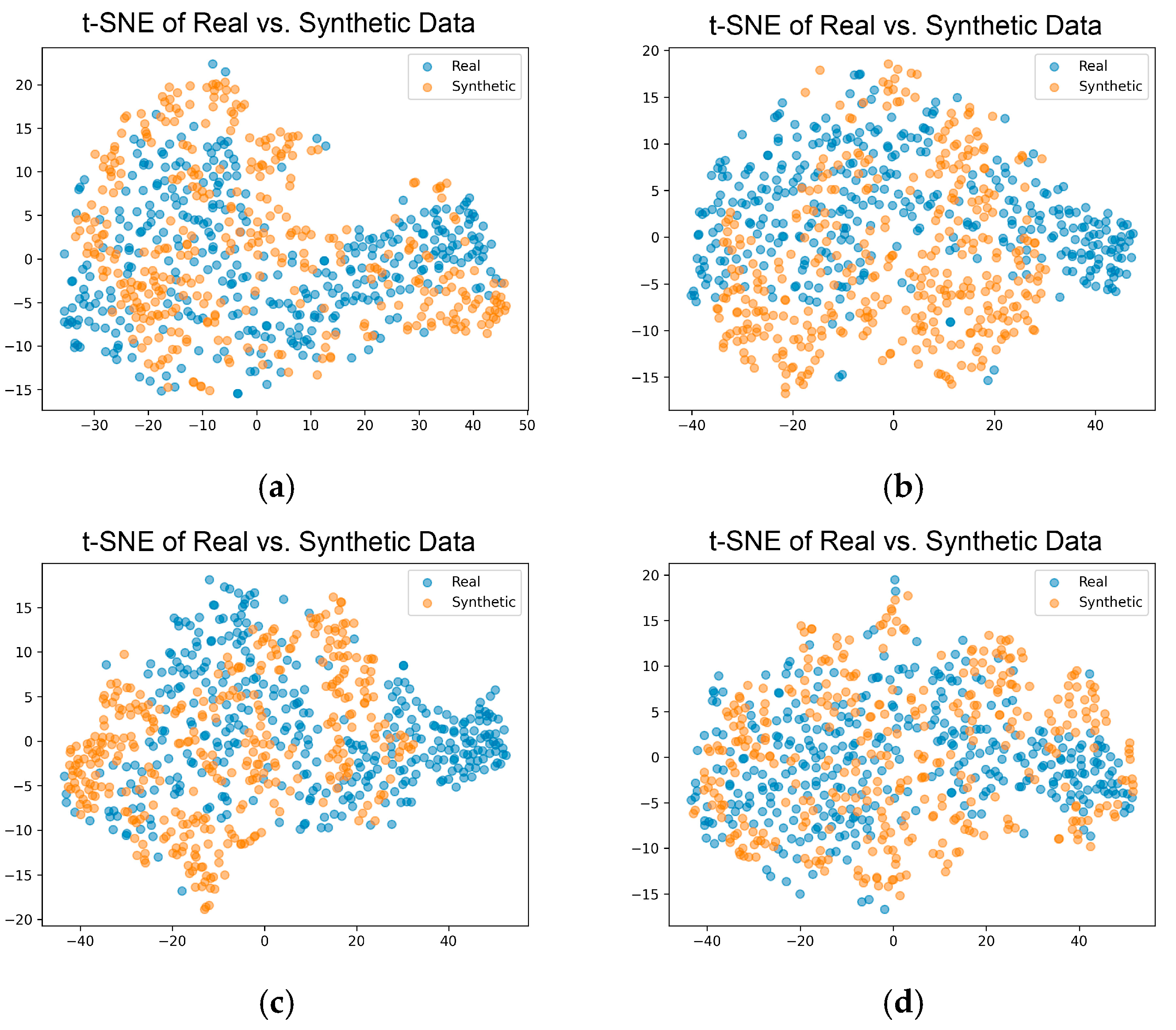
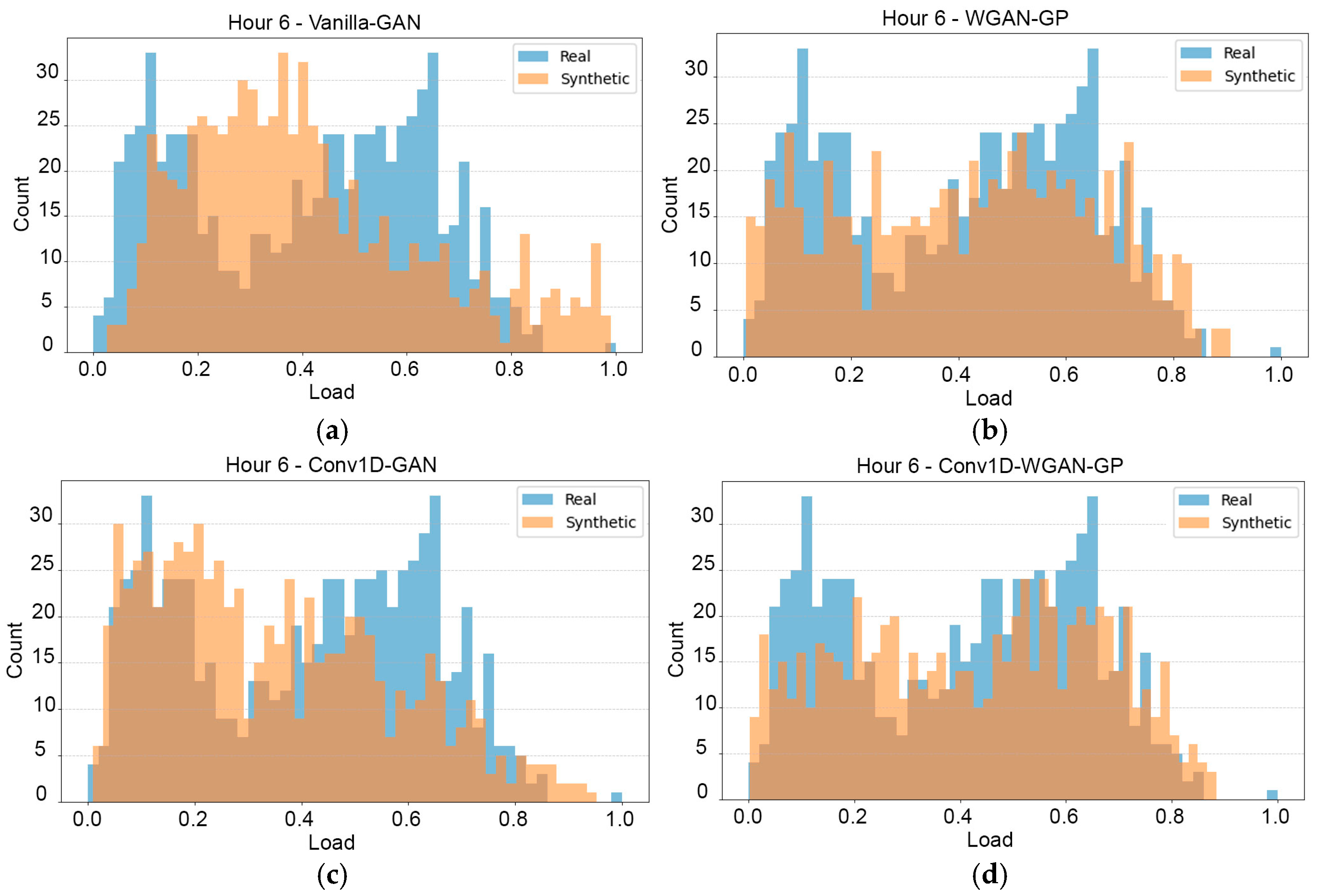
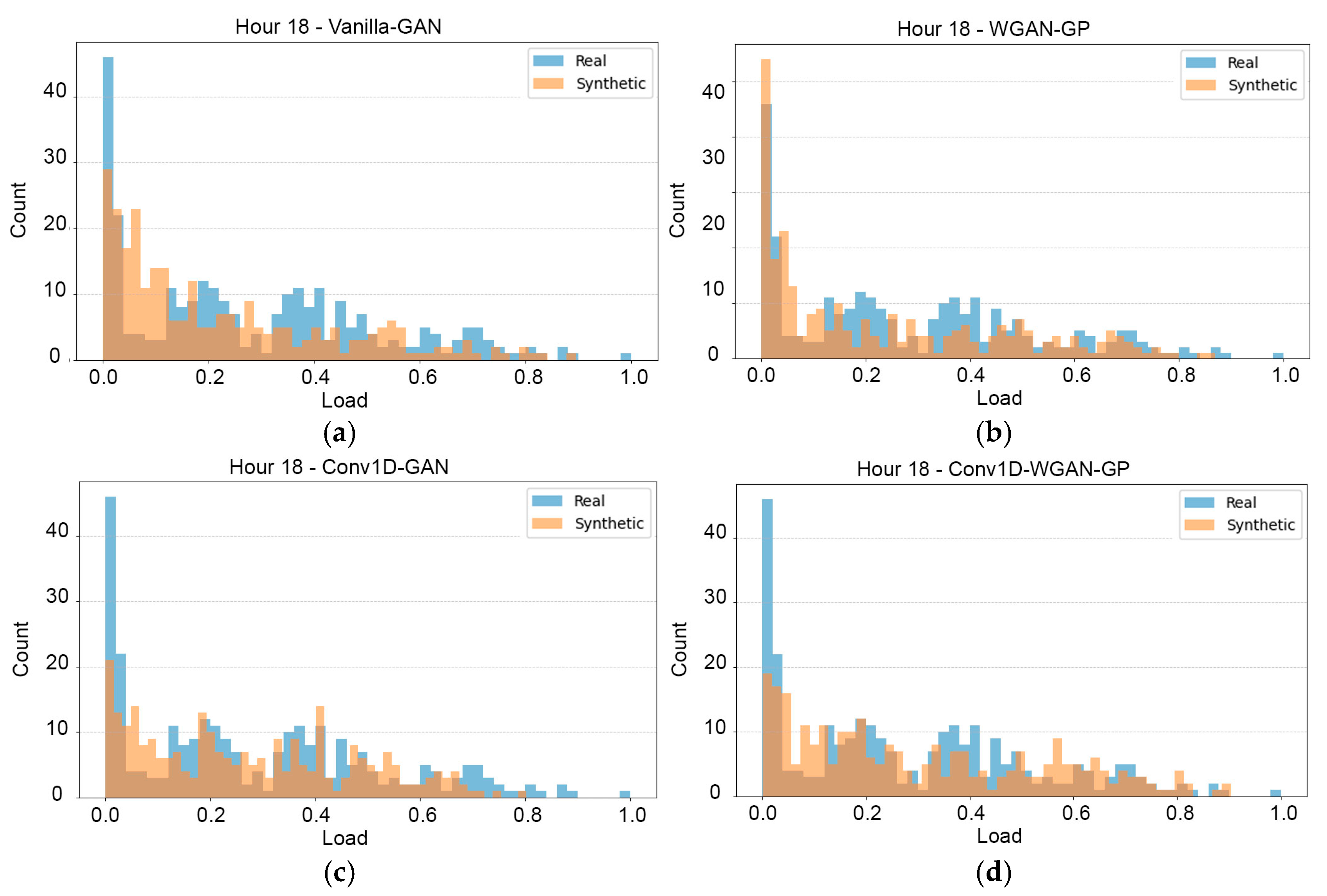
3.2.3. Visual Methods for Evaluation of the Synthetic Data
3.2.4. Overall Model Performance of Conv1D-WGAN-GP
4. Discussion
4.1. Dataset Size Sensitivity
4.2. Role of GANs in Load Profile Generation
4.3. Proposed Conv1D-WGAN-GP Model
4.4. Limitations
5. Conclusions
Author Contributions
Funding
Institutional Review Board Statement
Informed Consent Statement
Data Availability Statement
Conflicts of Interest
References
- Wang, Z.; Hong, T. Generating realistic building electrical load profiles through the Generative Adversarial Network (GAN). Energy Build. 2020, 224, 110299. [Google Scholar] [CrossRef]
- Price, P. Methods for Analyzing Electric Load Shape and Its Variability; Lawrence Berkeley National Laboratory: Berkeley, CA, USA, 2010. Available online: https://www.osti.gov/biblio/985909 (accessed on 15 May 2025).
- Valova, I.; Gabrovska-Evstatieva, K.G.; Kaneva, T.; Evstatiev, B.I. Generation of Realistic Synthetic Load Profile Based on the Markov Chains Theory: Methodology and Case Studies. Algorithms 2025, 18, 287. [Google Scholar] [CrossRef]
- Conselvan, F.; Mascherbauer, P.; Harringer, D. Neural network to generate synthetic building electrical load profiles. In Proceedings of the 13 Internationale Energiewirtschaftstagung an der TU Wien (IEWT), Vien, Austria, 15–17 February 2023. [Google Scholar]
- Hu, J.; Vasilakos, A.V. Energy big data analytics and security: Challenges and opportunities. IEEE Trans. Smart Grid 2016, 7, 2423–2436. [Google Scholar] [CrossRef]
- Triastcyn, A.; Faltings, B. Generating Higher-Fidelity Synthetic Datasets with Privacy Guarantees. Algorithms 2022, 15, 232. [Google Scholar] [CrossRef]
- Wang, C.; Tindemans, S.H.; Palensky, P. Generating contextual load profiles using a conditional variational autoencoder. In Proceedings of the 2022 IEEE PES Innovative Smart Grid Technologies Conference Europe (ISGT-Europe), Novi Sad, Serbia, 10–12 October 2022; IEEE: New York, NY, USA, 2022; pp. 1–6. [Google Scholar] [CrossRef]
- Molina-Markham, A.; Shenoy, P.; Fu, K.; Cecchet, E.; Irwin, D. Private memoirs of a smart meter. In Proceedings of the 2nd ACM Workshop on Embedded Sensing Systems for Energy-Efficiency in Building, Zurich, Switzerland, 2 November 2010; pp. 61–66. [Google Scholar] [CrossRef]
- Wang, W.; Hong, T.; Li, N.; Wang, R.Q.; Chen, J. Linking energy-cyber-physical systems with occupancy prediction and interpretation through WiFi probe-based ensemble classification. Appl. Energy 2019, 236, 55–69. [Google Scholar] [CrossRef]
- Wang, Z.; Hong, T.; Piette, M.A. Data fusion in predicting internal heat gains for office buildings through a deep learning approach. Appl. Energy 2019, 240, 386–398. [Google Scholar] [CrossRef]
- Hassija, V.; Chamola, V.; Mahapatra, A.; Singal, A.; Goel, D.; Huang, K.; Scardapane, S.; Spinelli, I.; Mahmud, M.; Hussain, A. Interpreting black-box models: A review on explainable artificial intelligence. Cogn. Comput. 2024, 16, 45–74. [Google Scholar] [CrossRef]
- Lin, Z.; Jain, A.; Wang, C.; Fanti, G.; Sekar, V. Using GANs for Sharing Networked Time Series Data: Challenges, Initial Promise, and Open Questions. In Proceedings of the IMC ‘20: Proceedings of the ACM Internet Measurement Conference, Virtual Event, 27 October 2020; Association for Computing Machinery: New York, NY, USA, 2020; pp. 464–483. [Google Scholar] [CrossRef]
- Labeeuw, W.; Deconinck, G. Residential Electrical Load Model Based on Mixture Model Clustering and Markov Models. IEEE Trans. Ind. Inform. 2013, 9, 1561–1569. [Google Scholar] [CrossRef]
- Blanco, L.; Zabala, A.; Schiricke, B.; Hoffschmidt, B. Generation of heat and electricity load profiles with high temporal resolution for Urban Energy Units using open geodata. Sustain. Cities Soc. 2024, 117, 105967. [Google Scholar] [CrossRef]
- Munkhammar, J.; van der Meer, D.; Widén, J. Very short term load forecasting of residential electricity consumption using the Markov-chain mixture distribution (MCM) model. Appl. Energy 2021, 282, 116180. [Google Scholar] [CrossRef]
- Dalla Maria, E.; Secchi, M.; Macii, D. A Flexible Top-Down Data-Driven Stochastic Model for Synthetic Load Profiles Generation. Energies 2022, 15, 269. [Google Scholar] [CrossRef]
- McLoughlin, F.; Duffy, A.; Conlon, M. The generation of domestic electricity load profiles through Markov chain modelling. In Proceedings of the 3rd International Scientific Conference on Energy and Climate Change Conference, Athens, Greece, 7–8 October 2010; pp. 18–27. Available online: https://arrow.tudublin.ie/dubencon2/9/ (accessed on 12 April 2025).
- Tushar, W.; Huang, S.; Yuen, C.; Zhang, J.A.; Smith, D.B. Synthetic generation of solar states for smart grid: A multiple segment Markov chain approach. In Proceedings of the IEEE PES Innovative Smart Grid Technologies, Europe, Istanbul, Turkey, 12–15 October 2014; IEEE: New York, NY, USA, 2014; pp. 1–6. [Google Scholar] [CrossRef]
- Pillai, G.G.; Putrus, G.A.; Pearsall, N.M. Generation of synthetic benchmark electrical load profiles using publicly available load and weather data. Int. J. Electr. Power Energy Syst. 2014, 61, 1–10. [Google Scholar] [CrossRef]
- Tamayo-Urgilés, D.; Sanchez-Gordon, S.; Valdivieso Caraguay, Á.L.; Hernández-Álvarez, M. GAN-Based Generation of Synthetic Data for Vehicle Driving Events. Appl. Sci. 2024, 14, 9269. [Google Scholar] [CrossRef]
- Bhattarai, B.; Baek, S.; Bodur, R.; Kim, T.K. Sampling strategies for gan synthetic data. In Proceedings of the ICASSP 2020–2020 IEEE International Conference on Acoustics, Speech and Signal Processing (ICASSP), Barcelona, Spain, 4–8 May 2020; IEEE: New York, NY, USA, 2020. [Google Scholar] [CrossRef]
- Pan, Z.; Wang, J.; Liao, W.; Chen, H.; Yuan, D.; Zhu, W.; Fang, X.; Zhu, Z. Data-Driven EV Load Profiles Generation Using a Variational Auto-Encoder. Energies 2019, 12, 849. [Google Scholar] [CrossRef]
- Goodfellow, I.J.; Pouget-Abadie, J.; Mirza, M.; Xu, B.; Warde-Farley, D.; Ozair, S.; Courville, A.; Bengio, Y. Generative adversarial networks. Commun. ACM 2020, 63, 139–144. [Google Scholar] [CrossRef]
- Gu, Y.; Chen, Q.; Liu, K.; Xie, L.; Kang, C. GAN-based model for residential load generation considering typical consumption patterns. In Proceedings of the 2019 IEEE Power & Energy Society Innovative Smart Grid Technologies Conference (ISGT), Washington, DC, USA, 18–21 February 2019; pp. 1–5. [Google Scholar] [CrossRef]
- Liang, X.; Wang, Z.; Wang, H. Synthetic Data Generation for Residential Load Patterns via Recurrent GAN and Ensemble Method. IEEE Trans. Instrum. Meas. 2024, 73, 2535412. [Google Scholar] [CrossRef]
- Jordon, J.; Yoon, J.; Van Der Schaar, M. PATE-GAN: Generating synthetic data with differential privacy guarantees. In Proceedings of the International Conference on Learning Representations, Vancouver, BC, Canada, 21 December 2018. [Google Scholar]
- Xu, L.; Skoularidou, M.; Cuesta-Infante, A.; Veeramachaneni, K. Modeling tabular data using conditional GAN. In Proceedings of the 33rd Conference on Neural Information Processing Systems (NeurIPS 2019), Vancouver, BC, Canada, 8–14 December 2019. [Google Scholar]
- Walia, M.S.; Tierney, B.; McKeever, S. Synthesising tabular datasets using Wasserstein Conditional GANS with Gradient Penalty (WCGAN-GP). In Proceedings of the AICS 2020: 28th Irish Conference on Artificial Intelligence and Cognitive Science, Dublin, Ireland, 7–8 December 2020. [Google Scholar]
- Gulrajani, I.; Ahmed, F.; Arjovsky, M.; Dumoulin, V.; Courville, A.C. Improved training of Wasserstein GANs. In Proceedings of the 31st International Conference on Neural Information Processing Systems, NIPS’17, Long Beach, CA, USA, 31 March 2017; Curran Associates Inc.: Red Hook, NY, USA, 2017; pp. 5769–5779. [Google Scholar]
- Ha, T.; Dang, T.K.; Dang, T.T.; Truong, T.A.; Nguyen, M.T. Differential privacy in deep learning: An overview. In Proceedings of the 2019 International Conference on Advanced Computing and Applications (ACOMP), Nha Trang, Vietnam, 26–28 November 2019; pp. 97–102. [Google Scholar] [CrossRef]
- Impraimakis, M. A Kullback–Leibler divergence method for input–system–state identification. J. Sound Vib. 2024, 569, 117965. [Google Scholar] [CrossRef]
- Johnson, D.H.; Sinanovic, S. Symmetrizing the Kullback-Leibler distance. IEEE Trans. Inf. Theory 2001, 1, 1–10. [Google Scholar]
- Menéndez, M.L.; Pardo, J.A.; Pardo, L.; Pardo, M.C. The Jensen-Shannon divergence. J. Frankl. Inst. 1997, 334, 307–318. [Google Scholar] [CrossRef]
- Sinn, M.; Rawat, A. Non-parametric estimation of Jensen-Shannon divergence in generative adversarial network training. In Proceedings of the International Conference on Artificial Intelligence and Statistics, Playa Blanca, Lanzarote, Canary Islands, Spain, 9–11 April 2018; pp. 642–651. [Google Scholar]
- Yoon, J.; Jarrett, D.; der Schaar, M. Time-series generative adversarial networks. In Proceedings of the 33rd International Conference on Neural Information Processing Systems, Vancouver, BC, Canada, 8–14 December 2019; Volume 494, pp. 5508–5518. [Google Scholar]
- Aloni, O.; Perelman, G.; Fishbain, B. Synthetic random environmental time series generation with similarity control, preserving original signal’s statistical characteristics. Environ. Model. Softw. 2025, 185, 106283. [Google Scholar] [CrossRef]
- Milne, T.; Nachman, A.I. Wasserstein GANs with gradient penalty compute congested transport. Conf. Learn. Theory 2022, 178, 103–129. [Google Scholar]
- Lee, G.-C.; Li, J.-H.; Li, Z.-Y. A Wasserstein generative adversarial network-gradient penalty-based model with imbalanced data enhancement for network intrusion detection. Appl. Sci. 2023, 13, 8132. [Google Scholar] [CrossRef]
- Arjovsky, M.; Chintala, S.; Bottou, L. Wasserstein generative adversarial networks. In Proceedings of the 34th International Conference on Machine Learning, Sydney, Australia, 6–11 August 2017; pp. 214–223. [Google Scholar]
- Weng, L. From GAN to WGAN. arXiv 2019, arXiv:1904.08994. [Google Scholar]
- ERGAN-Dataset. Available online: https://github.com/AdamLiang42/ERGAN-Dataset (accessed on 1 May 2025).
- Pecan Street Database. Available online: https://www.pecanstreet.org/work/energy/ (accessed on 1 May 2025).


| Metric | Threshold Values * | The Metric’s Importance in This Methodology |
|---|---|---|
| Average Wasserstein Distance [35] | <0.15 (Excellent), <0.25 (Good) | Measures distribution alignment per hour. Lower is better; high values indicate poor matching of load shapes. |
| Mean Difference [36] | <0.05 (Excellent), <0.10 (Acceptable) | Ensures the synthetic data have the same overall average load. |
| STD Difference [36] | <0.1 (Excellent), <0.2 (Acceptable) | Captures variability; essential for representing diversity in users’ behavior. |
| Classifier Accuracy (logistic regression) | ≤0.6 (Ideal), ≤0.65 (Tolerable) | If a simple model cannot easily distinguish real from synthetic, it indicates high realism. |
| JS Divergence (overall) | <0.05 (Excellent), <0.1 (Good) | A symmetric version of KL. Easier to interpret; 0 = identical, 1 = total difference. |
| RMSE (per profile and overall) | <0.1 (Excellent), <0.2 (Acceptable) | Penalizes large point-wise errors. It should be small if the curves are aligned. |
| Model | Characteristic | Value |
|---|---|---|
| Generator | 1st layer: | Densely connected: 128 units; activation—LeakyReLU |
| 2nd layer: | Batch normalization | |
| 3rd layer: | Densely connected: 256 units; activation—LeakyReLU | |
| 4th layer: | Batch normalization | |
| Output: | Densely connected: 24 units; activation—sigmoid | |
| Loss function: | Binary cross-entropy | |
| Optimizer | Adam (Adaptive moment estimation): learning rate = 0.0002; | |
| Discriminator | 1st layer: | Densely connected: 256 units; activation—LeakyReLU |
| 2nd layer: | Dropout: dropout rate = 0.3 | |
| 3rd layer: | Densely connected: 128 units; activation—LeakyReLU | |
| 4th layer: | Dropout: dropout rate = 0.3 | |
| Output: | Densely connected: 1 unit; activation—sigmoid | |
| Loss function: | Binary cross-entropy | |
| Optimizer | Adam (adaptive moment estimation): learning rate = 0.0002 |
| Model | Characteristic | Value |
|---|---|---|
| Generator | 1st layer: | Densely connected: 128 units; activation—LeakyReLU |
| 2nd layer: | batch normalization | |
| 3rd layer: | Densely connected: 256 units; activation—LeakyReLU | |
| 4th layer: | batch normalization | |
| 5th layer: | Densely connected: 128 units; activation—LeakyReLU | |
| Output: | Densely connected: 24 units; activation—sigmoid | |
| Loss function: | Wasserstein loss | |
| Optimizer | Adam (adaptive moment estimation): learning rate = 0.0002; | |
| Discriminator | 1st layer: | Densely connected: 128 units; activation—LeakyReLU |
| 2nd layer: | dropout; dropout rate = 0.3 | |
| 3rd layer: | Densely connected: 64 units; activation—LeakyReLU | |
| 4th layer: | dropout; dropout rate = 0.3 | |
| Output: | Densely connected: 1 unit; activation—none | |
| Loss function: | Wasserstein loss | |
| Optimizer | Adam (adaptive moment estimation): learning rate = 0.0002; |
| Model | Characteristic | Values |
|---|---|---|
| Generator | 1st layer: | Densely connected: 384 units; activation—LeakyReLU |
| 2nd layer: | Reshape: (6, 64) | |
| 3rd layer: | UpSampling1D: size = 2 → (12, 64) | |
| 4th layer: | Convolutional: 64 filters, kernel size = 3, padding = ‘same’; activation—LeakyReLU | |
| 5th layer: | UpSampling1D: size = 2 → (24, 64) | |
| 6th layer: | Convolutional: 32 filters, kernel size = 3, padding = ‘same’; activation—LeakyReLU | |
| Output: | Convolutional: 1 filter, kernel size = 3, activation = sigmoid, padding = “same”; followed by reshape to (24,) | |
| Loss function: | Binary cross-entropy | |
| Optimizer | Adam (adaptive moment estimation): learning rate = 0.0002 | |
| Discriminator | 1st layer: | Input: shape (24,) |
| 2nd layer: | Reshape: (24, 1) | |
| 3rd layer: | Convolutional: 64 filters, kernel size = 3, strides = 2, padding = “same”; activation—LeakyReLU | |
| 4th layer: | Dropout: rate = 0.3 | |
| 5th layer: | Convolutional: 128 filters, kernel size = 3, strides = 2, padding = “same”; activation—LeakyReLU | |
| 6th layer: | Dropout: rate = 0.3 | |
| 7th layer: | Flatten | |
| Output: | Densely connected: 1 unit; activation—sigmoid | |
| Loss function: | Binary cross-entropy | |
| Optimizer | Adam (adaptive moment estimation): learning rate = 0.0002 |
| Hyperparameter | Value |
|---|---|
| Latent Dimension | 16 |
| Batch Size | 128 |
| Epochs | 1000 |
| Number of Critics | 10 |
| Lambda | 2 |
| Dataset | Number of Samples | Duration |
|---|---|---|
| ERGAN-dataset | 110,274 | N/A 1 |
| Industrial | 728 | 2 years |
| Household | 278 | 1 year |
| Pig Farm | 363 | 1 year |
| Dataset | Model | W-Distance | Mean Diff. | STD Diff. 1 | Classifier Acc. 2 | JS Div. 3 | RMSE 4 |
|---|---|---|---|---|---|---|---|
| ERGAN | Vanilla-GAN | 0.0263 | 0.0129 | 0.026 | 0.5972 | 0.0023 | 0.2669 |
| WGAN-GP | 0.0369 | 0.0257 | 0.0356 | 0.8372 | 0.0091 | 0.2709 | |
| Conv1D-GAN | 0.0605 | 0.0484 | 0.0603 | 0.8419 | 0.0193 | 0.2633 | |
| Conv1D-WGAN-GP | 0.0198 | 0.0048 | 0.0153 | 0.5354 | 0.0176 | 0.2647 | |
| Industrial | Vanilla-GAN | 0.0599 | 0.0148 | 0.0263 | 0.5498 | 0.0329 | 0.2864 |
| WGAN-GP | 0.0475 | 0.0365 | 0.0167 | 0.8557 | 0.0087 | 0.2893 | |
| Conv1D-GAN | 0.065 | 0.0568 | 0.0294 | 0.7973 | 0.017 | 0.2763 | |
| Conv1D-WGAN-GP | 0.0239 | 0.0124 | 0.0084 | 0.5567 | 0.0062 | 0.2716 | |
| Household | Vanilla-GAN | 0.0458 | 0.0332 | 0.0343 | 0.5586 | 0.0309 | 0.3109 |
| WGAN-GP | 0.0507 | 0.0288 | 0.0293 | 0.8559 | 0.0348 | 0.3317 | |
| Conv1D-GAN | 0.0515 | 0.0276 | 0.0501 | 0.6126 | 0.0494 | 0.2871 | |
| Conv1D-WGAN-GP | 0.0329 | 0.0139 | 0.0078 | 0.5315 | 0.0341 | 0.3219 | |
| Pig Farm | Vanilla-GAN | 0.0326 | 0.0092 | 0.0161 | 0.5517 | 0.0162 | 0.2833 |
| WGAN-GP | 0.0551 | 0.0415 | 0.0403 | 0.8483 | 0.0138 | 0.2549 | |
| Conv1D-GAN | 0.1162 | 0.1142 | 0.051 | 0.869 | 0.0565 | 0.277 | |
| Conv1D-WGAN-GP | 0.0209 | 0.0096 | 0.0081 | 0.5034 | 0.0078 | 0.2801 |
Disclaimer/Publisher’s Note: The statements, opinions and data contained in all publications are solely those of the individual author(s) and contributor(s) and not of MDPI and/or the editor(s). MDPI and/or the editor(s) disclaim responsibility for any injury to people or property resulting from any ideas, methods, instructions or products referred to in the content. |
© 2025 by the authors. Licensee MDPI, Basel, Switzerland. This article is an open access article distributed under the terms and conditions of the Creative Commons Attribution (CC BY) license (https://creativecommons.org/licenses/by/4.0/).
Share and Cite
Kaneva, T.; Valova, I.; Gabrovska-Evstatieva, K.; Evstatiev, B. A Data-Driven Approach for Generating Synthetic Load Profiles with GANs. Appl. Sci. 2025, 15, 7835. https://doi.org/10.3390/app15147835
Kaneva T, Valova I, Gabrovska-Evstatieva K, Evstatiev B. A Data-Driven Approach for Generating Synthetic Load Profiles with GANs. Applied Sciences. 2025; 15(14):7835. https://doi.org/10.3390/app15147835
Chicago/Turabian StyleKaneva, Tsvetelina, Irena Valova, Katerina Gabrovska-Evstatieva, and Boris Evstatiev. 2025. "A Data-Driven Approach for Generating Synthetic Load Profiles with GANs" Applied Sciences 15, no. 14: 7835. https://doi.org/10.3390/app15147835
APA StyleKaneva, T., Valova, I., Gabrovska-Evstatieva, K., & Evstatiev, B. (2025). A Data-Driven Approach for Generating Synthetic Load Profiles with GANs. Applied Sciences, 15(14), 7835. https://doi.org/10.3390/app15147835