Design of a Methodology to Evaluate the Energy Flexibility of Residential Consumers to Enhance Household Demand Side Management: The Case of a Spanish Municipal Network

Abstract

Climate change and global warming are causing growing environmental concerns, prompting many countries to increase investments in renewable energies. The high growth rate of renewables in the energy systems brings significant intermittency challenges. Demand-side flexibility is presented as a viable solution to address this phenomenon. In this framework, this research study proposes a novel methodology to evaluate the flexibility potential that residential consumers can offer to the Distribution System Operator (DSO). Moreover, it pretends to provide guidelines and design of standardized parameters to disaggregate the aggregated energy consumption data of end-users. This step is essential to identify and characterize the primary energy consumption processes in the residential sector, laying the groundwork for future flexibility evaluation. Furthermore, the modeling of the energy consumption curves will enhance residential sector demand-side flexibility enabling end-users to modify their usual consumption patterns. The implemented methodology has been applied to real consumer data provided by the DSO of a Spanish municipality of about 29,000 habitants in the Alicante Province (Spain). Results achieved allowed the validation of the proposed methodology enabling the disaggregation of residential energy profiles and facilitating the subsequent dynamic assessment of residential end-user’s demand flexibility. Moreover, this work will provide valuable guidelines to carry out short-term energy resource planning and solve operational problems of the energy systems.

1. Introduction

Climate change and greenhouse gas emissions are currently a primary global concern. The European Union has set out an ambitious plan to combat global warming, aiming for a 45% reduction in greenhouse gas emissions by 2030 and the complete climate neutrality by 2050 [1]. One of the main approaches to achieve this goal is decarbonizing energy systems by integrating renewable energy sources, such as solar and wind, into the energy mix [2].

This energy trend significantly increases the intermittency of electricity supply due to the variable nature of these sources [3]. Fluctuation in renewable energy production can lead to supply gaps when demand exceeds production capacity, or on cloudy or windless days, necessitating a more flexible and resilient energy system to maintain grid stability. Demand response mechanisms have been implemented to mitigate this challenge, taking advantage of the flexibility of energy consumption [4].

Demand flexibility allows consumers, belonging from different sectors, residential [5], commercial [6], and industrial [7], to adapt their consumption to the electricity system’s needs, either in the case of energy shortages or in situations of risk to grid reliability due to unexpected failures [3,8]. The industrial sector is one of the main consumers of electricity. Consequently, demand-side flexibility holds a unique potential for its stability and flexibility that can be implemented directly by modifying factories’ operating hours [9]. Instead, in the residential sector, demand-side management does not still have a clear application due to the uncertainty of the end user consumption patterns and the lack of regulations and smart energy infrastructure [10]. Furthermore, the analysis of flexibility in a factory differs substantially from that of a household, where home energy management systems (HEMS) can provide more granular control over appliance consumption but must be easily integrated into daily life without disrupting daily activities [11]. Residential flexibility is mainly achieved through connected devices and task automation. It allows households to decrease their consumption at times of high demand or taking advantage of periods of lower energy cost for activities such as charging electric vehicles or scheduling heating and cooling. In the residential sector, HEMS act as innovative platforms to optimize the consumption of household appliances such as washing machines [12], electric water heaters [13], ovens [14], dryers [15], dishwashers [16], lighting systems [17], and heating, ventilation, and air conditioning (HVAC) equipment [18]. These systems allow users to reduce their consumption during peak hours, predict consumption patterns, and adjust to real-time electricity market conditions. Furthermore, heat pumps represent a flexible solution to decarbonize residential heating systems and increase energy efficiency [19]. They harness energy from air, water, or ground for heating or cooling, making them a key technology for the homes of the future [20]. In this way, they not only help to reduce CO₂ emissions but also contribute to improving the overall energy efficiency of households, reducing dependence on non-renewable energy sources [21]. Private car parks equipped with charging stations for electric vehicles (Evs) also expand the flexibility potential of households [22]. Evs can store large amounts of energy, which can be used to balance demand on the electricity grid. As households adopt more Evs, the impact of their charging and discharging can be harnessed as a distributed storage tool, allowing vehicle owners to offer charging capacity to the grid at times of high demand, thus, contributing to more excellent grid stability [23]. Transitioning to a decarbonized energy system also demands reevaluating existing energy market structures [24]. Traditional electricity markets were designed around centralized power plants and predictable demand patterns, fundamentally different from renewable energy systems of decentralized and variable nature. To address this, new market mechanisms are being introduced to reward flexibility and encourage participation from smaller players, including households [25]. Time-of-use tariffs, for instance, incentivize consumers to shift their energy usage to off-peak hours when electricity is cheaper and more abundant, aligning household consumption with renewable generation patterns [26]. Furthermore, virtual power plants (VPPs) represent a promising solution for aggregating residential flexibility. A VPP combines multiple households’ energy production, storage, and consumption capabilities into a single, controllable entity that can participate in electricity markets like a traditional power plant. By leveraging advanced algorithms and real-time data, VPPs can respond dynamically to grid conditions, providing frequency regulation, peak shaving, and energy arbitrage services [27]. The electrification of heating and cooling systems is another critical aspect of the energy transition. Traditional fossil fuel-based systems are being replaced with electric alternatives like heat pumps and electric water heaters, which can be integrated into demand response programs [28]. These systems are particularly effective when paired with thermal storage solutions, such as water tanks or phase change materials. This allows energy to be stored during periods of low demand and used later when needed. This approach minimizes the impact of renewable intermittency on household comfort levels [29]. In parallel, advancements in battery technology are making residential energy storage more viable and cost-effective. Lithium-ion batteries, the current industry standard, are rapidly decreasing in price while improving in capacity and efficiency [30]. These batteries enable households to store excess solar or wind energy for later use, reducing their reliance on the grid and enhancing their resilience to power outages. Future developments in solid state and flow batteries could further expand the potential of residential energy storage, offering longer lifespans and greater scalability. Additionally, the role of community-based energy initiatives cannot be underestimated. Energy cooperatives and shared renewable projects enable groups of households to collectively invest in and benefit from renewable energy systems [31]. These initiatives promote social cohesion while distributing the financial and operational risks associated with energy projects. Community solar farms, for example, allow residents without suitable rooftops to participate in the solar revolution, broadening access to renewable energy benefits. Policy support will continue to play a pivotal role in enabling residential flexibility and renewable integration. Regulatory frameworks must evolve to accommodate the unique characteristics of decentralized energy systems [32]. This includes streamlining permitting processes for residential solar and storage installations, implementing feed-in tariffs to reward surplus energy fed back into the grid, and establishing minimum energy efficiency standards for appliances and buildings. Policies that prioritize equity, ensuring that low income and marginalized communities are not left behind, are particularly important for achieving a just transition. International collaboration is also critical for addressing the global challenge of climate change. The sharing of best practices, technologies, and lessons learned among countries can accelerate the deployment of effective solutions. For example, nations with high renewable penetration, such as Denmark and Germany, have demonstrated the feasibility of integrating large amounts of wind and solar power into their grids [33]. These experiences provide valuable insights for other countries embarking on similar paths. Looking to the future, the convergence of renewable energy, digital technology, and advanced analytics holds immense potential for transforming the residential energy landscape [34]. Integrating Artificial Intelligence (AI) and the Internet of Things (IoT) into household devices creates more intelligent, adaptive systems that optimize energy use without compromising comfort. Smart thermostats, for instance, learn user preferences and automatically adjust heating and cooling settings to minimize energy consumption while maintaining desired indoor conditions [35]. Regarding (AI) advancements in buildings, some experiences have been recently incorporated into the optimization of demand response applications, enhancing comfort-based flexibility models [36]. On the other side, techniques based on AI and Machine Learning have been recently used to develop an interactive mechanism to classify residential consumers in order to provide flexibility for peak demand saving on a quarter-hourly basis [37]. Moreover, demand response applications in residential buildings have been favored by systems based on IoT like presented in [38], where a new management system is proposed for residential clusters. IoT also enables the aggregation of residential flexibility in distribution grids, which is essential to provide significant demand packages to grid operators, facilitating the coordination of flexible appliances, as presented in [39].

This study’s relevance lies in the residential sector’s role in the stability and balancing of the electricity grid, as it constitutes a significant proportion of total demand. In particular, the case study where the methodology here presented has been applied consists of a municipal distribution grid, where most of the energy consumption is related to households. Moreover, the flexibility potential of residential consumers remains underexplored for different reasons, but mainly due to the difficulty to aggregate this potential in order to provide a significant amount of power to the grid operator. However, as mentioned above, this fact is changing due to the configuration of electricity networks as smart grids and the growing presence of enabling technologies based on IoT. However, in the context of smart grids, where consumers play an active role in the system’s operation and the provision of balancing services, residential consumption faces significant challenges due to its non-linearity, heterogeneity, and uncertainty. Daily activities, weather conditions, and household occupancy patterns influence these factors.

Unlike the industrial and commercial sectors, where energy consumption tends to be more controllable and predictable, residential demand is mainly determined by individual behavior, making it difficult to manage and forecast [40]. This makes forecasting and managing energy consumption in the residential sector complex and requires more sophisticated tools than those used in other sectors. It is, therefore, essential to further investigate ways to integrate and optimize the flexibility potential of the residential sector, considering its impact on the transition to sustainable and resilient energy systems. Adapting consumers to more flexible consumption behavior can be a significant change, and incentives, education, and enabling technologies will be key in this process. This study presents a methodology for disaggregating residential energy consumption data to serve as a basis for future analyses of the potential for flexibility. This disaggregation allows for identifying different household energy consumption patterns, which is fundamental to understanding how different appliances and systems contribute to overall consumption. The focus is on identifying and characterizing different types of household energy consumption to enable a detailed understanding of their contributions. The methodology implemented provides tools that allow the impact of each device to be quantified and has been validated using real data provided from the DSO of a Spanish municipality of about 29,000 habitants.

The main contribution of this research resides in the approach based on processes or end uses to evaluate the flexibility potential of residential consumers. Indeed, this potential is not evaluated from a whole-building energy approach, as most of studies analyzed in [30], but is aggregated by the individual flexibility per end-use. On the other side, as stated in [24], most studies on flexibility are oriented to load forecasting, which is different to flexibility forecasting. Moreover, the same reference indicates that studies about flexibility are usually based on prosumer surveys or historical data. In contrast, the study here presented is based on updated data provided by an electric distribution company, which provides added value to the obtained results.

This research study will provide the basis for further assessments of demand flexibility, and it will allow for more detailed studies on the feasibility of implementing demand response strategies at the residential level, and how these can contribute to the sustainability of the overall energy system.

The rest of the article is organized as follows: Section 2 describes the methodology developed specifically for this work, detailing the approaches and tools used in its design. Section 3 presents the case study and the application of the proposed methodology. Section 4 discusses the results of the study. Finally, Section 5 and Section 6 highlight the main conclusions and future research directions. These conclusions provide a clear picture of how households can be more active and efficient in the future energy system.

2. Methodology

The overall objective is to design and develop a methodology as part of a broader tool aimed at assessing the flexibility potential of residential consumers’ electricity demand. This supports the Distribution System Operator (DSO) in dynamic grid management within the context of smart grids. The methodology will be validated using actual residential consumer data from the municipality of Crevillente (Spain). This general objective is divided into the following specific objectives:

• Analyze consumption data based on standard data obtained from the network operator. A monthly and daily analysis will be the case.
• Identify consumption patterns by estimating the probability of occurrence of each end-use over the 24 h of the day of the aggregated residential consumers.
• Identify consumption patterns by estimating the likelihood of each end-use occurring over the 24 h of the day.
• Identify the geographical, demographic, and climatic context in which the study occurs and the location of the town of Crevillente.
• Apply the methodology to real data from the four transformer substations in Crevillente to validate the tool and quantify the effects in a real-world scenario.

The scope of application of this research is focused on residential consumers connected to the distribution network in the municipality of Crevillente. The decision to focus on residential consumers is driven by the fact that they represent the majority of grid users and significantly impact the overall energy demand. In fact, in the case of the Crevillente distribution network, residential consumers represent 88% of the total number of consumers and contracted power. This sector’s consumption is usually between 70% and 95% of the total contracted power.

2.1. Study Area and Local Contex

The flexibility analysis begins with a study of the geographical location, demographic characteristics, and climate conditions of the region under consideration. These factors influence electricity consumption and guide the measures to be analyzed. The location and climate determine the amount of sunlight available, affecting artificial lighting needs and heating or cooling demands. Additionally, population characteristics, such as size and daily routines, impact energy demand patterns. Lifestyles, work schedules, and cultural practices lead to distinct consumer behaviors, shaping the overall energy demand, which is essential for flexibility analysis.

2.2. Consumption Analysis

After evaluating the study area, the next step involves analyzing electricity consumption patterns using standard data from official sources, such as Red Eléctrica de España (REE) [41]. These data from the Transmission System Operator’s website include hourly P2 tariff values for the entire year. Using the standard consumption data, we can proceed with the consumption analysis.

2.3. Consumption Characterization

From the study of daily electricity consumption in a household, it is essential to understand what these consumptions correspond to within the home. Identifying the specific appliances and activities associated with these energy uses allows for determining which consumption types can be considered flexible. The data have been classified according to end uses, following the characterization provided by the IDAE (Instituto para la Diversificación y Ahorro de la Energía) [42]:

• Heating:

  –

  Reversible heat pumps

  –

  Non-reversible heat pumps

  –

  Electric heaters

  –

  Electric convectors

  –

  Electric radiators

  –

  Electric boilers

• Domestic Hot Water:

  –

  Electric water heaters

• Refrigeration:

  –

  Air conditioners

  –

  Reversible heat pumps (in cooling mode)

  –

  Refrigerators

  –

  Freezers

• Cooking:

  –

  Electric stoves

  –

  Ceramic hobs

  –

  Induction cooktops

• Household Appliances:

  –

  Washing machines

  –

  Dishwashers

  –

  Televisions

  –

  Clothes dryers

  –

  Ovens

  –

  Appliances in stand-by mode

• Other electrical equipment:

  –

  Hair dryers

  –

  Gaming consoles

  –

  Audio systems

In addition to the characterization by end uses, IDAE provides the percentage distribution of household consumption over a year, which is shown in Figure 1. These percentage values will need to be adjusted to be consistent with the consumption of the study area and with the kWh values calculated by REE. Furthermore, starting from the annual percentage values, the adjusted percentage values for each month will be obtained.

A system of linear equations must be solved to obtain the percentages for each month and for each type of consumption. The system of equations is based on these three concepts:

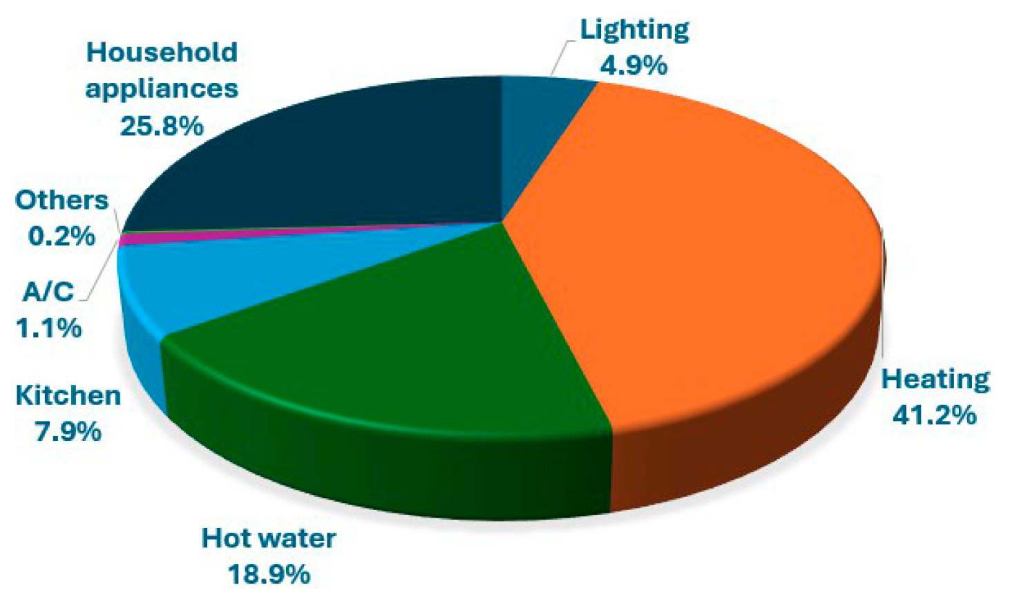
• Initial Consumption Values: The annual consumption values for each end use (Lighting, Heating, etc.) are given by the sum of the values for each month and are determined by the reference percentages (Figure 1).
• Monthly Constraints: For each month, the sum of the consumption across all end uses must match the total monthly consumption in kWh.
• Inconsistency Issue: If the initial consumption values for each category are too rigid or inflexible, they might not satisfy the total monthly consumption constraints.

To solve the system, some flexibility in the consumption values for each category must be allowed, permitting these values to change to fit the total monthly consumption better.

Mathematical Approach to the Solution

The mathematical approach proposed here is schematically depicted in Figure 2.

First, it is necessary to define the fluctuating variables for the various categories, which are the variables that can vary and do not maintain a fixed reference value. The first variable is heating consumption, initially estimated at 41.2% of the total annual energy consumption.

However, considering the mild winter temperatures of the study’s geographical context, this value might be overestimated and could be adjusted downward. The second variable is air conditioning consumption, estimated at 1.1% of the annual total. Given the high summer temperatures in the area, this value appears underestimated, so it may require an upward adjustment to reflect the more intense use during hotter months.

In addition to adjusting heating and air conditioning consumption, small adjustments might be necessary to balance the total consumption and make the model solvable. These adjustments include slightly modifying the values for household appliances. This category includes such devices as refrigerators, washing machines, dishwashers, etc., whose consumption is assumed to remain relatively constant throughout the year.

Following this, monthly constraints must be imposed. The system’s equations must ensure that the sum of all end uses for each month equals the total monthly consumption. The variable x_ij represents the consumption due to i in month j. Therefore, x_AC,July represents the air conditioning consumption in July. The variable C_j represents the sum of the consumption of all end uses in month j. Therefore, we can say that

$${{\displaystyle \sum }}_i{x}_{i,j}=C_j, \mathrm{for} \mathrm{each} \mathrm{month} j=1,2,\dots ,12$$

(1)

Another constraint is to ensure that the consumption for certain end uses remains constant over the various months. These categories are household appliances, hot water, and cooking. Given a fixed type of end use, x_ij must remain approximately constant for each month, and this can be expressed as follows:

x_i,j ≈ constant, for each month j

(2)

where i = household appliances, hot water, cooking

Another important consideration is related to lighting. The total consumption for lighting must be realistically distributed throughout the year, considering that it strongly depends on solar radiation and human habits. To achieve this, a binary variable L(t) can be modeled when lighting is needed. The first step is to analyze the solar radiation values (R(t)) for each hour of the day throughout the year. Each value R(t) represents solar radiation at a specific hour t, measured in W/m². A binary variable L(t) is introduced to represent whether the lighting is on or off at a given hour t. This variable takes the following values:

$$L\left(t\right)=\{\begin{array}{c}1, \mathrm{The} \mathrm{lighting} \mathrm{is} \mathrm{ON} \mathrm{at} \mathrm{time} t\\ 0, \mathrm{The} \mathrm{lighting} \mathrm{is} \mathrm{OFF} \mathrm{at} \mathrm{time} t\end{array}$$

(3)

The lighting activation depends on two main conditions:

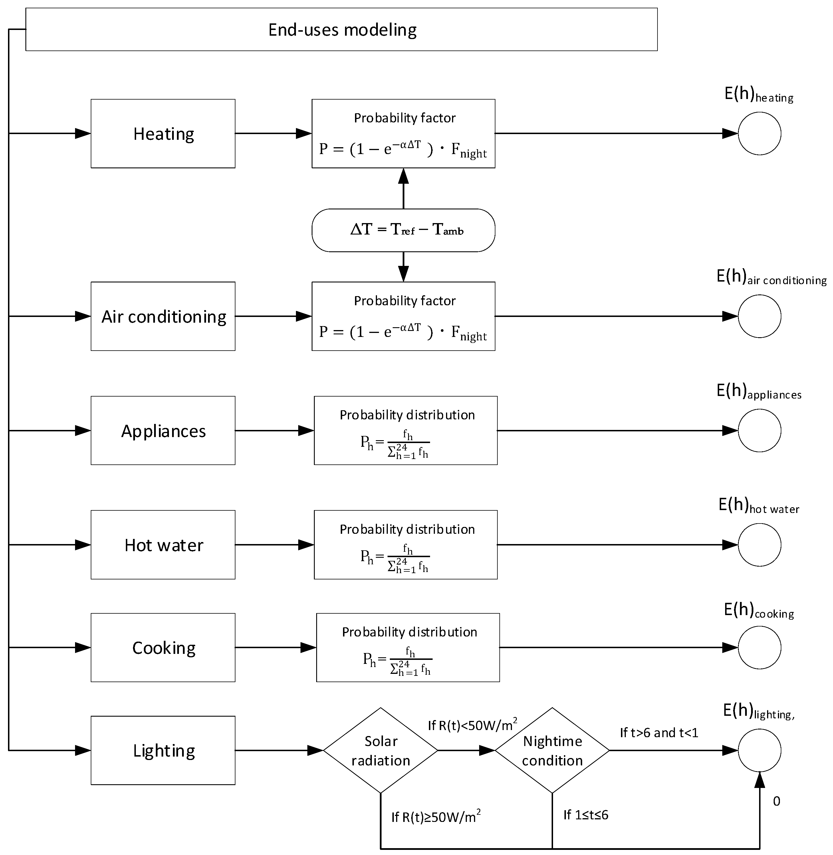
• Solar Radiation Condition: The lighting is on (L(t) = 1) if the solar radiation is below a certain threshold, R(t) < 50 W/m². This represents a low natural light condition.
• Nighttime Condition: Even if R(t) < 50 W/m², the lighting is off (L(t) = 0) during the nighttime hours (from 1:00 AM to 6:00 AM), assuming that people sleep and, therefore, do not need lighting. This time range has been assumed uniform for the whole annual period. However, it could be adjusted by considering the sunrise and sunset times throughout the year. Nevertheless, changing this time range would not significantly affect the final results.

Combining the two conditions, L(t) can be calculated as

$$L\left(t\right)=\{\begin{array}{c}1, \mathrm{if} R\left(t\right)<50 \mathrm{W}/{\mathrm{m}}^2 \wedge t\notin \left[1,6\right]\\ 0, \mathrm{otherwise} \end{array}$$

(4)

This expression changes to

$$L\left(t\right)=\{\begin{array}{c} 1, \mathrm{if} R\left(t\right)<50 \mathrm{W}/{\mathrm{m}}^2 \wedge (t>6 \vee t<1)\\ 0, \mathrm{if} R\left(t\right) \ge 50 \mathrm{W}/{\mathrm{m}}^2 \vee \left(1 \le t \le 6\right) \end{array}$$

(5)

The total lighting consumption for a given month is distributed over the hours when L(t) = 1. The variable T_i is defined, representing the total annual consumption of end-use i, which is given by the following sum:

$${{\displaystyle \sum }}_{\mathrm{j}}{\mathrm{x}}_{\mathrm{i},\mathrm{j}}=T_i,\mathrm{for} \mathrm{each} \mathrm{end} \mathrm{use} i$$

(6)

Knowing that the total annual consumption for lighting is T_Lighting, this value can be distributed on an hourly basis according to the number of hours the lighting is on during each month. If H_j is the total number of hours when L(t) = 1 for month j, the monthly consumption for lighting can then be calculated as follows

$$X_{Lighting,j}=\left({\displaystyle \frac{T_{Lighting}}{{{\displaystyle \sum }}_{j=1}^{12}{H}_j}}\right)·H_j \mathrm{for} \mathrm{each} \mathrm{month} j=1,2,\dots ,12$$

(7)

This approach ensures that the total annual lighting consumption is distributed proportionally based on the actual lighting needs each month, considering both solar radiation levels and nighttime hours.

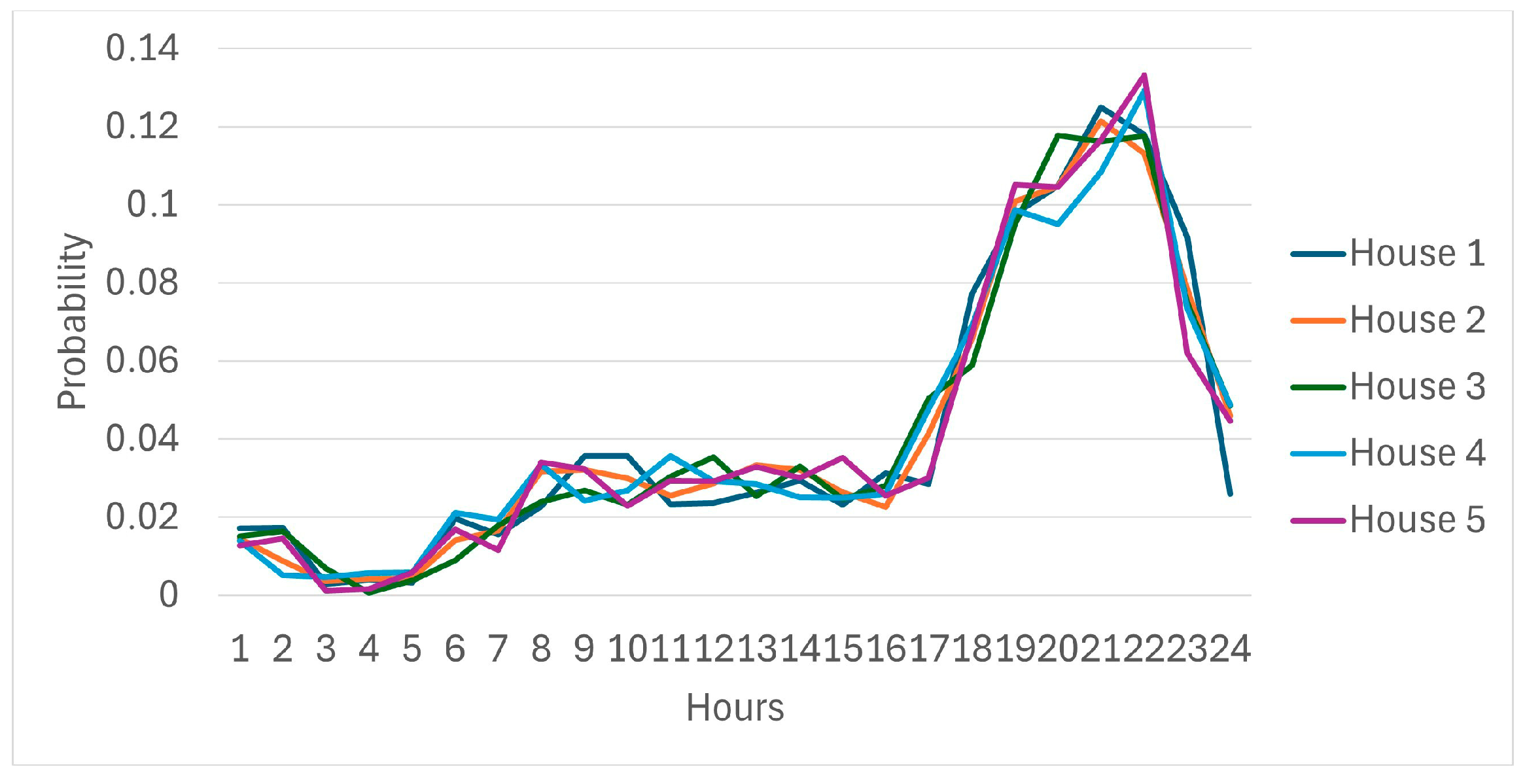
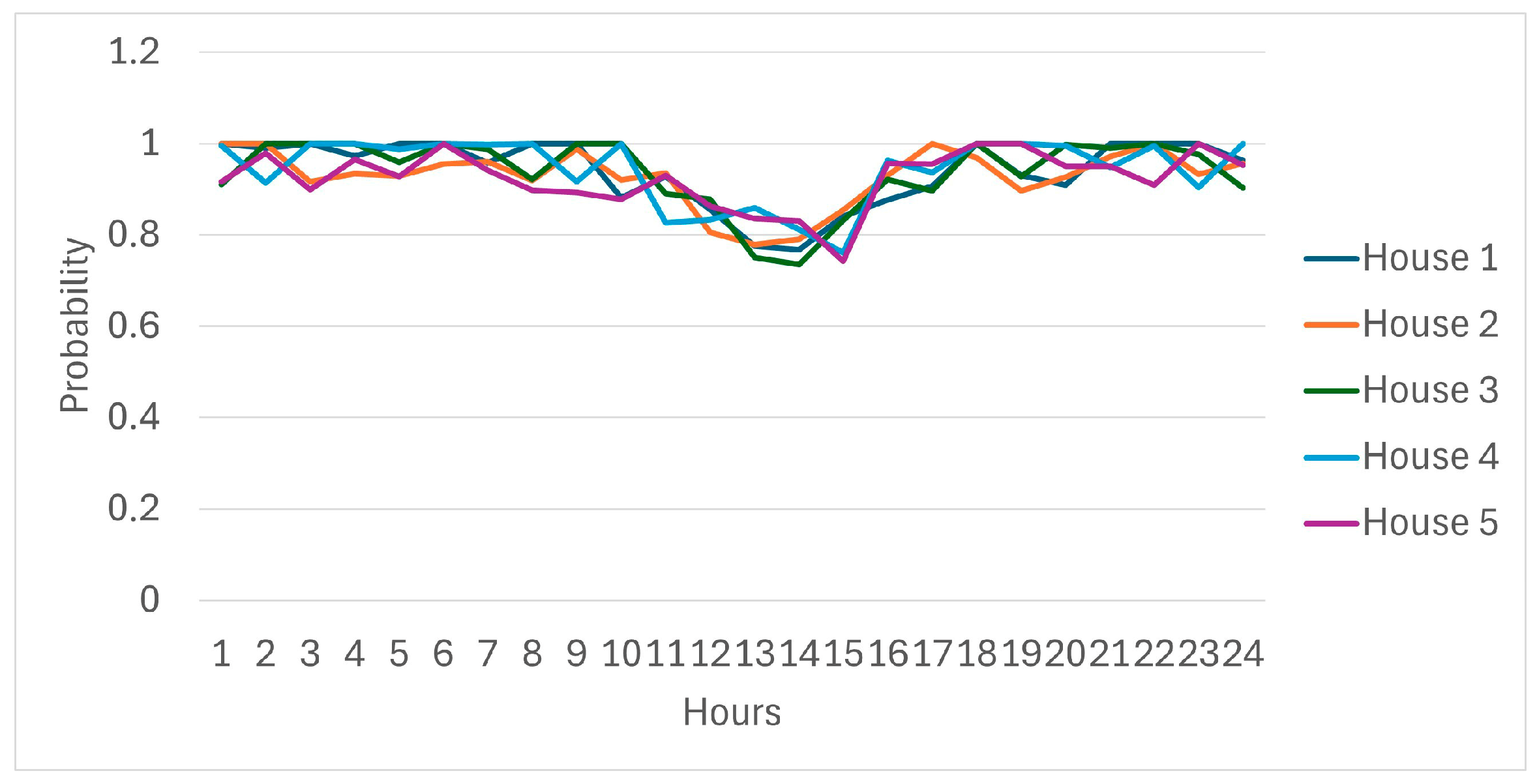
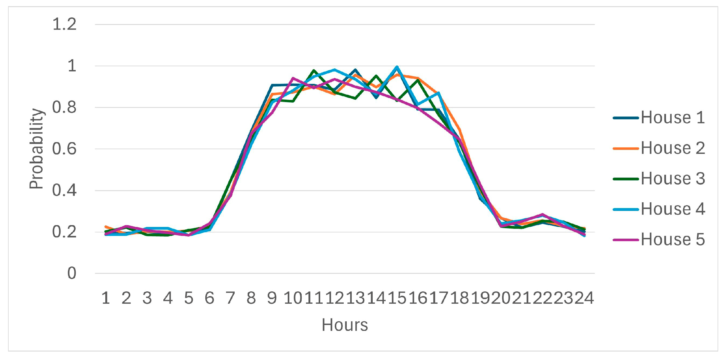
2.4. Identification of Consumption Patterns

The methodology continues with analyzing consumption patterns for each type of end-use. In this case, it is based on statistical data reported in the article [43], where the average consumption profiles of Spanish households were analyzed.

The study introduces a stochastic simulation model that utilizes the Survey of Time Use data from the National Statistics Institute of Spain (INE) [44]. This model allows for estimating the average profile of household electricity consumption based on the number of family members and the day of the week. Determining consumption profiles is a complex challenge due to the variability in household sizes, home occupancy, and the types of appliances used. The study employs ‘bottom-up’ models where specific data on individual households and their consumption are collected, and then this information is aggregated to provide a broader picture. Based on data from the SET survey, which provides information on the occupational behavior of households, the activity performed by each family member every ten minutes is correlated with energy consumption, assessing which appliances are used. In conclusion, the average consumption profiles for different time slots are presented. This data provides a solid basis for estimating the usage probabilities for each end-use, such as cooking, oven, lighting, washing machine, dishwasher, dryer, TV, and others, throughout the day.

To estimate the probability of use for each end-use throughout the day, the following steps were followed:

• For each graph related to appliance consumption, the maximum power value was identified and assigned a maximum usage relative frequency of 1 (100%). When there is no consumption, the power value is associated with a usage relative frequency of 0 (0%). In this way, a reference scale was created for each graph, which is useful for calculating relative frequencies for each time slot.
• The day was divided into hourly time slots. For each time slot, the resulting relative frequency range was calculated.
• The calculated range was taken as a reference to represent the variability in consumption. In fact, to introduce variability between different households, for each hour of the day and for each household, a random relative frequency value was generated within the calculated range. This allowed for the simulation of a more realistic and representative distribution of electricity consumption, reflecting the natural variability of consumer behavior based on home occupancy, the number of people present, and consumption variations related to whether the day is a weekday or holiday.
• This process was repeated for all end uses mentioned in the article [45].
• To obtain the probability of usage for each hour h, the value of the relative frequency f_h for each hour must be divided by the sum of all relative frequencies over the 24 h of the day:

$$P_h={\displaystyle \frac{f_h}{{{\displaystyle \sum }}_{h=1}^{24}{f}_h}}$$

(8)

This way, the total sum of the normalized probabilities will be 1, transforming the relative frequencies into a proper probability distribution.

The relative frequency indicates how often a particular appliance is used each hour compared to daily usage. This metric helps to reflect the variability of consumption behavior across different households or appliances. By normalizing these relative frequencies, probabilities that are easier to compare across different time slots or appliances can be obtained.

In the analysis of consumption patterns for the end uses described in the article, several appliances were considered, but estimates for heating, air conditioning, hot water, refrigerators, freezers, and standby were missing. Therefore, a different approach was adopted for these specific uses.

To estimate the probability of usage for heating and air conditioning, the following exponential probability function is used:

$$P=\left(1-{\mathrm{e}}^{-\alpha ∆T}\right) ·F_{night}$$

(9)

F_night is a factor that reduces the probability during nighttime hours. This reduction reflects the lower heating or air conditioning (AC) use during those hours. Essentially, it adjusts the probability model to account for the fact that heating and AC are typically used less at night, resulting in a lower overall probability of demand for these systems in those periods. This factor takes values from 0 and 1. In this case, an average value for Fnight of 0.6 has been obtained from 1 AM to 7 AM for heating, while this value was 0.3 from 1 AM to 8 AM in the winter.

This function was chosen because it represents a classic exponential model, allowing the probability to be expressed as a function of the temperature difference (∆T). The approach is justified because heating usage tends to be a non-linear response to the difference between the ambient temperature and a reference temperature, increasing rapidly as the temperature drops below a certain level. The ∆T for heating can be defined as follows:

∆T = T_ref − T_amb

(10)

where

• T_ref is the reference temperature (the temperature at which the respective heating or air conditioning systems are activated).
• T_amb is the ambient temperature measured at a specific time. The greater the difference ∆T, the higher the probability of heating usage. If T_amb > T_ref, meaning when the ambient temperature exceeds the reference temperature, ∆T = 0 is set, and thus the probability of heating usage becomes zero.

The approach used for air conditioning is similar to that of heating, with the difference that the calculation of ∆T follows the inverse relation:

∆T = T_amb − T_ref

(11)

In this case, the probability of air conditioning usage increases as the ambient temperature T_amb exceeds the reference temperature T_ref. If T_amb < T_ref, which means that the ambient temperature is lower than the reference temperature, ∆T = 0 is set, nullifying the probability of the use of air conditioning.

In the exponential function, the parameter α plays a crucial role in determining the sensitivity of the probability with respect to the temperature difference ∆T. In this case, after testing other options from 0 to 1.5 with a step of 0.1, α = 0.5 was chosen. When α was closer to zero, the sensitivity the demanded power to ∆T was very low, so that flatten load curve for this process was obtained and so, the underestimation of the real response of consumers with temperature. On the other side, when α was closer to 1 and higher, the probability to increase or reduce the power of this process was very sensitive to ∆T even for small temperature variations, quickly modifying the value of power. Therefore, an intermediate value of α was chosen, reflecting a moderate sensitivity to the increase in ∆T, which is consistent with the idea that the use of heating or air conditioning does not increase too abruptly but follows a more gradual pattern.

After calculating the probability of heating usage for each hour of the day in January and air conditioning usage for the month of July, as described previously, variability was introduced for all the households.

For each hour, instead of using a single calculated probability value P, a random probability value was generated within 90% to 110% of the initially calculated probability, meaning within the range [0, 9 · P; 1, 1 · P]. This allows the probability for each household to vary within this range, simulating diversity in consumption behavior across different houses.

After calculating the probability for each hour, the values were normalized. This means that all the probabilities for each hour were summed, and then each individual hour’s probability was adjusted by dividing it by this sum. This process ensures that the total sum of all hourly probabilities equals 1. Normalizing the values creates a comparable scale, allowing heating or air conditioning usage patterns to be easily compared with other end uses.

Regarding end uses such as refrigerators, freezers, and devices in standby mode, a nearly constant behavior over time was assumed. Since these appliances operate continuously and regularly, without significant variations throughout the day, a relative frequency between 80% and 100% was assumed. This reflects that these devices are generally active most of the time, with minimal variations in their operation. As a result, their contribution to energy consumption was considered relatively stable over 24 h, without significant peaks or drops compared to other, more variable end uses.

To analyze the hot water consumption pattern, the results from the study cited in [40] were used. Specifically, the relative frequency of domestic hot water usage at different times of the day was extracted.

Similarly to the approach used for other consumption estimates, normalization was applied to ensure that the sum of all probabilities across the hours equals 1. Furthermore, instead of using a single probability value for each time interval, a range introduced variability between households, allowing for a more realistic comparison of usage patterns across different households and time slots. For each time interval, a range between [0, 9 · P; 1, 1 · P] was considered, where P represents the probability calculated from the percentage of consumption indicated in the table. Only data related to weekdays were considered for this analysis.

2.5. Total Energy Consumption Across All Households

To estimate the hourly total consumption in kWh for a number C of households related to each end use, the following procedure was followed:

• Construction of the probability matrix: For each end use, a matrix was created where
  • The rows correspond to the 24 h of the day (h = 1, 2, …, 24).
  • The columns represent the households (i = 1, 2, …, C).
  Each cell P_h,i of the matrix contains the probability that the end use is activated at hour h in house i.
• Sum of probabilities for each hour: For each hour of the day, the sum of probabilities across all households was calculated. The sum of probabilities for hour h is given by

  $$P_{sum}\left(h\right)={{\displaystyle \sum }}_{i=1}^c{P}_{h,i}$$

  (12)
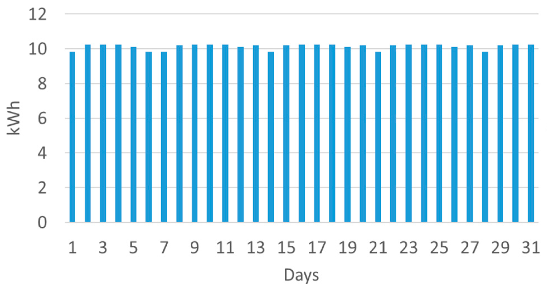
• Determination of total daily consumption: The total daily consumption for a single household is known from the TSO data. This value, denoted as E_{tot_house}, is multiplied by C to obtain the total daily consumption for all the households, assuming that the consumption is approximately the same across all households:

  $$E_{toc\_C}=C . E_{tot\_house}$$

  (13)

  This value represents the households’ total consumption on a specific day (e.g., January 1st).
• Application of the ratio of consumption for each end use: Each end use has its ratio of consumption based on the month and the type of use. This value, denoted as %(M), represents the share of energy allocated to that specific end use in month M. Therefore, the specific daily consumption for that end use is given by

  $$E_{end\_use}=E_{tot\_C}·\%\left(M\right)$$

  (14)
• Distribution of consumption for each hour: To obtain the hourly E(h) related to each end use, the following calculation was used:

  $$E\left(h\right)={\displaystyle \frac{P_{sum}\left(h\right)}{{{\displaystyle \sum }}_{h=1}^{24}{P}_{sum}\left(h\right)}} · E_{end\_use}$$

  (15)

  where
  • P_sum(h) is the sum of the probabilities for hour h across all households.
  • ${\displaystyle \sum }_{h=1}^{24}{P}_{sum}\left(h\right)$ represents the total sum of probabilities over all hours and all households.
  • E_{end_use} is the total daily consumption for the specific end-use calculated earlier.
• Results: By repeating this calculation for all hours (h = 1, 2, …, 24), the kWh consumed for each hour of the day for the given end use is obtained. To calculate the total consumption for each hour considering all end uses, the energy consumption for each end use u at the same hour h is summed. Therefore, the total hourly consumption E_total(h) at the h-th hour of the day is given by

  $$E_{total}\left(h\right)={{\displaystyle \sum }}_{u\in U}{E}_u\left(h\right)$$

  (16)

  where
  • E_total(h) is the total consumption for all households at hour h, considering all end uses.
  • E_u(h) is the hourly consumption for end use u at hour h.
  • U is the set of all end uses (e.g., heating, lighting, hot water, etc.).

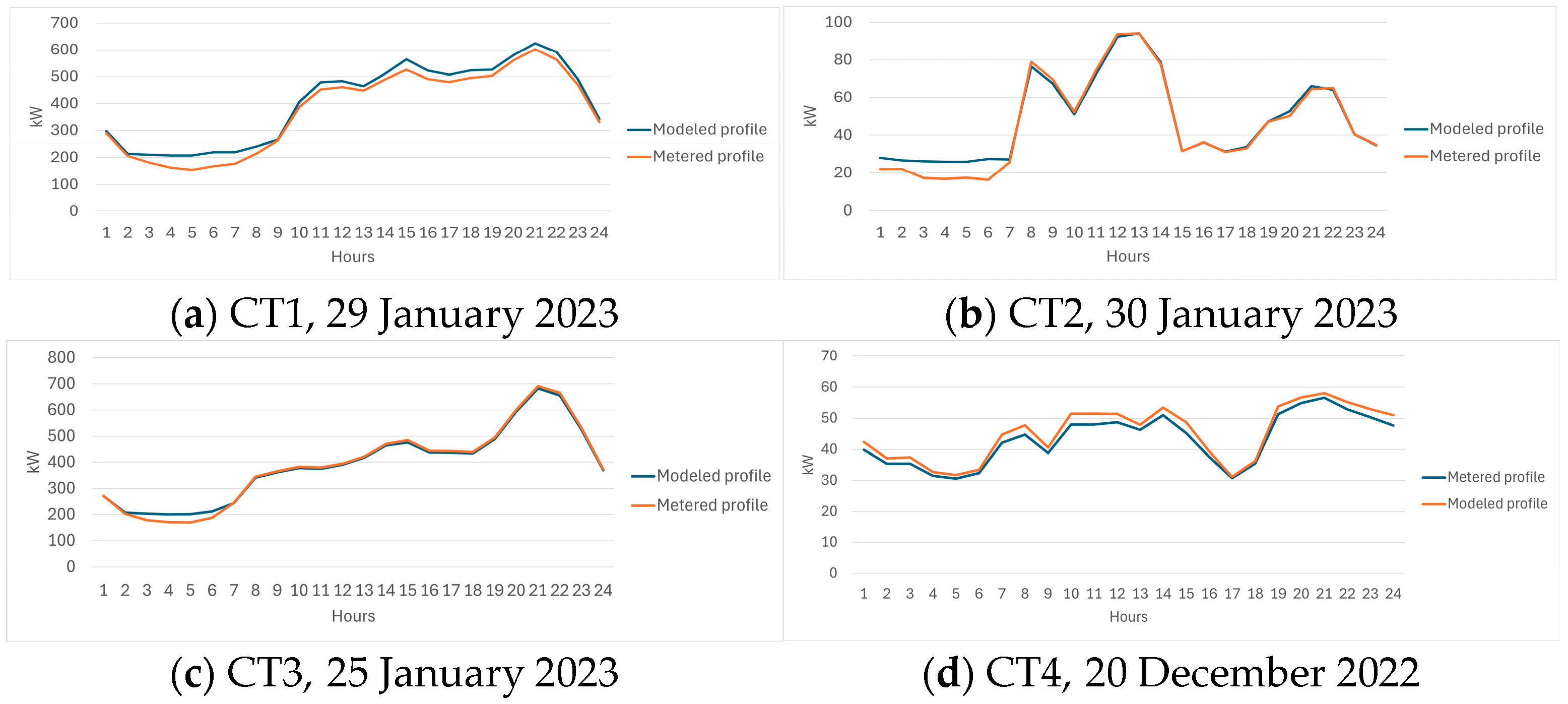
3. Case Study

Applying the Methodology to Real Data Profile Disaggregation

This methodology will be applied to real cases, using actual consumption data provided by the electricity company. Typically, they provide aggregated consumption data from the transformation centers to which the consumers are connected. Therefore, it is necessary to select the specific dates of interest for analysis.

To assess the amount of flexible consumption, it is necessary to know the consumption trends for the end uses of interest: washing machines, dishwashers, dryers, heating, air conditioning, and hot water. Since the patterns of these specific consumptions are not known beforehand, they must be estimated based on the total consumption patterns and the probability values obtained from statistical analysis. Next, the procedure used to reconstruct disaggregated consumption profiles by end-use is presented, followed by the results obtained from the flexibility analysis. The method can be described with the following points:

• Construction of the probability matrix: For each end use, a probability matrix P_{end_use}(h, i) is constructed, where
  • h = 1, 2, …, 24 are the hours of the day (rows of the matrix).
  • i = 1, 2, …, C represents the consumers for each transformation center (columns of the matrix).
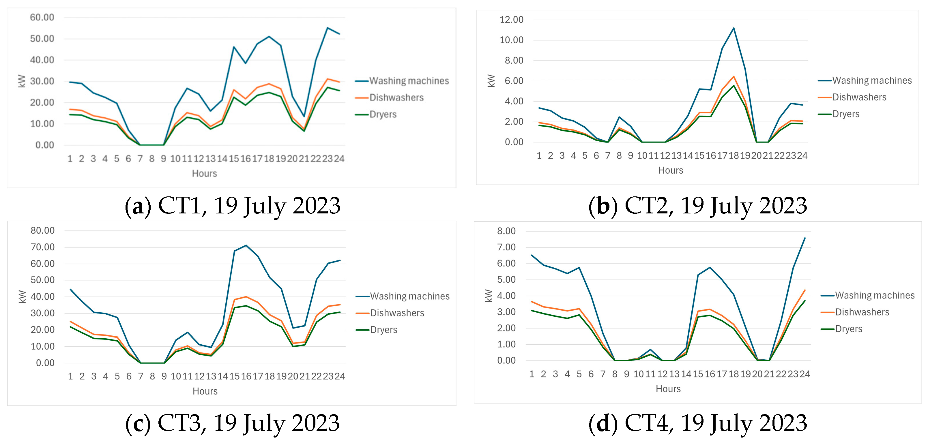
• Distinction between modified and non-modified end uses: The distinction is made between modified end uses (washing machine, dishwasher, dryer, and hot water) and non-modified end uses (all others). The probability matrices for non-modified end use remain as initially estimated. However, the probability matrices for the modified end uses are adjusted based on the difference between the real measured data and the sum of the non-modified consumption. This ensures that the consumption trends for the modified end uses align with the measured data, providing a more accurate reflection of their actual behavior.
• Adjustment based on the difference between total consumption and non-modified end uses: First, the total consumption E_metered(h) for each hour is taken from measured data. Then, the sum of the consumption for all non-modified end uses (i.e., all except washing machine, dishwasher, dryer, and hot water) is subtracted from the total real measured consumption to isolate the portion related to the modified end uses. The non-modified consumption, E_{total_non_mod}(h), is represented as follows:

  E_{total_non_mod}(h) = E_metered (h) − E_{washing machine}(h) + E_dishwasher(h) + E_dryer(h) + E_{hot water}(h)

  (17)
  The remaining consumption for the modified end uses is then:

  E_{total_mod}(h) = E_metered(h) − E_{total_non_mod}(h)

  (18)
• Calculation of new consumption ratios: Since the non-modified consumption has been subtracted, the consumption ratios for the modified end uses are recalculated. The new consumption ratios (c.ratio_end-use-new), for each end-use, are:

  $$c.rati{o}_{end-use-new}={\displaystyle \frac{c.rati{o}_{end-use}·\left(1-c.rati{o}_{non-mod}\right)}{100}}$$

  (19)
• Calculation of kWh for modified end uses: Once the new ratios for modified end uses are determined, the kWh E_{end_use}(h) for each modified end-use is calculated as:

  E_{end_use}(h) = E_{total_mod}(h) · c.ratio_end-use-new

  (20)
• Calculation of P_sum for modified end uses: The sum of probabilities for each hour P_sum(h) for modified end uses is calculated using the following formula:

  P_sum(h) = ∑ P_{end_use}(h) · c.ratio_{end_use_new}

  (21)
• Calculation of new hourly probability for modified end uses: Once P_sum(h) is obtained for each hour, the new probability P_{end_use_new}(h) is calculated by dividing P_sum(h) by the number of consumers C:

  $$P_{\mathit{\text{end\_use\_new}}}\left(h\right) {\displaystyle \frac{P_{sum}\left(h\right)}{C}}$$

  (22)
  Additionally, it is essential to verify that the following condition holds, ensuring that the total sum of the matrix P_{end_use} remains constant:

  $${{\displaystyle \sum }}_{h=1}^{24}{{\displaystyle \sum }}_{i=1}^c{P}_{end\_use}\left(h,i\right)=P_{total}$$

  (23)
  Maintaining P_total constant is crucial to preserving the coherence of the model and adhering to the principle of conservation of the probabilistic phenomenon.
• Imposing variability: To introduce variability in the probability for each hour h and each consumer i, the value of P_{end_use_new}(h, i) will range between 90% and 110% of P_{end_use_new}(h), i.e.,

  P_{end_use_new}(h, i) ∈ [0.9 · P_{end_use_new}(h), 1.1 · P_{end_use_new}(h)]

  (24)
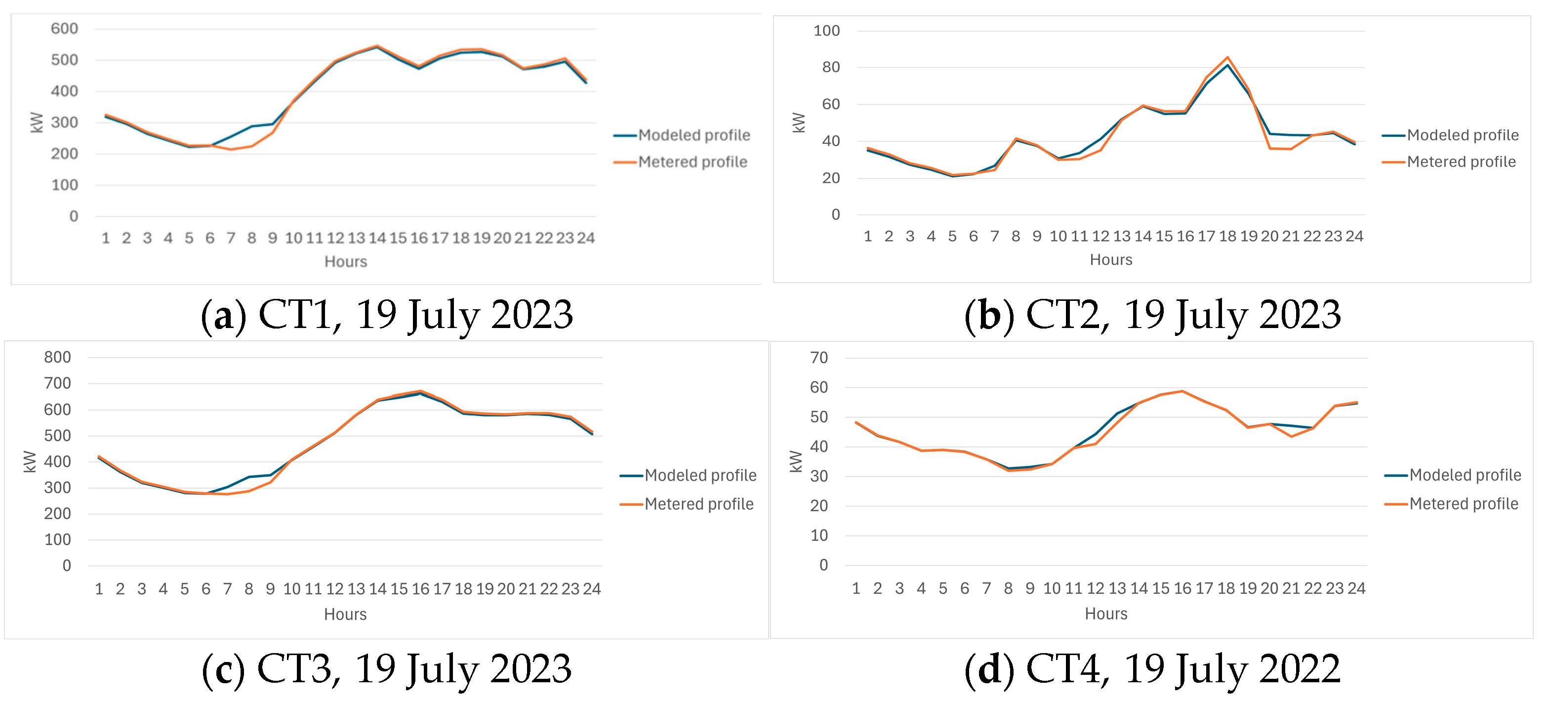
• Evaluation of the percentage error: The percentage error is calculated for each hour h of the day. The formula for the percentage error is given by

  $$Error\left(h\right)={\displaystyle \frac{E_{metered}\left(h\right) – E_{modeled}\left(h\right)}{E_{metered}\left(h\right)}}·100$$

  (25)

  where E_metered(h) represents the measured consumption and E_modeled(h) represents the modeled consumption, calculated as

  $$E_{modeled}\left(h\right)=E_{total\_non\_mod}\left(h\right)+E_{washing machine}\left(h\right)+E_{dishwasher}\left(h\right)+E_{dryer}\left(h\right)$$

  (26)

The described procedure, which is based on the difference between the real measured values (E_metered(h)) and the consumption for which the previously assumed probabilities are not modified (E_{total_non_mod}(h)), allows for the calculation of new probability values for flexible end uses. In this way, it is possible to identify the hours in which the probability of using a specific end use is higher than in other hours by leveraging the difference between the profiles. The goal is to ensure that the modeled curve (E_modeled(h)) gets as close as possible to the curve of the real measured data (E_metered(h)), minimizing the prediction error.

4. Discussions and Results

4.1. Consumption Analysis

The annual consumption graph (Figure 3) indicates that energy usage peaks during the winter and summer, with January and July showing the highest values, respectively. In contrast, spring and autumn exhibit more moderate consumption levels. The analysis of monthly consumption patterns (Figure 4) shows that daily energy usage remains relatively stable each month, with no significant variations between weekdays and weekends. This observation highlights the consistent nature of residential energy behavior, irrespective of the day of the week. Furthermore, the daily consumption graph for January (Figure 5) reveals two distinct peaks: one around midday and another in the evening. These peaks reflect typical residential routines and are critical for identifying the hours of maximum energy demand, which is a key factor in flexibility evaluation.

4.2. Consumption Characterization

At the end of analyzing and optimizing energy consumption, a solution is reached that reflects the actual needs and climatic conditions of the geographical context in which the study is conducted. Below, Figure 6 shows the annual percentage values. Specifically, the percentage value related to heating has been reduced to 20.24%. In comparison, the air conditioning value has increased to 12.96%, more accurately reflecting the high consumption during the hot summer months. Additionally, there has been a slight increase in the consumption of household appliances to maintain an overall balance in consumption.

The percentage values for each end use and each month are presented in

Table 1. Energy consumption ratios for each end use and for each month (a).

	Jan	Feb	Mar	Apr	May	Jun
Lighting	5.70%	5.61%	4.98%	4.57%	4.06%	4.86%
Heating	36.59%	35.38%	35.20%	25.28%	7.57%	0.00%
Hot water	21.66%	18.93%	18.27%	21.46%	25.42%	15.99%
Kitchen	6.40%	7.10%	7.63%	8.97%	9.38%	11.22%
Air conditioning	0.00%	0.00%	0.00%	0.00%	6.87%	19.66%
Others	0.21%	0.18%	0.20%	0.23%	0.27%	0.27%
Television	2.76%	3.41%	3.04%	3.55%	3.83%	4.34%
Freezers	1.32%	1.41%	1.52%	1.68%	2.11%	2.17%
Refrigerators	6.39%	7.09%	7.63%	8.96%	10.62%	10.88%
Oven	1.78%	1.92%	2.07%	2.43%	2.89%	2.42%
Washing machines	5.81%	6.76%	6.87%	8.07%	9.45%	10.11%
Dishwashers	3.65%	4.36%	4.30%	5.05%	5.99%	6.19%
Computers	1.75%	1.89%	1.85%	2.16%	2.57%	2.66%
Dryers	3.37%	3.49%	3.78%	4.43%	5.26%	5.41%
Stand-by	2.60%	2.46%	2.67%	3.13%	3.71%	3.83%

and in

Table 2. Energy consumption ratios for each end use and for each month (b).

	Jul	Aug	Sep	Oct	Nov	Dec
Lighting	3.59%	4.23%	5.57%	5.22%	6.62%	4.99%
Heating	0.00%	0.00%	7.19%	21.69%	30.52%	34.21%
Hot water	13.16%	13.12%	21.23%	22.32%	18.71%	23.12%
Kitchen	7.54%	7.74%	8.88%	9.33%	7.82%	6.82%
Air conditioning	44.40%	42.69%	17.76%	0.00%	0.00%	0.00%
Others	0.14%	0.20%	0.23%	0.24%	0.20%	0.17%
Television	2.38%	2.13%	3.53%	3.72%	3.90%	3.25%
Freezers	1.45%	1.54%	1.71%	1.86%	1.56%	1.36%
Refrigerators	7.53%	7.73%	8.87%	9.32%	7.82%	6.82%
Oven	1.99%	2.09%	2.40%	2.53%	2.50%	1.85%
Washing machines	6.73%	6.37%	7.98%	8.40%	7.24%	6.15%
Dishwashers	3.82%	4.15%	5.00%	5.26%	4.41%	3.85%
Computers	1.77%	1.48%	2.14%	2.25%	1.89%	1.65%
Dryers	3.30%	3.83%	4.39%	4.61%	4.07%	3.37%
Stand-by	2.20%	2.71%	3.10%	3.26%	2.73%	2.39%

below. These values represent the estimation of the annual energy consumption for each category, optimized to balance the overall energy demand without compromising daily functionality. This approach allows us to meet the monthly energy constraints and adapt to the specific seasonal and behavioral dynamics of the users.

As can be seen from the obtained values, the consumption of kitchen appliances, standby, and refrigerators remains almost constant throughout the year. Lighting shows lower values during the summer months. Heating and cooling consumption have zero values during the months when they are not used. Heating is absent in the summer, while air conditioning does not appear in the winter.

4.3. Identification of Consumption Patterns

The following graphs show the probability trends for different end uses; as an example, five typical houses have been used, but the methodology has been applied to all the houses that make up each of the transformation centers mentioned:

The highest probability to use lighting, as shown in Figure 7, is from the sunset to the time when users go to sleep. Therefore, the curve shows a peak from approximately 18:00 to 23:00. Consumption is almost zero during night and starts rising between 6:00 and 7:00, when users initiate their daily activity. Regarding the probability of using the kitchen, shown in Figure 8, there are two peaks during the day, which correspond times in which users are preparing lunch and dinner. Regarding acclimatization end used, the probability of using the heating (Figure 9) is higher when there is no sun, while air conditioning (Figure 10) is more likely to be used during the central hours of the day.

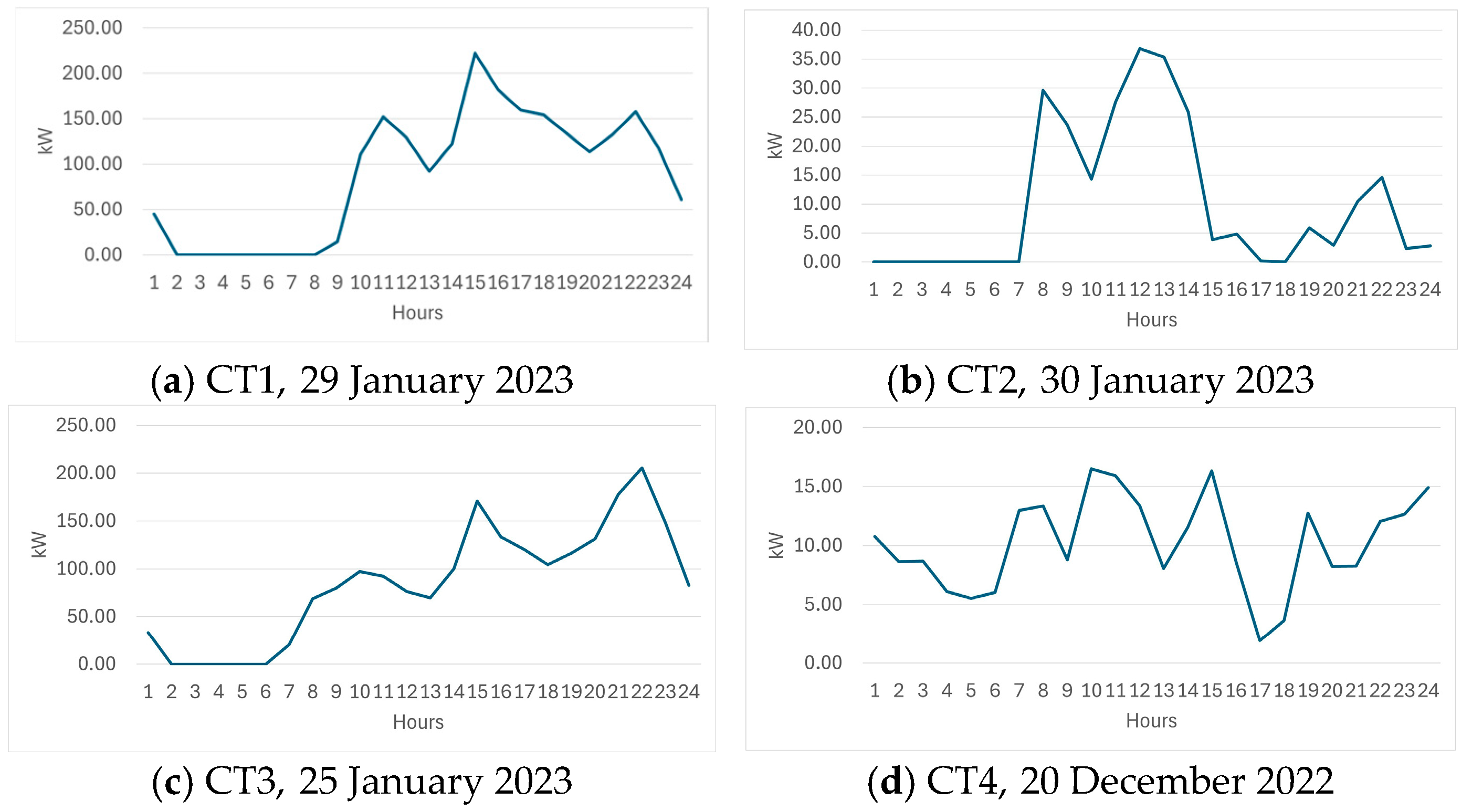
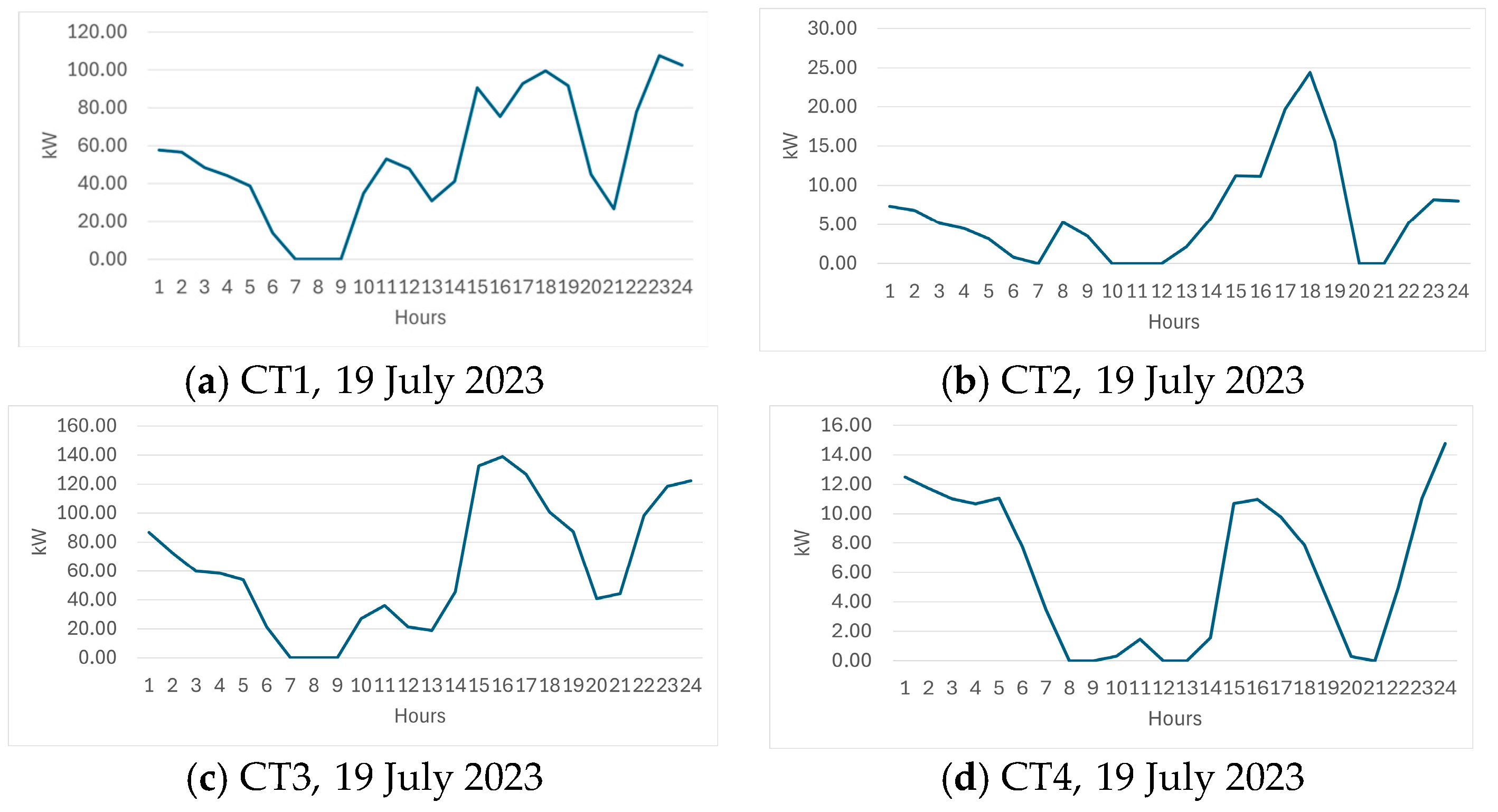
4.4. Applying the Methodology to Real Data and Profile Disaggregation

The methodology was applied to four transformer centers (CT1, CT2, CT3, CT4) for two significant dates: one in winter and one in summer, when consumption peaked. The results obtained are presented below. So, Figure 11 and Figure 12 show the consumption in winter and summer of considered CTS.

The RMSE values for the four transformation centers indicate a general trend of higher errors in the winter compared to the summer. Specifically, for CT1, the RMSE is 13.59% in the winter and 7.55% in the summer. Similarly, CT10 exhibits the highest discrepancies, with an RMSE of 24.06% in winter and 12.49% in summer. In contrast, CT19 and CT158 show lower error levels, with RMSE values of 6.56% and 5.10% in the winter and 4.85% and 2.76% in the summer, respectively. These results suggest that the model performs better during the summer, significantly reducing deviations from the actual consumption patterns. This fact could be justified by a more intensive utilization of the air conditioning due to the high temperatures in the summer, reaching usually more than 30 °C, while softer winters, where temperature rarely goes down below 5 °C, produce greater variability in the use of heating.

It should be taken into account that curves shown in Figure 11 and Figure 12 under the label “Metered profile” were provided by the electric distribution company, and so they were actually coming from real measurements at the transformation center (CT) level. Measurements at the household level were not available. However, the four transformation centers considered for this study were selected as most of consumers connected (96%) are residential. Validation was performed comparing the measured demand on each CT (assuming that all connected consumers were residential) and the sum of end use profiles modeled according to the proposed methodology, based on probabilities. Therefore, one of the most significant sources of uncertainty is the real power demanded by households compared to the total demand of the CT.

The disaggregated consumption by end use for the washing machine, dishwasher, and dryer are shown in Figure 13 and Figure 14.

The disaggregated consumption by end use for hot water is shown in Figure 15 and Figure 16.

Previous figures show the load profile for a typical day in winter and summer corresponding to end uses that can provide flexibility to the end-user consumption. Indeed, the obtained profiles present diverse power peaks that represent the possibility to shift power from these periods to others. Therefore, with the appropriate coordination provided by load aggregators, end-users could schedule their activities in some specific periods in order to modify their usual pattern of consumption.

5. Conclusions

This study has presented a methodology for the disaggregation of residential energy consumption, a key step in advancing the detailed assessment of the potential for demand flexibility. Throughout the research, it has been shown that the ability to break down energy consumption into its different components (such as heating, air conditioning, and appliances) provides a more precise and more accurate picture of consumption patterns, facilitating more efficient management of energy resources. Understanding how each device or system contributes to total consumption makes it possible to identify key areas where flexibility can be applied to improve overall energy efficiency. This methodology provides a robust framework for analyzing the impact of flexibility on demand reduction during periods of high load or at times of high variability in renewable energy supply. Although this methodology has been validated using real data from the distribution network of a Spanish municipality, it is essential to highlight that its application is not limited to this geographical area. Its flexibility and adaptability allow it to be applied to regions with varied climatic characteristics and consumption patterns. This is especially relevant in the current energy transition context, where the incorporation of renewable energy technologies is growing, and an improved capacity to manage the variability and uncertainty associated with these energy sources is required. In this sense, the methodology developed has the potential to become a key tool in planning and managing residential electricity demand in different environments and markets.

A fundamental aspect that has emerged throughout the study is the importance of accurately disaggregating household energy consumption to identify sources of flexibility. In this respect, characterizing the leading energy end uses, such as heating systems, air conditioning, and household appliances, is essential for optimizing consumption according to energy availability and prices. For example, household appliances such as washing machines, dryers, and ovens can be adjusted to operate at times of lower demand, which benefits the household in terms of energy savings and contributes to the electricity grid’s stability. In addition, this unbundling allows for a deeper analysis of energy flexibility in the residential sector, which can lead to improved planning of energy generation and storage capacity. While demand flexibility has traditionally been more focused on the industrial and commercial sectors, the residential sector has proven to be equally relevant due to its size and heterogeneity. In this sense, a detailed analysis of household consumption patterns could reveal new flexibilization opportunities that, until now, have been underestimated or not sufficiently exploited. This would open the door to implementing more effective strategies to balance supply and demand, especially in the increasing penetration of intermittent renewable energies such as solar and wind. Accurate disaggregation of energy consumption also improves the effectiveness of demand-side management strategies, allowing households to be more proactive in optimizing their consumption. For example, detailed analysis of consumption patterns and identification of flexible end uses enables the development of incentive programs that encourage consumer participation in demand response. Such programs could reward users for reducing their consumption during peak demand or shifting it to times of low demand. This benefits them economically and helps to balance the electricity grid and reduce greenhouse gas emissions associated with generating energy from non-renewable sources.

This study has also highlighted the importance of data in the transition to a more sustainable energy system. Using accurate, real-time data is critical to improving the energy system’s efficiency and enabling smarter, more resilient electricity grids. As the integration of connected devices and automation technologies in homes moves forward, new opportunities will open up to optimize energy consumption and improve demand flexibility. However, this also presents challenges related to data privacy and interoperability between different devices and platforms.

Finally, identifying and characterizing energy end uses in households is critical to support the transition towards sustainable energy systems. By enabling greater customization of demand-side management strategies, this approach helps to reduce energy consumption efficiently and reduces the carbon footprint of households. In addition, optimizing energy consumption in the residential sector directly impacts reducing dependence on non-renewable energy sources, which is critical to achieving European and global climate targets. Limitations of the study are mainly related to the distribution of energy consumption by end uses, which may vary from some regions to others. Indeed, the methodology could be applied to other regions with different climates or consumption patterns by modifying the characterization which has been depicted in Section 2.3. The characterization applied to other areas could be based on existing research available in bibliography or by means of additional pilots to identify how electricity is divided into end uses. An additional limitation could be given by socioeconomic differences among areas as energy consumption by end uses depends not just on a geographic position but also on the electrification level, kinds of appliances, and acclimatization technologies (such as cooling and heating devices) that are used in households. Therefore, the location of the area where this study has been applied makes results specifically applicable to countries in southern Europe and similar geographic areas.

6. Future Research

Future lines of research and work can be envisaged based on the initial steps of the flexibility tool methodology developed in this study, which focuses on the disaggregation of residential energy consumption. While this work primarily addresses the disaggregation process, it lays the foundation for future assessments of demand-side flexibility. Firstly, the methodology’s scalability at the national level could be investigated and adapted to different consumer profiles and operating conditions in other regions of Spain. Furthermore, it would be essential to assess the impact of demand flexibility on integrating renewable energies, maximizing their incorporation into the electricity system, and reducing intermittency issues.

Future work could also explore how different socio-economic groups react to demand-side management strategies, identifying potential technological and economic barriers. Additionally, modeling long-term demand flexibility, accounting for aging equipment, and evolving consumption patterns, would provide further insights. From a policy perspective, developing regulatory strategies and economic incentives to encourage residential participation in flexibility programs is essential. Optimizing the flexibility tool through artificial intelligence and big data techniques could further enhance predictions of demand behavior and personalize energy management strategies. Lastly, exploring the interaction between demand flexibility and energy storage solutions, as well as extending the analysis to other sectors, such as commercial or industrial, would allow for a broader evaluation of flexibility potential across the energy system.

References

1. European Commission. Directorate-General for Climate Action, Going Climate-Neutral by 2050—A Strategic Long-Term Vision for a Prosperous, Modern, Competitive and Climate-Neutral EU Economy; Publications Office: Brussels, Belgium, 2019. [Google Scholar]
2. Vargas-Salgado, C.; Borràs, I.M.; Alcazar-Ortega, M.; Montuori, L. Floating PV Solar-Powered Systems: Design applied to an irrigators community in the Valencia Region—Spain. In Proceedings of the 2020 Global Congress on Electrical Engineering (GC-ElecEng), Valencia, Spain, 4–6 September 2020; pp. 88–95. [Google Scholar]
3. Jakučionytė-Skodienė, M.; Liobikienė, G. Climate change concern, personal responsibility and actions related to climate change mitigation in EU countries: Cross-cultural analysis. J. Clean. Prod. 2021, 281, 125189. [Google Scholar] [CrossRef]
4. Montuori, L.; Alcázar-Ortega, M.; Álvarez-Bel, C.; Domijan, A. Integration of renewable energy in microgrids coordinated with demand response resources: Economic evaluation of a biomass gasification plant by Homer Simulator. Appl. Energy 2014, 132, 15–22. [Google Scholar] [CrossRef]
5. Erenoğlu, A.K.; Şengör, İ.; Erdinç, O.; Taşcıkaraoğlu, A.; Catalão, J.P.S. Optimal energy management system for microgrids considering energy storage, demand response and renewable power generation. Int. J. Electr. Power Energy Syst. 2022, 136, 107714. [Google Scholar] [CrossRef]
6. Panuschka, S.; Hofmann, R. Impact of thermal storage capacity, electricity and emission certificate costs on the optimal operation of an industrial energy system. Energy Convers. Manag. 2019, 185, 622–635. [Google Scholar] [CrossRef]
7. Rodriguez-Garcia, J.; Ribo-Perez, D.; Alvarez-Bel, C.; Penalvo-Lopez, E. Maximizing the Profit for Industrial Customers of Providing Operation Services in Electric Power Systems via a Parallel Particle Swarm Optimization Algorithm. IEEE Access 2020, 8, 24721–24733. [Google Scholar] [CrossRef]
8. Montuori, L.; Alcázar-Ortega, M. Demand response strategies for the balancing of natural gas systems: Application to a local network located in The Marches (Italy). Energy 2021, 225, 120293. [Google Scholar] [CrossRef]
9. Heffron, R.; Körner, M.-F.; Wagner, J.; Weibelzahl, M.; Fridgen, G. Industrial demand-side flexibility: A key element of a just energy transition and industrial development. Appl. Energy 2020, 269, 115026. [Google Scholar] [CrossRef]
10. Acer. Demand Response and Other Distributed Energy Resources: What Barriers Are Holding Them Back? 2023 Market Monitoring Report. 2023. Available online: www.acer.europa.eu (accessed on 24 March 2025).
11. Tuomela, S.; Tomé, M.D.C.; Iivari, N.; Svento, R. Impacts of home energy management systems on electricity consumption. Appl. Energy 2021, 229, 117310. [Google Scholar] [CrossRef]
12. Olawale, O.W.; Gilbert, B.; Reyna, J. Residential Demand Flexibility: Modeling Occupant Behavior using Sociodemographic Predictors. Energy Build. 2022, 262, 111973. [Google Scholar] [CrossRef]
13. Bahramara, S. Robust Optimization of the Flexibility-constrained Energy Management Problem for a Smart Home with Rooftop Photovoltaic and an Energy Storage. J. Energy Storage 2021, 36, 102358. [Google Scholar] [CrossRef]
14. Vellei, M.; Dréau, J.L.; Abdelouadoud, S.Y. Predicting the demand flexibility of wet appliances at national level: The case of France. Energy Build. 2020, 2014, 109900. [Google Scholar] [CrossRef]
15. D’hulst, R.; Labeeuw, W.; Beusen, B.; Claessens, S.; Deconinck, G.; Vanthournout, K. Demand response flexibility and flexibility potential of residential smart appliances: Experiences from large pilot test in Belgium. Appl. Energy 2015, 155, 79–90. [Google Scholar] [CrossRef]
16. Stamminger, A.S.R. Load profiles and flexibility in operation of washing machines and dishwashers in Europe. Int. J. Consum. Stud. 2017, 41, 178–187. [Google Scholar] [CrossRef]
17. Dortans, C.; Jack, M.W.; Anderson, B.; Stephenson, J. Lightening the load: Quantifying the potential for energy-efficient lighting to reduce peaks in electricity demand. Energy Effic. 2020, 13, 1105–1118. [Google Scholar] [CrossRef]
18. Utama, C.; Troitzsch, S.; Thakur, J. Demand-side flexibility and demand-side bidding for flexible loads in air-conditioned buildings. Appl. Energy 2021, 285, 116418. [Google Scholar] [CrossRef]
19. Lakshmanan, V.; Sæle, H.; Degefa, M.Z. Electric water heater flexibility potential and activation impact in system operator perspective—Norwegian scenario case study. Energy 2021, 236, 121490. [Google Scholar] [CrossRef]
20. Hoyne, S.; Breen, M.; Campbell, A.; Miraglia, E.; Hurley, J. Decarbonisation of Residential Heating and Cooling: The Heat Pump Challenge; Publications Office of the European Union: Brussels, Belgium, 2024; ISSN 978-92-897-2437-1. [Google Scholar]
21. Widera, B. Energy and Carbon Savings in European Households Resulting from Behavioral Changes. Energies 2024, 17, 16. [Google Scholar] [CrossRef]
22. Zehir, M.A.; Bagriyanik, M. Demand Side Management by controlling refrigerators and its effects on consumers. Energy Convers. Manag. 2012, 64, 238–344. [Google Scholar] [CrossRef]
23. Alsharif, A.; Ahmed, A.A.; Khaleel, M.M.; Alarga, A.S.D.; Jomah, O.S.M.; Imbayah, I. Comprehensive State-of-the-Art of Vehicle-To-Grid Technology. In Proceedings of the IEEE 3rd International Maghreb Meeting of the Conference on Sciences and Techniques of Automatic Control and Computer Engineering (MI-STA), Benghazi, Libya, 21–23 May 2023; pp. 530–534. [Google Scholar]
24. Plaum, F.; Ahmadiahangar, R.; Rosin, A.; Kilter, J. Aggregated demand-side energy flexibility: A comprehensive review on characterization, forecasting and market prospects. Energy Rep. 2022, 8, 9344–9362. [Google Scholar] [CrossRef]
25. Raineri, R. Power Shift: Decarbonization and the New Dynamics of Energy Markets. Energies 2025, 18, 752. [Google Scholar] [CrossRef]
26. ENEFIRST. Using Time-of-Use tariffs to Engage Customers and Benefits the Power System; European Union: Brussels, Belgium, 2019. [Google Scholar]
27. Amissah, J.; Abdel-Rahim, O.; Mansour, D.E.A.; Bajaj, M.; Zaitsev, I.; Abdelkader, S. Developing a three stage coordinated approach to enhance efficiency and reliability of virtual power plants. Sci. Rep. 2024, 14, 13105. [Google Scholar] [CrossRef] [PubMed]
28. Luo, Z.; Peng, J.; Cao, J.; Yin, R.; Zou, B.; Tan, Y.; Yan, J. Demand Flexibility of Residential Buildings: Definitions, Flexible Loads, and Quantification Methods. Engineering 2022, 16, 123–140. [Google Scholar] [CrossRef]
29. Prima, P.D.; Santovito, M.; Papurello, D. CFD Analysis of a Latent Thermal Storage System (PCM) for Integration with an Air-Water Heat Pump. Int. J. Energy Res. 2024, 2024, 6632582. [Google Scholar] [CrossRef]
30. Li, H.; Wang, Z.; Hong, T.; Piette, M.A. Energy flexibility of residential buildings: A systematic review of characterization and quantification methods and applications. Adv. Appl. Energy 2021, 3, 100054. [Google Scholar] [CrossRef]
31. Rieseberg, S.; Anderson, L. Community-Based Renewable Energy Models Analysis of Existing Participation Models and Best Practices for Community-Based Renewable Energy Deployment in Germany and Internationally Facilitator; Federal Ministry for Economic Affairs and Energy of Germany: Berlin, Germany, 2016. [Google Scholar]
32. Shahzad, S.; Jasińsk, E. Renewable Revolution: A Review of Strategic Flexibility in Future Power Systems. Sustainability 2024, 16, 5454. [Google Scholar] [CrossRef]
33. Tasiopoulos, L.; Ktena, A. A case study of the effect of increased renewable energy sources penetration and electricity market liberalization on retail electricity prices for households. In Proceedings of the 11th Mediterranean Conference on Embedded Computing (MECO), Budva, Montenegro, 7–10 June 2022. [Google Scholar]
34. Hu, M.; Xiao, F.; Wang, S. Neighborhood-level coordination and negotiation techniques for managing demand-side flexibility in residential microgrids. Renew. Sustain. Energy Rev. 2021, 135, 110248. [Google Scholar] [CrossRef]
35. Sharma, N.K.; Ghibi, J.J. AI and IoT for Energy Optimization. Int. J. Innov. Sci. Res. Technol. 2024, 9, 2641–2643. [Google Scholar] [CrossRef]
36. Naccarelli, R.; Serroni, S.; Casaccia, S.; Revel, G.-M.; Gutiérrez, S.; Arnone, D. Metodological Approach for Optimizing Demand Response in Building Energy Management through AI-Enhanced Comfort-Based Flexibility Models. In Proceedings of the 9th International Conference on Smart and Sustainable Technologies (SpliTech), Bol and Split, Croatia, 25–28 June 2024. [Google Scholar]
37. Roshan, G.D.A. Intelligent categorization and interactive mechanism for smart demand side management of residential consumers. Sustain. Energy Grids Netw. 2024, 37, 101255. [Google Scholar]
38. Ramachandra, N.; Natarajan, R. Kubernetes and IoT-based next-generation scalable energy management framework for residential clusters. J. Build. Eng. 2025, 104, 112292. [Google Scholar] [CrossRef]
39. Massrur, H.R.; Fotuhi-Firuzabad, M.; Dehghanian, P.; Blaabjerg, F. Fog-Based Hierarchical Coordination of Reidential Aggregators and Household Demand Response with Power Distribution Grids—Part II: Data Transmission Architecture and Case Studies. IEEE Trans. Power Syst. 2025, 40, 99–112. [Google Scholar] [CrossRef]
40. Javaid, N.; Ahmed, F.; Ullah, I.; Abid, S.; Abdul, W.; Alamri, A.; Almogren, A. Towards Cost and Comfort Based Hybrid Optimization for Residential Load Scheduling in a Smart Grid. Energies 2017, 10, 1546. [Google Scholar] [CrossRef]
41. de España, R.E. Consulta los Perfiles de Consumo (TBD), Redeia. 2024. Available online: https://www.ree.es/es/clientes/generador/gestion-medidas-electricas/consulta-perfiles-de-consumo (accessed on 10 March 2025).
42. Instituto para la Diversificación y Ahorro de la Energía (IDAE). Consumo Por Usos Del Sector Residencial, IDEA. 2022. Available online: https://informesweb.idae.es/consumo-usos-residencial/informe.php (accessed on 10 March 2025).
43. Escobar, P.; Martínez, E.; Saenz-Díez, J.C.; Jiménez, E.; Blanco, J. Modeling and analysis of the electricity consumption profile of the residential sector in Spain. Energy Build. 2020, 207, 109629. [Google Scholar] [CrossRef]
44. de Estadística, I.N. Encuesta de Empleo Del Tiempo, INE. 2024. Available online: https://www.ine.es/prensa/eet_prensa.htm (accessed on 11 March 2025).
45. Carnero, P.; Calatayud, P. A parametric analysis for short-term residential electrification with electric water tanks. The case of Spain. Sustainability 2021, 13, 12070. [Google Scholar] [CrossRef]
Figure 1. Percentage values provided by IDAE [37].
Applsci 15 07827 g001
Figure 2. Mathematical approach to the proposed solution.
Applsci 15 07827 g002
Figure 3. Annual consumption based on standard data from [42].
Applsci 15 07827 g003
Figure 4. Monthly consumption in January based on standard data from [42].
Applsci 15 07827 g004
Figure 5. Daily consumption in January based on standard data from [42].
Applsci 15 07827 g005
Figure 6. Final percentage values.
Applsci 15 07827 g006
Figure 7. Lighting usage probability.
Applsci 15 07827 g007
Figure 8. Kitchen usage probability.
Applsci 15 07827 g008
Figure 9. Heating usage probability.
Applsci 15 07827 g009
Figure 10. Cooling usage probability.
Applsci 15 07827 g010
Figure 11. Energy consumption during the winter for all CTs.
Applsci 15 07827 g011
Figure 12. Energy consumption during the summer for all CTs.
Applsci 15 07827 g012
Figure 13. Washing machine, dishwasher, and dryer consumption for all CTs in winter.
Applsci 15 07827 g013
Figure 14. Washing machine, dishwasher, and dryer consumption for all CTs in summer.
Applsci 15 07827 g014
Figure 15. Hot water consumption for all CTs in winter.
Applsci 15 07827 g015
Figure 16. Hot water consumption for all CTs in summer.
Applsci 15 07827 g016