A Deep Learning-Based System for Automatic License Plate Recognition Using YOLOv12 and PaddleOCR

Abstract

Automatic license plate recognition (ALPR) plays an important role in applications such as intelligent traffic systems, vehicle access control in specific areas, and law enforcement. The main novelty brought by the present research consists in the development of an automatic vehicle license plate recognition system adapted to the Romanian context, which integrates the YOLOv12 detection architecture with the PaddleOCR library while also providing functionalities for recognizing the type of vehicle on which the license plate is mounted and identifying the county of registration. The integration of these functionalities allows for an extension of the applicability range of the proposed solution, including for addressing issues related to restricting access for certain types of vehicles in specific areas, as well as monitoring vehicle traffic based on the county of registration. The dataset used in the study was manually collected and labeled using the makesense.ai platform and was made publicly available for future research. It includes 744 images of vehicles registered in Romania, captured in real traffic conditions (the training dataset being expanded by augmentation). The YOLOv12 model was trained to automatically detect license plates in images with vehicles, and then it was evaluated and validated using standard metrics such as precision, recall, F1 score, mAP@0.5, mAP@0.5:0.95, etc., proving very good performance. Experimental results demonstrate that YOLOv12 achieved superior performance compared to YOLOv11 for the analyzed issue. YOLOv12 outperforms YOLOv11 with a 2.3% increase in precision (from 97.4% to 99.6%) and a 1.1% improvement in F1 score (from 96.7% to 97.8%).

1. Introduction

Automatic license plate recognition (ALPR) from images covers a wide range of applications across various domains, such as vehicle charging and parking systems (intelligent parking management systems [1,2,3]), safety and public order applications (detection of stolen vehicles [4], vehicles without valid technical inspection, without mandatory car insurance, without vignettes [5], vehicles that exceeded the speed limit, vehicles that ran red lights, etc.), restricted area access control applications, and so on. ALPR encounters challenges such as low-lighting conditions [6], the angle at which the vehicle appears in the image [7], obstruction of the license plate by insects, dirt, and the different formats in which license plates occur in various countries [8,9]. There are a lot of variations in license plate formats across different countries in terms of size, orientation, location, font, style, color, language, etc. [10]. Therefore, many recent studies on automatic license plate recognition were performed using datasets with vehicles registered in Germany [11], Egypt [8], Israel and Bulgaria [7], Iran [12], Bangladesh [13], Indonesia [14], etc. There are also variations in the format of these license plates within countries. For example, German plate formats vary depending on the type of vehicle and the region [11]. The Romanian license plates that were used in this study vary in size depending on the type of vehicle, vary in alphanumeric structure and vary in font color (black, red, green, blue) [15]. According to the authors’ current knowledge, the format of Romanian license plates shares common characteristics with the license plate formats of other countries around the world, but their structure, which includes a specific county code followed by a combination of digits and letters, is not identically found in other countries. Therefore, the format of Romanian license plates is unique in terms of its specific combination of elements.

Recent approaches focus on the use of deep learning techniques to perform ALPR [8,9,10,11,13,14,16]. Convolutional Neural Networks (CNNs) are successfully used in deep learning for image processing [13]. CNNs learn to perform ALPR through examples, which is why the license plate format used during training is essential. YOLO (You Only Look Once) is an object detection algorithm based on a CNN architecture. YOLO is part of deep learning, uses CNN as its foundation, and is optimized for speed and accuracy in identifying objects in images. The YOLO algorithm has become a reference standard in object detection due to its real-time efficiency and simple design [8]. Different versions of the YOLO algorithm have been successfully applied in many ALPR studies. Thus, the works [17,18] use YOLOv2, the work [19] uses YOLOv3, the work [5] uses YOLOv5, the work [1] uses YOLOv6, the works [8,11] use YOLOv8, the work [13] uses six versions of the YOLOv10 algorithm (n, s, m, b, l, x), the work [14] uses YOLOv11, etc.

YOLOv12 proposes an architecture focused on attention mechanisms, integrated with CNN components from previous versions of the model, thus managing to maintain the inference speed required for real-time applications. Through methodological innovations in attention mechanisms and network structure, the model achieves top accuracy in object detection without compromising performance [20].

The constant release of new YOLO versions, more and more performant in terms of accuracy and speed, imposes the periodic renewal and testing of existing systems in order to take advantage of the improvements brought and to maintain performance at a competitive level.

In the context presented above, the current work proposes an ALPR study using the latest version of the YOLO algorithm, namely YOLOv12, which, according to the authors’ current knowledge, has not yet been used in other ALPR studies. The study uses a dataset containing 744 images of vehicles registered in Romania. The dataset was collected by the authors, manually labeled, and made publicly available for future research, being accessible at [21]. The images were taken from different angles and under various visibility conditions.

The study proposed and presented in this article consists of three main stages, each of which is composed of sub-stages detailed in Section 4. The first stage consists of locating the license plate in the image, the second stage involves determining the alphanumeric characters that make up the license plate number from the detected plate, including recognizing the county in which the vehicle is registered, and the third stage consists of detecting the type of vehicle (car, motorcycle, bus, etc.) in which the detected license plate is found.

In the first stage, in order to locate the license plate in the image, a YOLOv12 model was trained and tested using the dataset containing images of vehicles registered in Romania.

In the second stage, the license plate was cropped from the image, and the alphanumeric text forming the license plate number was detected using PaddleOCR  [22]. The county in which the vehicle was registered was also detected.

In the third stage, the YOLOv12 model pretrained on the COCO dataset was used to determine the type of vehicle in which the detected license plate was located.

The paper is structured as follows: the Related Work Section summarizes the approaches that other authors have applied in similar studies. The Section Data Preparation and Technical Resources presents the types of Romanian license plates and their characteristics, the dataset collected and labeled by the authors that was used in this study, the image labeling process and its output, the characteristics of the YOLOv12 model used, a comparison among the five YOLOv12 versions, a comparison between YOLOv12 and YOLOv10/YOLOv11 models, and details about the hardware and software support used in this study. The Section Detection and Classification Method presents how YOLOv12 was trained on the constructed dataset, the values chosen for the training parameters, data augmentation, the metrics used for performance evaluation, and the method used for vehicle type detection. The Section Results and Validation presents the performance achieved by the proposed model, both during training and after its completion. The performance of the proposed model is also compared with the performance of the previous model, YOLOv11, on the same dataset. The Conclusions Section summarizes the main results obtained, the novelties and contributions of the study, and possible directions for future development.

2. Related Work

There are many recent studies that demonstrate the current interest in applying deep learning techniques for ALPR. Researchers from various parts of the world have conducted studies using different approaches and datasets. The datasets used in these studies are either public or collected by the researchers themselves and contain license plates from various countries. The following section briefly presents the approaches adopted by other authors in similar studies.

The work [7] presents an automatic license plate recognition system that uses grayscale images, edge detection algorithms, the Radon transform for tilt correction, and classification based on template matching. The proposed system was tested on 1000 images of Israeli and Bulgarian license plates. It correctly detected 81.2% of the plates and recognized 85.2% of the characters. The performance of the proposed system may be affected by poor lighting, reflections, or partially obstructed plates, and extending the system to other license plate formats requires additional adaptations.

In the paper [12], the authors propose an automatic vehicle license plate detection system from images, in three steps. The first step consists of license plate detection, the second step consists of a segmentation operation that determines the character boundaries within the detected plate regions, and the third step consists of character recognition. The experimental results were performed using an Iranian dataset composed of 159 images, containing 379 license plates, which was augmented. Noise filtering in the images was performed using a mean filter that replaces the value of each pixel with the average value of its neighboring pixels. To improve the execution time of the proposed method, a parallel implementation of the mean filter was developed on a GPU platform using CUDA. The proposed solution led to speedups of up to 14.54× at the kernel level and 10.77× at the application level. Approximately 96.16% of the plates were detected.

In [8], the authors developed an ALPR system based on YOLOv8 and OCR for the recognition of Egyptian license plates. The model was trained and tested using a public dataset. ALPR was performed in two phases: in the first phase, the license plate was detected using YOLOv8, and in the second phase, the text on the plate was detected using two approaches. The first approach uses Easy-OCR, and the second approach uses a custom CNN model trained on Arabic characters. The combination of YOLOv8 and the custom CNN resulted in a detection accuracy of 99.4%.

In the work [11], the authors use a public dataset consisting of over 4000 images of vehicles with German license plates. The study employs YOLOv8 for detecting the location of the plate in the image and EasyOCR for recognizing the text on the plates, achieving an accuracy of 95% for plate localization and a text recognition rate of 94%. The model was trained for up to 1000 epochs.

In the study [13], the authors propose a convolutional neural network framework that improves license plate detection under adverse weather conditions (rain, fog, snow, pollution). The study uses a dataset of vehicles registered in Bangladesh, which was augmented to simulate low-visibility weather conditions. In this work, the authors build detection models for all six variants of the YOLOv10 algorithm (n, s, m, b, l, x), using both the augmented and non-augmented datasets. The maximum detection accuracy achieved is 97.1%.

The authors of [14] performed an ALPR study using a dataset containing 2231 images collected from highways and toll roads in Semarang, Indonesia. The proposed solution first detects the windshield, beneath which lies the Region of Interest (ROI) containing the license plate. The YOLOv11 model is used for windshield detection, for license plate detection within the ROI, and for character detection on the plates. Windshield detection can also be used in complementary studies to determine whether front-seat passengers are wearing seat belts. The CLAHE algorithm is applied to the detected license plates to enhance image contrast and character clarity, allowing YOLOv11 to recognize them more effectively. The authors compared the license plate detection results with those obtained from other YOLO models (5, 8, 9, 10), and the best results were achieved using YOLOv11n.

The papers summarized above highlight the current trend of using YOLO models in ALPR and combining them with specialized OCR solutions, adapted for various languages and visual conditions, with the purpose of increasing the accuracy and robustness of ALPR systems. The solution proposed in this paper differs from the solutions presented in these studies by using YOLOv12, PaddleOCR, a dataset of vehicles registered in Romania, and by detecting both the county of registration and the type of vehicle in which the license plate is located.

3. Data Preparation and Technical Resources

This section is organized into five subsections, which ground the practical component of the study. The first subsection describes the structure of the license plates of vehicles registered in Romania, with emphasis on their visual and formatting particularities. The second subsection details the dataset built by the authors, without external contributions. It follows the presentation of the image labeling process, essential for preparing the data for training. The fourth subsection introduces the YOLOv12 model used for detection, and the last one presents the hardware and software configuration used in implementation.

3.1. The Format of Romanian License Plates

In Romania, the system of vehicle identification through license plates is established by the Traffic Code and the related normative acts, being an integral part of the transport and road safety infrastructure. These plates fulfill an essential identification function and also an administrative and legal one, in the context of national and international traffic.

Starting with the year 2007, with Romania’s accession to the European Union, the format of the plates was harmonized with EU standards [15], including the blue band with the national code “RO” (Figure 1). Nevertheless, the Romanian system retains notable particularities, both regarding the typology of the plates and their allocation method (Figure 2).

License plates issued before the introduction of the new regulations are still accepted and valid. These are still found on the roads of Romania, being used by vehicles registered before the legislative changes. Before the modification of the legislation, the license plates had a combination of letters and numbers, without including European identification elements, such as the flag of the European Union (Figure 1; see (d)).

Although license plates have often been mentioned in the specialized literature, the present approach offers a more detailed and structured presentation of the Romanian system, with emphasis on its particularities. From the bibliographic analysis carried out, no work has emerged that addresses this topic in depth from a similar perspective.

As is visible in Figure 1, in Romania there currently exist nine types of valid license plates for vehicles. Thus, each region has multiple types of license plates, which may undergo periodic changes regarding design, dimensions, or structure (in the case of Bucharest license plates, the numeric part may consist of two or, at most, three digits (see (d) and (e)); meanwhile, options (b) and (c) fall into a separate category—(b) is used for long-term temporary numbers, and (c) corresponds to version (e) in format but differs in physical dimensions). These changes impose the necessity of constant updating and improvement of the detection algorithm, in order to ensure high accuracy and optimal adaptability to the new plate formats.

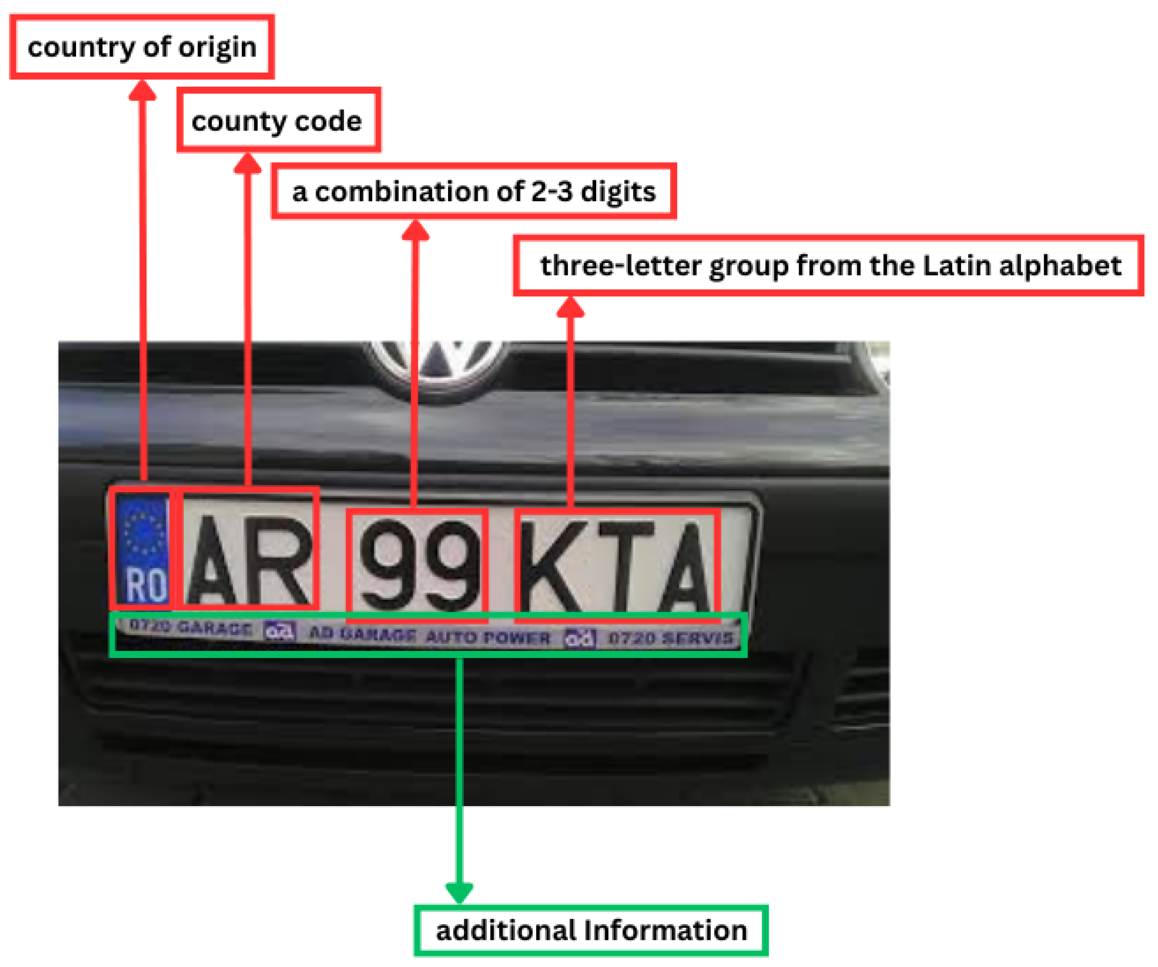
Each vehicle license plate in Romania follows a standardized structure, composed of a county code (consisting of one or two letters), followed by a number of two or three digits and then a sequence of three letters, for example, Figure 2. This combination is unique for each vehicle and allows for its rapid identification. In some cases, the plates may also contain additional information inscribed below the number, such as the name of the car dealership or the location from where the vehicle was purchased, without affecting the validity of the license plate number itself.

3.2. Dataset of Images

The dataset used in this work includes 744 images [21], capturing a total of approximately 500 different vehicles, each having a unique license plate number. The images feature both cars, as well as motorcycles and public transport buses, in order to reflect the variety of means of transportation typically encountered on Romanian roads.

The images were captured from various angles, in natural conditions, to cover a wide range of possible situations in the practical use of the algorithm. The plates shown in the images follow the official Romanian format, including both models issued before 2007 and those compliant with the European standard introduced later.

The dataset was collected and labeled by the authors and was then made publicly available [21], being accessible for reproducing this study or conducting other research for academic purposes. The dataset contains the following types of license plates: Figure 1a,c–e, as these are the most common ones encountered in traffic. It was divided into three subsets: training (80%—594 images), validation (10%—75 images), and testing (10%—75 images), following a standard distribution for machine learning tasks.

3.3. Image Labeling

For labeling the images of the dataset, the platform makesense.ai  [23] was used, a free online tool that allows for manual marking of objects in images. After completing the annotation process, the labels were exported in the format specific to the YOLO network [24], widely used in object detection tasks.

The labeling consisted of manually drawing a bounding box around each license plate present in the image. These boxes mark the exact position of the plate, being essential for the algorithm to learn how to locate them automatically.

The YOLO format [24] assumes a simplified and efficient representation of annotations (see Figure 3), where each line in the label file corresponds to an object (in our case, a license plate), with the following structure:

• class_id—an integer indicating the class of the object (e.g., 0 = license plate);
• X—the position of the center of the box on the X axis, normalized (divided by the width of the image—see Formula (1));
• Y—the position of the center of the box on the Y axis, normalized (divided by the height of the image—see Formula (2));
• width—the width of the box, normalized;
• height—the height of the box, normalized.

The formula for the normalized X coordinate of the bounding box center is given by

$$X={\displaystyle \frac{X_c}{Im{g}_w}}={\displaystyle \frac{X_1+X_2}{2·Im{g}_w}}$$

(1)

The formula for the normalized Y coordinate of the bounding box center is given by

$$Y={\displaystyle \frac{Y_c}{Im{g}_h}}={\displaystyle \frac{Y_1+Y_2}{2·Im{g}_h}}$$

(2)

where

• $X_1,Y_1$ are the coordinates of the top-left corner of the bounding box (in pixels);
• $X_2,Y_2$ are the coordinates of the bottom-right corner of the bounding box (in pixels);
• $X_c,Y_c$ represent the center coordinates of the bounding box, computed as the average of the two corners;
• $Im{g}_w,Im{g}_h$ are the width and height of the image (in pixels).

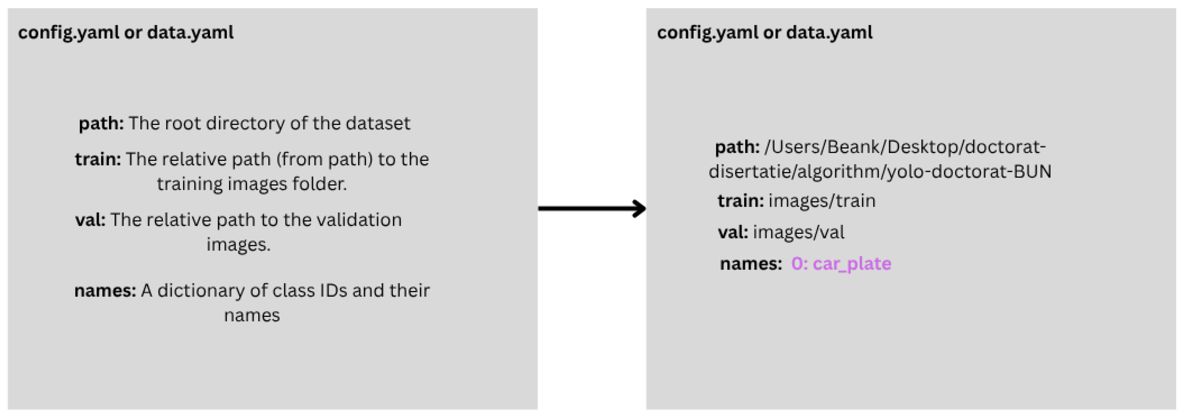
After completing the image labeling process, two main directories were generated: images and labels. Inside the image directory, there are three subdirectories: train, val, and test, each containing the corresponding image sets for training, validation, and testing. The structure is mirrored in the labels directory, which contains the annotation files associated with each image, in YOLO format.

The connection between these resources and the YOLO detection algorithm is made through the config.yaml file (Figure 4), which specifies the paths to the train and val directories, as well as the labeled object class, in this case “car_plate”.

3.4. Model Used

For the license plate detection task, the YOLO model was used, in its most recent available version, YOLOv12 [20,25]. The YOLOv12 model was released on 18 February 2025, marking a new stage in the evolution of object detection architectures.

The YOLOv12 architecture combines feature extraction through CNNs with an advanced attention system, optimized for fast detection tasks. Due to a balanced design between complexity and performance, the model proves efficient in real-time applications, ensuring accurate detection without high computational costs.

Table 1. YOLOv12 models [25]—performance detection comparison.

Model	Resolution (px)	mAP@0.5:0.95	Time (T4)	Params (M)	FLOPs (G)	Comparison (mAP/speed)
YOLO12n	640	40.6	1.64 ms	2.6	6.5	+2.1%/−9% vs. YOLOv10n
YOLO12s	640	48.0	2.61 ms	9.3	21.4	+0.1%/+42% vs. RT-DETRv2
YOLO12m	640	52.5	4.86 ms	20.2	67.5	+1.0%/−3% vs. YOLOv11m
YOLO12l	640	53.7	6.77 ms	26.4	88.9	+0.4%/−8% vs. YOLOv11l
YOLO12x	640	55.2	11.79 ms	59.1	199.0	+0.6%/−4% vs. YOLOv11x

[25] presents the performance results of the different YOLOv12 model variants—nano (n), small (s), medium (m), large (l), and extra-large (x)—evaluated on the COCO val2017 validation set [25]. The following metrics are included: mAP@0.5:0.95, which represents the mean of the Average Precision (AP) values calculated at ten IoU overlap thresholds (from 0.5 to 0.95, in steps of 0.05), inference time, model size, and computational complexity.

To evaluate the performance and technical characteristics of the YOLOv12 variants, a comparative analysis of the main performance metrics is conducted. The following section highlights the relationships between detection accuracy, model complexity, and inference speed across the five model versions (n, s, m, l and x):

• Resolution (px): All models use the same resolution of 640 px.
• mAP@0.5:0.95: YOLO12x has the highest mean Average Precision (mAP), at 55.2%.
• Inference Time (ms): Inference time increases as model complexity increases, from 1.64 ms for YOLO12n up to 11.79 ms for YOLO12x.
• Parameters (M): The number of parameters increases from 2.6 M for YOLO12n to 59.1 M for YOLO12x, indicating higher model complexity.
• FLOPs (B): Computational cost (FLOPs) grows proportionally with model size, from 6.5 B for YOLO12n to 199.0 B for YOLO12x.
• Comparison: YOLOv12 shows improvements in mAP compared to YOLOv10, YOLOv11, and RT-DETRv2, but with some trade-offs in inference speed.

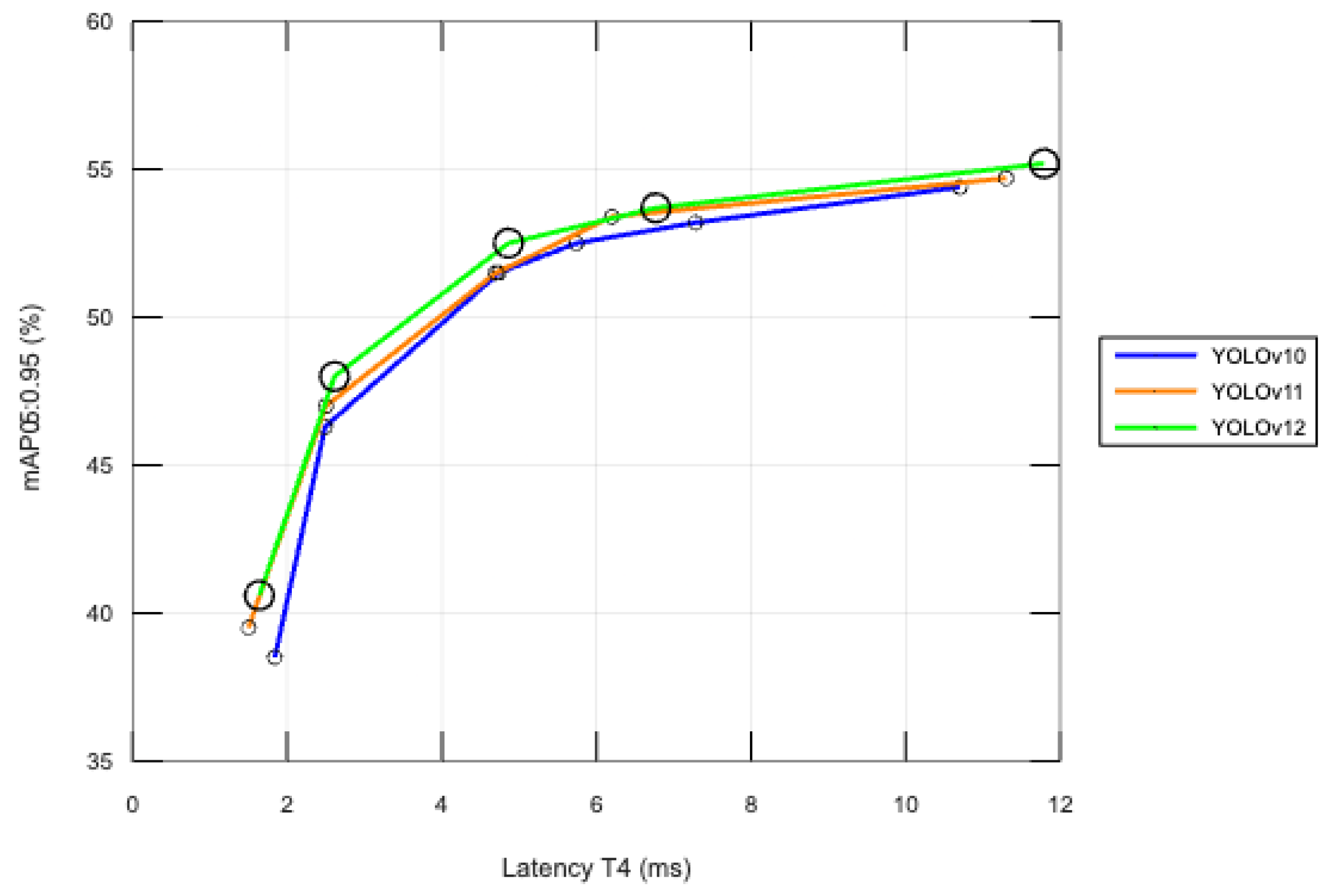
Figure 5 illustrates the performance of three successive versions of the YOLO (You Only Look Once) architecture—YOLOv10, YOLOv11, and YOLOv12—based on inference time (Latency T4, expressed in milliseconds) and mean accuracy (mAP@0.5:0.95), using the COCO validation dataset.

The X axis represents the inference time (latency) on the NVIDIA T4 GPU, while the Y axis shows the mAP@0.5:0.95 score:

• YOLOv10 (blue line): This provides a decent balance between speed and accuracy. Latency ranges from 1.84 ms to 10.7 ms, while mAP@0.5:0.95 increases from 38.5% to 54.4%;
• YOLOv11 (orange line): This brings significant improvements over YOLOv10, with a clear increase in mAP@0.5:0.95 at comparable latency levels. For example, at 4.7 ms, YOLOv11 achieves 51.5% mAP@0.5:0.95 compared to 46.3% for YOLOv10;
• YOLOv12 (green line): This delivers the best results among all analyzed versions. For the same inference time, YOLOv12 attains higher mAP values, indicating greater architectural efficiency. For instance, at 4.86 ms, YOLOv12 reaches 52.5%, approximately +1% above YOLOv11 at the same latency.

In this study, for the task of license plate detection, the YOLOv12s model was chosen. Both YOLOv12n and YOLOv12s models were trained and compared, with the latter achieving superior performance, which is why it was selected for use. Extending training to larger models (such as YOLOv12m, YOLOv12l, or YOLOv12x) was not considered necessary, since the task is specific and focused on a single object type that does not require the complexity of larger models. Furthermore, using a compact model like YOLOv12s offers significant advantages in terms of inference speed and resource consumption. For these reasons, among the five available YOLOv12 variants, YOLOv12s was deemed the most suitable choice for this study. For the vehicle type detection task, the YOLOv12s model pretrained on the COCO dataset was used.

3.5. Implementation Environment

For image annotation, the online platform makesense.ai [23] was used, which allows for object marking directly in the browser and exporting annotations in a YOLO-compatible format.

The model was trained locally using Jupyter Notebook (version 7.3.3) on a 16 inch MacBook Pro with an Apple M3 Pro processor. It features a 12-core CPU and an integrated 18-core GPU, providing good performance for moderate machine learning tasks. Although the architecture used does not support CUDA, PyTorch [26] (the YOLO model from ultralytics is built on PyTorch) was utilized with MPS (Metal Performance Shaders) support, enabling the use of the integrated Apple GPU during training.

The operating system used was macOS Sequoia 15.3.2 (24D81). The development environment was configured as follows:

• JupyterLab for running the code;
• Python 3.11.11;
• Libraries used:

  −

  ultralytics—for working with the YOLO model;

  −

  cv2 (OpenCV)—for image processing;

  −

  numpy—for numerical operations;

  −

  matplotlib—for displaying graphs and images;

  −

  paddleocr—PaddleOCR v2.10.0—for text recognition (OCR).

This setup was sufficient for basic training and local model testing, without the need for external servers or dedicated graphics cards.

4. Detection and Classification Method

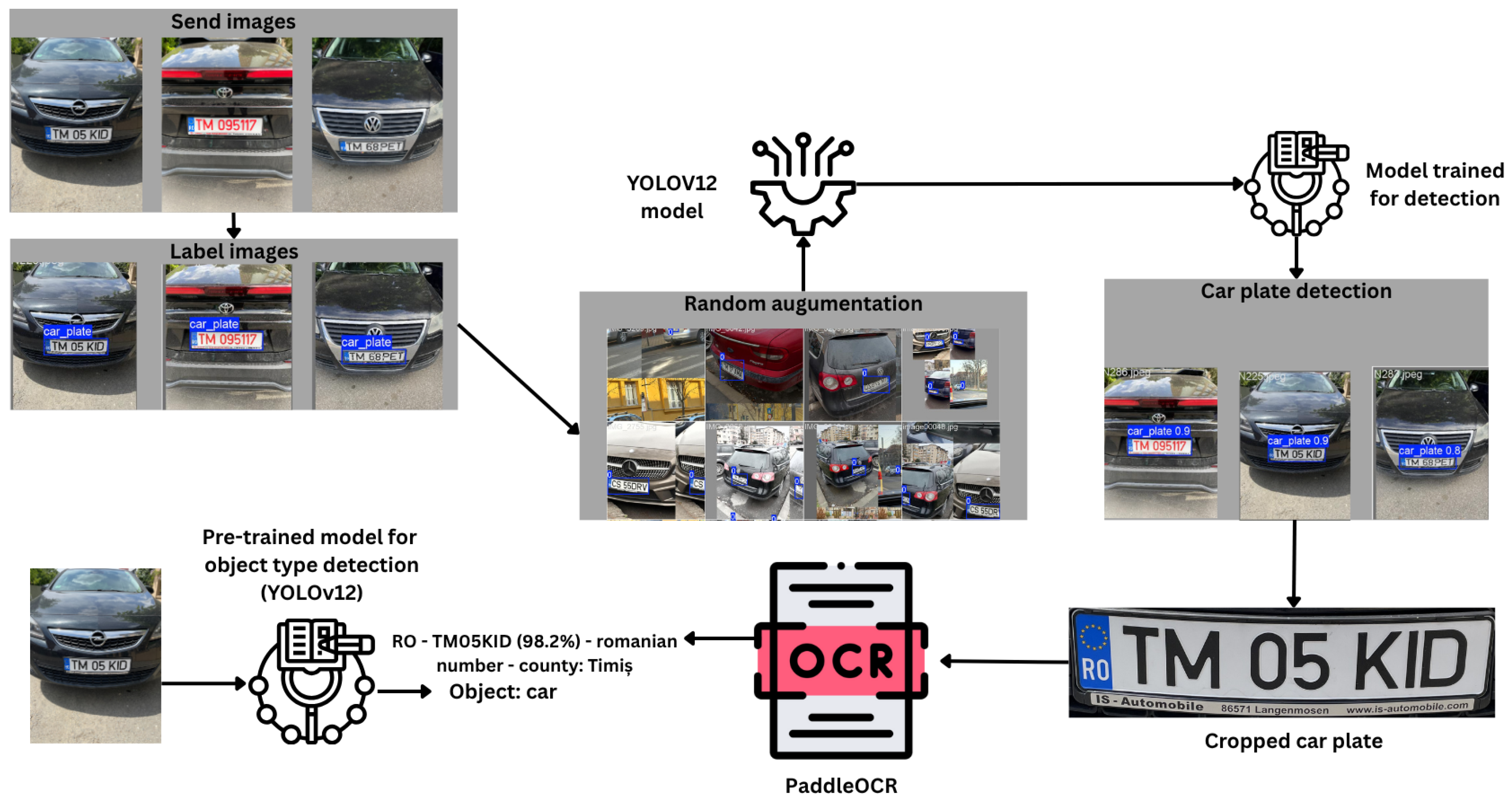
This section presents the method used to extract the license plate number and the vehicle type from images. It begins with a general diagram showing the process leading to license plate detection, text recognition from the plate, and identification of the vehicle type in the image.

Before training the model, a simple algorithm was implemented to check whether each image has a corresponding annotation file and vice versa. This step was important to avoid errors caused by missing or mismatched data.

Next, the steps of data preparation, the choice of training parameters, and the methods used to evaluate the model’s performance are explained, such as precision (Formula (3)), recall (Formula (4)), F1 score (Formula (5)), mAP@0.5 (Formula (6)), mAP@0.5:0.95 (Formula (7)), and the evolution of losses. In the end, the part related to identifying the type of vehicle from the image is presented separately, explaining how it was accomplished and which model was used.

4.1. Overview of the Proposed Method

To provide an overview of how the training and detection process was carried out, this section presents, through Figure 6, the main steps involved: selection and annotation of the dataset, image augmentation, actual training of the YOLOv12 model, performance evaluation, license plate detection, and the identification of the types of vehicles in which they are found.

After detection, the license plates are cropped from the image and processed using the PaddleOCR library [22], which performs text recognition. For each identified text segment (e.g., a word or a sequence of characters), a global confidence score is computed. The text is retained only if this score exceeds the threshold of 0.6. Subsequently, the text is standardized by removing irrelevant symbols and converting it to uppercase. Its validity is then checked using regular expressions that test compliance with Romanian or foreign license plate formats (such as DE, IT, GR, etc.).

In parallel, the same type of YOLOv12 model (pretrained for object detection) is used to identify the type of vehicle in the image. The position of each detected license plate is compared with the previously identified objects in order to determine the type of vehicle it belongs to (e.g., car, truck, motorcycle).

For Romanian license plates, the county of origin is also displayed, while international plates are marked as foreign.

Figure 6 provides a visual summary of the workflow.

4.2. Training YOLOv12 for Vehicle License Plate Detection

As previously presented, the YOLOv12 model was used for training. It is the most recent development in the YOLO series and currently provides the best results (Figure 5).

Table 2. Configuration parameters used for YOLOv12s training.

Parameter	Value	Description
task	detect	Task of the model: object detection
model	yolo12s.pt	Pretrained YOLO model used as a base
data	config.yaml	Dataset configuration (Figure 4)
epochs	20	Total number of training epochs
batch	16	Batch size
imgsz	640	Input image resolution
optimizer	auto	Automatic optimizer selection
pretrained	true	Uses pretrained weights
patience	100	Early stopping if no improvement occurs
val	true	A validation set is used
lr0	0.01	Initial learning rate
mosaic	1.0	Mosaic augmentation enabled
momentum	0.937	Momentum for optimization
auto_augment	randaugment	Automatic augmentation technique
weight_decay	0.0005	L2 regularization penalty

presents the parameters used for training the model. These parameters are essential for the correct configuration and training of the YOLO model, playing a key role in optimizing performance and adapting the learning process to the specific task of license plate detection.

One of the most important parameters used in training the YOLO model is auto_augment, which in this work is set to RandAugment. This value represents a key data augmentation technique that significantly contributes to improving the performance and generalization ability of the detection model.

RandAugment stands out by randomly applying two different transformations to each image in the dataset, with each transformation having a controlled level of intensity. This approach simplifies the augmentation process compared to more complex techniques and significantly helps prevent overfitting, making the model more adaptable to varying environmental conditions.

During the training process, data augmentation techniques such as RandAugment apply random transformations to the images in the training set. These transformations can be seen in files like train_batch0, train_batch1, and other batches generated throughout training (Figure 7). These images reflect the effects of the augmentations applied, which include random rotations, color adjustments, object translations, flips, and other distortions. By analyzing these images, one can observe how augmentations modify the original data, helping the model become more robust and recognize objects (in our case, license plates) under a wider range of visual conditions. The original images are stored and used during training, but the augmented images are generated on-the-fly and not saved, which keeps storage requirements low while increasing data variability. Although the initial dataset contains only 744 images, the use of RandAugment during training results in multiple variations of each image being seen at every epoch. During the 20 training epochs considered, the model is exposed to approximately 14,880 virtual samples (images), which effectively enhances the training process by incorporating uncertainty factors such as camera angle, visibility conditions, and lighting variations.

Examples of augmentation types that can be observed in Figure 7 include the following:

• Flips (horizontal/vertical): the image and bounding boxes are flipped;
• Scaling (random resizing): enlarging or shrinking objects;
• Random Crop: randomly cutting a part of the image;
• Rotation: small rotations, useful in scenarios with varied orientations;
• Brightness/Contrast Adjustment: changes in brightness and contrast;
• Mosaic Augmentation: combines four images into one (very effective);
• MixUp: combining two images by partial overlay;
• CutOut: masking random regions of the image, etc.

The outer images, from which the arrows originate, represent the original input images. The images pointed to by the arrows are the augmented versions generated from those originals. Various data augmentation techniques were applied to create these variants, such as brightness adjustments (either increasing or decreasing brightness), horizontal flipping, zooming (in or out), and others. The central images are already augmented; however, they were not displayed alongside the original ones to keep the figure uncluttered.

4.3. Evaluation Metrics

To understand and quantify the performance of an object detection model like YOLOv12, it is essential to use a standardized set of metrics that reflect how well the model detects and classifies objects present in an image. In this project, the YOLOv12 model was trained exclusively for license plate detection, while vehicle type detection was performed using the YOLOv12 model pretrained on the COCO dataset. The extraction of the license plate number was carried out using the PaddleOCR library.

The most relevant metrics used in this context are presented below. These metrics are calculated after each training epoch and are useful both for tracking performance progress over time and for identifying potential issues such as overfitting or class imbalance.

Precision [27]—out of all the license plates “detected” by the model, this represents how many are actually correct.

The formula for precision is given by

$$\mathrm{Precision}={\displaystyle \frac{TP}{TP+FP}}$$

(3)

where

• $TP$ is the number of True Positives—license plates correctly detected by the model (predictions that sufficiently overlap with a ground-truth plate, typically with an Intersection over Union (IoU) threshold of at least 0.5);
• $FP$ is the number of False Positives—predictions made by the model that do not correspond to any actual license plate (insufficient overlap or non-existent object).

Recall (True Positive Rate or TPR) [27]—out of all the license plates that actually exist in the image, this represents how many were correctly found by the model.

The formula for recall is given by

$$\mathrm{Recall}={\displaystyle \frac{TP}{TP+FN}}$$

(4)

where

• $TP$ is the number of True Positives, as defined above;
• $FN$ is the number of False Negatives, meaning the real license plates present in the image that the model failed to detect (i.e., there is no prediction with sufficient overlap for those plates).

F1 score [28]—the harmonic mean of precision and recall; it provides a balanced evaluation, especially when there is an imbalance between the number of detected license plates and the actual ones.

The formula for F1 score is given by

$$\mathrm{F}1\mathrm{Score}=2·{\displaystyle \frac{\mathrm{Precision}·\mathrm{Recall}}{\mathrm{Precision}+\mathrm{Recall}}}$$

(5)

mAP—mean Average Precision [29]—mAP represents the average of the Average Precision (AP) values across all classes. In the context of YOLO, the following are commonly used:

• mAP@0.5 [29]—IoU threshold of 0.5, indicating correct detections when the overlap between the model’s prediction and the actual license plate is at least 50%.
• mAP@0.5:0.95 [29]—average across IoU thresholds from 0.5 to 0.95, with a step size of 0.05; this is typically used as the standard in the COCO benchmark.

The formula for mAP@0.5 is given by

$$\mathrm{mAP}@0.5={\displaystyle \frac{1}{C}}\sum _{c=1}^C{\mathrm{AP}}_c^{\mathrm{IoU}=0.5}$$

(6)

where

• C is the total number of classes (in this work, $C=1$, since only the license plate class is being detected);
• ${\mathrm{AP}}_c^{\mathrm{IoU}=0.5}$ is the Average Precision for class c, computed at an IoU threshold of 0.5 (i.e., a prediction is considered correct if it overlaps with the ground truth by at least 50%).

The formula for mAP@0.5:0.95 is given by

$$\mathrm{mAP}@0.5:0.95={\displaystyle \frac{1}{10C}}\sum _{c=1}^C\sum _{k=0}^9{\mathrm{AP}}_c^{\mathrm{IoU}=0.5+0.05k}$$

(7)

where

• 10 IoU thresholds are used (ranging from 0.5 to 0.95, in steps of 0.05), and the AP is calculated for each threshold;
• ${\mathrm{AP}}_c^{\mathrm{IoU}=x}$ is the Average Precision for class c at the IoU threshold x.

Loss Evolution—box_loss, cls_loss, dfl_loss (for both train and val):

• Box Loss: This measures the error in localizing the license plates (predicting the bounding box coordinates for each plate). A low loss indicates that the model accurately localizes the license plates, with precise predictions of their positions in the image.
• Cls Loss: This measures the classification error of the license plates (correctness in identifying the object class). A low loss indicates that the model correctly classifies the license plates without confusing them with other objects in the image.
• DFL Loss: This loss is used to improve the model’s performance on difficult instances (license plates that are hard to detect due to particular conditions such as angles, lighting, or poor image quality). A low loss suggests that the model successfully identifies these more challenging instances.

4.4. Vehicle Type Detection

In addition to license plate detection, the detection of the object containing the license plate was also implemented. This detection was performed using the pretrained YOLOv12 model for this task. Identifying the object surrounding the license plate is important for verifying the authenticity of the image and for detecting intrusion attempts, such as cases where a person is holding a license plate in their hand or situations where only certain categories of vehicles (e.g., based on weight) are permitted to pass.

To detect objects that may have license plates, a standard list of classes from the COCO dataset was used. However, within the application, only categories corresponding to vehicles that typically carry license plates are relevant, such as car, motorcycle, bus, and truck.

The original COCO list contains many more object categories, but for this project only those directly related to the intended purpose were retained. Of course, the selection can be easily adapted if new requirements arise or if a different dataset is used.

It is important to emphasize that, for this stage, the object containing the previously detected license plate was selected directly, thereby avoiding processing other irrelevant objects in the image and reducing execution time.

After the license plate is localized in the image, it is checked whether it lies within a previously detected object. If the license plate is fully contained within the boundary of such an object, that object is considered to represent the vehicle to which the plate is attached.

The object type is determined based on the category assigned by the model, and this information is included in the final output displayed alongside the recognized license plate number. This ensures that only relevant objects (those actually containing a license plate) are considered, thereby optimizing both the accuracy and performance of the algorithm.

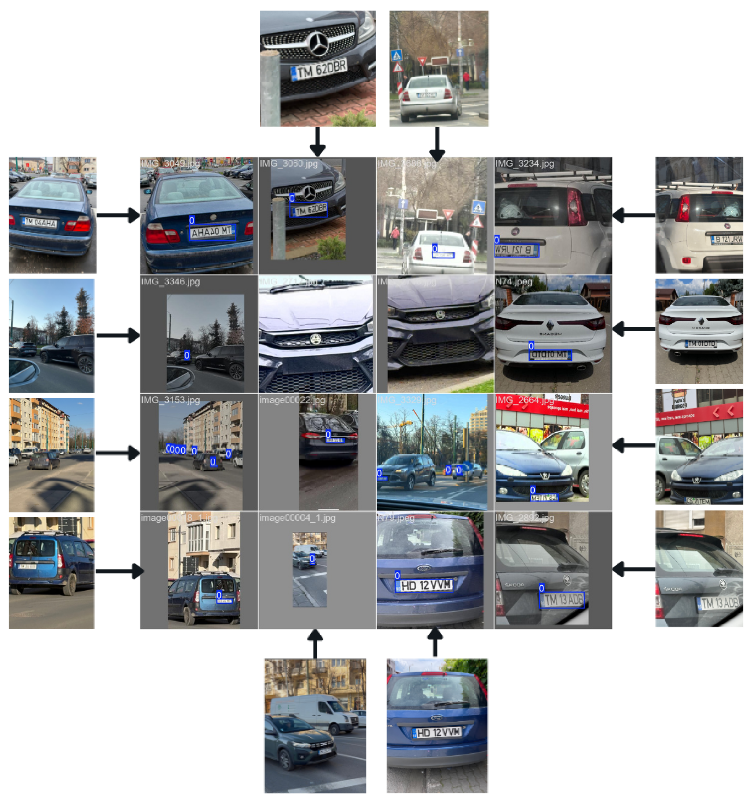
The final result is displayed on the Figure 8: each license plate is highlighted with a colored bounding box (green for Romanian plates, red for foreign plates), and next to it appears the recognized text, confidence score, and the detected vehicle type. Thus, the system not only automatically extracts the license plate numbers but also associates them with the correct visual context—that is, the vehicle to which they belong.

5. Results and Validation

This section provides a detailed analysis of the performance of the YOLOv12 model, which was trained for license plate localization in images. The evaluation was conducted using the metrics defined in Section 4.3, focusing on the model’s performance during different stages of the training process.

The section is divided into three subsections: the first subsection details the model’s performance during training, with a focus on the last five epochs evaluated on the validation set, highlighting the evolution of the metrics and the point of convergence; the second subsection analyzes the model’s behavior after training has been completed, using the precision–recall curve, P_curve, R_curve, F1_curve, and the Loss Over Epochs graphs, and it includes the final evaluation on the test set, which reflects the model’s generalization capability under conditions not seen during training; the third subsection provides a summary comparison between the latest version of the YOLO model, YOLOv12, and the previous version, YOLOv11.

5.1. Analysis of Model Progress and Performance During Training

Following the training of the YOLOv12 model, a file named results.csv is generated, which contains the results obtained for each epoch based on the metrics defined in Section 4.3. These results are computed using the validation set specified in the configuration file and reflect the model’s performance on data not seen during training but used for evaluation throughout the learning process.

The results obtained during the last 5 epochs, out of the 20 total training epochs, are presented in

Table 3. Evaluation metrics on the validation set during the last 5 epochs of YOLOv12 training.

Epoch	Time	box_loss	cls_loss	dfl_loss	Precision	Recall	F1	mAP@0.5	mAP@0.5:0.95
16	8861.030	1.049	0.616	0.992	0.988	0.950	0.969	0.975	0.701
17	9428.170	1.006	0.598	0.971	1.000	0.951	0.975	0.973	0.720
18	9996.460	0.985	0.589	0.960	0.984	0.952	0.968	0.972	0.726
19	10,530.200	0.988	0.564	0.956	1.000	0.952	0.975	0.979	0.739
20	11,068.000	0.903	0.534	0.937	0.998	0.940	0.968	0.981	0.737

.

As observed, the model maintained very strong performance throughout the last five training epochs. The values for precision, recall, and the calculated F1 score were high, indicating accurate and efficient detection. Moreover, the mAP@0.5 remained high, while mAP@0.5:0.95 progressively increased, reflecting an increasingly better generalization capability under varied conditions.

In parallel, the loss values on the validation set (box_loss, cls_loss, and dfl_loss, represented in the lower graphs of Figure 9 by the blue, green, and red curves, respectively) showed a slight decrease, indicating ongoing refinement and a reduction in localization and classification errors. In the final epoch (epoch 20), relatively low loss values were recorded confirming stable model convergence. The best generalization results were achieved in epoch 19, which yielded the highest mAP@0.5:0.95 score.

Training was not extended beyond 20 epochs because the model had reached a point where its performance had stabilized, and subsequent epochs did not yield significant improvements. The learning rate had also decreased considerably by epoch 20 (0.000119), indicating that the model was approaching convergence.

Throughout the YOLOv12 training process, the model’s performance is continuously monitored after each epoch, and the system automatically retains the checkpoint corresponding to the best validation performance. As a result, the most optimal version of the model is available at the end of training and can be directly used for detection tasks. This approach ensures an optimal selection of trained parameters, helping to prevent overfitting and maximize accuracy in real-world application scenarios.

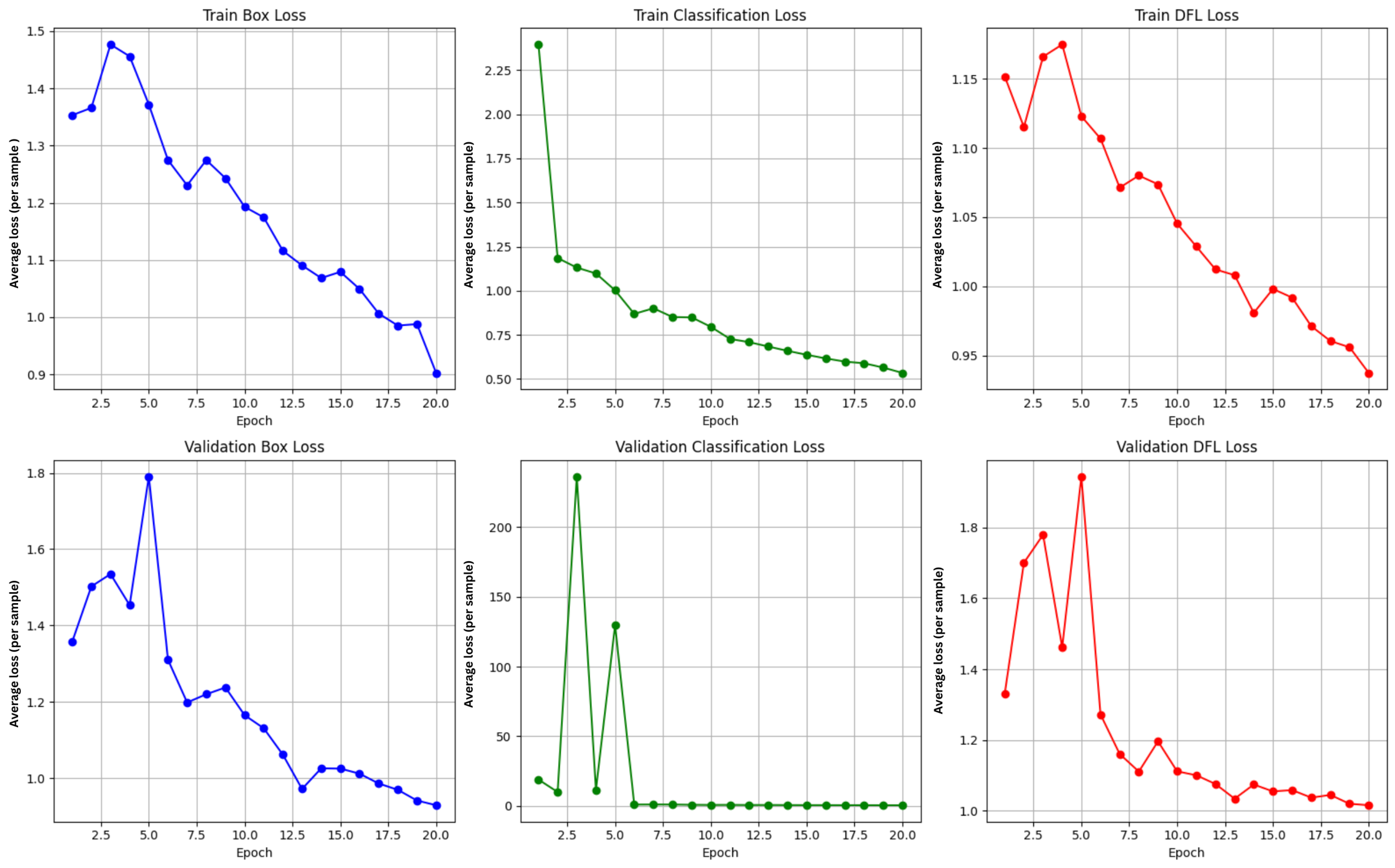
Over the course of the 20 training epochs (Figure 9), the YOLOv12s model exhibited a clear positive trend, reflected both in the reduction in loss values and in the overall improvement in performance.

The box_loss decreased from 1.353 to 0.903 on the training set and from 1.357 to 0.930 on the validation set, indicating increasingly accurate localization of license plates (blue line in Figure 9). In parallel, the cls_loss showed a significant reduction from 2.396 to 0.534 (train) and from 18.901 to 0.468 (val), clearly reflecting improved classification of the detected objects (green line in Figure 9). Additionally, the dfl_loss (Distribution Focal Loss), which contributes to the precision of bounding box position prediction, dropped from 1.151 to 0.937 (train) and from 1.331 to 1.015 (val), confirming increasingly accurate object positioning (red line in Figure 9).

These trends support the conclusion that the model learned effectively throughout training, gradually optimizing its detection and classification capabilities for vehicle license plates under varied conditions.

To clarify the nature of the loss values, the Y axis was labeled as “Average loss (per sample).” Since loss measures prediction error, lower values are better, and an ideal model would achieve a loss of 0. It should be noted that loss does not have a physical unit of measurement.

5.2. Analysis of Trained Model’s Performance

In addition to the CSV file generated during training, several plots are also created after training is completed. These plots are computed on the validation set and serve to highlight optimal performance points, providing a detailed view of the model’s final behavior and its generalization capacity.

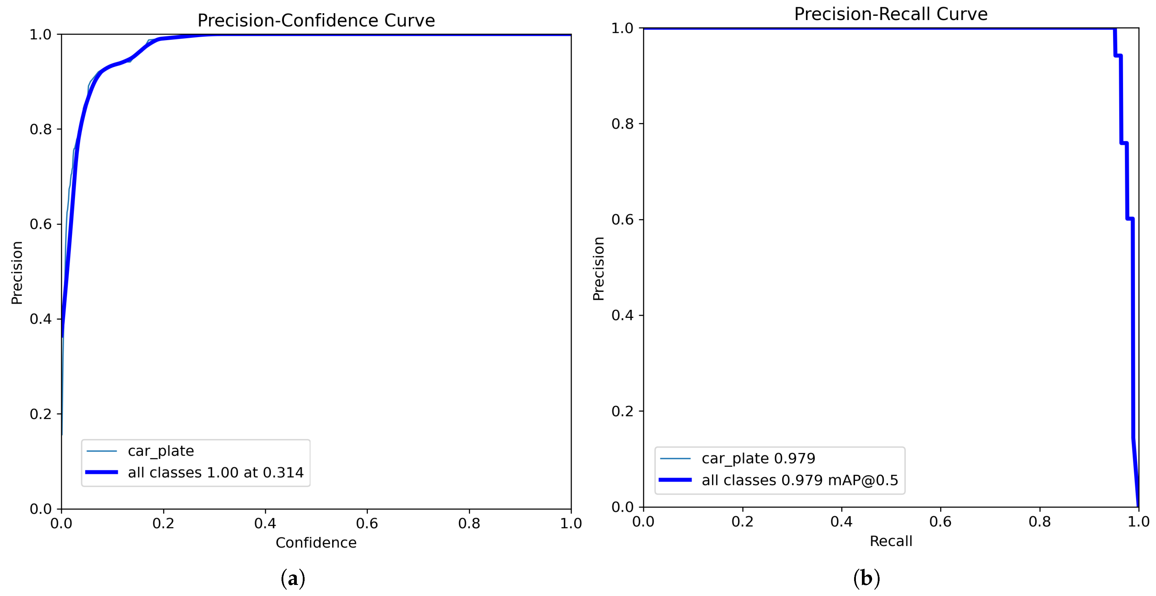
By analyzing the precision–confidence curve [29], shown in plot (a) of Figure 10, it can be observed that if only predictions with a confidence score above 0.314 are kept, the model will return only correct results for license plates. The plot displays two lines: one for the “car_plate” class and a global average, which is automatically shown even in single-class scenarios.

This confidence threshold (0.314) represents a safety margin for the model: the closer a prediction’s score is to 1, the more confident the model is in having correctly detected a license plate. By setting this threshold, uncertain predictions are filtered out, reducing the risk of errors. Thus, setting a threshold of 0.314 (or higher) ensures that only high-confidence predictions are retained.

For applications where errors are unacceptable (such as issuing fines or automated access control), a confidence threshold of 0.314 or higher is recommended. If the goal is to detect as many license plates as possible, even at the risk of occasional errors, a lower threshold, such as 0.2, may be used.

As shown in part (b) of Figure 10, the precision–recall curve [29] indicates that the model provides highly accurate results (precision of 0.979) up to a recall of approximately 0.95. Beyond this point, precision becomes unstable and drops sharply to very low values (below 0.1), especially at high recall levels. This behavior suggests that, in an attempt to maximize recall, the model generates a large number of false positive predictions, thus significantly compromising precision.

Plot (a) in Figure 11 shows that the model maintains a high recall, above 0.95, for confidence score values between 0 and 0.6. Beyond this threshold, recall decreases rapidly and reaches zero before the confidence score hits 0.9, remaining at zero up to 1. This trend suggests that although the model performs well at moderate confidence levels, filtering predictions with scores above 0.6 results in the loss of many detections. Therefore, it is recommended to choose a confidence threshold within the 0.2–0.6 range to maintain an optimal balance between precision and recall.

The F1 curve [29], shown in plot (b) of Figure 11, indicates that the F1 score starts at approximately 0.25 for low confidence thresholds (near 0.0) and quickly rises to nearly 0.98 for confidence values between 0.0 and 0.2. This high score remains stable up to around the 0.6 threshold, suggesting a good balance between precision and recall (see Formula (5)). Beyond 0.6, the score drops sharply, reaching 0 near the 0.9 mark and staying at zero up to 1. Therefore, confidence thresholds between 0.2 and 0.6 are recommended to maintain optimal model performance and avoid significant detection losses.

For model evaluation, an additional analysis was conducted on the test set using the val function with different parameters for conf (confidence threshold) and IoU = 0.5 (the IoU threshold for correct detections) (see

Table 4. Evaluation results of the model on the test set.

Conf	IoU	Precision	Recall	F1 Score	mAP@0.5	mAP@0.5:0.95
0.30	0.50	0.996	0.961	0.978	0.980	0.774
0.50	0.50	0.996	0.961	0.978	0.980	0.776
0.70	0.50	1.000	0.792	0.884	0.896	0.730

Metrics are computed on the test set using the specified confidence and IoU thresholds.

). This process generated relevant metrics such as precision, recall, F1 score, and mAP at both IoU 0.5 and 0.5–0.95.

The evaluation of the model across different confidence thresholds (0.3, 0.5, and 0.7) demonstrated stable and accurate performance at lower thresholds. At both 0.3 and 0.5, the model achieved identical precision and recall values, along with high F1 scores, mAP@0.5, and mAP@0.5:0.95 metrics. These consistent results confirm the model’s robustness within the moderate confidence range.

At a stricter threshold of 0.7, the precision reached the maximum value, but the recall dropped significantly, leading to a decrease in the F1 score and lower mAP values. This trend highlights the trade-off between detection strictness and coverage rate, indicating that an overly high threshold may negatively impact the overall detection effectiveness.

5.3. YOLOv12 vs. YOLOv11: Performance Evaluation on the Proposed Dataset

To analyze the performance improvement from the previous version (YOLOv11) to the latest one (YOLOv12), a YOLOv11 model was also trained. The performance comparison between the two versions was carried out based on the results obtained during the final training epoch (epoch 20) (see

Table 5. Performance comparison between YOLOv11 and YOLOv12 models at the final training epoch.

Model	Epoch	Precision	Recall	F1 Score	mAP@0.5	mAP@0.5:0.95
YOLOv11	20	0.998	0.929	0.962	0.973	0.753
YOLOv12	20	0.998	0.940	0.968	0.981	0.737

Values are taken from the final training epoch (epoch 20) for both models, evaluated on the validation set.

), as well as through evaluation on the test set (see

Table 6. Comparison of YOLOv12 and YOLOv11 model performance on the test set at a confidence threshold of 0.5 and IoU of 0.5.

Model	Precision	Recall	F1 Score	mAP@0.5	mAP@0.5:0.95
YOLOv11	0.974	0.961	0.967	0.979	0.769
YOLOv12	0.996	0.961	0.978	0.980	0.776

Evaluation performed at a confidence threshold of 0.5 and an IoU threshold of 0.5.

). This approach ensures an objective and relevant comparison under real-world conditions.

Comparing the final training epoch of the two models, YOLOv12 demonstrated better overall performance than YOLOv11. Both models achieved very high precision, but YOLOv12 showed a higher recall and a better F1 score, indicating a more balanced detection capability. Additionally, YOLOv12 attained a higher mAP@0.5. Although YOLOv11 had a slight edge in mAP@0.5:0.95, YOLOv12 proved to be more stable and efficient overall.

The final evaluation on the test set confirms that YOLOv12 achieved superior performance compared to YOLOv11 for the analyzed task. YOLOv12 outperformed YOLOv11 in four out of five evaluation metrics (precision, F1 score, mAP@0.5, and mAP@0.5:0.95), while matching it in recall. Notably, YOLOv12 achieved a 2.3% increase in precision (from 97.4% to 99.6%) and a 1.1% improvement in F1 score (from 96.7% to 97.8%), demonstrating a reduction in false positive detections. Both YOLOv11 and YOLOv12 were trained and evaluated using the same proprietary dataset of 744 primary images, with on-the-fly augmentation during training resulting in approximately 14880 virtual samples (virtual images) over 20 considered training epochs.

Both models exhibited the same recall, indicating a similar capability to detect all relevant objects in the images.

The F1 score, which balances precision and recall, was 0.978 for YOLOv12s compared to 0.967 for YOLOv11s, confirming an advantage of the newer version.

YOLOv12s also had a higher mAP@0.5 and a better mAP@0.5:0.95, indicating improved localization accuracy.

In conclusion, YOLOv12 offers higher accuracy and more reliable detection than YOLOv11, making it more suitable for applications where minimizing classification errors is critical.

5.4. Performance Summary

The results confirm the performance of the proposed model, which, in the final training epoch, achieved a precision of 0.998, a recall of 0.940, an F1 score of 0.968, an mAP@0.5 of 0.981, and an mAP@0.5:0.95 of 0.737 on the validation set, with minimal loss indicators of stable and efficient convergence.

To validate its performance beyond the training data, the model was tested on a dedicated test set. The analysis of these results revealed an optimal confidence threshold of 0.5, at which the model achieved a precision of 0.996, a recall of 0.961, an F1 score of 0.978, and a peak mAP@0.5:0.95 of 0.776. These values confirm the model’s strong generalization capability under diverse, real-world conditions.

Moreover, the model maintains a solid balance between precision and recall within a representative confidence threshold range of 0.3 to 0.5, making it easily adaptable to various application requirements, from maximum detection coverage to high operational reliability.

Overall, YOLOv12 demonstrated better performance than YOLOv11 on the issue analyzed in this study.

6. Conclusions

In recent years, there has been a growing interest in implementing ALPR using modern deep learning techniques. As a result, many recent studies have applied deep learning approaches based on datasets containing vehicles registered in various countries (Germany, Egypt, Israel, Bulgaria, etc.). Summaries of selected studies were presented in the Related Work Section. The YOLO algorithm is part of deep learning, uses CNN as a foundation, and is optimized for speed and accuracy in object detection within images. The YOLO algorithm has become a reference standard in object detection. Recently, many versions of the YOLO algorithm have been successfully used in ALPR.

In the present work, a YOLOv12 model was trained and evaluated for license plate detection in images. The proposed model demonstrated solid performance both during training and in the testing phase, highlighting stable convergence and a good capacity to adapt to various real-world conditions. Evaluation on external data confirmed its potential for generalization and applicability in diverse practical scenarios. Additionally, the model succeeds in maintaining an effective balance between precision and recall across a range of confidence thresholds, being easy to calibrate according to the specific requirements of the application, from complete identification of objects of interest to minimizing false detections.

The main contributions of this research include the construction of a manually labeled dataset, which contains 744 images of vehicles registered in Romania (expanded by augmentation in the training stage to 14,880 images), publicly available on GitHub [21]. Additionally, the source code used for training and evaluation has also been made available to facilitate reuse, verification, and further development by the research community. Also, the proposed system was trained and evaluated for automatic license plate detection in images, using the most recent YOLOv12 model. To the best of the authors’ current knowledge, this is the first documented application of the YOLOv12 version for this problem, the obtained results demonstrating superior performance compared to the previous version. Furthermore, the combination of YOLOv12 and PaddleOCR is, as far as we know, unique among the reviewed studies.

The novelty element of the research consists in the simultaneous integration of three components: (1) the localization of the license plate in the image, (2) the extraction of the text from it, including the identification of the registration county, specific to Romanian license plates, and (3) the identification of the type of vehicle on which it is mounted. This integrated approach considerably extends the applicability area of ALPR systems, which are usually limited to license plate localization and text extraction. The proposed solution can be used to solve problems such as restricting access of certain types of vehicles to specific areas, monitoring traffic flow based on county, or implementing differentiated policies, such as access or parking charges depending on the type of vehicle or its provenance.

A future research direction is the optimization of the proposed system for real-time operation on edge devices, such as smart cameras or embedded units, where local processing can help reduce latency and bandwidth consumption while maintaining high detection accuracy.