Highway Travel-Time Forecasting with Greenshields Model-Based Cascaded Fuzzy Logic Systems

Abstract

Intelligent Transportation Systems (ITSs) play a vital role in improving urban and regional mobility by reducing traffic congestion and enhancing trip planning. A key element of ITS is travel-time prediction, which supports informed decisions for both travelers and traffic management. While non-parametric models offer flexibility, they often require large datasets and significant computation. Parametric models, though easier to fit and interpret, are less adaptable. Fuzzy logic models, by contrast, provide robustness and scalability, adjusting to new data and changing conditions. This paper proposes a cascaded fuzzy logic system for highway travel-time prediction, using the Greenshields model as its reasoning foundation. The system consists of multiple fuzzy subsystems, each representing a highway segment. These subsystems transform traffic flow and density inputs into speed predictions through fuzzification, Greenshields-based rules, and defuzzification. The approach enables localized and segment-specific predictions, enhancing route planning and congestion avoidance. The system’s accuracy is evaluated by comparing its predictions with those of a regression model using real traffic data from the Sun Yat-Sen Highway in Taiwan. Simulation results confirm that the proposed model achieves reliable, adaptable travel-time forecasts, including for long-distance trips.

1. Introduction

An increased traffic flow on highways inevitably leads to longer periods of congestion and a higher risk of accidents. A greater vehicle volume creates bottlenecks and worsens existing congestion, particularly on multi-lane roads where accident rates tend to rise as traffic increases. According to statistics from the Freeway Bureau of Taiwan [1], daily vehicle usage on Taiwan’s highways surpassed 90 million vehicle kilometers (MVKs) in 2024, representing a 3.4% increase compared to the previous year. Traffic congestion between cities has become a major concern for drivers and commuters, driven by rapid population growth and accelerated urbanization in modern cities. Addressing challenges related to highway development, transportation efficiency, congestion, road safety, and environmental pollution requires careful planning and innovative solutions. Intelligent Transportation Systems (ITSs), which integrate vehicles, roadside equipment, and traffic data centers, enable the incorporation of advanced technologies—such as artificial intelligence (AI), the Internet of Things (IoT), and computer networking—into transportation infrastructure and vehicles. These systems collect, analyze, process, and distribute traffic data to support better traffic management, route planning, and safety measures [2,3,4,5]. Intelligence-powered technologies and management strategies within ITS enhance road safety, improve traffic efficiency, and reduce environmental impact by enabling smarter route planning, optimizing traffic signal timings, and supporting autonomous driving. To fully realize the benefits of these technologies, accurate prediction of key traffic parameters is essential. Among these, reliable travel-time predictions play a critical role in ensuring timely arrivals, minimizing congestion, and improving the overall travel costs. Precise travel-time forecasts not only help drivers make informed route choices but also support traffic management efforts to reduce highway congestion [6,7,8].

For individual drivers, vehicle speed is the most convenient parameter for estimating travel time, as it can be predicted for different highway segments based on various traffic data collected from detection devices. Information related to vehicle speed enables ITS to provide drivers with real-time route guidance, helping them avoid congestion and optimize travel time. Traffic prediction schemes can be developed using either parametric or non-parametric modeling approaches [9,10]. A traffic model based on highway data relies on both historical and real-time information to predict and manage traffic flow. The Greenshields, Greenberg, Underwood, and other nonlinear models are widely employed for predicting traffic conditions and supporting traffic management and control on highways [11,12,13,14,15,16]. These models consider vehicle speed, traffic flow, and vehicle density as the key parameters influencing highway traffic dynamics. The Greenshields model establishes a fundamental relationship among speed, flow, and density, offering a foundational understanding of traffic behavior. The Greenberg and Underwood models, as nonlinear extensions of Greenshields’ work, are designed to capture more complex and specialized traffic flow patterns [12,13,17]. These models offer valuable insights into the interactions among vehicle speed, flow, and density, supporting the development of intelligent traffic management systems. Other common parametric models for vehicle speed prediction and travel-time estimation employ statistical or regression analysis techniques. By capturing key characteristics of traffic conditions within a defined problem scope, these models can predict vehicle speed or other traffic status parameters through simulations or computations based on collected data [18,19,20]. In certain scenarios, hybrid algorithms that incorporate the autoregressive integrated moving average (ARIMA) time-series model have demonstrated a superior prediction performance [21,22,23]. The extended Kalman filter (EKF) has also been applied in second-order traffic flow models to enhance traffic status estimation using only fixed sensors. In [24,25], three mixed estimation methods are compared, respectively, to highlight their respective strengths. A traffic optimization decision system in [26] demonstrated iterative updating of model parameters to improve predictions. However, many existing highway travel-time prediction methods still rely heavily on historical data and static models, which often struggle to maintain accuracy when traffic flow conditions change significantly.

Non-parametric models for travel-time prediction typically involve various machine learning techniques and neural network models [10]. These models often require longer training times due to the large volumes of data they process. Many machine learning approaches for travel-time prediction are relatively straightforward—for example, using support vector regression (SVR) for travel-time estimation [27]. A method that enhances travel-time prediction through linear regression is demonstrated in [28]. A genetic algorithm (GA)-based scheme for predicting travel-time intervals is introduced in [29], while a hybrid model combining GA and SVM is proposed in [30] to improve bus arrival time accuracy. Based on large datasets, a dynamic K-nearest neighbors (K-NN) model is presented in [31] to enhance travel-time prediction accuracy. In [32], the K-NN method is integrated with clustering and principal component analysis to create a framework for bus arrival time prediction. Neural networks have also been applied in various contexts. For short-term travel-time prediction on interurban highways [33]. A graph neural network estimator using Google Maps data and meta-gradient-based training schedules is proposed for travel-time prediction in [34]. In addition, time-series linear regression has been combined with eXtreme Gradient Boosting (XGBoost), and Gated Recurrent Unit (GRU) neural networks have been used to develop several high-performance vehicle travel-time prediction methods [4,35]. A neural network incorporating a fuzzy logic scheme for travel-speed prediction is presented in [36].

Fuzzy logic is a valuable approach for situations where information is imprecise and the relationships among various factors are complex. In fuzzy logic systems, rules based on expert knowledge are used to define connections between these factors. As a result, fuzzy logic is well-suited for systems where precise mathematical modeling is difficult or impractical. Its ability to manage uncertainty and vagueness makes it particularly effective for capturing the complexities of traffic flow in ITS [37]. In general, fuzzy logic systems offer advantages over traditional traffic modeling methods, often providing more accurate and robust predictions. Several fuzzy logic systems based on traffic models have been proposed for assessing traffic congestion levels [38,39]. In [40], a fuzzy logic scheme combined with an SVM-based model is used for real-time traffic congestion prediction on road segments. For rating traffic congestion levels, a machine learning method integrated with a fuzzy comprehensive evaluation scheme (MF-TCPV) is presented in [5]. Additionally, a fuzzy inference system is developed in [41] to select appropriate modes for a dynamic and intelligent traffic light control system based on real-time traffic information.

Traffic conditions are inherently unpredictable and influenced by many dynamic factors. Fuzzy logic provides an effective approach to incorporating expert knowledge and experience into traffic models while reducing modeling complexity. This leads to more realistic and effective predictions. Both fuzzy logic and neural networks are widely utilized in modern ITS for tasks such as pattern recognition, classification, and predictive modeling. The selection between these approaches depends on the complexity of the problem, the nature and availability of data, and the need for interpretability. Neural networks, particularly deep learning models, consist of multiple layers of interconnected artificial neurons that simulate aspects of human cognitive processing. These models learn from large datasets through optimization algorithms such as backpropagation and gradient descent. They are highly effective for capturing nonlinear relationships in complex data and have shown an exceptional performance in real-time traffic prediction, incident detection, and vehicle behavior analysis. However, neural networks often require extensive labeled data and high computational power and are often limited in interpretability. In contrast, fuzzy logic provides a rule-based, transparent, and human-readable framework for handling uncertainty and imprecision in data. It employs linguistic variables and incorporates expert knowledge through if-then rules, making it especially suitable for systems that are difficult to model mathematically. Fuzzy logic is particularly advantageous in ITS applications where explainability and system transparency are critical. A fuzzy logic-based model is generally easier to implement and maintain than traditional mathematical models. This paper proposes a highway travel-time prediction method based on cascaded fuzzy logic systems. In the proposed approach, each subsystem corresponds to a specific highway segment and is developed using the Greenshields model for short-range vehicle speed prediction. Two input parameters—traffic flow and density—are used in the fuzzy rules to determine the output variable, vehicle speed, which serves as the basis for evaluating the travel time. Fuzzy rules derived from Greenshields theory define the relationships between these inputs and outputs. During defuzzification, the outputs from activated rules are combined and converted into a single crisp value representing the predicted speed or travel time. Since a highway route typically consists of multiple segments, the proposed system establishes a Greenshields-model-based fuzzy logic subsystem for each segment, allowing it to dynamically adapt to real-time conditions segment by segment. The vehicle speed for each segment can thus be predicted in advance, enabling the estimation of the required travel time. Each fuzzy logic subsystem predicts the travel time for its corresponding segment and passes the result to the next subsystem. By cascading these subsystems sequentially along a route, the total travel time for the entire highway route can be calculated. The experimental evaluation compares the performance of the proposed fuzzy logic system with regression models using data collected from roadside sensors. This comparison highlights the advantages of the cascaded fuzzy logic system, particularly its ability to handle long-range highway routes and provide a more practical solution for travel-time prediction. Our main contributions are summarized as follows:

• We propose a cascaded fuzzy logic system for predicting travel times along planned highway routes. The system consists of multiple fuzzy logic subsystems, each built on the Greenshields model to predict the vehicle speed for a specific road segment. The predicted vehicle speed from each subsystem is dynamically updated based on current traffic conditions on that segment. By cascading these subsystems sequentially—one for each designated segment—and summing the predicted travel times, the total travel time for the entire route can be calculated and continuously updated according to the real-time traffic status on each segment.
• The proposed fuzzy logic subsystem operates in two modes: congested and non-congested. It uses traffic flow and density as input membership functions in the respective modes. In each mode, the input variables are mapped to fuzzy sets defined over specified ranges that reflect realistic traffic conditions. For each highway segment, the Greenshields model, which describes the relationships among traffic density, flow, and vehicle speed, serves as the rule base to infer and generate fuzzy outputs for vehicle speed prediction. Adjustments to the rules and inference schemes are made according to the Greenshields model parameters and actual traffic data collected from the segment. This approach leverages the strength of fuzzy logic in handling imprecise and uncertain data, while minimizing the computational overhead. As a result, it produces accurate predictions without requiring extensive data training, ensuring both efficiency and accuracy compared to regression methods.

The remainder of this paper is organized as follows: Section 2 presents the traffic data collection methods and schemes used for traffic status prediction. Section 3 details the development of the proposed Greenshields model-based fuzzy logic system for predicting vehicle speeds in both congested and non-congested conditions. It also explores the construction of fuzzy logic subsystems and their integration into cascaded systems for long-range travel-time prediction. Section 4 describes the simulation of the Greenshields model-based fuzzy logic subsystem for vehicle speed prediction, using realistic data collected from specific highway segments. The simulation results are compared with those obtained from regression methods to verify the accuracy and effectiveness of the proposed system. Additionally, the simulation of the cascaded fuzzy logic system for long-range travel-time prediction is illustrated, and the results are analyzed and discussed. Finally, Section 5 summarizes the key contributions and accomplishments of the proposed fuzzy logic system.

2. Traffic Data Collection and Status Prediction Modeling Methods

Establishing accurate prediction models for the highway traffic status is essential for improving traffic control, management, safety, and utilization efficiency. In this section, we first present the devices and schemes used for traffic data collection on highways, which integrate advanced electronics, communication, computing, control, and sensing technologies within ITS. Next, we introduce the Greenshields theory—an experimental data-driven framework that defines the relationships among traffic flow, density, and vehicle speed—which plays a crucial role in building precise traffic models and enhancing prediction accuracy. We then outline regression techniques used for traffic modeling. Finally, we describe the fuzzy logic approach employed in the proposed model, covering the design of membership functions, fuzzy rules, the fuzzy inference engine, and the defuzzification process.

2.1. Traffic Data Collection on Highways

To collect traffic flow data on highways in Taiwan, the Highway Administration Bureau has deployed various types of detection equipment. These include loop detectors, roadside microwave radar vehicle detectors (VDs), image-based vehicle detectors for the automatic vehicle identification (AVI) system, and electronic tag detectors for the Electronic Toll Collection (E-TAG) system, as illustrated in Figure 1 [39,42]. Data collected from these detectors are transmitted to the Traffic Control Center via communication networks. The center processes this data using various algorithms in conjunction with real-time road conditions and provides drivers with up-to-date traffic information for each highway segment [1]. This information also includes predicted travel times between system interchanges for drivers’ reference.

Providing real-time traffic information for every driver on each road segment through the Traffic Control Center involves complex and time-consuming computations for data analysis and outcome generation. In addition, the continuous collection of large volumes of traffic data from ETC, AVI, and VD detectors demands substantial memory and storage capacity. Generating specific traffic information, such as highway travel-time predictions for individual drivers, often requires further data processing. Therefore, developing an efficient scheme to address these challenges is essential—not only to reduce the system’s computational load but also to enable faster and more effective processing and delivery of traffic information.

2.2. Greenshields Theory and Models

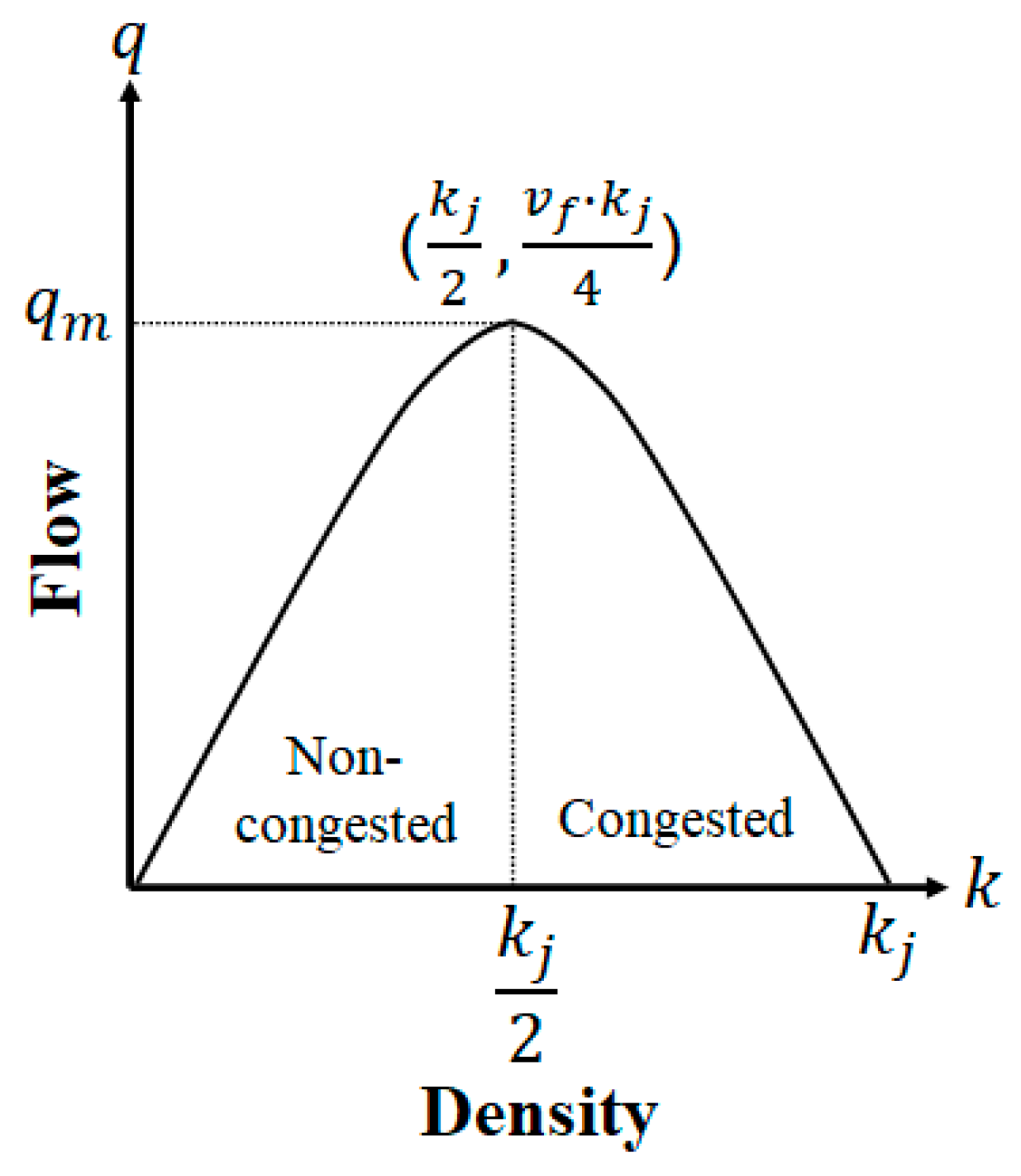
The Greenshields model has been widely used to study highway traffic conditions by examining the relationships among traffic flow, density, and vehicle speed. Owing to its simplicity, this model has been extensively applied in traffic flow prediction, road design, and traffic management [17]. Generally, the highway traffic status can be classified into two modes: congested mode and non-congested mode. In the congested mode, traffic has reached saturation, where an excessively high vehicle density causes significant congestion and a sharp reduction in travel speed. In contrast, the non-congested mode refers to conditions where vehicles move at a relatively low density and high speed, resulting in smooth and unobstructed flow. In the Greenshields model, the relationship between traffic flow $q\left(k\right)$ and vehicle density $k$ primarily describes how the traffic flow varies as the vehicle density changes across a road segment. This relationship can be expressed as [17]

$$q(k)=k·v_f-\left[{\displaystyle \frac{v_f}{k_j}}\right]k^2,$$

(1)

where $q\left(k\right)$ denotes the traffic flow, $k$ is the vehicle density, $v_f$ is the free-flow speed, and $k_j$ is the jam density parameter. The flow–density relationship curve is illustrated in Figure 2.

Based on measurements of uninterrupted traffic flow on highways, the Greenshields model expresses the relationship between vehicle speed and density as [17]

$$v(k)=v_f-\left[{\displaystyle \frac{v_f}{k_j}}\right]·k,$$

(2)

where $v\left(k\right)$ is the average vehicle speed, $k$ is the average vehicle density, $v_f$ is the free-flow speed, and $k_j$ represents the density parameter. The speed–density curve corresponding to this model is shown in Figure 3.

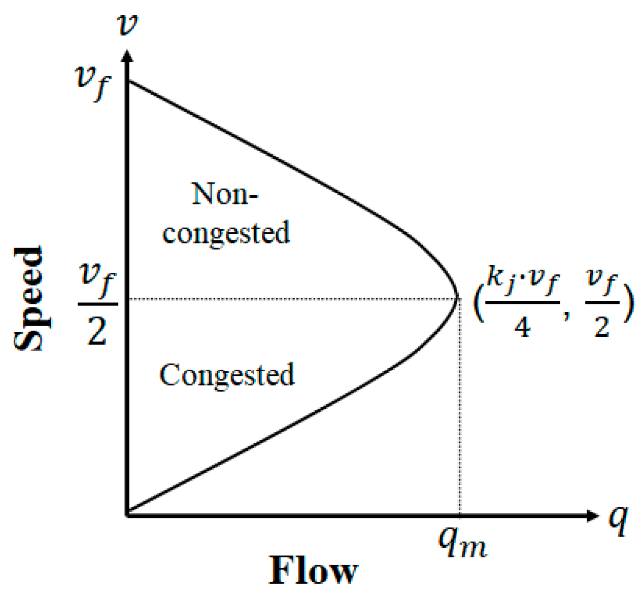
The Greenshields speed–flow relationship curve illustrates how the average vehicle speed varies with an increasing traffic volume on highways. This relationship can be expressed as [17]

$$q(v)=v{·k}_j-\left[{\displaystyle \frac{k_j}{v_f}}\right]v^2,$$

(3)

where $q\left(v\right)$ is the traffic flow and $v$ is the average vehicle speed, $v_f$ is the free-flow speed, and $k_j$ is the density parameter. The corresponding speed–flow curve is shown in Figure 4.

Based on the traffic relationships from Greenshields models, one can evaluate the designs of different highly efficient traffic control and management schemes that can alleviate congestion. It has also been extensively used and validated in subsequent traffic engineering research.

2.3. Setup of Models Using Regression Analysis

Regression analysis is a statistical method that uses mathematical computations on large volumes of data to explain and predict relationships between variables. To determine the correlation between dependent and independent variables, polynomial regression involves deriving suitable regression coefficients, establishing regression equations, and calculating confidence intervals for predicted values. Greenshields models for highway traffic can be developed through regression analysis for time-series forecasting by fitting polynomial equations to the collected traffic data. A polynomial curve of degree $n$, obtained through regression analysis, can be expressed as [43]

$$Y={\alpha }_0+{\alpha }_{1}X+{\alpha }_2{X}^2+\cdots +{\alpha }_n{X}^n+ϵ,$$

(4)

where $Y$ is the dependent variable, $X$ is the independent variable, ${\alpha }_0$ is the intercept, ${\alpha }_1,{\alpha }_2,\dots ,{\alpha }_n$ are the polynomial coefficients, and $ϵ$ is the error term. The curvature of the model and its ability to fit the data depend on the chosen polynomial degree $n$. Polynomial regression fits a polynomial equation to the data, enabling an estimation of the dependent variable for any given independent variable within the data range. Although this method is straightforward, selecting the appropriate polynomial degree is critical and should be based on the data characteristics and the desired accuracy. If the degree is too high, the model may overfit the data, capturing noise and providing a poor representation of the true relationship.

For irregularly spaced or highly variable data, nonlinear regression analysis using a specified response function can offer a more suitable alternative. The nonlinear regression equation for establishing such a model can be expressed as [27,44]

$$Y=f\left(X,\mu \right)+ϵ,$$

(5)

where $f(X,\mu )$ is the response function, $\mu$ represents the parameters, and $ϵ$ is the error term. The parameters $\mu$ in the regression equation can be determined using the least squares estimation (LSE) method. This approach involves multiple iterations to test different parameter values. The key objective is to find the values of $\mu$ that minimize the cost function based on the sample data, thereby optimizing the model’s fit to the data.

2.4. Fuzzy Logic System Model Setup

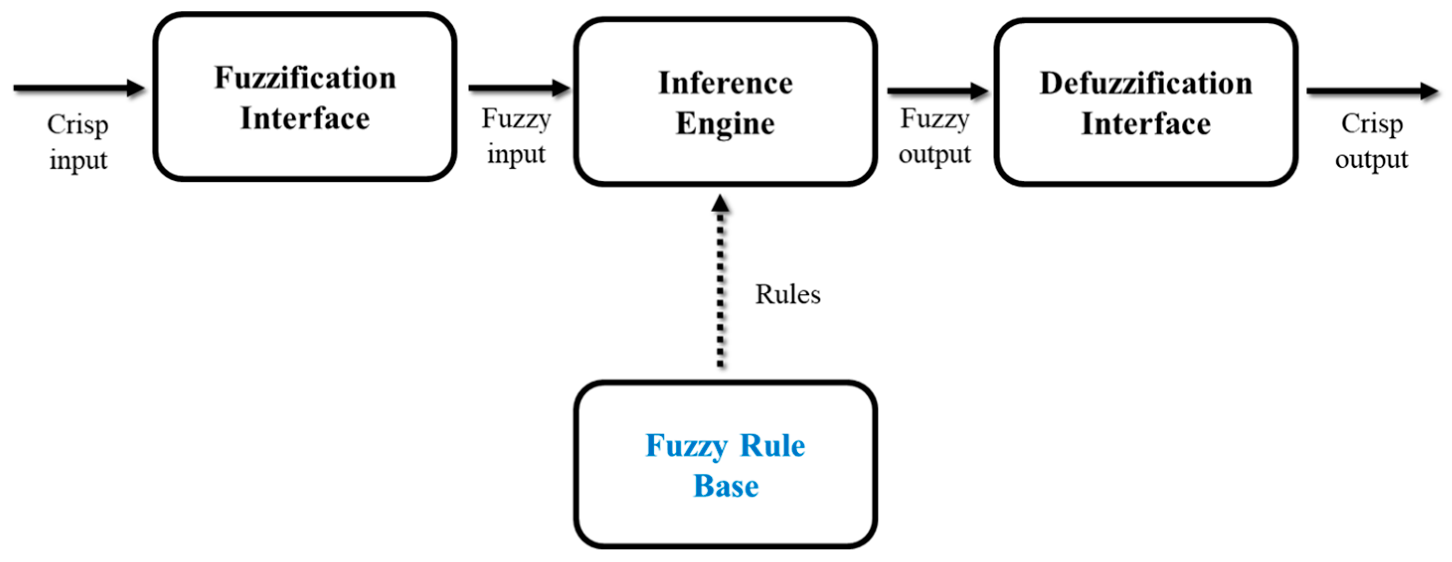
Fuzzy logic is widely applied in artificial intelligence, control systems, decision analysis, pattern recognition, and other fields [45,46]. The basic structure of a fuzzy logic system consists of four key components: fuzzification, the inference engine, the fuzzy rule base, and defuzzification, as illustrated in Figure 5.

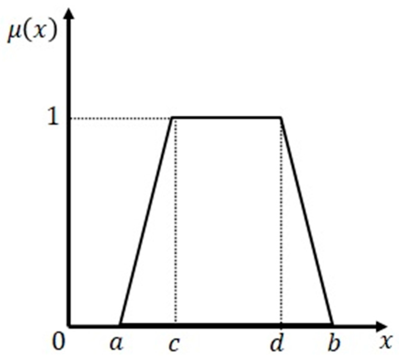
The membership function in fuzzy logic describes the degree of membership of an element within a fuzzy set, where the degree indicates how strongly the element fits the characteristics of that set. The trapezoidal membership function, defined by four parameters $\left(a,b,c,d\right)$, is commonly used in many applications, as shown in Figure 6. It can be expressed by (6), where points $a$ and $b$ represent the start and end of the range with zero membership value, while points $c$ and $d$ define the vertices of the trapezoid where the membership value reaches its maximum. These parameters determine the shape of the trapezoid and the corresponding membership values of the fuzzy set [46].

$$\mu \left(x\right)=\left\{\begin{array}{cc}0,& x<a\\ {\displaystyle \frac{x-a}{c-a}},& x\in \left[a,c\right]\\ 1,& x\in \left[c,d\right]\\ {\displaystyle \frac{b-x}{b-d}},& x\in \left[d,b\right]\\ 0,& x>b\end{array}\right..$$

(6)

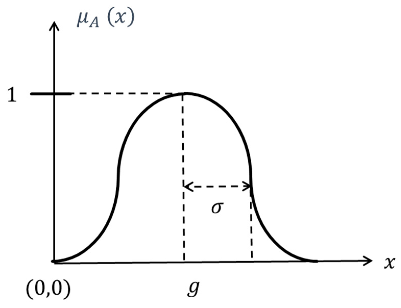
The Gaussian membership function is another frequently used type. Its graph is shown in Figure 7, defined by two parameters: $g$, which determines the center and peak of the curve, and $\sigma$, which controls the width. The general Gaussian membership function can be expressed by [46]

$${\mu }_A\left(x\right)=e^{{-{\displaystyle \frac{1}{2}}\left({\displaystyle \frac{x-g}{\sigma }}\right)}^2}.$$

(7)

Fuzzy rules establish an inference mechanism based on fuzzy logic, linking input and output variables through linguistic terms and fuzzy sets. These rules typically employ conditional statements with logical operators to perform fuzzy reasoning on fuzzy inputs, producing fuzzy outputs. By capturing the relationships between inputs and outputs, fuzzy rules enable flexible decision-making, which is essential in many control systems and artificial intelligence applications. The algorithm for fuzzy logic systems generally adopts an if-then clause structure, which can be written as [46]

$$\mathrm{If}(x_1\left)\mathrm{is}\right(A_1)\mathrm{and}\dots \mathrm{and}(x_i\left)\mathrm{is}\right(A_i\left)\mathrm{then}\right(y\left)\mathrm{is}\right(B),i=1,2,3\dots ,n,$$

(8)

where $x_i$ are input parameters, $y$ is the output parameter, $A_i$ are the assumed conditions, $B$ is the corresponding action based on these conditions, and $n$ is the number of rules. Fuzzy rules also employ fuzzy logic operators such as AND, OR, and NOT to manage operations between fuzzy sets through a consistent and reasonable inference process, improving the system’s accuracy and adaptability.

Defuzzification is the final stage of the fuzzy logic system. It converts the inferred fuzzy results into a precise numerical output $y\left(x\right)$. Typically, this output represents the center of area (COA) of the aggregated output membership function and is calculated as [46]

$$y\left(x\right)={\displaystyle \frac{\sum _{i=1}^N{y}_i\mu \left(y_i\right)}{\sum _{i=1}^N\mu \left(y_i\right)}},$$

(9)

where $y_i$ is the output value of rule $i$, and $\mu \left(y_i\right)$ is the corresponding membership degree of $y_i$.

3. Cascaded Fuzzy Systems Based on Greenshields Models for Vehicle Speed and Travel-Time Prediction

The relationship among vehicle speed, traffic flow, and traffic density on highways can be described by Greenshields models. This study focuses on the design and implementation of a fuzzy logic system for vehicle speed prediction based on Greenshields models. In the proposed approach, traffic flow and traffic density serve as input parameters, with their corresponding membership functions defined according to realistic traffic conditions. A fuzzification process transforms these inputs into meaningful fuzzy values based on the specified membership functions. The fuzzy inference mechanism then applies logical rules derived from Greenshields models to the input information, establishing decision-making laws for predicting vehicle speed as the output parameter. In the defuzzification stage, the centroid method is employed to convert the fuzzy inference results into a precise vehicle speed prediction. For practical application, the models were developed using traffic data from the southern section of the Sun Yat-Sen Highway, specifically the segment between the Dingjin System and the Rende System. The speed limit for passenger cars on this highway ranges from 60 to 110 km/h, with a buffer zone permitting speeds up to 120 km/h. Traffic flow and density data were obtained from the Freeway Bureau [42] and integrated into the model design to ensure that the simulation results are stable and representative of actual traffic conditions. Cascading fuzzy systems in sequence along each highway section enables both vehicle speed prediction and travel-time estimation for specified distances. The procedure for designing the fuzzy logic system is illustrated in Figure 8. Finally, we constructed an additional model using polynomial regression based on the collected data and compared its performance with that of the fuzzy logic model to verify the feasibility of the proposed approach.

3.1. Input and Output Membership Functions’ Setup for Greenshields Model-Based Fuzzy Logic Systems

In fuzzy logic systems, the choice of membership function type depends on the specific application, data characteristics, and desired system behavior. There is no universally optimal function; rather, the goal is to select one that best captures the linguistic terms and relationships within the system. After several trials, we found that trapezoidal membership functions offer the best balance. Regarding the number of levels used in the membership functions for traffic density and flow, there is no single correct value. The selection process is problem-specific and often relies on practical experience and experimentation to achieve the best fit. The number of linguistic variables is typically determined by the level of resolution required in the system’s behavior. After testing several configurations, we identified an appropriate number of levels that achieves a trade-off between model complexity and parameter tuning effort, while closely aligning with the ideal model performance.

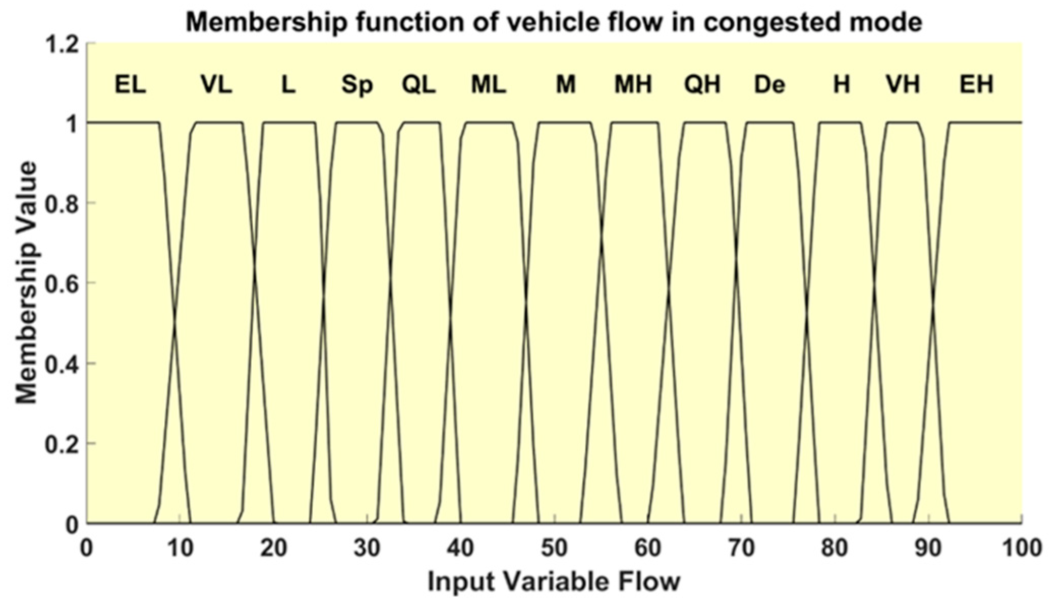
The proposed fuzzy logic system is designed to account for two traffic conditions: congested and non-congested. In each condition, traffic flow and traffic density serve as input parameters, while vehicle speed is the output parameter. Traffic flow is defined as the number of vehicles passing through a road section per hour (veh/h), with its range expressed as a percentage of the specified full flow. Vehicle density refers to the number of vehicles per kilometer on a road section (veh/km), also expressed as a percentage of the specified full density. Vehicle speed represents the rate at which vehicles travel on the road (km/h), with a parameter range from 0 km/h to 130 km/h. Trigonometric or trapezoidal membership functions are chosen for the fuzzy sets, with ambiguous regions specified based on the domain range of collected data and constraints of each highway section. The fuzzy system, with two input parameters and one output parameter, operates in two modes: a congested mode and non-congested mode. In the congested mode, and to align with the Greenshields models, the input membership function for traffic flow is subdivided into thirteen levels to ensure adequate accuracy of the fuzzy logic model. These levels are Extremely Low (EL), Very Low (VL), Low (L), Sparse (Sp), Quite Low (QL), Moderately Low (ML), Moderate (M), Moderate High (MH), Quite High (QH), Dense (De), High (H), Very High (VH), and Extremely High (EH), as presented in

Table 1. Membership function of traffic flow and its range values in congested mode.

Traffic Flow (veh/h)	Percentage of Traffic Flow (%)
Extremely Low (EL)	0~11
Very Low (VL)	8~20
Low flow (L)	17~26
Sparse (Sp)	24~34
Quite Low (QL)	31~40
Moderately Low (ML)	38~48
Moderate (M)	46~57
Moderate High (MH)	53~64
Quite High (QH)	60~71
Dense (De)	69~78
High (H)	76~86
Very High (VH)	83~92
Extremely High (EH)	89~100

. The membership function and its range for traffic flow in the congested mode are illustrated in Figure 9.

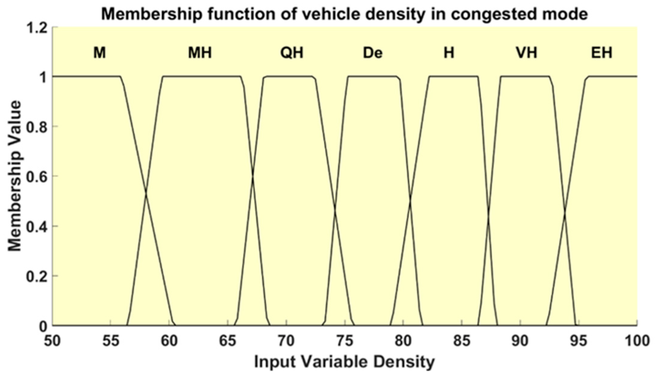
For traffic density in the congested mode, the fuzzy domain is divided into the following levels: Moderate (M), Moderate High (MH), Quite High (QH), Dense (De), High (H), Very High (VH), and Extremely High (EH), as detailed in

Table 2. Membership function of traffic density and its range values in congested mode.

Traffic Density (veh/km)	Percentage of Density (%)
Moderate (M)	50~60
Moderate High (MH)	57~68
Quite High (QH)	66~76
Dense (De)	73~82
High (H)	80~88
Very High (VH)	87~95
Extremely High (EH)	92~100

. The corresponding membership function and range are shown in Figure 10.

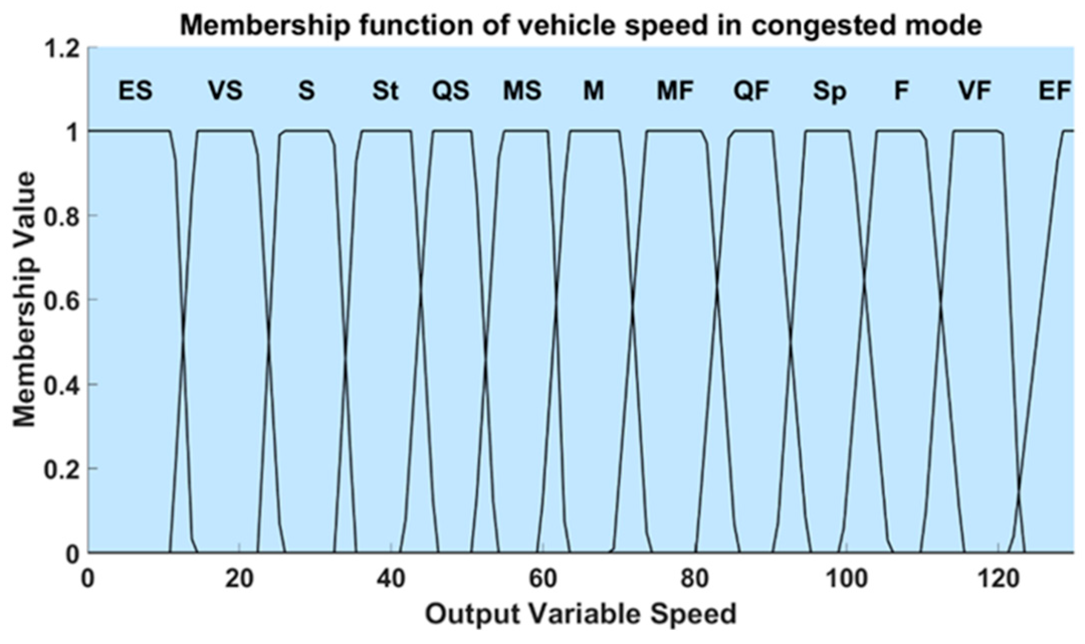
The fuzzy domain of the output membership function for vehicle speed includes the following levels: Extremely Slow (ES), Very Slow (VS), Slow (S), Steady (St), Quite Slow (QS), Moderate Slow (MS), Moderate (M), Moderate Fast (MF), Quite Fast (QF), Speedy (Sp), Fast (F), Very Fast (VF), and Extremely Fast (EF), as presented in

Table 3. Membership function of vehicle speed and its range values in congested mode.

Vehicle Speed (km/h)	Mapping Interval (km)
Extremely Slow (ES)	0~14
Very Slow (VS)	11~26
Slow (S)	22~35
Steady (St)	33~46
Quite Slow (QS)	42~54
Moderate Slow (MS)	51~63
Moderate (M)	60~74
Moderate Fast (MF)	69~85
Quite Fast (QF)	80~95
Speedy (Sp)	91~106
Fast (F)	99~115
Very Fast (VF)	110~123
Extremely Fast (EF)	122~130

. The membership function and its range for vehicle speed are depicted in Figure 11.

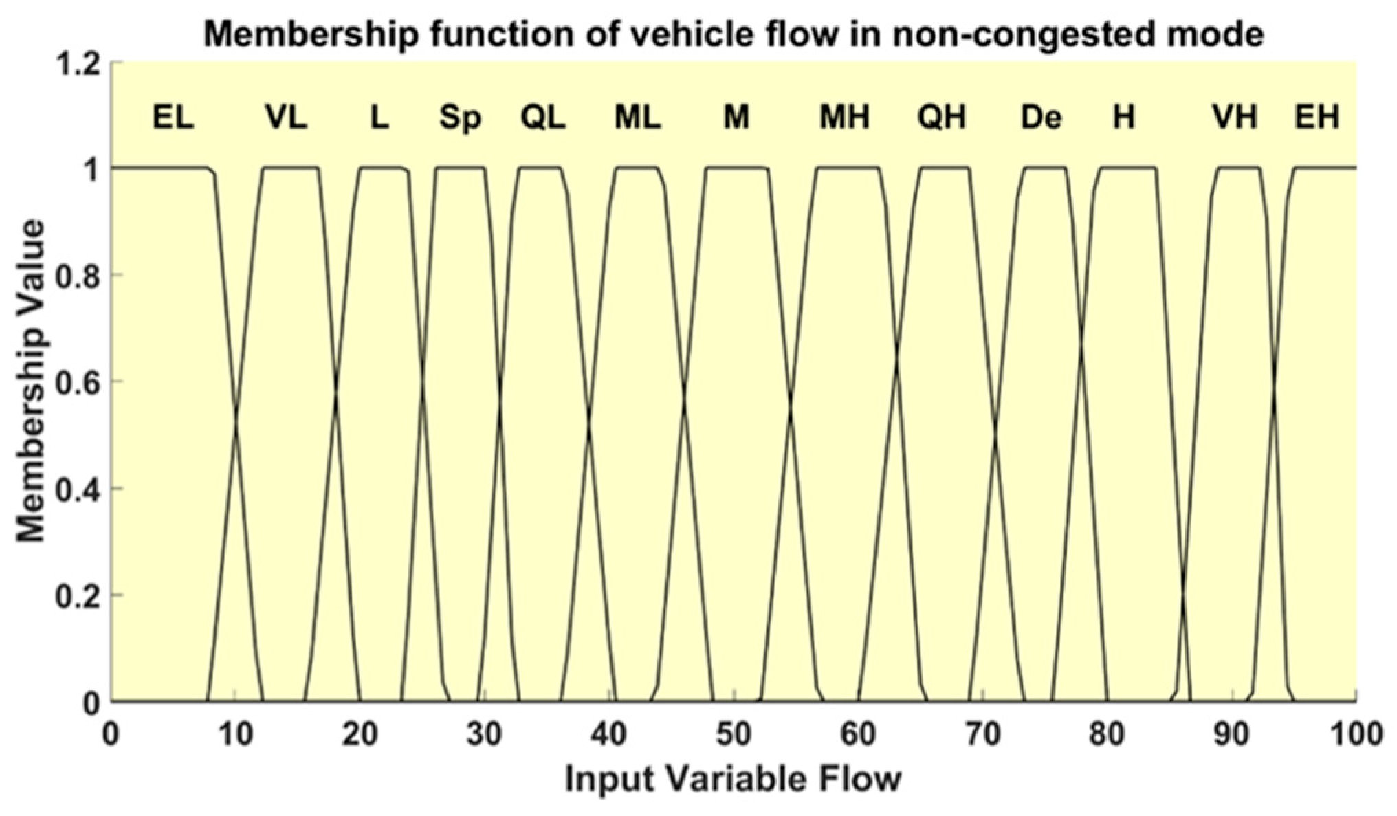
For the non-congested mode, the fuzzy domain of the membership functions for traffic flow is divided into the following levels: Extremely Low (EL), Very Low (VL), Low (L), Sparse (Sp), Quite Low (QL), Moderately Low (ML), Moderate (M), Moderate High (MH), Quite High (QH), Dense (De), High (H), Very High (VH), and Extremely High (EH), as presented in

Table 4. Membership function of traffic flow and its range values in non-congested mode.

Traffic Flow (veh/h)	Percentage of Traffic Flow (%)
Extremely (EL)	0~12
Very Low (VL)	8~20
Low (L)	16~27
Sparse (Sp)	23~32
Quite Low (QL)	30~40
Moderately Low (ML)	36~48
Moderate (M)	44~57
Moderate High (MH)	52~65
Quite High (QH)	60~73
Dense (De)	69~80
High (H)	76~87
Very High (VH)	86~95
Extremely High (EH)	92~100

. The membership function and range values for traffic flow in the non-congested mode are illustrated in Figure 12.

Similarly, the fuzzy domain of the membership function for traffic density in the non-congested mode is segmented into seven levels: Extremely Low (EL), Very Low (VL), Low (L), Sparse (Sp), Quite Low (QL), Moderately Low (ML), and Moderate (M), as detailed in

Table 5. Membership function of traffic density and its range values in non-congested mode.

Traffic Density (veh/km)	Percentage of Density (%)
Extremely Low (EL)	0~10
Very Low (VL)	7~17
Low (L)	14~25
Sparse (Sp)	22~31
Quite Low (QL)	26~39
Moderately Low (ML)	34~45
Moderate (M)	42~50

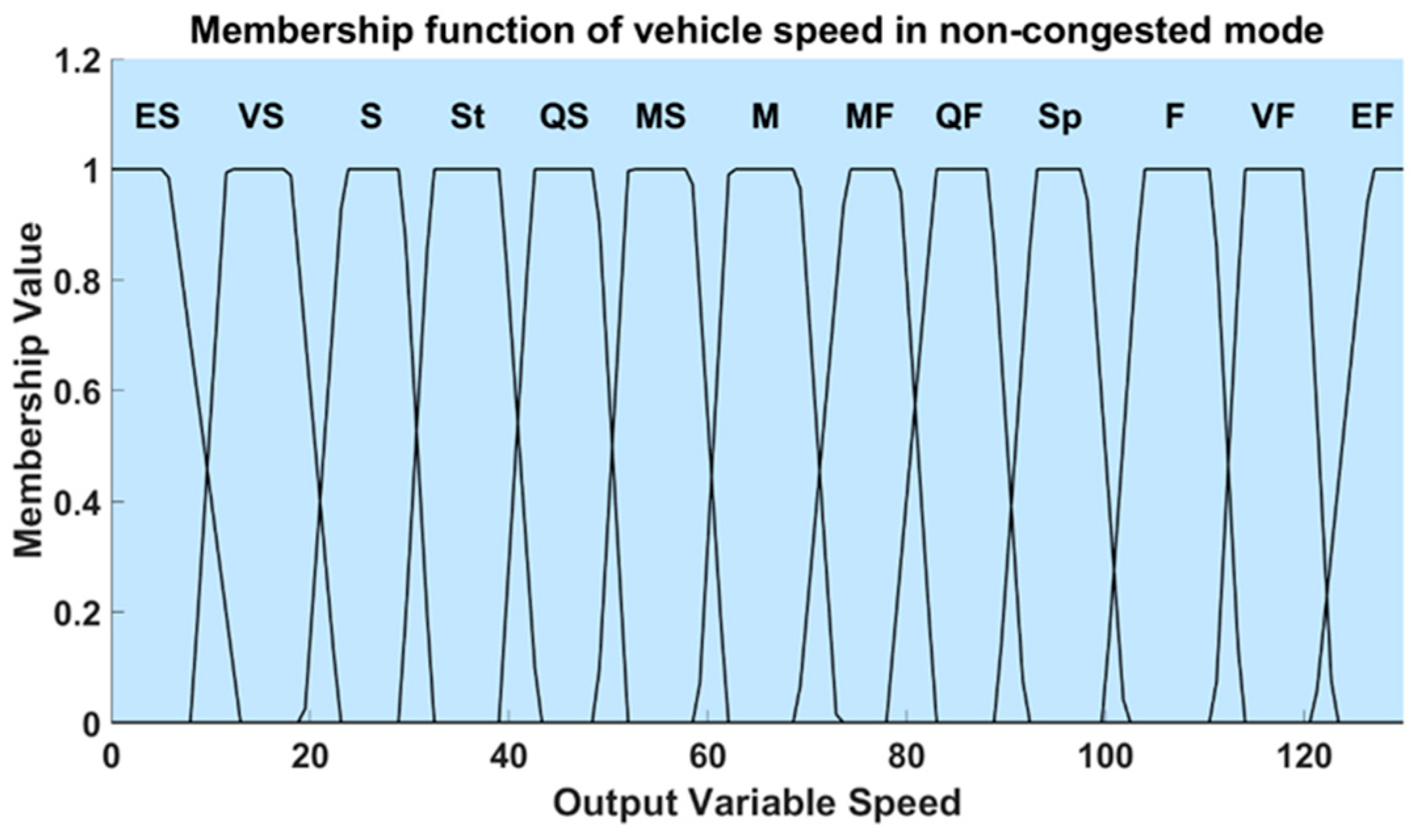
. The membership function and range values for traffic density are shown in Figure 13. The fuzzy domain of the output membership function for vehicle speed in the non-congested mode is defined by the following levels: Extremely Slow (ES), Very Slow (VS), Slow (S), Steady (St), Quite Slow (QS), Moderate Slow (MS), Moderate (M), Moderate Fast (MF), Quite Fast (QF), Speedy (Sp), Fast (F), Very Fast (VF), and Extremely Fast (EF), as presented in

Table 6. Membership function of vehicle speed and its range values in non-congested mode.

Vehicle Speed (km/h)	Mapping Interval (km)
Extremely Slow (ES)	0~13
Very Slow (VS)	8~23
Slow (S)	19~32
Steady (St)	29~43
Quite Slow (QS)	39~52
Moderate Slow (MS)	49~62
Moderate (M)	59~73
Moderate Fast (MF)	69~83
Quite Fast (QF)	78~92
Speedy (Sp)	89~102
Fast (F)	100~114
Very Fast (VF)	111~123
Extremely Fast (EF)	121~130

. The membership function and its corresponding range for vehicle speed are depicted in Figure 14.

3.2. Inference Rule and Defuzzification

To establish the fuzzy inference relationship between inputs and outputs, a fuzzy rule base grounded in Greenshields theory is developed to capture the relationships among traffic flow, density, and vehicle speed, thereby reflecting real traffic conditions. In this study, T-norms are primarily used to perform fuzzy set logic operations, supporting the construction of fuzzy rules and inference processes to assess the similarity between fuzzy sets. Within the fuzzy rules, the intersection of fuzzy sets is represented by the minimum value, while the union operation expresses the degree of inclusiveness between two fuzzy sets using the maximum value. Two separate fuzzy rule sets are formulated for congested and non-congested conditions, as detailed in

Table 7. Fuzzy logic rule set in congested mode.

	Vehicle Flow		Traffic Density		Vehicle Speed
If	EL	OR	EH	Then	ES
If	EL	AND	VH	Then	ES
If	EL	OR	H	Then	VS
If	VL	OR	EH	Then	ES
If	VL	AND	VH	Then	VS
If	VL	OR	H	Then	S
If	L	AND	EH	Then	VS
If	L	OR	VH	Then	VS
If	L	AND	H	Then	S
If	Sp	OR	EH	Then	VS
If	Sp	AND	VH	Then	S
If	Sp	OR	H	Then	S
If	QL	OR	VH	Then	S
If	QL	OR	H	Then	S
If	QL	AND	De	Then	S
If	ML	OR	VH	Then	S
If	ML	OR	H	Then	S
If	ML	AND	De	Then	St
If	M	AND	VH	Then	S
If	M	AND	H	Then	St
If	M	AND	De	Then	St
If	MH	OR	H	Then	St
If	MH	AND	Dense	Then	St
If	MH	OR	QH	Then	QS
If	QH	AND	H	Then	St
If	QH	AND	De	Then	QS
If	QH	AND	QH	Then	QS
If	De	AND	De	Then	QS
If	De	OR	QH	Then	QS
If	De	OR	MH	Then	MS
If	H	AND	De	Then	MS
If	H	OR	QH	Then	MS
If	H	OR	MH	Then	MS
If	VH	OR	QH	Then	MS
If	VH	AND	MH	Then	MS
If	VH	OR	M	Then	M
If	EH	OR	QH	Then	MS
If	EH	OR	MH	Then	M
If	EH	OR	M	Then	M

and

Table 8. Fuzzy logic rule set in non-congested mode.

	Traffic Flow		Traffic Density		Vehicle Speed
If	EL	OR	EL	Then	EF
If	EL	AND	VL	Then	EF
If	EL	AND	L	Then	VF
If	VL	OR	EL	Then	EF
If	VL	OR	VL	Then	VF
If	VL	AND	L	Then	F
If	L	AND	EL	Then	VF
If	L	OR	VL	Then	VF
If	L	AND	L	Then	F
If	Sp	OR	EL	Then	VF
If	Sp	AND	VL	Then	VF
If	Sp	AND	L	Then	F
If	QL	OR	VL	Then	F
If	QL	OR	L	Then	F
If	QL	AND	Sp	Then	F
If	ML	OR	VL	Then	F
If	ML	OR	L	Then	Sp
If	ML	AND	Sp	Then	Sp
If	M	AND	VL	Then	F
If	M	AND	L	Then	Sp
If	M	AND	Sp	Then	Sp
If	MH	OR	L	Then	Sp
If	MH	AND	Sp	Then	Sp
If	MH	OR	QL	Then	QF
If	QH	AND	L	Then	Sp
If	QH	AND	Sp	Then	QF
If	QH	AND	QL	Then	QF
If	De	AND	Sp	Then	Sp
If	De	OR	QL	Then	QF
If	De	OR	ML	Then	MF
If	H	AND	Sp	Then	QF
If	H	OR	QL	Then	QF
If	H	OR	ML	Then	MF
If	VH	OR	QL	Then	MF
If	VH	AND	ML	Then	MF
If	VH	OR	M	Then	M
If	EH	AND	QL	Then	MF
If	EH	AND	ML	Then	MF
If	EH	AND	M	Then	M

. The tabular representation of these rule sets helps ensure consistency, prevents contradictions, and avoids illogical rules that would not align with real-world highway traffic conditions, thereby supporting accurate vehicle speed prediction.

In the final stage of the Greenshields-based fuzzy logic system, defuzzification converts the fuzzy outputs into specific numerical values for further analysis and application. The centroid method is employed in the defuzzification process to calculate the center of the fuzzy result region, yielding a definitive and interpretable vehicle speed value.

3.3. Cascaded Fuzzy Logic Systems for Travel-Time Prediction

Since Greenshields models are derived from short-range data collection and analysis, the proposed fuzzy logic system for vehicle speed prediction is effective for specific highway segments. As drivers typically travel along routes composed of several consecutive segments, each segment is equipped with its own dedicated fuzzy logic system for speed prediction. To enable travel-time prediction for an entire route leading to a destination, multiple fuzzy subsystems—each based on the Greenshields model—are linked together in series to form a cascaded system. As illustrated in the flowchart of Figure 15, each pair of consecutive fuzzy logic subsystems corresponds to two sequential highway segments. Each subsystem receives current traffic flow and density data from its respective prediction scheme as inputs. Through fuzzy logic processing, the subsystem predicts the vehicle speed for that segment. Using the predicted speed, the travel time for the segment can then be estimated.

By cascading multiple fuzzy logic subsystems, each with traffic flow and density as inputs and vehicle speed as outputs, complex parameter relationships across a long-range route with multiple segments can be handled and analyzed in real-time, enabling accurate travel-time prediction for long-distance highway paths. An example of the cascaded fuzzy logic system, consisting of four subsystems for current highway traffic status prediction, is shown in Figure 16. Each subsystem predicts the vehicle speed for its corresponding segment, and the required travel time for each segment is then calculated. By summing the travel times for all segments, the estimated total travel time for the specified journey is obtained, with real-time updates based on the current status of the highway.

The cascaded fuzzy logic system, designed for multiple specified segments, integrates, processes, and updates varying traffic information, thereby improving the accuracy of real-time highway travel-time predictions. This approach not only allows for the processing of long-range traffic data but also dynamically adjusts the predicted travel time in response to changing traffic conditions, enhancing the system’s flexibility and adaptability.

4. Simulation Results and Discussions

In this section, simulations of the proposed Greenshields model-based fuzzy logic system for vehicle speed and travel-time prediction are conducted using traffic data from a specified segment of the Sun Yat-Sen Highway in Taiwan. These simulations aim to demonstrate the reliability and effectiveness of the developed fuzzy logic models. For comparison, a conventional model is also established using regression analysis. The proposed cascaded system for long-range travel-time prediction is likewise verified through simulation. The discussion of simulation results provides valuable insights that confirm the feasibility of the proposed system for vehicle speed prediction. The simulations ultimately validate the system’s accuracy, its capability to enhance prediction performance, and its flexibility in constructing a cascaded fuzzy logic system for travel-time prediction across long-range routes composed of multiple highway segments.

4.1. Highway Vehicle Speed Prediction Using Greenshields Models Based Fuzzy Logic System

Traffic status data, including traffic flow and traffic density, collected from the segment between Dingjin and Rende on the Sun Yat-Sen Highway in Taiwan [42], are used to illustrate the design of Greenshields model-based fuzzy logic systems for dual-mode vehicle speed prediction. Separate fuzzy systems are developed for congested and non-congested modes to model the relationships among traffic flow, traffic density, and vehicle speed. To build an effective fuzzy system, the variable ranges are defined based on empirical data, and the model parameters are adjusted to align with actual traffic conditions on the specified highway segment.

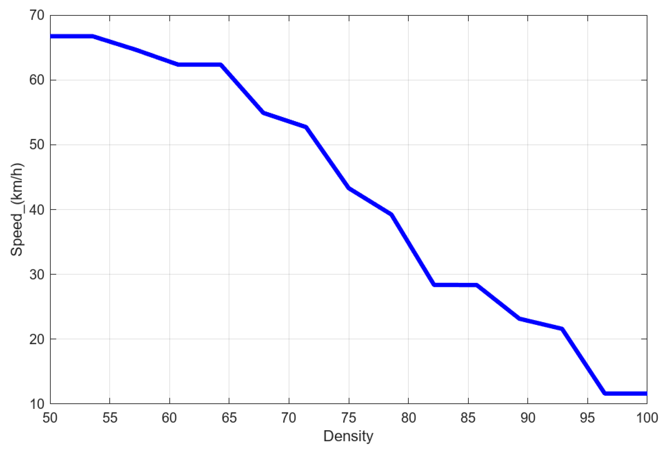
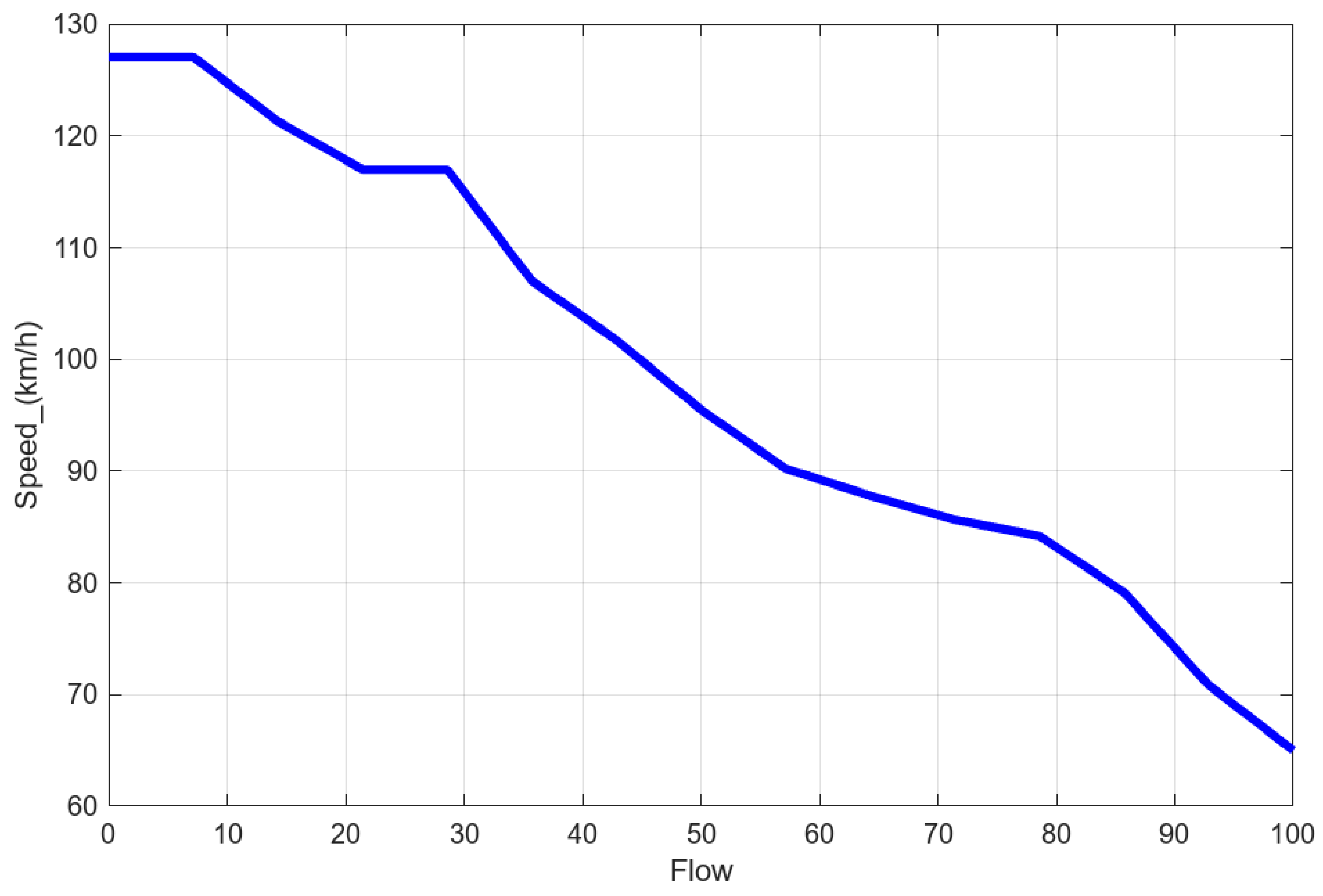
The simulations are performed using MATLAB_R2021b, which provides a visual interface for adjusting parameter values during model setup and for dynamically evaluating the performance of the fuzzy logic system throughout the design process. In the design specifications, the two input variables—traffic flow and traffic density—are expressed as percentages, ranging from 0% to 100% of their respective maximum values on the segment. The output variable, vehicle speed, ranges from 0 to 130 km/h. The relationship between vehicle speed and traffic density in the congested mode is shown in Figure 17, displaying a linear correlation consistent with the theoretical model in Figure 3. The relationship between vehicle speed and traffic flow in the congested mode is depicted in Figure 18, illustrating a quadratic relationship that corresponds to the theoretical model in Figure 4. Similarly, the curve of vehicle speed versus traffic density and the graph of vehicle speed versus traffic flow in the non-congested mode are presented in Figure 19 and Figure 20, respectively.

The results show that the fuzzy logic models are highly consistent with Greenshields’ theoretical models. Moreover, the dual-mode fuzzy logic system provides valuable insight into the dynamic traffic status at specific locations. Using this system, real-time vehicle speeds can be accurately predicted, closely approximating actual conditions. These results confirm the feasibility and effectiveness of the proposed scheme.

Fuzzy logic is a mathematical framework for dealing with vague or ambiguous information. It allows for the representation of imprecise data and the use of linguistic variables. Fuzzy logic systems employ fuzzy rules to capture expert knowledge and express connections between factors. Hence, fuzzy logic is suitably used in systems where precise mathematical modeling is difficult.

4.2. Greenshields Models Based on Regression Analysis

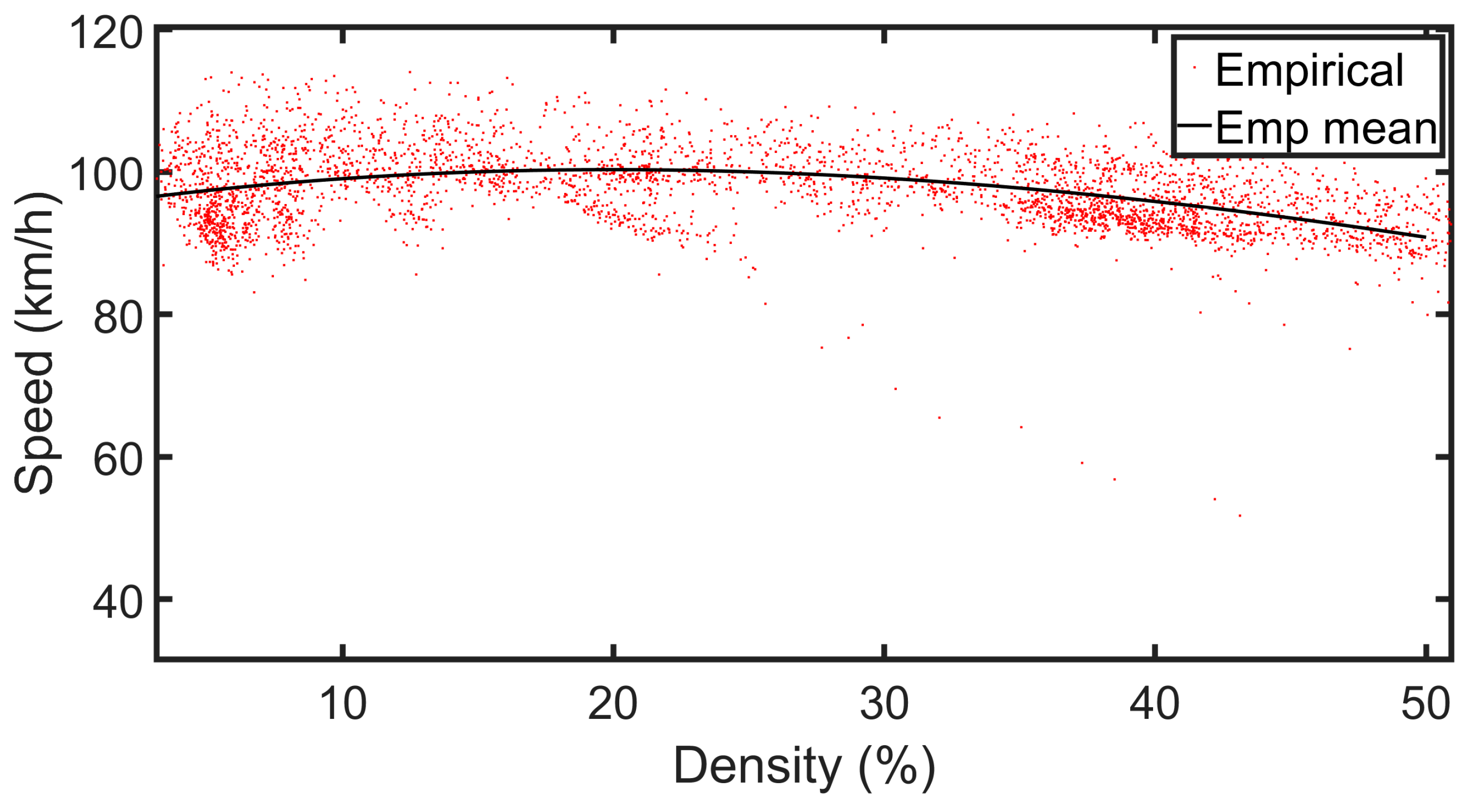
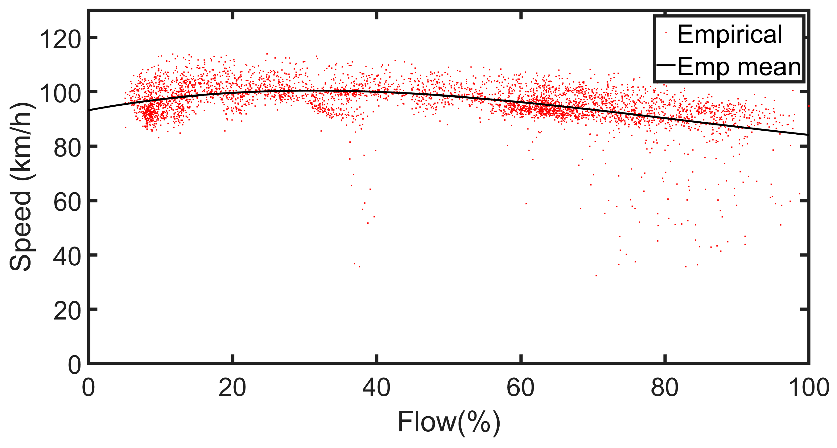
Many regression analysis methods can be applied to establish Greenshields models. In this study, polynomial regression is used to construct models based on traffic data collected from the segment between Dingjin and Rende on the Sun Yat-Sen Highway in Taiwan [42], for validation and comparison with the proposed fuzzy logic system. The regression process extracts key information from the collected data and smooths out noise present in the measurements. The resulting models in the non-congested mode include the relationship curve between vehicle speed and traffic density shown in Figure 21, the graph of traffic flow versus traffic density illustrated in Figure 22, and the diagram of vehicle speed versus traffic flow presented in Figure 23.

To evaluate the model fit and predictive performance of each regression model, statistical analyses were conducted for the regression plots shown in Figure 21, Figure 22 and Figure 23. The corresponding results are summarized in

Table 9. Regression statistics: Vehicle versus traffic density.

Reg Statistics
R Multiple	0.876223
R-Squared	0.867767
R-Squared(Adj)	0.86766
SER	3.825537
DF	2159
ANOVA
Source	DF	SS	MS	F	Levrg Pt
Regression	1	104,361.7	104,361.7	7131.101	0
Error	2157	31,567.11	14.63473
Total	2158	135,928.8
Coefficients
Term	Coef	SE Coef	t-Value	p-Value	Lwr 95%	Upr 95%
${\beta }_0$	105.6728	0.164547	642.2055	0	105.3501	105.9955
${\beta }_1$	−0.50657	0.005999	−84.4458	0	−0.51834	−0.49481

,

Table 10. Regression statistics: Traffic flow versus density.

Reg Statistics
R Multiple	0.981812
R-Squared	0.963955
R-Squared(Adj)	0.963938
SER	210.7215
DF	2159
ANOVA
Source	DF	SS	MS	F	Levrg Pt
Regression	1	2.56 × 109	2.56 × 109	57,685.16	0
Error	2157	95,778,434	44,403.54
Total	2158	2.66 × 109
Coefficients
Term	Coef	SE Coef	t-Value	p-Value	Lwr 95%	Upr 95%
${\beta }_0$	243.7202	9.063705	26.88969	0	225.9457	261.4948
${\beta }_1$	79.36201	0.330431	240.1774	0	78.71401	80.01001

and

Table 11. Regression statistics: Traffic flow versus vehicle speed.

Reg Statistics
R Multiple	0.892857
R-Squared	0.828622
R-Squared(Adj)	0.828449
SER	676.3877
DF	2159
ANOVA
Source	DF	SS	MS	F	Levrg Pt
Regression	1	1.67 × 109	1.67 × 109	3651.092	0
Error	2157	9.87 × 108	457,500.3
Total	2158	2.66 × 109
Coefficients
Term	Coef	SE Coef	T-Value	P-Value	Lwr 95%	Upr 95%
${\beta }_0$	12,509.11	172.4106	72.55417	0	12171	12,847.22
${\beta }_1$	−110.854	1.834594	−60.4243	0	−114.452	−107.256

. While regression slope estimates can be significantly affected by high-leverage points, the collected data show no such influence (leverage point value: 0), indicating the absence of significant outliers. The quality of the slope estimator, as reflected by the standard deviation (SE Coef) of ${\beta }_1$, is influenced by two key factors: the error variance of the mean square error (MS value) and the degree of variability in the independent variable. A higher error variance for a given level of the independent variable makes it more challenging to obtain an accurate estimate of the regression line. Notably, the standard deviation values (SE Coef) of ${\beta }_1$ are small in each model. When compared with their corresponding slope parameter values (Coef), this confirms that the slope estimates are reliable and accurately reflect the underlying process. Similarly, the intercept estimates ${\beta }_0$ also exhibit low standard errors (SE Coef) relative to their parameter values (Coef), indicating minimal extrapolation and enhancing the credibility of the models. $T$-tests were performed on each ${\beta }_1$ parameter, and the resulting $p$-values for the two-tailed tests are effectively zero. This confirms that all slope coefficients are statistically significant. The 95% confidence intervals—specified by the lower (Lwr 95%) and upper (Upr 95%) bounds—for both the intercept and slope values, as reported in Table 9, Table 10 and Table 11, further demonstrate the precision of the estimates and suggest minimal uncertainty. All models also report high $R$-squared ($R^2$) values, approaching 1, indicating a strong fit between the regression line and the observed data. The standard error of the regression (SER) quantifies the average deviation between observed values and the predicted values on the regression line. Each model demonstrates a low SER, indicating a high prediction accuracy. Specifically, in Table 9, the SER for the estimated vehicle speed is 3.83 km/h, confirming a high degree of precision in the speed prediction.

Although the regression analysis can offer a high predictive accuracy with statistically significant coefficients and low standard errors, it is generally a slow and time-consuming process and less adaptable to dynamic traffic conditions. When conditions or the environment change, new parameters or parameter updates require a substantial amount of additional data for retraining. Despite these limitations, regression models are valuable for examining and verifying the relationships among variables. According to Greenshields’ theory, each curve provides useful insights into the relationships between vehicle speed and traffic density, traffic flow and density, and vehicle speed and traffic flow. The Greenshields models constructed through regression for the specified road segment serve as important references for validating the fuzzy logic system, evaluating its performance, and guiding model parameter adjustments.

4.3. Vehicle Speed Prediction: Tests and Discussion

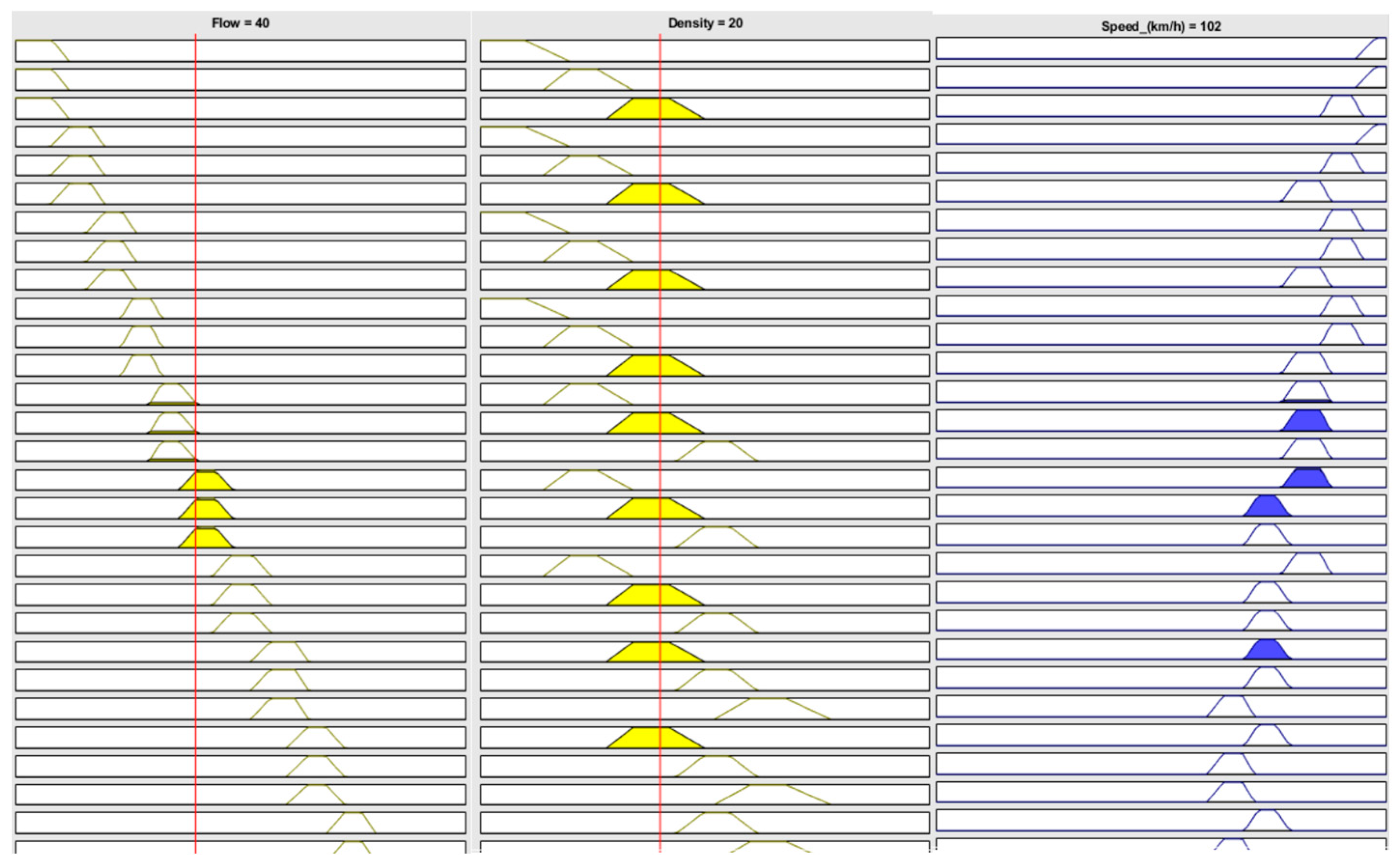
A realistic simulation test in the non-congested mode was conducted using the proposed fuzzy logic system. In this test, the traffic flow input parameter was set at 40% of its maximum value, and the traffic density was set at 20%. When these parameters were fed into the fuzzy logic system, the predicted vehicle speed was approximately 102 km/h, as shown in Figure 24. For comparison, the polynomial regression model in Figure 23 predicts a vehicle speed of about 103 km/h at the same traffic flow level (40%), while the regression model in Figure 21 predicts a speed of about 100 km/h at a traffic density of 20% in the non-congested mode. The simulation results confirm the accuracy of the proposed fuzzy logic system in predicting vehicle speed. The predicted speeds are within about 1% of those generated by regression analysis methods in high-fidelity traffic scenarios. This demonstrates that the proposed system provides predictions that closely approximate actual traffic conditions, validating its feasibility for vehicle speed prediction. Another simulation was performed under a “Quite Low” traffic status scenario, where the traffic flow was set at 34% (classified as “Quite Low”) and the traffic density at 20% (classified as “Low”). Using the centroid method for defuzzification, the fuzzy logic system operating in a non-congested mode predicted a vehicle speed of 101 km/h, as shown in Figure 25. This result further confirms the system’s ability to reflect realistic changes in highway traffic conditions.

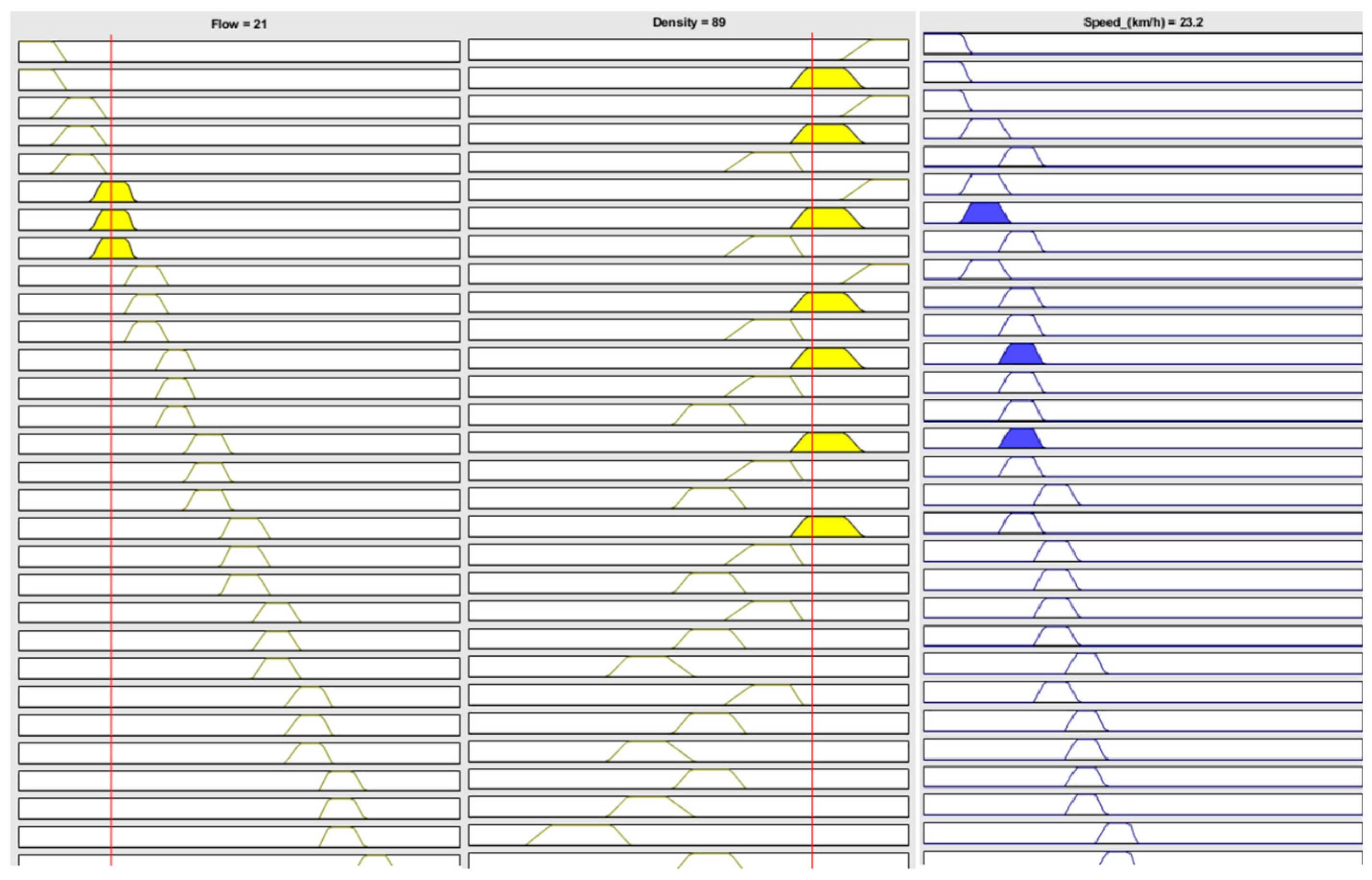
For the test in the congested mode, the input parameters were set with the traffic flow at 21% (classified as “Low”) and the traffic density at 89% (classified as “Very High”). As shown in Figure 26, the fuzzy logic system produced an output vehicle speed of 23.2 km/h. This outcome indicates that under congested conditions, the predicted speed aligns well with actual traffic behavior.

The experimental results indicate that both the fuzzy logic and regression models produce consistent and reliable outputs, confirming the practical feasibility and robustness of the proposed travel-time prediction system. Specifically, the fuzzy logic system effectively applies fuzzy rules to the input values based on their degrees of membership, accurately capturing the complex relationships among vehicle speed, traffic flow, and traffic density to generate meaningful predictions. Overall, the simulation results offer valuable insights into traffic behavior under various conditions, reaffirming the flexibility and effectiveness of the designed fuzzy logic system.

4.4. Travel-Time Prediction Using Greenshields Model Based on Cascaded Fuzzy Logic Systems

A simulation test was conducted to evaluate travel-time prediction using cascaded fuzzy logic systems for segments of the Sun Yat-Sen Highway, specifically from the Dingjin System heading north to the Chiayi System during morning rush hours on a typical working day. The route consists of four segments in sequence: Dingjin to Rende, Rende to Tainan, Tainan to Xiaying, and Xiaying to Chiayi. Each segment is equipped with a dedicated Greenshields model-based fuzzy logic system designed in advance for vehicle speed prediction. These fuzzy logic systems receive real-time traffic data—including traffic density and flow—from the Traffic Control Center for their respective segments [42]. Based on these inputs, each system predicts the vehicle speed for its segment. Using the predicted speeds and the known lengths of the segments, the estimated travel time for each segment is calculated. The total estimated travel time for the entire route from Dingjin to Chiayi is then determined by summing the segment travel times. The simulation results are presented in

Table 12. Predicted travel time from Dingjin System to Chiayi System.

Segments of Highway System	Dingjin to Rende Segment	Rende to Tainan Segment	Tainan to Xiaying Segment	Xiaying to Chiayi Segment
Segment Distance (km)	32	15	16	27
Traffic Conditions	Congested	Congested	Non-Congested	Non-Congested
Traffic Flow (%)	21	58	21	67
Traffic Density (%)	85	78	20	25
Predicted Vehicle Speed (Km/h)	28	43	106	85
Predicted Travel Time (Minutes)	68	21	9	19
Total Required Travel Time	1 h and 57 min

, showing the predicted travel times for each segment along with the corresponding traffic conditions. It is important to note that these estimates vary with changing road conditions and must be updated accordingly. The simulation confirms both the feasibility and adaptability of the cascaded fuzzy logic approach. Since each prediction relies on short-range, segment-specific traffic data, the overall travel-time estimate for the planned route demonstrates a high level of accuracy.

5. Conclusions

Accurate travel-time prediction is a fundamental component of ITS, enabling efficient route planning, reducing delays, optimizing traffic flow, and minimizing fuel consumption and environmental impact. This paper proposes a cascaded fuzzy logic system based on the Greenshields traffic flow model for highway travel-time prediction. The system consists of multiple fuzzy inference subsystems, each designed to estimate vehicle speed and travel time for specific highway segments under either congested or uncongested traffic conditions. By leveraging the mathematical relationship among traffic flow, density, and vehicle speed defined by the Greenshields model, each subsystem generates localized, real-time speed estimates that are subsequently integrated to produce long-range travel-time forecasts. Non-parametric approaches, such as machine learning methods, often require extensive data preprocessing and frequent retraining to maintain accuracy. In contrast, parametric models like regression analysis can offer a high predictive accuracy with statistically significant coefficients and low standard errors, but they are generally static and less adaptable to dynamic traffic conditions. The proposed fuzzy logic system overcomes these limitations by effectively handling uncertainty and imprecise input data, without requiring large training datasets. Furthermore, the system’s modular and flexible structure allows easy adjustments to parameters, making it highly scalable and well-suited for dynamic, data-constrained environments. These characteristics make fuzzy logic a more practical and efficient choice for real-time ITS applications.

Extensive simulations were conducted using traffic data from the Sun Yat-Sen Highway of Taiwan. The fuzzy logic model, tailored for both congested and non-congested scenarios, accurately captured the interrelationships between traffic density, flow, and speed—enabling the system to reflect real-time traffic conditions. To assess the performance of our proposed fuzzy logic system, we compare it with a traditional regression model using the same real-world dataset. In validation tests, the predicted vehicle speeds closely aligned with those generated by polynomial regression models, with discrepancies typically below 1%. The experimental results show that both the fuzzy logic and regression models produce consistent and reliable outputs. Further simulations evaluated the performance of the cascaded fuzzy logic framework for travel-time prediction along a multi-segment route from Dingjin to Chiayi during morning peak hours. Each segment was managed by a dedicated fuzzy logic subsystem, and the total travel time was obtained by summing the predicted times across segments. This segment-wise prediction strategy, based on localized traffic conditions, ensured that the system remained responsive and accurate in the face of evolving traffic patterns. Results demonstrated that the proposed framework effectively captured spatial variations in traffic flow, delivering reliable long-distance travel-time predictions.

In conclusion, by integrating fuzzy logic to develop robust, segment-specific prediction subsystems, the proposed scheme supports key ITS goals, including traffic management, congestion mitigation, and traveler information services. Ultimately, this approach enhances the performance, sustainability, and user satisfaction of highway transportation systems.