
Exploring the Impacts of Yellow Light Duration on Intersection Performance Under Driving Behavior Uncertainty: A Risk Perception and Fuzzy Decision-Based Simulation Framework

Abstract
1. Introduction
- By enhancing the previous risk-perception-based driving behavior model with fuzzy decision-making theory, the micro-level influence of yellow light duration is incorporated into the simulation, further narrowing the gap between simulated and actual driving behaviors.
- A simulation framework employing a set of driving behavior models based on unified modeling logic is integrated, which attempts to eliminate the complexity of switching between different driving behavior models across various road areas and traffic scenarios.
- The process of risk perception grounded in risk homeostasis theory is suggested to explain the underlying mechanisms of traffic flow performance at isolated signalized intersections.
2. Literature Review
3. Risk Perception and Fuzzy Decision-Based Driving Behavior Model
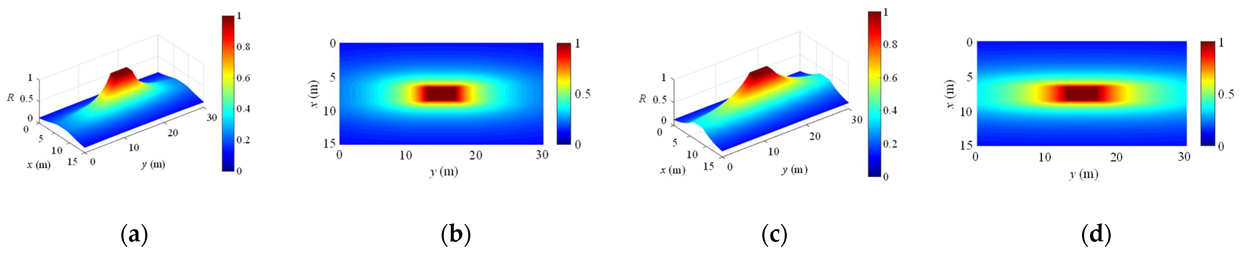
3.1. Risk Quantification
3.2. Risk Prediction
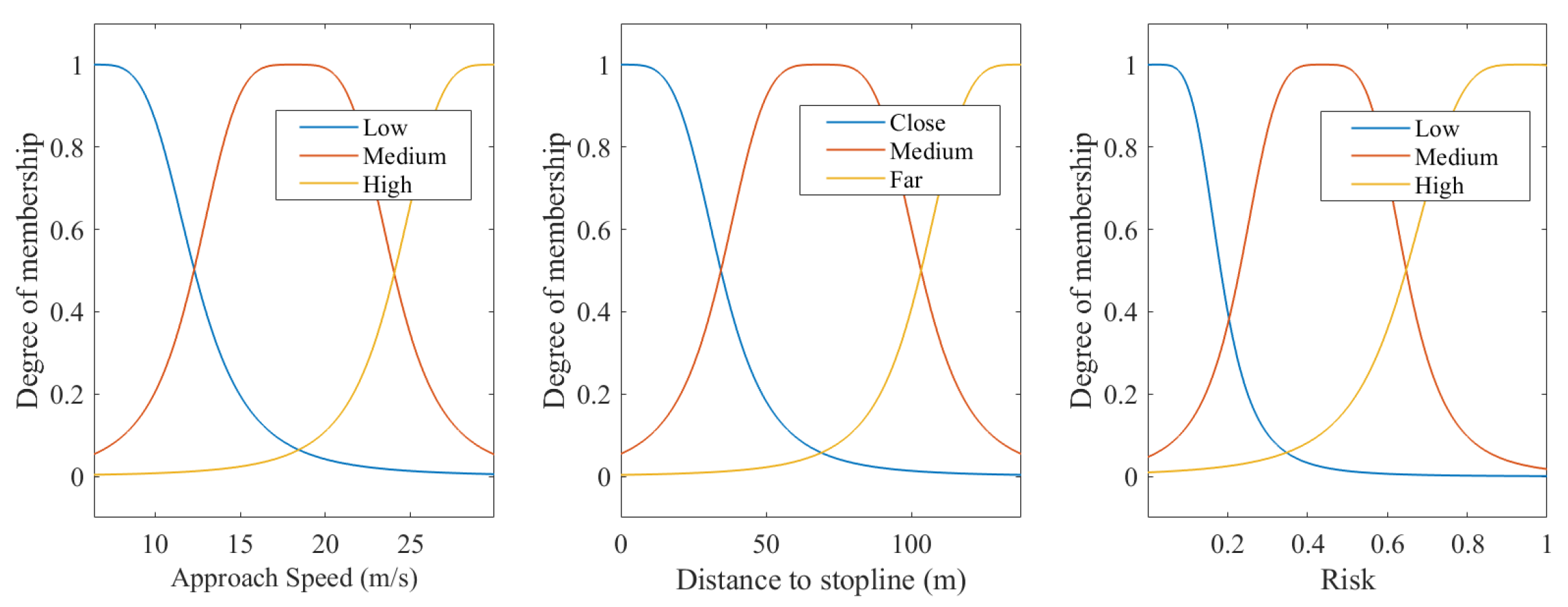
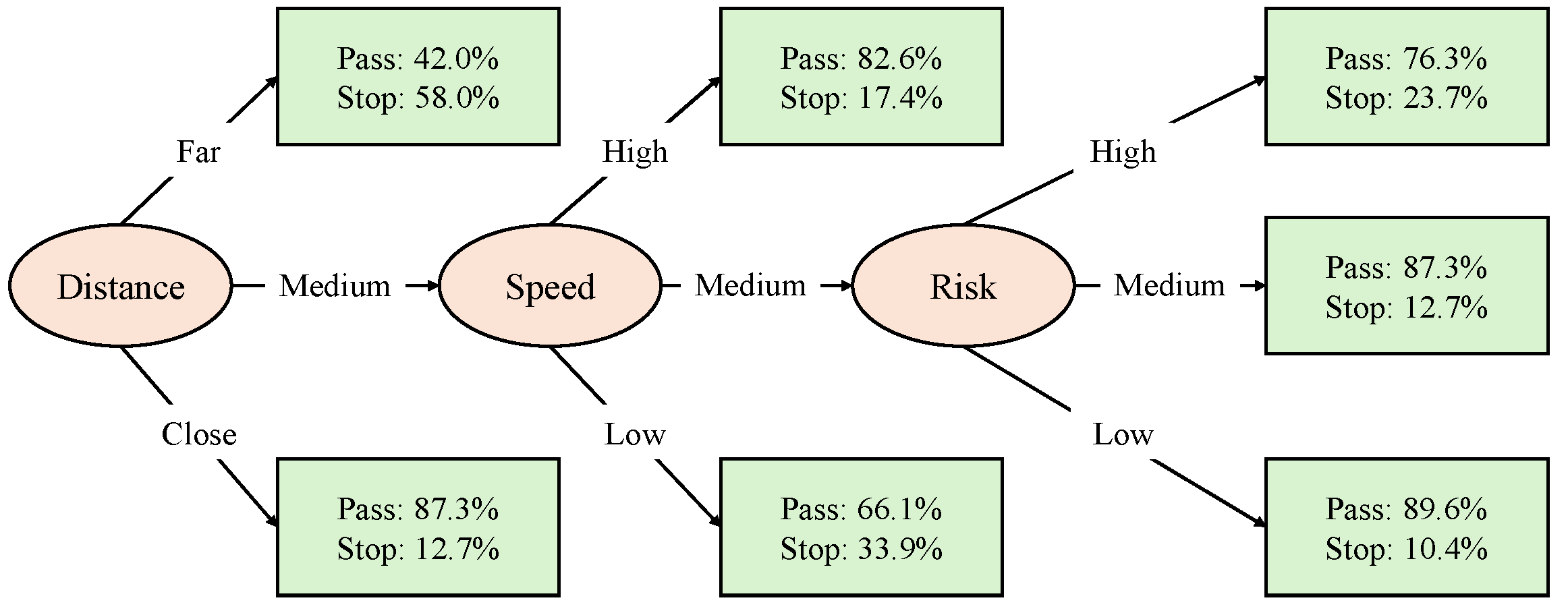
3.3. Fuzzy Decision
3.4. Motion Planning
4. Simulation Framework
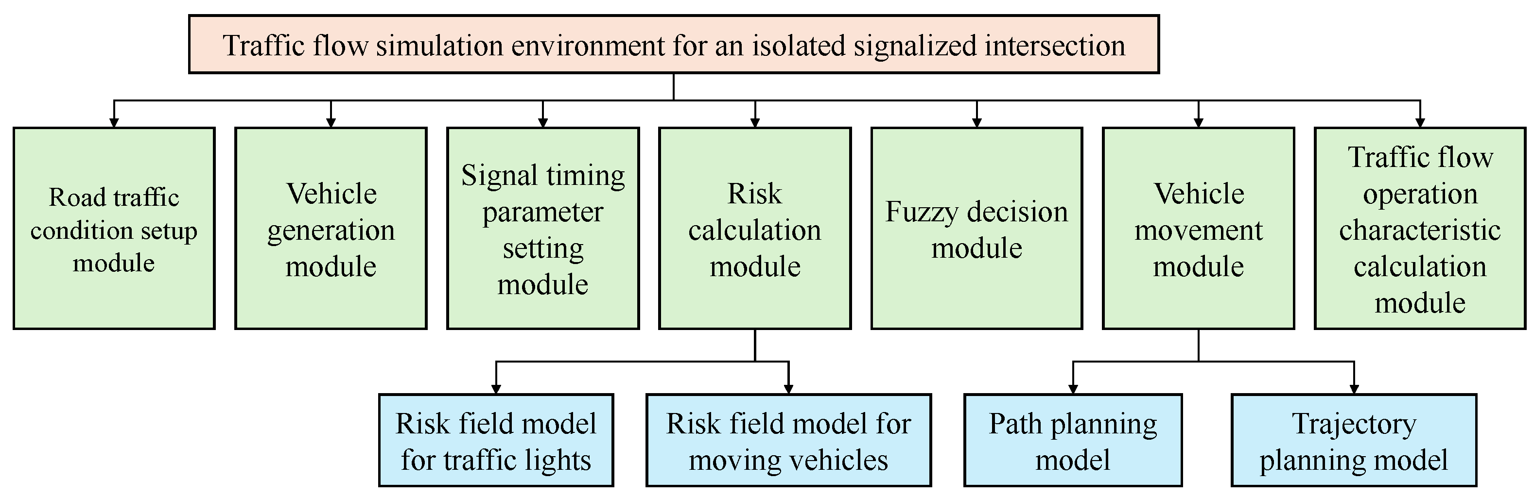
4.1. Building Simulation Environment
4.2. Setting Simulation Parameters
- The total length of the upstream segment of the signalized intersection is 2000 m.
- To intuitively analyze the traffic volume for each direction and specifically observe the impact of yellow phase duration, the approach direction was individually configured with three lanes, with vehicle departure proportions for left-turn, straight, and right-turn lanes set at 30%, 30%, and 40%, respectively, without considering lane-changing behavior on the upstream segment.
- It is assumed that vehicle departures follow a Poisson curve, with the number of departing vehicles per unit time (λ) set at 0.2 veh/s, 0.3 veh/s, and 0.4 veh/s. For all vehicles, the departure speed was set as equal to the intersection design speed.
- The simulation duration is 3600 s. The signal cycle length is 123 s, with a constant green duration, and three signal timing schemes are set:
- ✧
- Green light lasts for 60 s, yellow light lasts for 3 s, and red light lasts for 60 s.
- ✧
- Green light lasts for 60 s, yellow light lasts for 4 s, and red light lasts for 59 s.
- ✧
- Green light lasts for 60 s, yellow light lasts for 5 s, and red light lasts for 58 s.
- It is assumed that vehicles strictly adhere to the intersection design speed, meaning they always travel at the speed limit in a free-flowing state. Since the observed maximum acceleration rate is nearly 4 m/s2 and the maximum deceleration rate is about 8 m/s2, the range of vehicle acceleration is from −8 to 4 m/s2, and overtaking is not allowed during travel.
5. Results
5.1. Traffic Volume
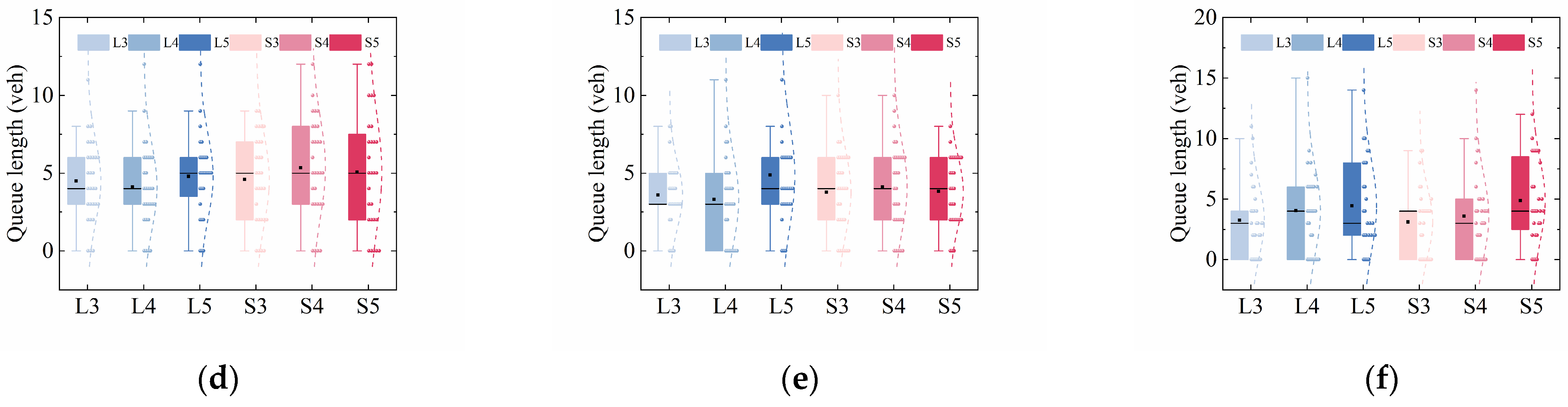
5.2. Queue Length
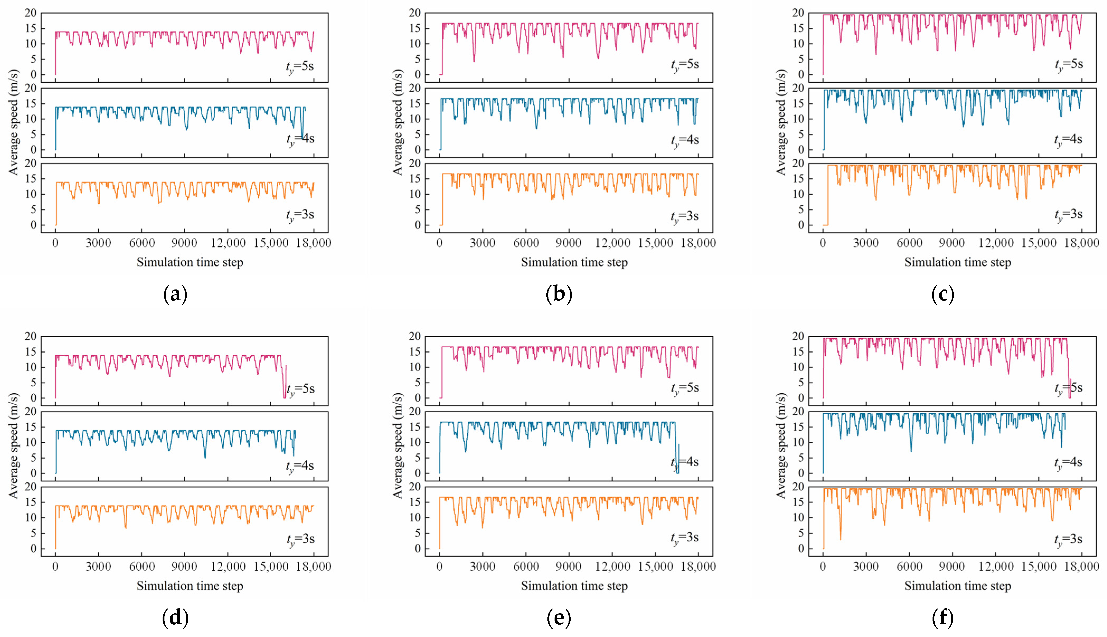
5.3. Average Speed
5.4. Safety
6. Discussion
6.1. Traffic Volume
6.2. Queue Length
6.3. Average Speed
6.4. Safety
7. Conclusions
Author Contributions
Funding
Data Availability Statement
Conflicts of Interest
References
- Banks, J. Principles of simulation. In Handbook of Simulation; Oxford University Press: Oxford, UK, 1998; Volume 12, pp. 3–30. [Google Scholar]
- Bossel, H. Modeling and Simulation; AK Peters: Natick, MA, USA; CRC Press: Boca Raton, FL, USA, 2018. [Google Scholar]
- Turner, B.L. Model laboratories: A quick-start guide for design of simulation experiments for dynamic systems models. Ecol. Model. 2020, 434, 109246. [Google Scholar] [CrossRef]
- Saidallah, M.; El Fergougui, A.; Elalaoui, A.E. A comparative study of urban road traffic simulators. In MATEC Web of Conferences; EDP Sciences: Les Ulis, France, 2016; Volume 81, p. 05002. [Google Scholar]
- Vrbanić, F.; Čakija, D.; Kušić, K.; Ivanjko, E. Traffic flow simulators with connected and autonomous vehicles: A short review. Transform. Transp. 2021, 15–30. [Google Scholar] [CrossRef]
- Silgu, M.A.; Erdağı, İ.G.; Göksu, G.; Celikoglu, H.B. Combined control of freeway traffic involving cooperative adaptive cruise controlled and human driven vehicles using feedback control through SUMO. IEEE Trans. Intell. Transp. Syst. 2021, 23, 11011–11025. [Google Scholar] [CrossRef]
- Wang, T.; Hussain, A.; Bhutta, M.N.M.; Cao, Y. Enabling bidirectional traffic mobility for ITS simulation in smart city environments. Future Gener. Comput. Syst. 2019, 92, 342–356. [Google Scholar] [CrossRef]
- Hua, J.; Lu, G.; Liu, H.X. Modeling and simulation of approaching behaviors to signalized intersections based on risk quantification. Transp. Res. Part C Emerg. Technol. 2022, 142, 103773. [Google Scholar] [CrossRef]
- Liu, P.; Zhao, J.; Zhang, F.; Yeo, H. Modeling decision-making process of drivers during yellow signal phase at intersections based on drift–diffusion model. Transp. Res. Part F Traffic Psychol. Behav. 2024, 105, 368–384. [Google Scholar] [CrossRef]
- Papadopoulos, E.; Nikolaidou, A.; Lilis, E.; Politis, I.; Papaioannou, P. Extending the decision-making process during yellow phase from human drivers to autonomous vehicles: A microsimulation study with safety considerations. J. Traffic Transp. Eng. (Engl. Ed.) 2024, 11, 362–379. [Google Scholar] [CrossRef]
- Tan, H.; Lu, G.; Liu, M. Risk field model of driving and its application in modeling car-following behavior. IEEE Trans. Intell. Transp. Syst. 2021, 23, 11605–11620. [Google Scholar] [CrossRef]
- Wang, Z.; Lu, G.; Tan, H.; Liu, M. A risk-field based motion planning method for multi-vehicle conflict scenario. IEEE Trans. Veh. Technol. 2023, 73, 310–322. [Google Scholar] [CrossRef]
- Wang, Z.; Lu, G.; Tan, H. Driving behavior model for multi-vehicle interaction at uncontrolled intersections based on risk field considering drivers’ visual field characteristics. IEEE Trans. Intell. Transp. Syst. 2024, 25, 15532–15546. [Google Scholar] [CrossRef]
- Tan, H.; Lu, G.; Wang, Z.; Hua, J.; Liu, M. A unified risk field-based driving behavior model for car-following and lane-changing behaviors simulation. Simul. Model. Pract. Theory 2024, 136, 102991. [Google Scholar] [CrossRef]
- Al-Turki, M.; Jamal, A.; Al-Ahmadi, H.M.; Al-Sughaiyer, M.A.; Zahid, M. On the potential impacts of smart traffic control for delay, fuel energy consumption, and emissions: An NSGA-II-based optimization case study from Dhahran, Saudi Arabia. Sustainability 2020, 12, 7394. [Google Scholar] [CrossRef]
- Qadri, S.S.S.M.; Gökçe, M.A.; Öner, E. State-of-art review of traffic signal control methods: Challenges and opportunities. Eur. Transp. Res. Rev. 2020, 12, 1–23. [Google Scholar] [CrossRef]
- Eom, M.; Kim, B.I. The traffic signal control problem for intersections: A review. Eur. Transp. Res. Rev. 2020, 12, 1–20. [Google Scholar] [CrossRef]
- Pawar, D.S.; Pathak, D.; Patil, G.R. Modeling dynamic distribution of dilemma zone at signalized intersections for developing world traffic. J. Transp. Saf. Secur. 2022, 14, 886–904. [Google Scholar] [CrossRef]
- Wu, Y.; Abdel-Aty, M.; Ding, Y.; Jia, B.; Shi, Q.; Yan, X. Comparison of proposed countermeasures for dilemma zone at signalized intersections based on cellular automata simulations. Accid. Anal. Prev. 2018, 116, 69–78. [Google Scholar] [CrossRef]
- Tang, K.; Xu, Y.; Wang, F.; Oguchi, T. Exploring stop-go decision zones at rural high-speed intersections with flashing green signal and insufficient yellow time in China. Accid. Anal. Prev. 2016, 95, 470–478. [Google Scholar] [CrossRef]
- Chen, C.; Chen, Y.; Ma, J.; Zhang, G.; Walton, C.M. Driver behavior formulation in intersection dilemma zones with phone use distraction via a logit-Bayesian network hybrid approach. J. Intell. Transp. Syst. 2018, 22, 311–324. [Google Scholar] [CrossRef]
- Kim, S.; Son, Y.J.; Chiu, Y.C.; Jeffers, M.A.B.; Yang, C.D. Impact of road environment on drivers’ behaviors in dilemma zone: Application of agent-based simulation. Accid. Anal. Prev. 2016, 96, 329–340. [Google Scholar] [CrossRef]
- Bao, J.; Chen, Q.; Luo, D.; Wu, Y.; Liang, Z. Exploring the impact of signal types and adjacent vehicles on drivers’ choices after the onset of yellow. Phys. A Stat. Mech. Its Appl. 2018, 500, 222–236. [Google Scholar] [CrossRef]
- Wolfgram, J. A Safety and Emissions Analysis of Continuous Flow Intersections. Master’s Thesis, University of Massachusetts Amherst, Amherst, MA, USA, 2018. [Google Scholar]
- Du, M.; Yang, S.; Chen, Q. Impacts of vehicle-to-infrastructure communication on traffic flows with mixed connected vehicles and human-driven vehicles. Int. J. Mod. Phys. B 2021, 35, 2150091. [Google Scholar] [CrossRef]
- Jiang, H.; Hu, J.; An, S.; Wang, M.; Park, B.B. Eco approaching at an isolated signalized intersection under partially connected and automated vehicles environment. Transp. Res. Part C Emerg. Technol. 2017, 79, 290–307. [Google Scholar] [CrossRef]
- Xiao, X.; Zhang, Y.; Wang, X.; Yang, S.; Chen, T. Hierarchical longitudinal control for connected and automated vehicles in mixed traffic on a signalized arterial. Sustainability 2021, 13, 8852. [Google Scholar] [CrossRef]
- Yao, H.; Li, X. Decentralized control of connected automated vehicle trajectories in mixed traffic at an isolated signalized intersection. Transp. Res. Part C Emerg. Technol. 2020, 121, 102846. [Google Scholar] [CrossRef]
- Yao, H.; Li, X. Lane-change-aware connected automated vehicle trajectory optimization at a signalized intersection with multi-lane roads. Transp. Res. Part C Emerg. Technol. 2021, 129, 103182. [Google Scholar] [CrossRef]
- Yu, M.; Long, J. An eco-driving strategy for partially connected automated vehicles at a signalized intersection. IEEE Trans. Intell. Transp. Syst. 2022, 23, 15780–15793. [Google Scholar] [CrossRef]
- Zhao, W.; Ngoduy, D.; Shepherd, S.; Liu, R.; Papageorgiou, M. A platoon based cooperative eco-driving model for mixed automated and human-driven vehicles at a signalised intersection. Transp. Res. Part C Emerg. Technol. 2018, 95, 802–821. [Google Scholar] [CrossRef]
- Chen, C.; Wang, J.; Xu, Q.; Wang, J.; Li, K. Mixed platoon control of automated and human-driven vehicles at a signalized intersection: Dynamical analysis and optimal control. Transp. Res. Part C Emerg. Technol. 2021, 127, 103138. [Google Scholar] [CrossRef]
- Ma, C.; Yu, C.; Yang, X. Trajectory planning for connected and automated vehicles at isolated signalized intersections under mixed traffic environment. Transp. Res. Part C Emerg. Technol. 2021, 130, 103309. [Google Scholar] [CrossRef]
- Cheng, Y.; Chen, C.; Hu, X.; Chen, K.; Tang, Q.; Song, Y. Enhancing mixed traffic flow safety via connected and autonomous vehicle trajectory planning with a reinforcement learning approach. J. Adv. Transp. 2021, 2021, 6117890. [Google Scholar] [CrossRef]
- Lin, D.; Yang, X.; Gao, C. VISSIM-based simulation analysis on road network of CBD in Beijing, China. Procedia-Soc. Behav. Sci. 2013, 96, 461–472. [Google Scholar] [CrossRef]
- Ma, X.; Jin, J.; Lei, W. Multi-criteria analysis of optimal signal plans using microscopic traffic models. Transp. Res. Part D Transp. Environ. 2014, 32, 1–14. [Google Scholar] [CrossRef]
- Paul, M.; Ghosh, I.; Haque, M.M. The effects of green signal countdown timer and retiming of signal intervals on dilemma zone related crash risk at signalized intersections under heterogeneous traffic conditions. Saf. Sci. 2022, 154, 105862. [Google Scholar] [CrossRef]
- Smith, D.; Djahel, S.; Murphy, J. A SUMO based evaluation of road incidents’ impact on traffic congestion level in smart cities. In Proceedings of the 39th Annual IEEE Conference on Local Computer Networks Workshops, Edmonton, AB, Canada, 8–11 September 2014; IEEE: Piscataway, NJ, USA, 2014; pp. 702–710. [Google Scholar]
- Flötteröd, Y.P.; Behrisch, M. Improving SUMO’s Signal Control Programs by Introducing Route Information. EPiC Ser. Eng. 2018, 2, 162–172. [Google Scholar]
- Zhang, Y.; Su, R. An optimization model and traffic light control scheme for heterogeneous traffic systems. Transp. Res. Part C Emerg. Technol. 2021, 124, 102911. [Google Scholar] [CrossRef]
- Varga, B.; Doba, D.; Tettamanti, T. Optimizing vehicle dynamics co-simulation performance by introducing mesoscopic traffic simulation. Simul. Model. Pract. Theory 2023, 125, 102739. [Google Scholar] [CrossRef]
- Ronaldo, A. Comparison of the Two Micro-Simulation Software Aimsun & Sumo for Highway Traffic Modelling. Master’s Thesis, Linköping University, Linköping, Sweden, 2012. [Google Scholar]
- Sun, B.; Appiah, J.; Park, B.B. Practical guidance for using mesoscopic simulation tools. Transp. Res. Procedia 2020, 48, 764–776. [Google Scholar] [CrossRef]
- Abedian, S.; Mirsanjari, M.M.; Salmanmahiny, A. Investigating the effect of suburban buses on traffic flow and carbon monoxide emission by Aimsun simulation software. J. Indian Soc. Remote Sens. 2021, 49, 1319–1330. [Google Scholar] [CrossRef]
- Ansariyar, A.; Taherpour, A. Investigating the accuracy rate of vehicle-vehicle conflicts by LIDAR technology and microsimulation in VISSIM and AIMSUN. Adv. Transp. Stud. 2023, 61, 37–52. [Google Scholar]
- Wang, Q.; Li, L.; Hou, D.; Li, Z.; Hu, J. Simulation study on the effect of automated driving in a road network environment. IET Intell. Transp. Syst. 2020, 14, 228–232. [Google Scholar] [CrossRef]
- Raju, N.; Farah, H. Evolution of traffic microsimulation and its use for modeling connected and automated vehicles. J. Adv. Transp. 2021, 2021, 2444363. [Google Scholar] [CrossRef]
- Coropulis, S.; Berloco, N.; Gentile, R.; Intini, P.; Ranieri, V. The use of microscopic simulators for safety assessment in automated and partially automated scenarios: A comparison. Transp. Res. Procedia 2023, 69, 313–320. [Google Scholar] [CrossRef]
- Sagaama, I.; Kchiche, A.; Trojet, W.; Kamoun, F. Energy consumption models in VANET simulation tools for electric vehicles: A literature survey. Int. J. Ad Hoc Ubiquitous Comput. 2023, 42, 30–46. [Google Scholar] [CrossRef]
- Laubenbacher, R.; Jarrah, A.S.; Mortveit, H.S.; Ravi, S.S. Agent-based modeling, mathematical formalism for. In Complex Social and Behavioral Systems: Game Theory and Agent-Based Models; Springer: Berlin/Heidelberg, Germany, 2020; pp. 683–703. [Google Scholar]
- Tzouras, P.G.; Mitropoulos, L.; Stavropoulou, E.; Antoniou, E.; Koliou, K.; Karolemeas, C.; Karaloulis, A.; Mitropoulos, K.; Tarousi, M.; Vlahogianni, E.I.; et al. Agent-based models for simulating e-scooter sharing services: A review and a qualitative assessment. Int. J. Transp. Sci. Technol. 2023, 12, 71–85. [Google Scholar] [CrossRef]
- Othman, N.B.; Jayaraman, V.; Chan, W.; Loh, Z.X.K.; Rajendram, R.; Mepparambath, R.M.; Agrawal, P.; Ramli, M.A.; Qin, Z. SUMMIT: A multi-modal agent-based co-simulation of urban public transport with applications in contingency planning. Simul. Model. Pract. Theory 2023, 126, 102760. [Google Scholar] [CrossRef]
- Gao, Z.; Guan, X.; Guo, K. Driver directional control model and the application in the research of intelligent vehicle. China J. Highw. Transp. 2000, 13, 106–109. [Google Scholar]
- Almadi, A.I.; Al Mamlook, R.E.; Almarhabi, Y.; Ullah, I.; Jamal, A.; Bandara, N. A fuzzy-logic approach based on driver decision-making behavior modeling and simulation. Sustainability 2022, 14, 8874. [Google Scholar] [CrossRef]
- Hurwitz, D.S.; Wang, H.; Knodler Jr, M.A.; Ni, D.; Moore, D. Fuzzy sets to describe driver behavior in the dilemma zone of high-speed signalized intersections. Transp. Res. Part F Traffic Psychol. Behav. 2012, 15, 132–143. [Google Scholar] [CrossRef]
- Yang, Z.; Tian, X.; Wang, W.; Zhou, X.; Liang, H. Research on driver behavior in yellow interval at signalized intersections. Math. Probl. Eng. 2014, 2014, 518782. [Google Scholar] [CrossRef]
- Lu, G.; Wang, Y.; Wu, X.; Liu, H.X. Analysis of yellow-light running at signalized intersections using high-resolution traffic data. Transp. Res. Part A Policy Pract. 2015, 73, 39–52. [Google Scholar] [CrossRef]
- Liu, H.X.; Wu, X.; Ma, W.; Hu, H. Real-time queue length estimation for congested signalized intersections. Transp. Res. Part C Emerg. Technol. 2009, 17, 412–427. [Google Scholar] [CrossRef]
- Lu, G.; Hua, J.; Zhao, H.; Liu, M.; Xu, J.; Zong, F. Modeling Vehicle Paths at Intersections: A Unified Approach Based on Entrance and Exit Lanes. IEEE Trans. Intell. Transp. Syst. 2023, 24, 14097–14110. [Google Scholar] [CrossRef]
- Wilde, G.J.S. The theory of risk homeostasis: Implications for safety and health. Risk Anal. 1982, 2, 209–225. [Google Scholar] [CrossRef]
- Hurwitz, D.; Abadi, M.G.; McCrea, S.; Quayle, S.; Marnell, P. Smart Red Clearance Extensions to Reduce Red-Light Running Crashes; No. FHWA-OR-RD-16-10; Oregon. Dept. of Transportation: Salem, OR, USA, 2016. [Google Scholar]
- Li, K. Guidelines for Traffic Signal Control—Current German Regulations (RiLSA); China Construction Industry Press: Shanghai, China, 2006. [Google Scholar]
- Li, K.; Yang, P.; Ni, Y. Amber interval design at urban signalized intersections. Urban Transp. China 2010, 8, 67–72. [Google Scholar]
- Chen, Y.; Kong, D.; Sun, L.; Zhang, T.; Song, Y. Fundamental diagram and stability analysis for heterogeneous traffic flow considering human-driven vehicle driver’s acceptance of cooperative adaptive cruise control vehicles. Phys. A Stat. Mech. Its Appl. 2022, 589, 126647. [Google Scholar] [CrossRef]
- Ma, J.; Xu, Y.; Ji, H.; Su, B. Multi-agent microsimulation of urban intersections considering yellow light driving behavior. J. Syst. Eng. 2015, 30, 394–405. [Google Scholar]
- Comert, G.; Khan, Z.; Rahman, M.; Chowdhury, M. Grey models for short-term queue length predictions for adaptive traffic signal control. Expert Syst. Appl. 2021, 185, 115618. [Google Scholar] [CrossRef]
- Chiou, Y.C.; Chang, C.H. Driver responses to green and red vehicular signal countdown displays: Safety and efficiency aspects. Accid. Anal. Prev. 2010, 42, 1057–1065. [Google Scholar] [CrossRef]
- Fayazi, S.A.; Vahidi, A. Mixed-integer linear programming for optimal scheduling of autonomous vehicle intersection crossing. IEEE Trans. Intell. Veh. 2018, 3, 287–299. [Google Scholar] [CrossRef]
- Kaul, R.; Jipp, M. Influence of cognitive processes on driver decision-making in dilemma zone. Transp. Res. Interdiscip. Perspect. 2023, 19, 100805. [Google Scholar] [CrossRef]
- Hoogendoorn, S.; Knoop, V. Traffic flow theory and modelling. In The Transport System and Transport Policy: An Introduction; Edward Elgar Publishing: Cheltenham, UK, 2013; pp. 125–159. [Google Scholar]
- Durrani, U.; Lee, C.; Shah, D. Predicting driver reaction time and deceleration: Comparison of perception-reaction thresholds and evidence accumulation framework. Accid. Anal. Prev. 2021, 149, 105889. [Google Scholar] [CrossRef] [PubMed]
- Adavikottu, A.; Velaga, N.R. Analysis of speed reductions and crash risk of aggressive drivers during emergent pre-crash scenarios at unsignalized intersections. Accid. Anal. Prev. 2023, 187, 107088. [Google Scholar] [CrossRef]
- El-Shawarby, I.; Rakha, H.; Inman, V.W.; Davis, G.W. Evaluation of driver deceleration behavior at signalized intersections. Transp. Res. Rec. 2007, 2018, 29–35. [Google Scholar] [CrossRef]
- Adavikottu, A.; Velaga, N.R.; Mishra, S. Modelling the effect of aggressive driver behavior on longitudinal performance measures during car-following. Transp. Res. Part F Traffic Psychol. Behav. 2023, 92, 176–200. [Google Scholar] [CrossRef]
- Sharma, A.; Zheng, Z.; Kim, J.; Bhaskar, A.; Haque, M.M. Assessing traffic disturbance, efficiency, and safety of the mixed traffic flow of connected vehicles and traditional vehicles by considering human factors. Transp. Res. Part C Emerg. Technol. 2021, 124, 102934. [Google Scholar] [CrossRef]
- Maiti, N.; Chilukuri, B.R. Does anisotropy hold in mixed traffic conditions? Phys. A Stat. Mech. Its Appl. 2023, 632, 129336. [Google Scholar] [CrossRef]
- Knoflacher, H. Der Einfluß des Grünblinkens auf die Leistungsfähigkeit und Sicherheit lichtsignalgeregelter Straßenkreuzungen. Strassenforschung 1973, 8, 1–4. [Google Scholar]
- Bonneson, J.A.; Zimmerman, K.H. Effect of yellow-interval timing on the frequency of red-light violations at urban intersections. Transp. Res. Rec. 2004, 1865, 20–27. [Google Scholar] [CrossRef]
- Prasetijo, J.; Musa, I.; Sulaiman, N.A.; Mustafa, M.A.; Putranto, L.S.; Hamid, N.B.; Siang Alvin John, L.M.; Abd Latif, M.F. Red-light running vehicles behaviour based on linear regression approach at traffic lights along Bakau Condong Road, Batu Pahat, Johor. Int. J. Road Saf. 2020, 1, 4–8. [Google Scholar]
- Papaioannou, P.; Papadopoulos, E.; Nikolaidou, A.; Politis, I.; Basbas, S.; Kountouri, E. Dilemma zone: Modeling drivers’ decision at signalized intersections against aggressiveness and other factors using uav technology. Safety 2021, 7, 11. [Google Scholar] [CrossRef]
- Ren, Y.; Wang, Y.; Wu, X.; Yu, G.; Ding, C. Influential factors of red-light running at signalized intersection and prediction using a rare events logistic regression model. Accid. Anal. Prev. 2016, 95, 266–273. [Google Scholar] [CrossRef] [PubMed]
- Zhang, Y.; Fu, C.; Hu, L. Yellow light dilemma zone researches: A review. J. Traffic Transp. Eng. (Engl. Ed.) 2014, 1, 338–352. [Google Scholar] [CrossRef]
- Palat, B.; Delhomme, P. A simulator study of factors influencing drivers’ behavior at traffic lights. Transp. Res. Part F Traffic Psychol. Behav. 2016, 37, 107–118. [Google Scholar] [CrossRef]
- Chen, P.; Yu, G.; Wu, X.; Ren, Y.; Li, Y. Estimation of red-light running frequency using high-resolution traffic and signal data. Accid. Anal. Prev. 2017, 102, 235–247. [Google Scholar] [CrossRef]


| Software | Car-Following Model | Lane-Changing Model | Yielding Model at Intersections |
|---|---|---|---|
| VISSIM [10,35,36,37] | Physio-psycho model | Rule-based discrete choice model | Decision tree and priority rule-based model |
| SUMO [31,38,39,40,41] | Krauss model | Krauss model | Default priority rule and custom traffic rule-based model |
| AIMSUN [42,43,44,45] | Gipps model | Dynamic decision-making model | Priority rule and signal control-based model |
| PARAMICS [46,47,48,49] | Gipps model and fuzzy logic-based model | Fuzzy logic-based dynamic model | Fuzzy logic and priority rule-based model |
| TRANSIMS [50,51,52] | Custom agent-based model | Custom strategy-based model | Custom Rule-based models |
| Speed Limit (km/h) | Recommended Yellow Light Duration (s) |
|---|---|
| 50 | 3 |
| 60 | 4 |
| 70 | 5 |
| Number of Groups | ty (s) | λ (veh/s) | Vmax (km/h) |
|---|---|---|---|
| 1 | 3 | 0.2, 0.3, or 0.4 | 60 |
| 2 | 4 | 0.2, 0.3, or 0.4 | 60 |
| 3 | 5 | 0.2, 0.3, or 0.4 | 60 |
| 4 | 3 | 0.3 | 50, 60, or 70 |
| 5 | 4 | 0.3 | 50, 60, or 70 |
| 6 | 5 | 0.3 | 50, 60, or 70 |
| ty (s) | λ (veh/s) | Traffic Volume (veh/h) | |
|---|---|---|---|
| Left-Turn Lane | Straight Lane | ||
| 3 | 0.2 | 172 | 212 |
| 0.3 | 250 | 318 | |
| 0.4 | 343 | 411 | |
| 4 | 0.2 | 178 | 216 |
| 0.3 | 239 | 313 | |
| 0.4 | 358 | 422 | |
| 5 | 0.2 | 201 | 199 |
| 0.3 | 282 | 294 | |
| 0.4 | 387 | 420 | |
| ty (s) | Vmax (km/h) | Traffic Volume (veh/h) | |
|---|---|---|---|
| Left-Turn Lane | Straight Lane | ||
| 3 | 50 | 301 | 319 |
| 60 | 250 | 318 | |
| 70 | 305 | 316 | |
| 4 | 50 | 275 | 305 |
| 60 | 239 | 313 | |
| 70 | 311 | 292 | |
| 5 | 50 | 316 | 295 |
| 60 | 282 | 294 | |
| 70 | 308 | 308 | |
| ty (s) | λ (veh/s) | Yellow-Running Vehicles (veh) | Red-Running Vehicles (veh) | Unsafe Driving Vehicles (veh) | |||
|---|---|---|---|---|---|---|---|
| Left-Turn Lane | Straight Lane | Left-Turn Lane | Straight Lane | Left-Turn Lane | Straight Lane | ||
| 3 | 0.2 | 2 | 2 | 4 | 2 | 6 | 4 |
| 0.3 | 6 | 2 | 1 | 3 | 7 | 5 | |
| 0.4 | 5 | 7 | 5 | 3 | 10 | 10 | |
| 4 | 0.2 | 2 | 1 | 1 | 1 | 3 | 2 |
| 0.3 | 0 | 2 | 1 | 2 | 1 | 4 | |
| 0.4 | 2 | 2 | 3 | 2 | 5 | 4 | |
| 5 | 0.2 | 1 | 1 | 4 | 6 | 5 | 7 |
| 0.3 | 2 | 0 | 4 | 2 | 6 | 2 | |
| 0.4 | 0 | 1 | 1 | 2 | 1 | 3 | |
| ty (s) | Vmax (km/h) | Yellow-Running Vehicles (veh) | Red-Running Vehicles (veh) | Unsafe Driving Vehicles (veh) | |||
|---|---|---|---|---|---|---|---|
| Left-Turn Lane | Straight Lane | Left-Turn Lane | Straight Lane | Left-Turn Lane | Straight Lane | ||
| 3 | 50 | 3 | 4 | 1 | 6 | 4 | 10 |
| 60 | 6 | 2 | 1 | 3 | 7 | 5 | |
| 70 | 3 | 2 | 3 | 6 | 6 | 8 | |
| 4 | 50 | 3 | 2 | 1 | 1 | 4 | 3 |
| 60 | 0 | 2 | 1 | 2 | 1 | 4 | |
| 70 | 4 | 4 | 7 | 7 | 11 | 11 | |
| 5 | 50 | 1 | 0 | 0 | 0 | 1 | 0 |
| 60 | 2 | 0 | 4 | 2 | 6 | 2 | |
| 70 | 4 | 3 | 3 | 1 | 7 | 4 | |
Disclaimer/Publisher’s Note: The statements, opinions and data contained in all publications are solely those of the individual author(s) and contributor(s) and not of MDPI and/or the editor(s). MDPI and/or the editor(s) disclaim responsibility for any injury to people or property resulting from any ideas, methods, instructions or products referred to in the content. |
© 2025 by the authors. Licensee MDPI, Basel, Switzerland. This article is an open access article distributed under the terms and conditions of the Creative Commons Attribution (CC BY) license (https://creativecommons.org/licenses/by/4.0/).
Share and Cite
Hua, J.; Li, B.; Li, P.; Zhang, W.; Li, Z. Exploring the Impacts of Yellow Light Duration on Intersection Performance Under Driving Behavior Uncertainty: A Risk Perception and Fuzzy Decision-Based Simulation Framework. Appl. Sci. 2025, 15, 5758. https://doi.org/10.3390/app15105758
Hua J, Li B, Li P, Zhang W, Li Z. Exploring the Impacts of Yellow Light Duration on Intersection Performance Under Driving Behavior Uncertainty: A Risk Perception and Fuzzy Decision-Based Simulation Framework. Applied Sciences. 2025; 15(10):5758. https://doi.org/10.3390/app15105758
Chicago/Turabian StyleHua, Jun, Bin Li, Pengcheng Li, Wei Zhang, and Zhenhua Li. 2025. "Exploring the Impacts of Yellow Light Duration on Intersection Performance Under Driving Behavior Uncertainty: A Risk Perception and Fuzzy Decision-Based Simulation Framework" Applied Sciences 15, no. 10: 5758. https://doi.org/10.3390/app15105758
APA StyleHua, J., Li, B., Li, P., Zhang, W., & Li, Z. (2025). Exploring the Impacts of Yellow Light Duration on Intersection Performance Under Driving Behavior Uncertainty: A Risk Perception and Fuzzy Decision-Based Simulation Framework. Applied Sciences, 15(10), 5758. https://doi.org/10.3390/app15105758