Adaptive Learning Approach for Human Activity Recognition Using Data from Smartphone Sensors

Abstract

Every day humans interact with smartphones that have embedded sensors that enable the tracking of changing physical activities of the device owner. However, several problems arise with the recognition of multiple activities (such as walking, sitting, running, and other) on smartphones. Firstly, most of the devices do not recognize some activities well, such as walking upstairs or downstairs. Secondly, recognition algorithms are embedded into smartphone software and are static, unless updated. In this case, a recognition algorithm must be re-trained with training data of a specific size. Thus, an adaptive (also known as, online or incremental) learning algorithm would be useful in this situation. In this work, an adaptive learning and classification algorithm based on hidden Markov models (HMMs) is applied to human activity recognition, and an architecture model for smartphones is proposed. To create a self-learning method, a technique that involves building an incremental algorithm in a maximal likelihood framework has been developed. The adaptive algorithms created enable fast self-learning of the model parameters without requiring the device to store data obtained from sensors. It also does not require sending gathered data to a server over the network for additional processing, making them autonomous and independent from outside systems. Experiments involving the modeling of various activities as separate HMMs with different numbers of states, as well as modeling several activities connected to one HMM, were performed. A public dataset called the Activity Recognition Dataset was considered for this study. To generalize the results, different performance metrics were used in the validation of the proposed algorithm.

1. Introduction

Many different healthcare and entertainment applications have been created, adapting human activity recognition in smartphones with embedded sensors. Activity recognition is especially relevant for fitness, running, and other sports. A lot of smartphone users track their activity and how long they are active, count their steps, calculate burnt calories, detect falls or posture, and much more. Various apps have been created for such purposes. Initially, several wearable sensors were used to identify various physical activities for the aforementioned applications. However, because smartphones contain a variety of sensors, research has moved to these types of devices in recent years [1,2,3,4,5,6,7]. Smartphones are useful for human activity recognition because they come with a combination of sensors, including accelerometers and magnetic field sensors, gyroscopes, magnetometers, GPSs, and so on. Recently, many researchers started using smartphones to explore human activity recognition and algorithms used for learning various human activities [8].

For example, experiments with human activity recognition using cell phone accelerometers were performed in ref. [3]. In the paper, the extracted features from accelerometers were used with the following classification techniques: Multilayer Perceptron, Simple Logistic, Random Forest, LMT, SVM, and LogitBoost. These techniques showed good recognition accuracy in relation to walking, jogging, standing, and sitting, whereas climbing upstairs and downstairs were poorly recognized. A survey in ref. [9] analyzed activity recognition with smartphone sensors such as an accelerometer, ambient temperature sensor, light sensor, magnetometer, proximity sensor, barometer, humidity sensor, gyroscope, etc. Several categories of activities were analyzed, including simple activities like walking, jogging, standing or sitting; more complex activities like taking buses, shopping, and driving a car; and other categories of activities such as living, working, and health-related activities. The authors listed the major, common challenges for activity recognition using mobile sensors: subject sensitivity, location sensitivity, activity complexity, energy and resource constraints, and insufficient training sets.

The secure client–server architecture proposed in ref. [10] allowed for the creation of a real-time human activity recognition system. A K-nearest neighbors (KNN) algorithm was used for activity recognition. Up to 100% of recognition accuracy for running and walking activities was achieved. Also, the overall accuracy of the model reached up to 95%. Deep learning is also used in various studies of activity recognition, such as ref. [11]. Deep learning models require a lot of available data and computing resources, which are not available for wearable devices. Moreover, these models are often trained offline, which cannot be executed in real-time.

A survey of using Hidden Markov models (HMMs) in human activity recognition was performed in ref. [12]. A continuous HMM and discrete HMM were proposed as a hierarchical probabilistic model to recognize a user’s activities in smartphones. A separate HMM was used to model a single activity. In ref. [13], the authors proposed a user adaptation technique to improve a human activity recognition system based on an HMM. Several different physical activities (walking, walking upstairs, walking downstairs, sitting, standing, and lying down) were modeled. As reported, the experimental results showed a significant error rate reduction.

Various recognition algorithms can be divided into three parts by the nature of learning patterns in data. The first type is offline algorithms, with the classifiers trained solely before starting to use them. The second type is adaptive learning (also referred as online) algorithms, which are trained in real-time with incoming data as they are being used [14,15]. The third type is semi-online algorithms, which are initially trained in a supervised manner and then used in simultaneous real-time self-supervised learning and classification. Such algorithms can be autonomous as they perform all calculations independently from other systems.

Numerous studies conducted in this field have analyzed sensor data gathered for offline activity recognition. They often use various software suites, such as MATLAB and WEKA, containing machine learning algorithms [3,15]. Smartphones are now capable of running recognition systems themselves as available resources like CPUs, memory, and batteries grow increasingly powerful. Therefore, activity recognition systems can now be implemented on these more powerful smartphones in a fully online learning mode [16,17]. Several studies have examined offline activity recognition in depth [18,19,20]. Another common issue increasingly faced in offline learning, which would be dealt with using adaptive learning algorithms, is insufficient data [9]. Training data may not match data collected by device sensors in a real environment. Insufficient data increases the variability of model prediction for a given data point or a value that tells us how the data is spread. This means that the model will fit the training data perfectly, but will stop working as soon as new data are fed into it. Adaptive learning algorithms can solve this problem by continuously using new data in training and prediction. Thus, it is relevant to develop self-learning algorithms that would autonomously adapt HAR recognition for each individual device using data received from the sensors of the trained device. It is natural to use incremental algorithms that only recalculate the parameters necessary for recognizing activities at each step, using only the information of the current step, and consuming limited computer resources, i.e., the complexity of the incremental algorithm becomes linear in terms of the sample size and the computer time consumed. However, incremental algorithms, created on the basis of most well-known machine learning algorithms, are not autonomous; their operation is related to training and exchanging data in the cloud [21,22,23,24]. It is necessary to emphasize that HAR recognition tools, devoted to massive implementation on smart mobile devices, should also meet the requirements of algorithmic simplicity and computational economy. In this paper, we propose to apply maximum likelihood methods to achieve the above goals, since they provide optimal, asymptotically unbiased, consistent, and normally distributed estimates, ensuring the highest entropy and minimum recognition error, obtained using simple statistics in the form of weighted sample means or covariances. A special computational technique is used, allowing us to adapt direct maximum likelihood algorithms into incremental ones. In this way, the recursive hidden Markov model (RHMM) is created as an adaptive learning method for activity recognition using data from smartphone sensors. The application of this algorithm allows for gathering new data from sensors and using them to adjust the model parameters in real-time. The recognition of a number of physical activities where motion sensors are used in the recognition process was analyzed.

2. Adaptive Activity Recognition

The proposed system for human activity recognition consists of the following components, representing data processing stages: data gathering, preprocessing, feature extraction, and training or classification [25,26]:

• Data gathering: A specified sampling rate is used for collecting sensor data from smartphones.
• Preprocessing: At this step, the gathered raw data are transformed in a useful and efficient format. Since the data can consist of many irrelevant and missing parts, data cleaning is conducted, followed by windowing or segmentation of the data [27].
• Feature extraction: From the segmented raw data, various data features are extracted. Several types of data feature extraction analyses, such as frequency analysis (e.g., Fourier Transform) or statistical analysis (e.g., moments: Mean, Std-Deviation, 3rd Moment, 4th Moment, etc.), of the available features can be applied to create new features [28].
• Training and classification:

  -

  Training: The classifiers in an activity recognition system must be trained before they can be used. Training is a step that calculates the model parameters further used in classification. Training can be conducted either offline on a desktop computer or online on a smartphone. If offline training is used, raw data of human activities is gathered, stored on a computer, and then used in training to obtain model parameters [29]. If training is performed online, the raw data are processed immediately without storing the on the device. The model parameters obtained during training are then used in the online recognition of human activities.

  -

  Classification: Human activities are classified using trained classifiers. Like in training, it can be performed either offline using a machine learning tool or online directly on the smartphone [29].

In the activity recognition process, classification is an essential part. Over the last few years, different types of classification algorithms have been implemented on smartphones such as support vector machines (SVMs), decision trees, K-nearest neighbors (KNN), fuzzy classification, and neural networks [11,30]. As previously mentioned, supervised learning can be used to train activity recognition models for smartphones in either an online or offline mode. In an online mode, the classifiers are trained on smartphones in real-time, whereas in an offline mode, the classifiers are trained beforehand, typically on a computer.

Likewise, there are two alternatives for using the trained model to perform classification—locally on the device (offline and real-time) or in the cloud (online). These options have a significant effect on speed, power, privacy, and cost [15]. For example, if the cloud is used to make a prediction, the application must be connected to the internet, whereas if the predictions are performed locally on the device, some hardware constraints must be met. In this case, a smartphone might not be able to perform any type of machine learning due to RAM and CPU limitations.

Performing classification directly on the device (in an offline mode) might be useful in cases where an application cannot rely on network connectivity. In this case, speed and reliability are the main advantages because all sensor data are processed and used in real-time predictions locally on the smartphone, without sending requests to the cloud online. However, in the case of a static offline trained model, it is challenging to update the training model once it is being used to make predictions. The model might become out-of-date over time and stop working exactly as expected. Subsequently, it must be re-trained with more or newer data and updated with the application which contains it. On the other hand, in the cloud, the model can be continuously updated. Thus, it will be unnecessary to update the application of human activity recognition. And in the case of re-training, the updated model will be available to all users [31].

The offline approach where only the classification is implemented on smartphones while the training is performed on desktop computers has been used in the majority of studies. The key reason is the reduced computational cost of training. Only a few studies used online training, in which classifiers could be trained in real-time on smartphones. However, the real-time classification occurs without subsequent real-time model adaptation.

Further, we propose a model for online human activity recognition.

2.1. Proposed System Architecture

Let us propose the system architecture based on the machine learning algorithm to classify activities using features extracted from gathered sensor data. Note, the inertial signals are recorded from sensors, such as an accelerometer (ACC), gyroscope (GYR), and magnetometer (MAG), extracting the required features from these signals. Lastly, the machine learning module (classifier) estimates model parameters from feature vectors sent to this module and identifies which class (state) the given signal belongs to.

Parts of this proposed architecture are discussed further in detail.

2.1.1. Sensor Data Gathering

Depending on the smartphone, various sensors provide the data for training and classification. An accelerometer, gyroscope, and magnetometer can be used to gather data [25].

2.1.2. Feature Extraction

After gathering the data, they need to be transformed so as to extract the features that would provide all of the necessary information to the machine learning algorithm.

It is necessary to transform the gathered data in order to extract features that include all the information needed by the machine learning algorithm. First, the sequences of inertial signal samples are divided into frames with overlapping and fixed-width sliding windows, calculating for each frame a feature vector, which is required in learning the internal characteristics of the inertial signals. These features are well-known statistics, namely, the mean, correlation, signal magnitude area (SMA), autoregression coefficients, and some more complex ones. These features, together with time domain signals, are selected according to prior work and importance analysis [25,28,32,33].

The time domain signals are as follows [33]:

• Three accelerometer signals (XYZ axis).
• Three jerk signals given by the accelerometer signal data.
• One magnitude signal index computed as the vector-length of the three previous original accelerometer signals.
• The jerk magnitude index computed as the vector-length of these jerk signals.

The features estimated from the time domain signals are as follows:

• Mean value, computed usually as the average of readings per axis, where N is the number of readings for each sensor: ${\displaystyle \frac{1}{N}}{\sum }_{i=1}^N{x}_i$.
• Median absolute deviation to evaluate the variation around the mean value, computed as (for each axis) ${\displaystyle \frac{1}{N}}{\sum }_{i=1}^N|x_i-\mu |$.
• Standard deviation, quantifying the variation of readings from the mean value: $\sqrt{{\displaystyle \frac{1}{N}}{\sum }_{i=1}^N{x}_i-\mu }$.
• Average Resultant Acceleration, computed as the average of vector-lengths of each reading: ${\displaystyle \frac{1}{N}}{\sum }_{i=1}^N\sqrt{x_i^2+y_i^2+z_i^2}$.
• Minimum and maximum in a frame.

• Inter-quartile range to measure the variability in a dataset.
• Energy measure computed as the average of squared samples in a frame.
• Signal magnitude area (SMA) computed through the normalized integral.

Frequency domain signals are as follows [33]:

• Three Fast Fourier transforms (FFTs) computed from three original accelerometer signals.
• Three FFTs computed from three jerk accelerometer signals.
• One FFT computed from a magnitude signal.
• One FFT computed from a jerk magnitude signal.

The features estimated from frequency domain signals (including similar features to those from the time domain) are as follows:

• Frequency component index with the largest magnitude.
• Weighted average of the frequency components.
• Skewness and Kurtosis of the frequency domain signal.
• Histogram, which is constructed in a standard manner, dividing the range of minimum–maximum values of each axis into a specified number of equal-sized intervals, equipped with frequencies of hitting to these intervals: ${\displaystyle \frac{1}{N}}{\sum }_{i=1}^N[(x_i\in b_j)\to 1,$$j=1...10]$.

2.1.3. Algorithm for Classification

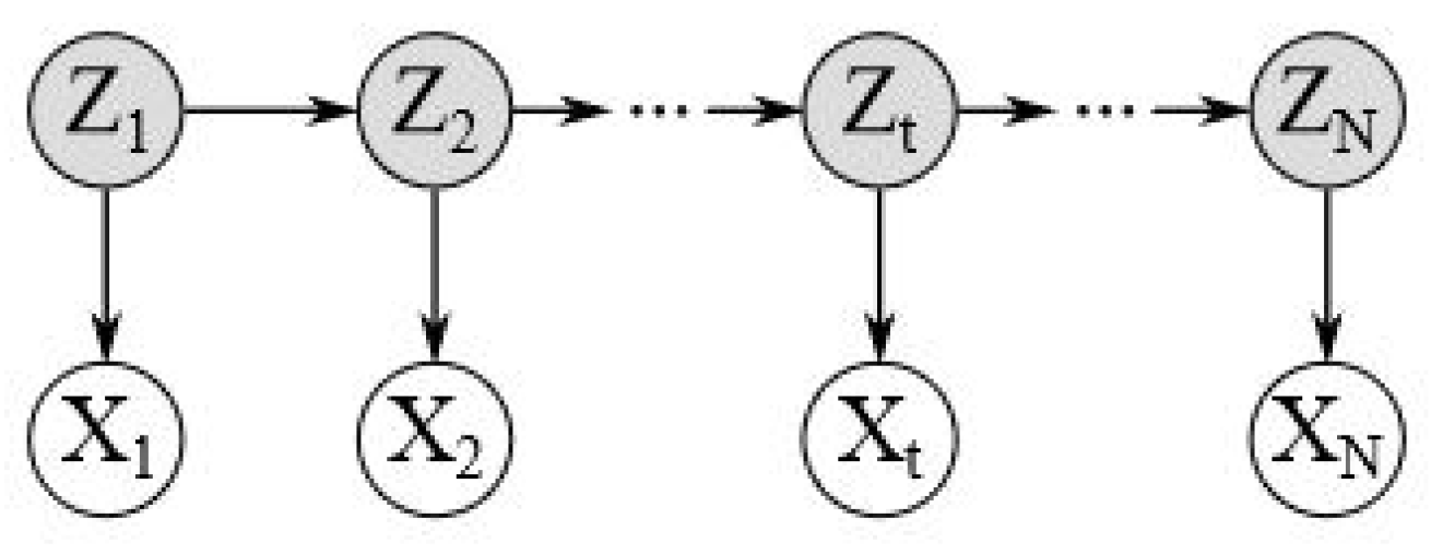
The recognition of human activities in a real-life setting is an important engineering and scientific problem. Several probability-based methods have been developed to build models to study it. HMM is a highly popular modeling technique for the analysis of stochastic processes by representing probability distributions over samples of observation, connected via Markov chains (Figure 1). In this model, an observation $X_t$ at time t is produced by a stochastic process in a certain state, although the state is considered as hidden. Thus, this hidden process is assumed to satisfy the Markov property, namely, state $Z_t$ at time t depends only on the previous state, $Z_{t-1}$ at time $t-1$. Hidden Markov model parameters that are estimated with observations are used in further analysis.

The Expectation–Maximization algorithm can be used to learn HMM parameters (emission probabilities B and transition probabilities), given the observation sequence and the set of the possible states in the HMM. The EM algorithm allows for iterative learning of HMM parameters. It computes the initial estimate of the parameters, and then uses these estimates to compute an improved estimate of the parameters. The EM algorithm is performed in the following steps: calculation of the logarithmic likelihood function and maximization of the conditional mean of the likelihood function. It is well known that the maximum likelihood estimate for an HMM is a consistent and asymptotically normal estimator, and it converges to a stationary point of the sample likelihood.

Various human activities can be modeled accurately as Markov chains [21,22,23,24,34,35]. Observing signals stemming from complex or unfamiliar activities can be utilized to indirectly build an HMM of the activity. There are two main ways an activity can be modeled with an HMM. The first one is to model one activity as a separate HMM. If it is denoted that one activity (for example, running) has a start, middle, and end, then this activity can be modeled with a minimum three-state HMM. The second one is to model several activities as one HMM. For example, if it is denoted that three activities (walking, running, and standing) are interconnected, and there are various possibilities to transition from one activity to another, then these activities can be modeled with one HMM. In this case, one state in HMM will represent one particular activity.

Similar to the above-mentioned classification, HMM parameters can be estimated in batch or online mode as well, where the online estimation algorithm allows for real-time sequential and re-evaluative parameter estimation. The model parameters are re-estimated on feed and processing with each new observation vector, without preserving previous observations data.

In this paper, an RHMM parameter estimation algorithm is proposed for HAR using the likelihood maximization and maximum likelihood estimates with sequential refinement of HMM parameters in an online setting [36].

Let us consider an HMM of N states with a sequence of observations of length T. Assume the HMM is stationary, i.e., its probabilistic properties do not change over time. Thus, denote the HMM state probability N-dimensional vector as $\gamma$; the state transition probability matrix as Q; and the density function of the probability distribution of observation o, generated from state s, as

$$\begin{array}{c}\hfill b({\mu }_s,{\sigma }_s)={\displaystyle \frac{1}{\sqrt{{\left(2\pi \right)}^n\left|{\sigma }_s\right|}}}{e}^{-{\displaystyle \frac{1}{2}}{(o-{\mu }_s)}^T{\sigma }_s^{-1}(o-{\mu }_s)},\end{array}$$

(1)

which is assumed to be normal with M-dimensional mean ${\mu }_s$ and covariance matrix ${\sigma }_s$ and $1\le s\le N$.

The logarithmic likelihood function, which describes the observation in a state s, is as follows:

$$\begin{array}{c}\hfill l(o,\mu ,\sigma )=-{\displaystyle \frac{n}{2}}ln\left(2\pi \right)-{\displaystyle \frac{1}{2}}ln\left(\right|\sigma \left|\right)-{\displaystyle \frac{1}{2}}{(o-\mu )}^T{\sigma }^{-1}(o-\mu ).\end{array}$$

(2)

Now one can define

$$\begin{array}{c}\hfill L(o,\mu ,\sigma ,\gamma )=\sum _{i=1}^N{e}^{-l(o,{\mu }_i,{\sigma }_i)+ln\left({\gamma }_i\right)}\end{array}$$

(3)

Let us calculate $lnL$ derivatives according to $\mu$, $\sigma$, and $\gamma$ using the Lagrange multiplier method regarding the constraint ${\sum }_{i=1}^N{\gamma }_i=1$:

$$\begin{array}{c}\hfill {\left(lnL\right)}_{{\mu }_i}^{\prime }={\varphi }_t^i\left(o-{\mu }_i\right){\sigma }_i^{-1},\end{array}$$

(4)

$$\begin{array}{c}\hfill {\left(lnL\right)}_{{\sigma }_i}^{\prime }={\varphi }_t^i\left({\sigma }_i^{-1}(o-{\mu }_i){(o-{\mu }_i)}^T{\sigma }_i^{-1}-{\sigma }_i^{-1}\right),\end{array}$$

(5)

$$\begin{array}{c}\hfill {\left(lnL+\lambda \left(1-\sum _{i=1}^N{\gamma }_i\right)\right)}_{{\gamma }_i}^{\prime }={\displaystyle \frac{{\varphi }_t^i}{{\gamma }_i}}-\lambda ,\end{array}$$

(6)

where ${\varphi }_t^i={\displaystyle \frac{e^{-l(o_t,\widehat{{\mu }_i},\widehat{{\sigma }_i})+ln\left({\gamma }_i\right)}}{{\sum }_{i=1}^N{e}^{-l(o_t,\widehat{{\mu }_i},\widehat{{\sigma }_i})+ln\left({\gamma }_i\right)}}}$, and $\lambda$ is the Lagrange multiplier.

The equations with derivatives ${\sum }_t{\left(lnL\right)}_{\mu }^{\prime }=0$, ${\sum }_t{\left(lnL\right)}_{\sigma }^{\prime }=0$, and ${\sum }_t{\left(lnL+\lambda \left(1-{\sum }_{i=1}^N{\gamma }_i\right)\right)}_{{\gamma }_i}^{\prime }$$=0$ are solved with respect to $\mu$, $\sigma$ and $\gamma$ as follows:

$$\begin{array}{c}\hfill \widehat{{\mu }_i}={\displaystyle \frac{{\sum }_{t=1}^T{\varphi }_t^i{o}_t}{{\sum }_{t=1}^T{\varphi }_t^i}},\end{array}$$

(7)

$$\begin{array}{c}\hfill \widehat{{\sigma }_i}={\displaystyle \frac{{\sum }_{t=1}^T{\varphi }_t^i(o_t-\widehat{{\mu }_i}){(o_t-\widehat{{\mu }_i})}^T}{{\sum }_{t=1}^T{\varphi }_t^i}},\end{array}$$

(8)

$$\begin{array}{c}\hfill {\gamma }_i={\displaystyle \frac{1}{T}}\sum _{t=1}^T{\varphi }_t^i.\end{array}$$

(9)

The derived Formulas (7) and (8) can be used in offline MLE estimation, given a fixed data sample. The complexity of such calculations is linear. However, if applied for online estimation, their complexity becomes of second order because the calculations must be carried out over the entire dataset at each appearance of new data (i.e., each re-estimation of parameters). Therefore, in order to enable online estimation, recursive formulas for re-estimating the HMM parameters are needed.

It is not difficult to observe that the estimates obtained by Formulas (7) and (8) at $t-1$ and t satisfy the following recursive relations:

$$\begin{array}{c}\hfill {\mu }_t^i={\mu }_{t-1}^i+{\displaystyle \frac{(o_t-{\mu }_{t-1}^i)}{t}}·{\displaystyle \frac{{\varphi }_t^i}{{\gamma }_t}},\end{array}$$

(10)

$$\begin{array}{c}\hfill {\sigma }_t^i={\displaystyle \frac{{\gamma }_{t-1}^i·(t-1)}{{\gamma }_t^i·t}}\left({\sigma }_{t-1}^i+{\displaystyle \frac{(o_t-{\mu }_{t-1}^i){(o_t-{\mu }_{t-1}^i)}^T}{t}}·{\displaystyle \frac{{\varphi }_t^i}{{\gamma }_t}}\right),\end{array}$$

(11)

where the state probabilities ${\gamma }_t^i={\displaystyle \frac{1}{t}}{\sum }_{i=1}^t{\varphi }_t^i$ are calculated as

$$\begin{array}{c}\hfill {\gamma }_t^i={\gamma }_{t-1}^i+{\displaystyle \frac{1}{t}}({\varphi }_t^i-{\gamma }_{t-1}^i).\end{array}$$

(12)

There are two parts of the RHMM parameter estimation algorithm.

The first part uses Equations (10)–(12) to estimate initial parameters given a small fixed-size observation set. During the initial training process, $\widehat{\mu }$ and $\widehat{\sigma }$ represent fixed parameter values used in estimation. The algorithm’s stability is ensured by initial training. However, usually, it is not difficult to have a large enough dataset to initialize parameter values that correctly identify and classify the observations. This crucial size is about 100–200; moreover, the proposed online algorithm is easily adapted for offline estimation. The second part uses Equations (10)–(12) to re-estimate parameters based on classified observations. The values of the previous steps $\widehat{\mu }$ and $\widehat{\sigma }$ are denoted by ${\mu }_{t-1}^i$ and ${\sigma }_{t-1}^i$ in the re-estimation process. A Bayes classifier is used to classify the observations into groups.

The proposed algorithm will be applied to human activity recognition. In this scenario, data from sensors are used to train and initialize the HMM model. Then, the trained model will be used for continuous activity recognition and real-time model parameter updating.

3. Results and Discussion

3.1. Dataset

The Activity Recognition System Dataset [37], which contains various measurements extracted from the sensors—accelerometers, gyroscopes, and magnetometers—have been used in our experiments:

• The acceleration in the X, Y, and Z axes measured by the sensor;
• The angular velocity in the X, Y, and Z axes measured by the sensor;
• The magnetic field in the X, Y, and Z axes measured by the sensor;
• The time extracted from the sensor in seconds.

The HAR System dataset, annotated manually by an observer, was compiled from data collected from 6 female and 10 male subjects aged between 23 and 50 [37]. One Inertial Measurement Unit (IMU), which provides data on the acceleration, magnetic field, and the turn rates in three dimensions, were mounted on the belt of the user. In total, it contains about 4.5 h of annotated activities: walking, walking upstairs, walking downstairs, running, standing, sitting, lying on the floor, falling, jumping forward, jumping backward, and jumping vertically [37].

3.2. Experimental Setup

In this section, we validate the performance of the RHMM parameter estimation algorithm using the Activity Recognition System Dataset. Firstly, feature extraction was performed (no other additional preprocessing was conducted on the data). Observation vectors of 28 dimensions were extracted for the experiments from the dataset using a window size of 30 milliseconds with a 50% overlap. The features extracted from the dataset for each activity were

• A mean value of accelerometer signals XYZ;
• Root mean square XYZ of accelerometer signals XYZ;
• Standard deviation XYZ of accelerometer signals XYZ;
• Signal vector magnitude of accelerometer signals;
• Signal magnitude area (FFT calculated from magnitude signal).

The following activities—modeled with a separate HMM state—were chosen for modeling and recognition: walking, walking upstairs, walking downstairs, running, standing, lying on the floor, sitting, and falling.

The online algorithm, using a fixed-size set of training observations, was implemented for initial HMM parameter evaluation, starting with randomly chosen initial parameters of mean and covariance.

The accuracy of the algorithm was explored using ten-fold cross-validation. In this procedure, the data were randomly sorted and divided into 10 folds and 10 rounds of cross-validation were run. In each round, one of the folds for validation was used, and the remaining folds were used for training. After training the model, its accuracy on the validation data was measured, and a final cross-validation accuracy was computed by obtaining the average accuracy over the 10 rounds.

3.3. Computational Details

The RHMM algorithm was implemented in Matlab. The performance of the algorithm was evaluated using accuracy, precision, recall, and F1-score because these metrics help us to notice and evaluate many recognition effects.

Accuracy, defined in Equation (13), presents itself simply as a ratio of correctly predicted observation to the total observations. This ratio is the most intuitive measure and tells us how often we can expect our machine learning model will correctly predict an outcome out of the total number of times it made predictions.

$$Accuracy=(TP+TN)/(TP+TN+FP+FN),$$

(13)

where TP, FP, TN, and FN represent the number of true positives, false positives, true negatives, and false negatives, respectively.

Recall, precision, and F1-score metrics were chosen in addition to the accuracy metric because they are useful measures of the success of prediction when the classes are imbalanced.

Recall, defined in Equation (14), enables us to indicate the model’s ability to correctly predict positive outcomes from true positive outcomes and is a good measure of successful prediction when classes are highly unbalanced.

$$Recall=TP/(TP+FN).$$

(14)

Precision, defined in Equation (15), is also a useful measure of successful prediction when classes are unbalanced.

$$Precision=TP/(TP+FP).$$

(15)

F1-score, defined in Equation (16), gives us equal weight to both precision and recall models when evaluating performance in terms of accuracy. In this way, it can be the alternative for accuracy metrics without knowing the total number of observations.

$$\mathit{\text{F1-score}}=2\left(Sp\dot{S}n\right)/(Sp+Sn).$$

(16)

3.4. Experiments

The first experiment was performed by modeling activities with separate HMMs consisting of varying amounts of states. The online algorithm was implemented as described above. Several cases of HMM modeling capabilities with different state amounts were analyzed. Five different models were trained with the proposed algorithm—three-state, four-state, five-state, six-state, and seven-state HMM models. Recognition accuracy was calculated during the continuous model parameter re-estimation and recognition.

In the first case of the three-state HMM, the accuracy of the model was 89%. Increasing the number of HMM states to four increased the accuracy to 91%. The accuracy stayed at 91% when the number of states was set to five. In the case of a six-state HMM, the accuracy reached 92%, whereas in the case of a seven-state HMM, it was 92%.

The results of these experiments show that increasing the state count from three to seven increases classification accuracy. For a better understanding of the performance of these models, the F1-score was calculated for each activity (see

Table 1. F1-score of each activity modeled with three- to seven-state HMM. The highest F1-score of each activity is in bold.

	3 States	4 States	5 States	6 States	7 States
Running	0.91	0.89	0.91	0.91	0.94
Walking	0.19	0.20	0.22	0.26	0.30
Walking upstairs	0.61	0.68	0.76	0.76	0.74
Walking downstairs	0.56	0.59	0.60	0.64	0.67
Standing	0.61	0.76	0.76	0.78	0.78
Sitting	0.18	0.24	0.24	0.25	0.26
Laying on the floor	0.90	0.75	0.71	0.67	0.65
Falling	0.92	0.96	0.89	0.93	0.93

). It gives some insight into how many states are needed to model HMM for the best recognition of each activity. Table 1 shows that running, walking, walking downstairs, and sitting activities have the best F1-score when they are modeled with seven-state HMM. Standing has the highest F1-score (0.78) when it is modeled with the seven- or six-state HMM. Walking upstairs modeled with five- or six-state HMM has the best F1-score. Laying on the floor modeled with the three-state HMM has the best F1-score of 0.9. It is a significant difference compared to the F1-score (0.65) of seven-state HMM. Falling has the highest F1-score (0.96) when this activity is modeled with four states. This experiment showed that different activities should not be modeled with the HMM of the same number of states if we want to achieve the best recognition results.

The confusion matrix of the experiments where each activity is modeled with the seven-state HMM is given in

Table 2. Confusion matrix for proposed algorithm where each activity is modeled as separate seven-state HMM.

		Predicted a
		R	W	WU	WD	ST	SI	L	F
Actual a	Run	80	0	0	0	0	0	0	5
	W	0	40	35	75	0	0	0	0
	WU	0	30	200	20	0	0	0	5
	WD	5	20	50	175	0	0	0	5
	ST	0	25	0	0	870	465	0	0
	SI	0	0	0	0	0	90	10	0
	L	0	0	0	0	0	40	50	5
	F	0	5	0	0	0	0	0	175

^a R = Running, W = Walking, WU = Walking upstairs; WD = Walking downstairs, ST = Standing, SI = Sitting, L = Laying, F = Falling.

. It shows that running, sitting, and falling are well discriminated among other activities. However, walking, walking upstairs, and walking downstairs are often confused with each other. Other static activities such as standing and lying are confused with each other as well.

Table 3. Performance metrics for each activity.

		Precision	Recall	F1-Score	Accuracy
Activity	Running	0.94	0.94	0.94	1.00
	Walking	0.27	0.33	0.30	0.92
	Walking upstairs	0.78	0.70	0.74	0.94
	Walking downstairs	0.69	0.65	0.67	0.93
	Standing	0.64	1.00	0.78	0.80
	Sitting	0.90	0.15	0.26	0.79
	Laying on the floor	0.53	0.83	0.65	0.98
	Falling	0.97	0.90	0.93	0.99
	Overall	0.68	0.68	0.68	0.92

shows the detailed algorithm performance metrics for each activity. Running, sitting, and falling reached the best precision out of all activities. The worst precision result occurred for the sitting activity. The best recall results were reached for running, standing, and fall activities. The worst recall and F1-score results occurred for walking and sitting activities.

The overall performance of the algorithm is presented in the last row of Table 3. It shows that the percentage error rate is 8% and the percentage success rate is 92%. While the accuracy of the algorithm is relatively high, precision, recall, and F1-score reached 0.68.

Further experiments were performed with the RHMM algorithm to analyze the recognition rate of activities in a case where all activities are modeled with a single HMM, e.g., one state of HMM represents one activity. Six different activities—standing, sitting, laying, walking, walking downstairs, walking upstairs—were chosen for this experiment. Laying on the floor and falling activities were left out because of the insufficient number of observations in the dataset. The confusion matrix of the proposed method was calculated (see

Table 4. Confusion matrix of activities for the proposed method where each activity is modeled as a single state of HMM.

		Predicted a
		ST	SI	L	W	WD	WU
Actual a	ST	98	0	2	0	0	0
	SI	20	70	10	0	0	0
	L	13	8	79	0	0	0
	W	0	0	0	77	18	6
	WD	0	0	0	3	87	10
	WU	0	1	1	4	2	92

^a W = Walking, WU = Walking upstairs; WD = Walking downstairs, ST = Standing, SI = Sitting, L = Laying.

).

Table 4 shows that more than 90% of standing and walking upstairs instances were correctly recognized. Walking downstairs was correctly recognized 80%. Laying and walking are above 70%, whereas sitting activity has the lowest recognition rate among all activities, at 69%. Further study showed that sitting and laying are often confused. The same applies for standing and sitting. However, activities of standing, sitting, and laying are well discriminated from walking, walking downstairs, and walking upstairs.

The computational time needed for the first and the second part of the algorithm to process one observation vector in the five-state HMM model was collected. The first part of the algorithm performs initial model training, whereas the second part performs recognition and parameter re-estimation. Experiments were conducted on Matlab with an Acer computer with Intel(R) Core(TM) i7-9750H CPU @ 2.60 GHz 2.59 GHz processor and 16.0 GB RAM. Computational time (in seconds) is given in

Table 5. Computational time in seconds.

	4D	10D	15D
First part	0.00296	0.00301	0.00306
Second part	0.07131	0.07009	0.07260

. It shows the computational time’s dependency on dimensions of observation. We can see that there is a small increase (around 1 millisecond) in computational time when dimensions of observation increase. Secondly, it is obvious that the second part of the algorithm is taking more time to process the observation than the first part because not only does it re-estimate the model parameters, but it also classifies the observation to one of the activities.

The proposed online activity recognition system is adaptable because it would allow users to train the system in real-time to meet their specific needs. It is important because different users may walk, run, or climb differently than others. The same behavior cannot be applied by generalizing it to all users because models trained offline are dependent on users on whom the training data were collected as well as tested. It can have an impact on how well the system can recognize human activities in real-life situations. This problem can be solved by the proposed online algorithm, which adapts to new situations.

For future research, we propose making a resource consumption analysis like CPU, memory, and battery usage, for an algorithm implemented in a smartphone. It is significant because the proposed algorithm does not merely make a classification on-the-fly but is also updating model parameters. It would be a key factor in deciding whether or not this algorithm could be implemented on smartphones.

It is apparent that confusion between some activities results in lower performance metrics. The experiments of activity modeling with four- to seven-state HMMs showed that a bigger state number resulted in a higher recognition rate. It might be useful to research modeling different activities with a different number of states because simple activities might need fewer state numbers than more complex ones.

4. Conclusions

This paper presents an application of the online algorithm to human activity recognition using data from smartphone sensors. The goal is to create an efficient algorithm that is optimal in terms of computer resource usage in a certain class of models, autonomous and algorithmically simple, with the aim of adapting it to mass use by smart device users. For this goal, the maximum likelihood method is applied using our developed technique for building the incremental algorithm. The architecture for activity recognition was proposed, where a fixed amount of data from sensors is used for initial model parameter approximation. Then, it uses a self-supervised learning, incremental method to recognize activities and update model parameters with each new observation received. The computer-based experiments show that for online data analysis, the online algorithm reaches a recognition accuracy of 92%. The performance of individual activities modeled with an HMM of a different number of states is studied as well. It showed that different activities should be modeled with a specific number of states in HMM. The proposed online activity recognition algorithm supports user personalization so that users can train a system online according to their needs.