Abstract
Photovoltaic (PV) systems are key renewable energy sources due to their ease of implementation, scalability, and global solar availability. Enhancing their lifespan and performance is vital for wider adoption. Identifying degradation root causes is essential for improving PV design and maintenance, thus extending lifespan. This paper proposes a hybrid fault diagnosis method combining a bond graph-based PV cell model with empirical degradation models to simulate faults, and a deep learning approach for root-cause detection. The experimentally validated model simulates degradation effects on measurable variables (voltage, current, ambient, and cell temperatures). The resulting dataset trains an Optimized Feed-Forward Neural Network (OFFNN), achieving 75.43% accuracy in multi-class classification, which effectively identifies degradation processes.
1. Introduction
The identification of degradation root causes in photovoltaic (PV) cells is critical for improving design efficiency and optimizing maintenance by targeting specific degradation mechanisms, thus reducing time and cost. However, developing such approaches faces challenges: limited instrumentation (typically voltage, current, ambient, and cell temperature sensors) and incomplete datasets, often restricted to normal operation with sparse faulty data [1,2,3].
Recent reviews [3,4] highlight that data-driven methods, particularly artificial intelligence-based techniques, excel in fault detection, achieving over 90% accuracy when comprehensive datasets are available [4]. Common targets include electrical faults (e.g., short circuits) addressed by shallow neural networks and visible faults (e.g., shading) by deep neural networks like Multi-layer Perceptrons and Convolutional Neural Networks [4]. Multivariate techniques, such as Principal Component Analysis (PCA) with Support Vector Machines (SVM), also succeed in detecting partial shading and disconnections [5]. Yet, real-world datasets often lack coverage of material-level degradation (e.g., Light Induced Degradation (LID), micro-cracks), limiting diagnostic scope.
To address this, empirical models of degradation phenomena—e.g., LID [6], Potential Induced Degradation (PID) [7], micro-cracks [8], corrosion [9], and Ethylene-Vinyl Acetate (EVA) discoloration [10]—have been developed from lab data. These models, while representative, are rarely used online due to their disconnect from measurable variables.
The identification of degradation mechanisms in PV systems has therefore gained renewed interest, especially with the advancement of digital twin frameworks and intelligent fault detection techniques. However, most existing solutions rely heavily on either black-box data-driven models that lack interpretability or overly simplified physical models that cannot fully capture real-world fault complexity. Notable efforts to analyze degradation mechanisms include studies by Logerais et al. [9], Braisaz et al. [11], and Papargyri and Paggi [12], though these often target specific faults in isolation rather than providing a generalizable solution.
In this paper, we propose a reproducible and modular methodology that integrates physical modeling with empirical degradation behaviors and machine learning-based classification. A generic PV cell simulator is developed using bond graph methodology [13], capturing electro-thermal dynamics and supporting degradation embedding. This enables the generation of synthetic, labeled datasets under varied fault conditions. An optimized Feed-Forward Neural Network (OFFNN) is trained on this dataset, using ReliefF feature selection [14] to identify the most informative inputs. This hybrid simulation–classification framework promotes scalability, interpretability, and open reproducibility, aligning with recent developments in smart energy management and automation in PV systems [15].
2. Modeling and Degradation Simulation
The proposed model serves as a simulator to generate degraded operation data beyond real-world datasets. Built using bond graph methodology—a multi-physical tool with causal and structural properties [13]—it adapts to various PV cell and panel sizes. Parameters have explicit physical meaning, enabling integration of empirical degradation models (detailed in Appendix B). A summary of bond graph elements is in Appendix A.
2.1. Elementary Cell Model
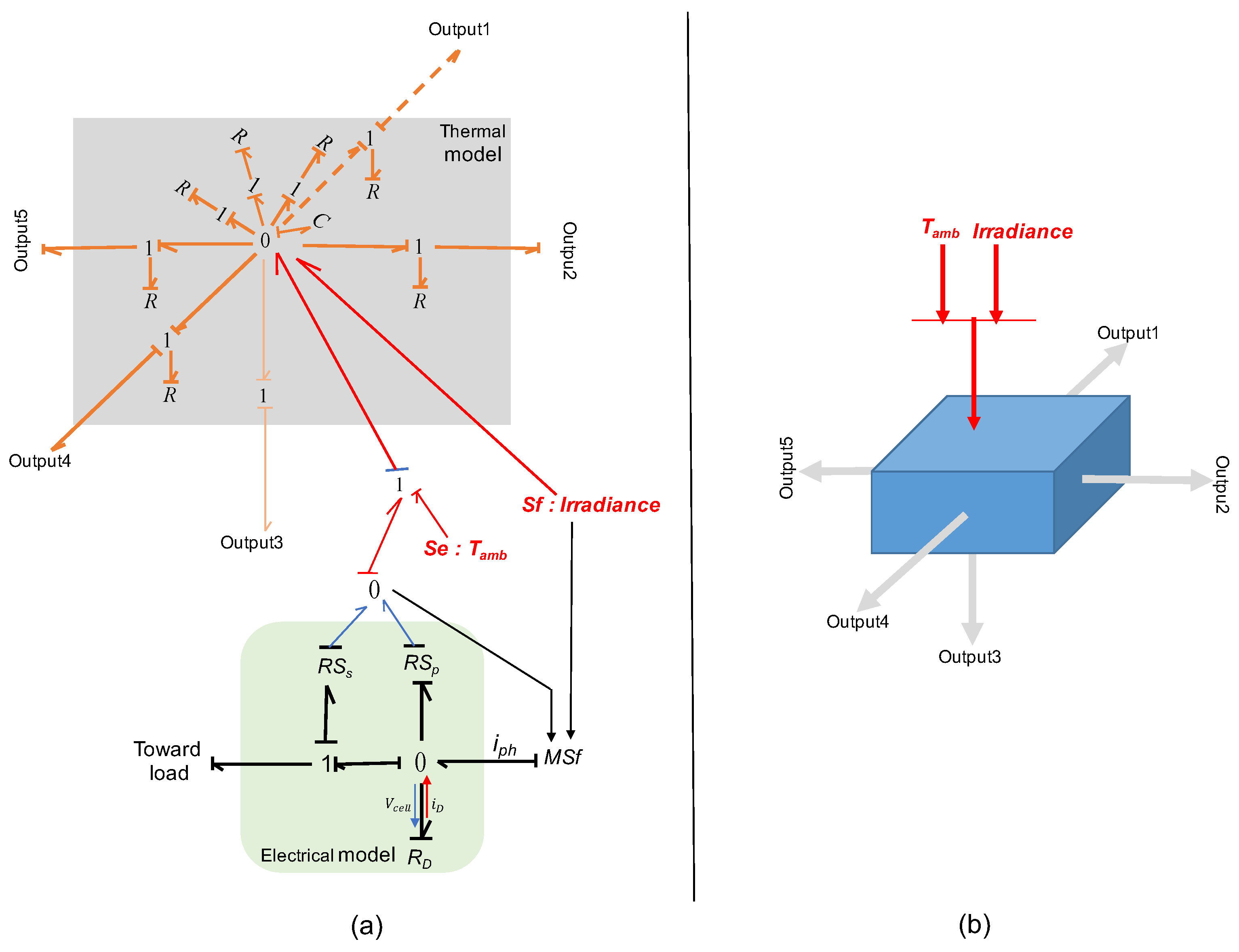
The PV cell model comprises interacting thermal and electro-thermal components. The thermal model assumes uniform heating from irradiance and electrical activity, using R-elements () for heat distribution and a C-element for volume, defined by material properties (specific heat c, density ) and dimensions (). The electro-thermal model (Figure 1), validated against one-diode models [16], includes a diode (), parallel resistor (), and series resistor (), with thermal effects via RS-elements. Cell current is , where reflects irradiance and temperature effects (see Appendix B for equations).
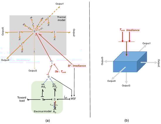
Figure 1.
Schematic representation of an elementary photovoltaic cell model. (a) The bond graph illustrates thermal and electro-thermal interactions within the cell. (b) The equivalent block diagram summarizes the key system components for simulation and analysis.
Figure 2 illustrates panel construction by connecting cells, adaptable to any size, supporting scalable fault diagnosis.
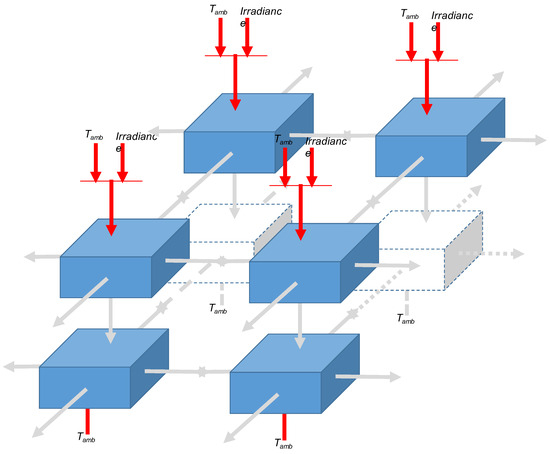
Figure 2.
Diagram showing how elementary PV cells are interconnected to form a full photovoltaic panel. This modular structure enables scalability and fault simulation across various panel sizes.
2.2. Model Validation
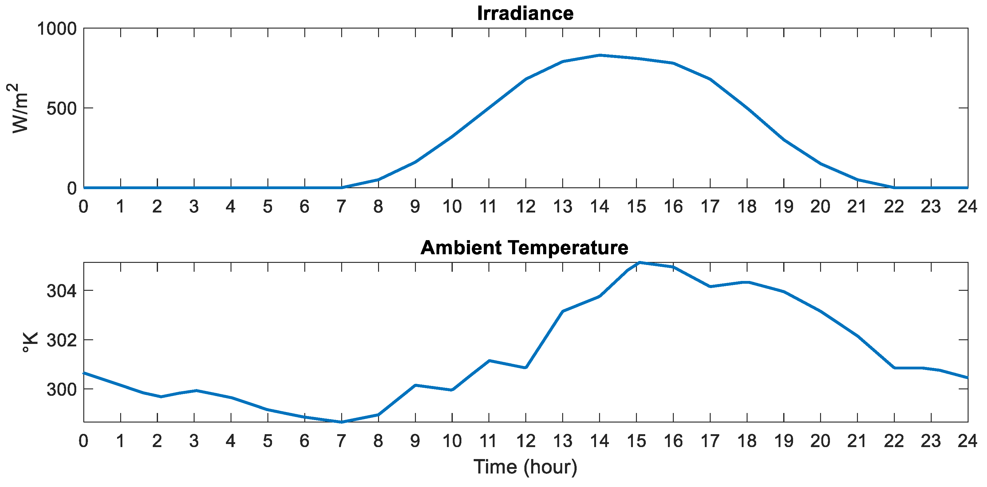
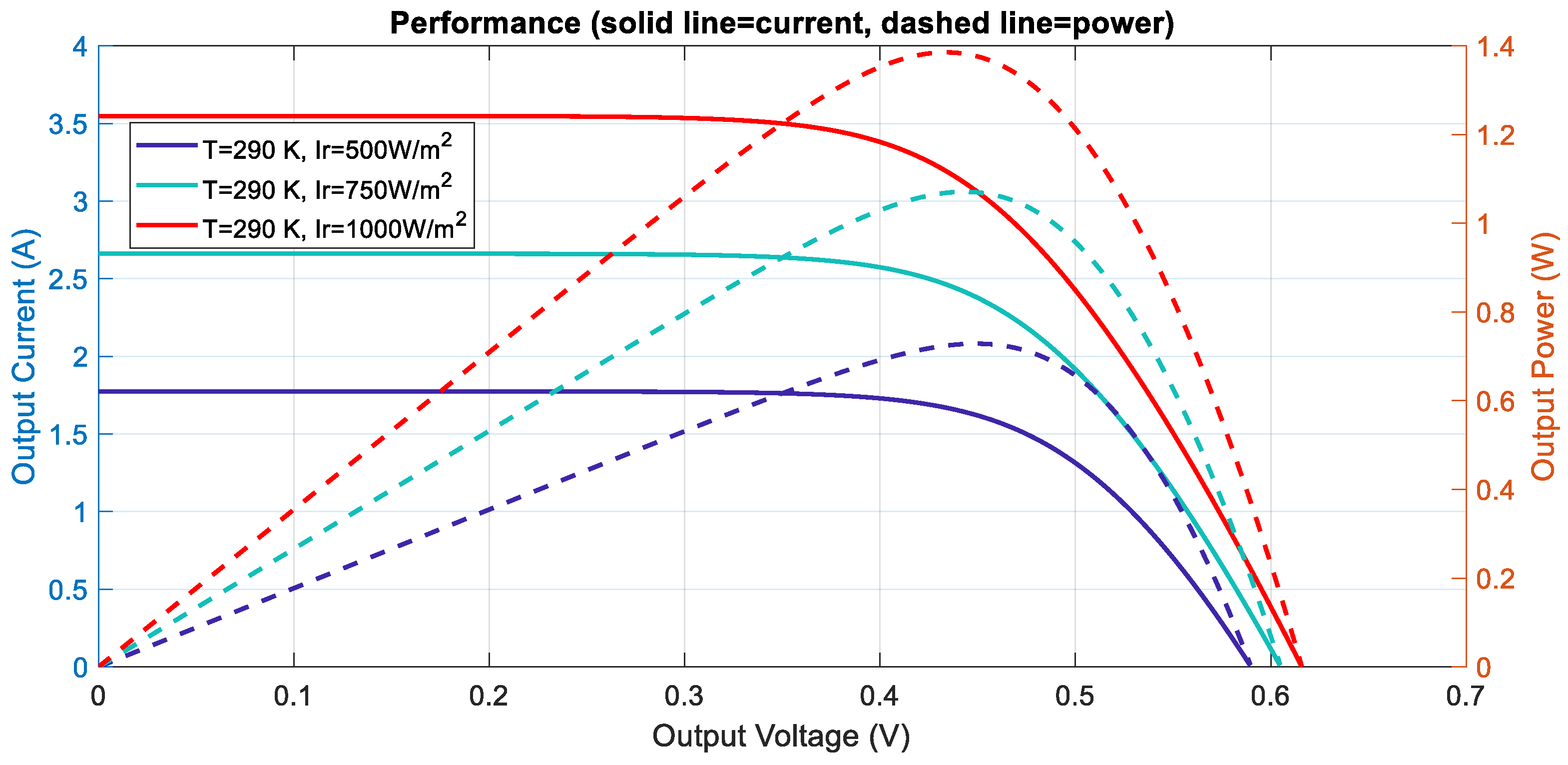
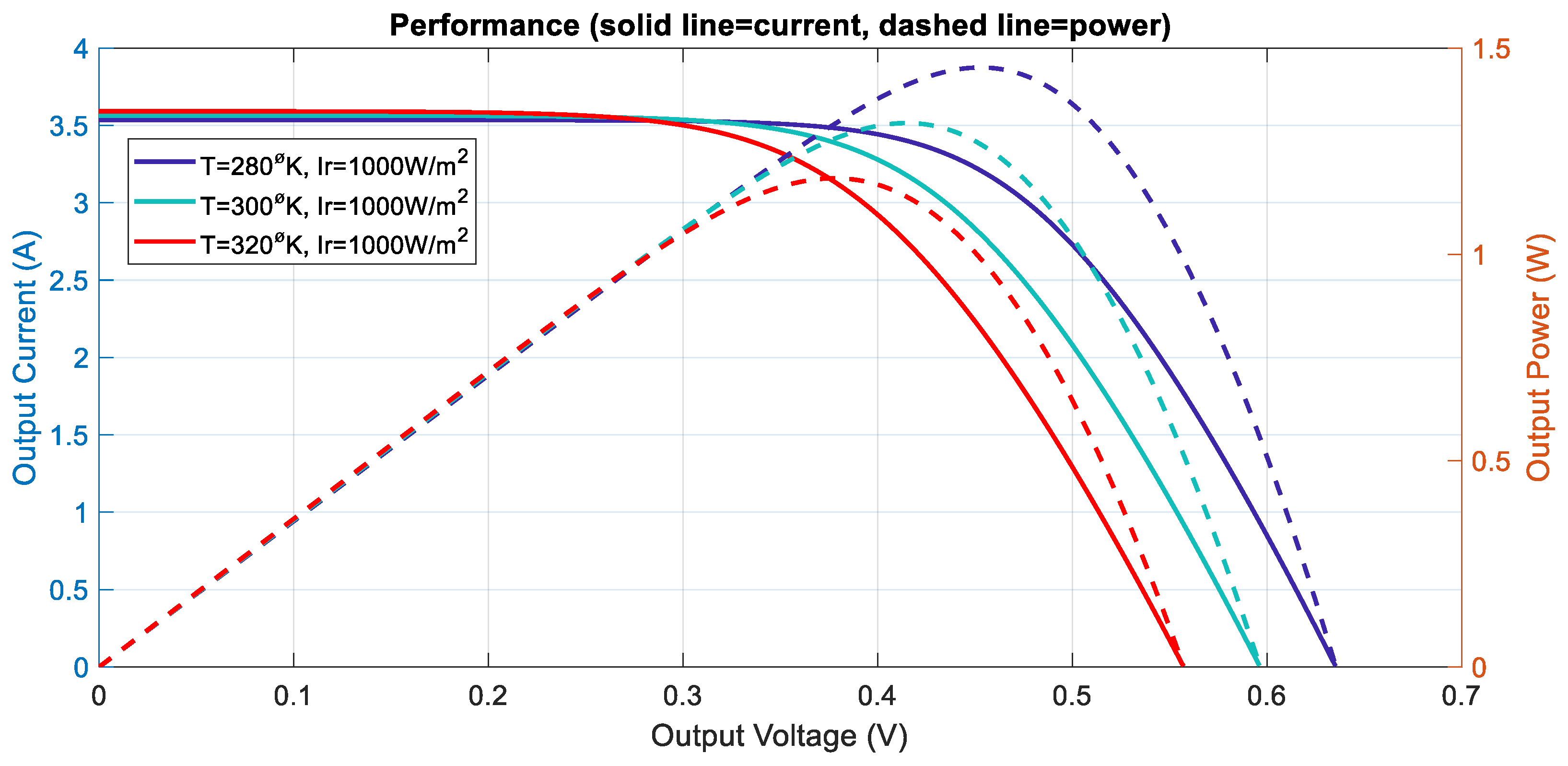
Using real 24-h data [17] (Figure 3), simulations confirm power proportionality to irradiance (Figure 4) and inverse proportionality to temperature (Figure 5), aligning with [18,19]. While our validation is based on synthetic data aligned with known physical behaviors, future improvements could involve hardware-in-the-loop setups for more realistic validation [20].
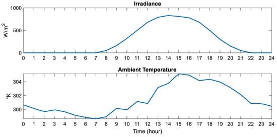
Figure 3.
Twenty-four-hour environmental data (irradiance and ambient temperature) recorded on 15 July 2011, used to validate model behavior under realistic solar exposure conditions.
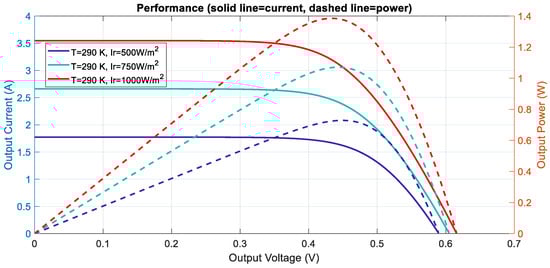
Figure 4.
Relationship between irradiance levels and PV power output, confirming the expected linear increase in generated power with irradiance at constant temperature.
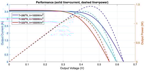
Figure 5.
Power output of the PV system under different cell temperatures, illustrating the inverse relationship between temperature and efficiency at fixed irradiance.
2.3. Degradation Models
Five degradation phenomena—ageing, EVA discoloration, LID, cracking, and corrosion—are integrated into the simulator by adjusting , , and based on empirical models from [6,9,10,11,12,21,22]. Potential Induced Degradation (PID) was also considered, as it represents a major field-observed degradation mechanism. While full PID simulation is not implemented in the current version due to limited access to robust empirical models, its effects—typically manifested as a rapid drop in shunt resistance and/or increased leakage current across module insulation—are well documented [7]. To support future integration, a theoretical formulation has been included in Appendix B. Table 1 summarizes the associated degradation effects.

Table 1.
Summary of degradation effects.
Recent reviews [23] have comprehensively summarized the root causes and detection challenges associated with PV degradation, highlighting the need for integrated diagnostic frameworks similar to the one proposed in this work.
2.4. Simulation Assumptions and Reproducibility
To ensure reproducibility and transparency, the simulations were performed using a modular PV cell model based on bond graph methodology. The physical parameters used in the model—such as thermal capacitance, resistive losses, and current–voltage behavior—were selected based on standard datasheets for crystalline silicon PV cells and kept constant throughout all simulations. Each degradation mode was introduced by altering relevant parameters in the model, following established physical or empirical degradation mechanisms. For example, ageing effects on and were modeled according to [9], EVA discoloration was parameterized using the discoloration index defined in [10], and LID was modeled as an increase in photocurrent in line with [6]. Cracking-related leakage and current changes were modeled based on [12,21,22], while corrosion effects on series resistance followed the formulations in [11]. A theoretical outline for PID based on [7] is also included for future implementation.
The simulation workflow involved varying environmental conditions, including multiple irradiance levels, ambient temperatures, and aging stages. Fault scenarios were independently simulated to isolate the behavior of each degradation mechanism. All simulations followed a uniform structure to generate time-series outputs (voltage, current, and temperature), which were post-processed to extract statistical and physically interpretable features.
The neural network was trained on the resulting labeled dataset generated from these simulations. Although the precise implementation details (e.g., simulation step size, solver type, or software toolchain) are not the primary focus of this study, the overall methodology is modular and adaptable.
3. Root-Cause Detection and Identification Algorithm
The PV cell is equipped with voltage, current, ambient temperature, and cell temperature sensors. Normal operation data are real measurements, while degraded data are simulated (Section 2) across five classes: normal operation, EVA discoloration, cracks, LID, and Rsh wear (dust accumulation excluded due to bias [24]). The dataset comprises 75,000 samples (15,000 per class), generated under varying conditions (e.g., irradiance 0–1000 W/m2, temperature 280–320 K).
3.1. Classification Pipeline
Figure 6 outlines the classification process: sensor data are preprocessed, features selected via ReliefF, and classified using an Optimized Feed-Forward Neural Network (OFFNN) with a moving window approach [25].

Figure 6.
Workflow of the root-cause classification pipeline. Raw sensor data are preprocessed, with relevant features selected via ReliefF, and fed into an optimized feed-forward neural network (OFFNN) for degradation mode identification.
The core of the proposed approach lies in its hybrid structure, which integrates physical simulation with data-driven classification. A bond graph-based physical model is used to simulate time-series sensor data under various degradation scenarios by modifying parameters such as shunt resistance, series resistance, and photocurrent. These simulations are carried out across a range of environmental conditions to mimic realistic operational diversity. The resulting synthetic signals serve as labeled inputs to the machine learning stage. Specifically, the data are preprocessed, normalized, and used to train the OFFNN classifier. This simulation-to-classification pipeline enables effective root-cause detection, even in the absence of large-scale real-world fault datasets, and leverages the strengths of both physics-based interpretability and data-driven adaptability.
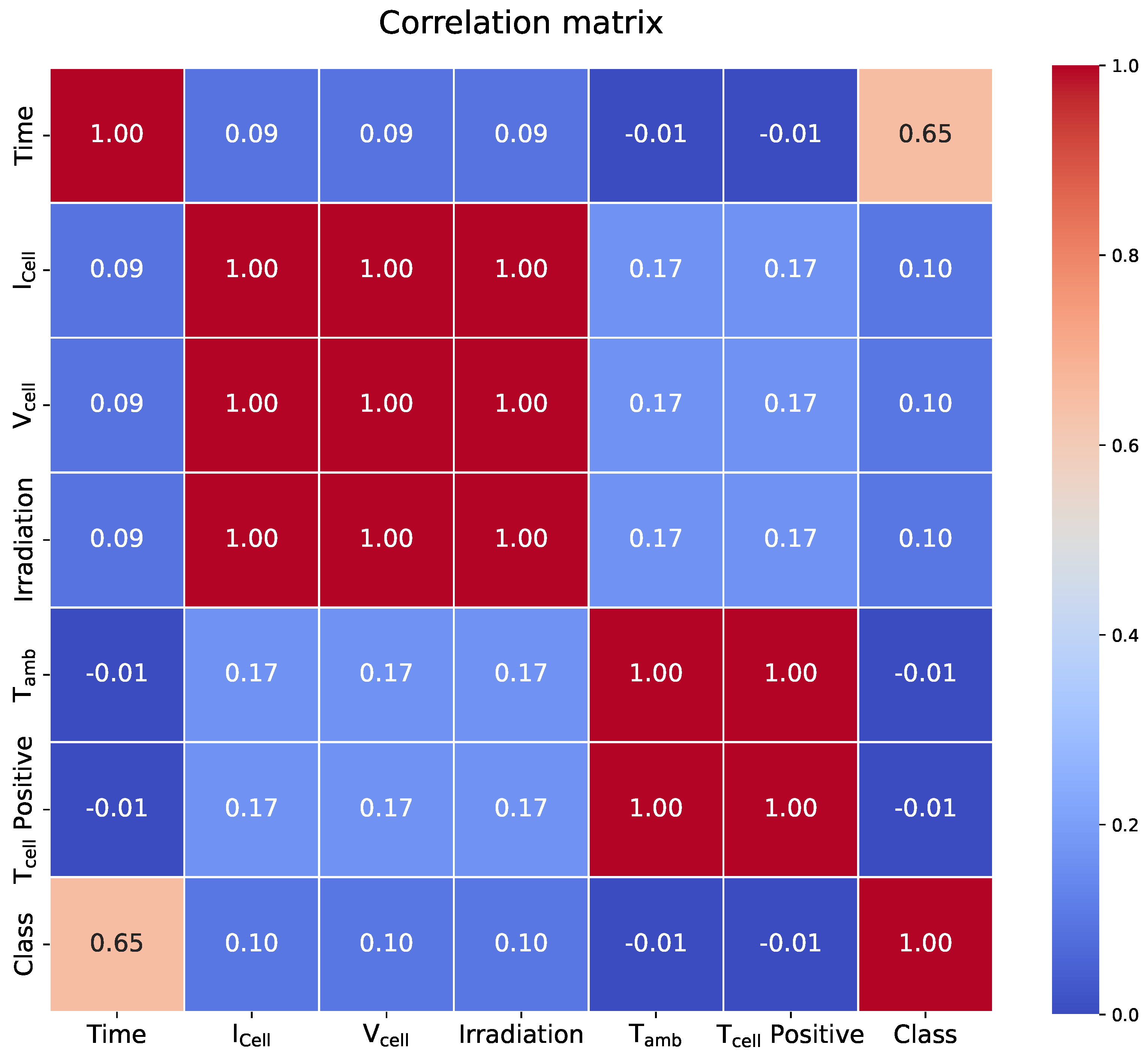
Preprocessing: Features (, , irradiance, , ) are normalized to [0, 1] using MinMaxScaler (scikit-learn version 1.2.2) [26]. ReliefF [14], validated by [27], ranks feature relevance (Table 2), showing and as dominant, with irradiance, , and correlated (Figure 7).
Table 2.
ReliefF scores of each feature.
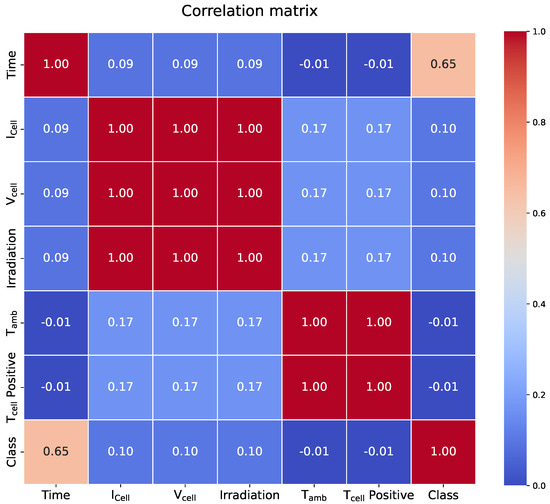
Figure 7.
Correlation matrix of the selected features, highlighting the interdependence between sensor variables such as cell temperature, irradiance, and current.
Model Design: The OFFNN, optimized via Genetic Algorithm (GA) over 50 generations, features two Dense layers (128 and 64 neurons) with ReLU activation, Dropout (0.3) for regularization, and a softmax output for five-class classification. GA optimizes neuron counts and layers, outperforming manual tuning and aligning with neural architecture search trends [28].
Training: The dataset is split (80% training, 20% validation), using categorical cross-entropy loss, Adam optimizer, and EarlyStopping (patience 10 epochs) [29]. Training runs for 100 epochs with internal validation.
3.2. Implementation and Training Details
All experiments were conducted using Python 3.9 with TensorFlow 2.11 and Keras APIs 2.11 (https://keras.io; accessed on 8 June 2025).
Feature selection via ReliefF was implemented using the “skrebate” package [27], while the Genetic Algorithm (GA) optimization followed a custom wrapper built upon “DEAP” and “Optuna” libraries. MinMax scaling and preprocessing were handled with scikit-learn.
The Genetic Algorithm executed 50 generations with a population size of 20, optimizing the number of hidden layers, neuron counts, and dropout rates. This setup achieved better validation performance than manual tuning and aligns with recent developments in Neural Architecture Search (NAS) [28].
Training used categorical cross-entropy loss and the Adam optimizer. Early stopping was applied with a patience of 10 epochs to prevent overfitting [29]. All results reported were validated using a fixed 80/20 training-validation split.
The methodology is designed for reproducibility and scalability. Scripts for data generation, feature ranking, and model training are available upon request to facilitate replication or further study.
Although the synthetic dataset was constructed by independently varying irradiance, temperature, and degradation parameters, we acknowledge that the resulting features may exhibit stronger correlations than observed in real-world scenarios. This is due to the deterministic nature of simulation outputs and the absence of sensor noise or fabrication variances. These factors can lead to idealized patterns that exaggerate feature dependencies.
4. Results and Discussion
4.1. Overall Classification Performance
The OFFNN achieves an overall accuracy of 75.43% on the validation set, as shown in the confusion matrix (Figure 8). Table 3 summarizes precision, recall, and F1-scores for each class. Class 1 (normal operation) exhibits the highest performance, with an F1-score of 0.79, benefiting from real-world data samples. Other classes, representing simulated degradation modes, show good generalization with F1-scores between 0.74 and 0.76.
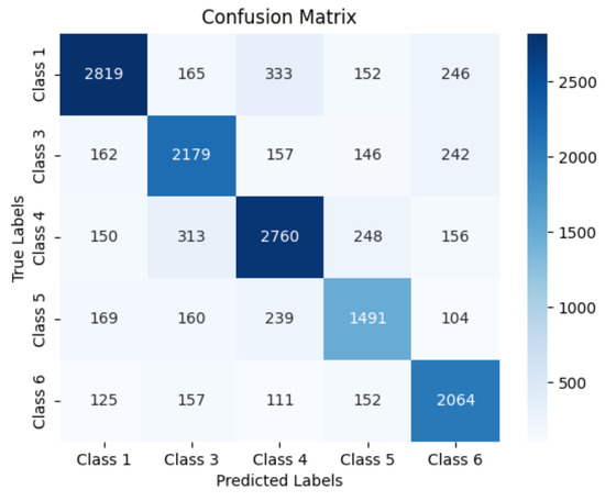
Figure 8.
Confusion matrix showing classification results across the five classes. Numerical labels are retained for consistency with the original model output. Note: The confusion matrix in the figure uses numerical class indices due to consistency with the classification model’s training labels. For improved clarity, the corresponding degradation types are as follows: Class 1—Normal; Class 3—EVA Discoloration; Class 4—Cracks; Class 5—LID; and Class 6—Corrosion. These mappings are also reflected in Table 3, which presents performance metrics using descriptive labels.
Table 3.
Performance metrics (total: 75,000 samples; accuracy: 75.43%).
The results indicate that the hybrid simulation–classification approach is effective in distinguishing between multiple degradation mechanisms using a limited number of physical sensors. The combination of bond graph-based simulation and neural network classification provides a scalable and interpretable method for root-cause identification in PV systems.
It is also important to note that the synthetic dataset, while comprehensive in its coverage of degradation types and environmental variations, may still lack the stochastic complexity of real-world data. For example, Figure 7 shows high correlations (even near-perfect) between certain features like irradiance and cell voltage. Such relationships, while consistent with physical modeling, may not fully reflect sensor variability, measurement noise, or aging effects in actual deployments.
4.2. Class-Wise Performance, Dataset Limitations, and Interpretability
While Class 1, representing Normal, shows high performance due to the availability of real data, the model also performs well in distinguishing other degradation types based on synthetic data. Classes 3 and 4 (e.g., EVA discoloration and cracks) show F1-scores above 0.74, indicating that their impact on the measured signals is distinctive and detectable by the trained network.
Class 5, representing LID, shows the lowest precision (0.68) and F1-score (0.69). This may be attributed to the subtle signal changes induced by LID in early stages, which overlap with other degradations in the feature space. Further improvement could be achieved by enhancing feature extraction techniques or including more detailed thermal-electrical behavior modeling for LID.
These insights confirm that, while some degradation modes are clearly identifiable, others may require advanced preprocessing or more sensitive measurement parameters. Nonetheless, the model demonstrates the ability to generalize from both real and simulated data, highlighting its potential for practical deployment in PV monitoring systems.
While the simulation-based dataset allows for detailed control over fault scenarios and environmental conditions, we acknowledge that the model’s validation is limited by the absence of real-world degraded PV data. This may affect the immediate practical applicability of the classifier, particularly in field conditions where sensor noise, calibration drift, and complex environmental dynamics are present. The current study is intended as a reproducible and modular foundation. Future extensions will aim to incorporate experimental datasets and field measurements to improve robustness and ensure the classifier generalizes effectively to real operational settings.
Another important limitation is the exclusive use of single-fault degradation scenarios in the simulation process. In practice, photovoltaic systems often experience simultaneous or interacting degradation mechanisms, which can result in more complex and ambiguous signal patterns. The current model does not yet address such compound fault scenarios. Furthermore, real sensor measurements are subject to noise, environmental variability, and hardware aging—factors not captured in the clean, synthetic dataset. These issues may reduce the classifier’s robustness and accuracy in field applications. Future work will focus on simulating multi-fault conditions and introducing realistic noise models to better emulate operational environments and improve fault differentiation under non-ideal conditions.
It is also important to distinguish between the interpretability of the physical simulation layer and the neural network classifier. While the bond graph-based degradation modeling enables physically meaningful and transparent feature generation, the OFFNN component, like many deep learning models, functions as a black box. Although feature selection via ReliefF improves understanding of input relevance, the internal decision logic of the network remains opaque. Nevertheless, the use of physically meaningful simulation inputs and feature ranking helps bridge the gap between black-box predictions and physical interpretability, providing partial transparency into the classification process. Future extensions could explore the integration of explainable AI (XAI) techniques such as SHAP values [30] or LIME [31] to provide post-hoc insights into model predictions. Alternatively, inherently interpretable models like decision trees or rule-based classifiers may offer greater transparency [32].
4.3. Comparison with Related Work
Previous studies, such as Mansour et al. [5], have reported classification accuracies of up to 90% using Support Vector Machines (SVMs) applied to curated real-world datasets. While our model exhibits slightly lower overall accuracy, it is trained on a combination of real and synthetic data, making it particularly suitable for scenarios where real faulty samples are scarce or unavailable.
More recent deep learning approaches have explored hybrid architectures—such as convolutional neural networks (CNNs) combined with bidirectional gated recurrent units (Bi-GRU)—which are effective in capturing temporal dependencies in PV system data [33]. Ensemble learning strategies, including deep stacked architectures, have also demonstrated strong generalization performance in complex classification tasks [34].
In contrast, our approach emphasizes a physically informed and modular simulation–classification framework. The use of a Genetic Algorithm for neural architecture optimization, along with ReliefF for feature selection, ensures that the model is well-tuned for both performance and interpretability. This design enables better control over input–output relationships and supports transparent validation across a range of simulated degradation scenarios.
5. Conclusions
This paper presents a hybrid methodology for the detection and identification of degradation root causes in photovoltaic (PV) cells by integrating bond graph-based physical modeling with empirical degradation profiles and deep learning classification. The proposed approach simulates various degradation modes using a modular and scalable framework, generating synthetic datasets to train an optimized feed-forward neural network (OFFNN). The network, enhanced by ReliefF-based feature selection and Genetic Algorithm optimization, successfully classifies degradation types with 75.43% accuracy, demonstrating robustness even in scenarios with limited real-world fault data.
The results confirm the feasibility of combining physical simulations with AI to enable accurate root-cause diagnostics using only standard PV sensor data. The interpretability and modularity of the method make it well-suited for deployment in intelligent PV monitoring and predictive maintenance systems.
Future Work: Future research will focus on extending the simulator to include a broader range of degradation mechanisms, such as potential-induced degradation (PID) under variable humidity and long-term voltage stress, as well as more complex physical phenomena such as delamination. These additions are expected to enhance the realism and practical relevance of the diagnostic framework. Moreover, future extensions may benefit from incorporating multi-modal diagnostic inputs, including infrared thermography, which has shown promise in PV fault detection and classification when combined with deep learning approaches [35]. Additionally, exploring temporal models (e.g., LSTM networks) may enhance the ability to track fault progression over time. Deployment on embedded systems or edge devices for real-time diagnosis is also planned to enable field-level implementation. Finally, future work will investigate noise injection techniques and the use of hybrid datasets that include real-world measurements and sensor noise profiles to improve model robustness and ensure realistic behavior under field conditions.
Author Contributions
Conceptualization, M.D. and N.F.; methodology, M.D. and N.F.; software, N.F.; validation, M.B., H.A.S., and N.M.; formal analysis, M.D.; investigation, M.D. and N.F.; resources, M.B.; data curation, N.F.; writing—original draft preparation, M.D.; writing—review and editing, N.F. and H.A.S.; visualization, N.F.; supervision, M.B. and N.M.; project administration, M.D.; funding acquisition, M.B. All authors have read and agreed to the published version of the manuscript.
Funding
This research received no external funding.
Institutional Review Board Statement
Not applicable.
Informed Consent Statement
Not applicable.
Data Availability Statement
The original contributions presented in this study are included in the article. Further inquiries can be directed to the corresponding author.
Acknowledgments
The authors would like to acknowledge the administrative support provided by Aix-Marseille University, Ankara Medipol University, City University (Tripoli), and the Lebanese University during the course of this research.
Conflicts of Interest
The authors declare no conflicts of interest.
Abbreviations
The following abbreviations are used in this manuscript:
| PV | Photovoltaic |
| LID | Light Induced Degradation |
| EVA | Ethylene-Vinyl Acetate |
| OFFNN | Optimized Feed-Forward Neural Network |
| PCA | Principal Component Analysis |
| SVM | Support Vector Machine |
| PID | Potential Induced Degradation |
| GA | Genetic Algorithm |
Appendix A. Bond Graph Methodology
The bond graph methodology is a graphical formalism for multi-physical system modeling, leveraging causal and structural properties to analyze system behavior and construct simulators [13]. Its key elements include the following:
- Behavior Elements:
- -
- R-element (resistance): Models dissipative effects (e.g., thermal resistance, electrical resistors).
- -
- C-element (capacitance): Represents storage (e.g., thermal mass, capacitance).
- -
- I-element (inertia): Captures inertial effects (rare in PV modeling here).
- Junction Elements:
- -
- 0-junction: Enforces equal effort (e.g., voltage in parallel circuits), summing flows (e.g., currents).
- -
- 1-junction: Enforces equal flow (e.g., current in series), summing efforts (e.g., voltages).
- -
- (transformer), (gyrator): Convert energy between domains.
Causality, assigned by convention, defines cause–effect relationships (e.g., effort-in, flow-out for R-elements). This enables structural analysis and simulation, as applied to the PV cell model in Section 2. For a comprehensive treatment, see [13].
Appendix B. Supporting Material: Detailed Models
This section provides detailed equations for the thermal, electro-thermal, and degradation models referenced in Section 2.
Appendix B.1. Thermal Model Equations
The thermal model uses R-elements for heat distribution along axes (x, y, z):
where is thermal conductivity. The C-element is given by
with as density and c as specific heat.
Appendix B.2. Electro-Thermal Model Equations
Cell current is defined as
where the photocurrent is
with , A as area, as effective irradiance, as standard irradiance, as responsivity, T as cell temperature, and as ambient temperature. The diode current is
with as saturation current, as open-circuit voltage, and , as constants.
Appendix B.3. Degradation Models
- Ageing [9]:
- Shunt resistance:
- Series resistance:
- EVA Discoloration [10]:
- LID [6]:
- Cracking [12,21,22]:
- , ,
- Corrosion [11]:
- , ,
- Potential Induced Degradation (PID) [7]:
- where is the initial shunt resistance, is the system voltage, t is time, and is a degradation rate constant.
References
- Li, B.; Delpha, C.; Migan-Dubois, A.; Diallo, D. Fault diagnosis of photovoltaic panels using full I–V characteristics and machine learning techniques. Energy Convers. Manag. 2021, 248, 114785. [Google Scholar]
- Lu, X.; Lina, P.; Cheng, S.; Fang, G.; He, X.; Chen, Z.; Wu, L. Fault diagnosis model for photovoltaic array using a dual-channels convolutional neural network with a feature selection structure. Energy Convers. Manag. 2021, 248, 114777. [Google Scholar]
- Hong, Y.-Y.; Pula, R.A. Methods of photovoltaic fault detection and classification: A review. Energy Rep. 2022, 8, 5898–5929. [Google Scholar]
- Li, B.; Delpha, C.; Diallo, D.; Migan-Dubois, A. Application of Artificial Neural Networks to photovoltaic fault detection and diagnosis: A review. Renew. Sustain. Energy Rev. 2021, 138, 110512. [Google Scholar]
- Hajji, M.; Harkat, M.-F.; Kouadri, A.; Abodayeh, K.; Mansouri, M.; Nounou, H.; Nounou, M. Multivariate feature extraction based supervised machine learning for fault detection and diagnosis in photovoltaic systems. Eur. J. Control 2021, 59, 313–321. [Google Scholar]
- Sopori, B.; Basnyat, P.; Devayajanam, S.; Shet, S.; Mehta, V.; Binns, J.; Appel, J. Understanding light-induced degradation of c-Si solar cells. In Proceedings of the 38th IEEE Photovoltaic Specialists Conference, Austin, TX, USA, 3–8 June 2012; pp. 587–615. [Google Scholar]
- Damiani, B.; Nakayashiki, K.; Kim, D.S.; Yelundur, V.; Ostapenko, S.; Tarasov, I.; Rohatgi, A. Light induced degradation in promising multi-crystalline silicon materials for solar cell fabrication. In Proceedings of the 3rd World Conference on Photovoltaic Energy Conversion, Osaka, Japan, 11–18 May 2003; pp. 1483–1510. [Google Scholar]
- Fuentes-Morales, R.F.; Diaz-Ponce, A.; Cruz, M.I.P.; Rodrigo, P.M.; Valentin-Coronado, L.M.; Martell-Chavez, F.; Pineda-Arellano, C.A. Control algorithms applied to active solar tracking systems: A review. Sol. Energy 2020, 212, 203–219. [Google Scholar]
- Logerais, P.-O.; Riou, O.; Doumane, R.; Balistrou, M.; Durastanti, J.-F. Étude par simulation de l’influence du vieillissement et des conditions climatiques sur la production électrique d’un module photovoltaïque. In Proceedings of the JiTH 2013, Marrakesh, Morocco, 13–15 November 2013. [Google Scholar]
- Pern, F.J. Factors that affect the EVA encapsulant discoloration rate upon accelerated exposure. Sol. Energy Mater. Sol. Cells 1996, 41–42, 587–615. [Google Scholar]
- Braisaz, B.; Duchayne, C.; Van Iseghem, M.; Khalid, R. PV aging model applied to several meteorological conditions. In Proceedings of the 29th European Photovoltaic Solar Energy Conference and Exhibition (EU PVSEC 2014), Amsterdam, The Netherlands, 22–26 September 2014. [Google Scholar]
- Papargyri, L.; Papanastasiou, P.; Georghiou, G.E. Effect of materials and design on PV cracking under mechanical loading. Renew. Energy 2022, 199, 433–444. [Google Scholar]
- Karnopp, D.; Margolis, D.; Rosenberg, R. System Dynamics: Modeling, Simulation, and Control of Mechatronic Systems, 5th ed.; John Wiley and Sons: Hoboken, NJ, USA, 2012. [Google Scholar]
- Kononenko, I. Estimating attributes: Analysis and extensions of RELIEF. In Lecture Notes in Computer Science; Springer: Berlin/Heidelberg, Germany, 1994; pp. 171–182. [Google Scholar]
- Schmidhuber, J. Deep learning in neural networks: An overview. Neural Netw. 2015, 61, 85–117. [Google Scholar]
- Ciulla, G.; Brano, V.L.; Di Dio, V.; Cipriani, G. A comparison of different one-diode models for the representation of I–V characteristic of a PV cell. Renew. Sustain. Energy Rev. 2014, 32, 684–696. [Google Scholar]
- Tina, G.M.; Scandura, P.F. Case study of a grid connected with a battery photovoltaic system: V-trough concentration vs. single-axis tracking. Energy Convers. Manag. 2012, 64, 569–578. [Google Scholar]
- Rosa-Clot, M.; Rosa-Clot, P.; Tina, G.M.; Scandura, P.F. Submerged photovoltaic solar panel: SP2. Renew. Energy 2010, 35, 1862–1865. [Google Scholar]
- Tina, G.M.; Scavo, F.B.; Merlo, L.; Bizzarri, F. Comparative analysis of monofacial and bifacial photovoltaic modules for floating power plants. Appl. Energy 2021, 281, 116084. [Google Scholar]
- Le, P.-T.; Tsai, H.-L.; Le, P.-L. Development and Performance Evaluation of Photovoltaic (PV) Evaluation and Fault Detection System Using Hardware-in-the-Loop Simulation for PV Applications. Micromachines 2023, 14, 674. [Google Scholar] [CrossRef]
- Paggi, M.; Corrado, M.; Rodriguez, M.A. A multi-physics and multi-scale numerical approach to microcracking and power-loss in photovoltaic modules. Compos. Struct. 2013, 95, 630–638. [Google Scholar]
- Katayama, N.; Osawa, S.; Matsumoto, S.; Nakano, T.; Sugiyama, M. Degradation and fault diagnosis of photovoltaic cells using impedance spectroscopy. Sol. Energy Mater. Sol. Cells 2019, 194, 130–136. [Google Scholar]
- Al Mahdi, H.; Leahy, P.G.; Alghoul, M.; Morrison, A.P. A Review of Photovoltaic Module Failure and Degradation Mechanisms: Causes and Detection Techniques. Solar 2024, 4, 43–82. [Google Scholar] [CrossRef]
- Buda, M.; Maki, A.; Mazurowski, M.A. A systematic study of the class imbalance problem in convolutional neural networks. Neural Netw. 2018, 106, 249–259. [Google Scholar]
- Djeziri, M.A.; Djedidi, O.; Morati, N.; Seguin, J.L.; Bendahan, M.; Contaret, T. A temporal-based SVM approach for the detection and identification of pollutant gases in a gas mixture. Appl. Intell. 2022, 52, 6065–6078. [Google Scholar] [CrossRef]
- Ioffe, S.; Szegedy, C. Batch Normalization: Accelerating Deep Network Training by Reducing Internal Covariate Shift. In Proceedings of the 32nd International Conference on Machine Learning (ICML’15), Lille, France, 6–11 July 2015; pp. 448–456. [Google Scholar]
- Urbanowicz, R.J.; Olson, R.S.; Schmitt, P.; Meeker, M.; Moore, J.H. Benchmarking relief-based feature selection methods for bioinformatics data mining. J. Biomed. Inform. 2018, 85, 168–188. [Google Scholar] [CrossRef]
- Real, E.; Moore, S.; Selle, A.; Saxena, S.; Suematsu, Y.L.; Tan, J.; Le, Q.V.; Kurakin, A. Regularized Evolution for Image Classifier Architecture Search. Proc. Aaai Conf. Artif. Intell. 2019, 33, 4780–4789. [Google Scholar]
- Prechelt, L. Early Stopping—But When? In Neural Networks: Tricks of the Trade, 2nd ed.; Montavon, G., Orr, G.B., Müller, K.-R., Eds.; Springer: Berlin/Heidelberg, Germany, 2012; pp. 53–67. [Google Scholar]
- Lundberg, S.M.; Lee, S.-I. A unified approach to interpreting model predictions. In Proceedings of the 31st International Conference on Neural Information Processing Systems (NeurIPS), Long Beach, CA, USA, 4–9 December 2017; pp. 4765–4774. [Google Scholar]
- Ribeiro, M.T.; Singh, S.; Guestrin, C. “Why should I trust you?”: Explaining the predictions of any classifier. In Proceedings of the 22nd ACM SIGKDD International Conference on Knowledge Discovery and Data Mining, San Francisco, CA, USA, 13–17 August 2016; pp. 1135–1144. [Google Scholar]
- Guidotti, R.; Monreale, A.; Ruggieri, S.; Turini, F.; Giannotti, F.; Pedreschi, D. A survey of methods for explaining black box models. ACM Comput. Surv. (Csur) 2018, 51, 93. [Google Scholar]
- Amiri, A.F.; Kichou, S.; Oudira, H.; Chouder, A.; Silvestre, S. Fault Detection and Diagnosis of a Photovoltaic System Based on Deep Learning Using the Combination of a Convolutional Neural Network (CNN) and Bidirectional Gated Recurrent Unit (Bi-GRU). Sustainability 2024, 16, 1012. [Google Scholar] [CrossRef]
- Lodhi, E.; Wang, F.-Y.; Xiong, G.; Zhu, L.; Tamir, T.S.; Rehman, W.U.; Khan, M.A. A Novel Deep Stack-Based Ensemble Learning Approach for Fault Detection and Classification in Photovoltaic Arrays. Remote Sens. 2023, 15, 1277. [Google Scholar] [CrossRef]
- Boubaker, S.; Kamel, S.; Ghazouani, N.; Mellit, A. Assessment of Machine and Deep Learning Approaches for Fault Diagnosis in Photovoltaic Systems Using Infrared Thermography. Remote Sens. 2023, 15, 1686. [Google Scholar] [CrossRef]


Disclaimer/Publisher’s Note: The statements, opinions and data contained in all publications are solely those of the individual author(s) and contributor(s) and not of MDPI and/or the editor(s). MDPI and/or the editor(s) disclaim responsibility for any injury to people or property resulting from any ideas, methods, instructions or products referred to in the content. |
© 2025 by the authors. Licensee MDPI, Basel, Switzerland. This article is an open access article distributed under the terms and conditions of the Creative Commons Attribution (CC BY) license (https://creativecommons.org/licenses/by/4.0/).