Numerical Weather Modelling and Large Eddy Simulations of Strong-Wind Events in Coastal Mountainous Terrain

Featured Application

High-resolution weather models and large eddy simulations are critical for accurate modelling of wind and wind power production in complex terrain. Standard mesoscale numerical weather modelling tends to underestimate high-wind events, while increased resolution in the model allows for a more accurate terrain representation and capture of localised wind effects in the area.

Abstract

This study investigates high-resolution numerical weather modelling and large eddy simulations (LESs) for wind resource assessment in complex coastal mountainous terrain. The main purpose is to investigate strong-wind events, where earlier research indicates that high wind speeds are underestimated. Using the Weather Research and Forecasting model (WRF), simulations were conducted for the Fakken wind power plant in northern Norway, a region characterised by steep mountains, fjords, and challenging wind patterns. The study evaluates the impact of increasing model resolution, from mesoscale to LESs, on wind speed and power production estimates. Results show that higher-resolution models improve the representation of terrain features, leading to better estimations of wind speed and direction, particularly during strong-wind events such as the Ylva storm in 2017. The LES model demonstrated the ability to capture high-wind events, including localised speed-ups and lee-side amplification, which is critical for accurate wind speed modelling. Comparison with power production data shows the potential of WRF LESs to optimise wind farm operations in complex terrains.

1. Introduction

Wind power is the second largest renewable energy resource, with a market share of 7.8%, or about 2325 TWh, of the total electricity production in the world in 2023 [1], and a global increase in installed wind power capacity of 11%, from 1021 GW to 1136 GW, in 2024 [2]. As an intermittent resource, wind power production strongly depends on the local wind conditions, and wind resource assessment is an important part of the development of new wind farms. There are several options for wind resource assessment, including observational data from wind measurements, numerical weather modelling (NWM) and/or computational fluid dynamics, followed by statistical post-processing of one or a combination of these methods [3,4,5]. A common setup for wind resource assessment for a wind power plant is to use locally measured data, and then microscale numerical wind simulations to determine wind variations in the area for optimal placement of wind turbines [6,7,8,9].

During the last decade, numerical weather models have proven to be a natural step for mesoscale wind resource assessment when considering large areas and/or long time intervals [10], as in country-wide wind atlases for Spain [11], Finland [12], Greece [13], Canada [14,15] and Russia [16]. Several reports show that the differences between NWM and site-specific wind measurements are in the order of 5% or less [10], although complex terrain typically increases the errors [8,11,17,18]. Already in this early period of NWM for mapping, ref. [11] performed validation test of a wind map based on the mesoscale Skiron against measurement masts in different terrain types in Spain. This showed that the mean average error was larger, and with more spread, for complex terrain compared to flat terrain. Ref. [8] used two wind power park locations in complex terrain, with measurements from several wind turbines and meteorological masts for comparison, and showed that the Weather Research and Forecasting model (WRF) resulted in improved wind speed estimates compared to the commercial microscale models WindSim and WAsP.

One of the great advantages of NWM is that it typically includes global coverage where meteorological measurements are incorporated, and although these measurements might be far from the site under scrutiny, the physical modelling allows for downscaling and creation of virtual mast data that can successfully be used individually for weather research assessment [8] or as input for traditional microscale computational fluid dynamics (CDF) modelling for wind power [12,18]. With increasing computational power, NWM has moved into the microscale flow regime where parametric planetary boundary layer parametrisation is replaced by large eddy simulations (LESs) to resolve terrain effects [19,20] and/or includes wind turbines in the wind field [21,22,23,24]. The case study in [20] shows how WRF LESs can be used to study the wind changes over 42 h for 274 individual wind turbine locations at one wind park in a mountainous area. Thus, NWM may be able to provide an initial detailed wind resource assessment without the need for site measurements or additional microscale software tools such as WAsP for the New European Wind Atlas [25]. Although several papers have studied and used NWM for wind power applications, its tendency to underestimate high-wind-speed events has recently been reported in both complex terrain [26,27] and offshore [28,29].

In this paper, we investigate the mesoscale Weather Research and Forecasting model (WRF) [30] using the Fakken wind power plant located in complex terrain in northern Norway. This site is surrounded by several fjords and steep mountains, and the effect of increased resolution and LESs on the modelled wind flow is compared with measurements during the year of 2017. The final high-resolution WRF-LES model is then evaluated with respect to strong wind measurements from this area, and energy production from turbines of the wind power plant is compared to modelled production using power curves from the turbines at Fakken wind power plant.

2. Materials and Methods

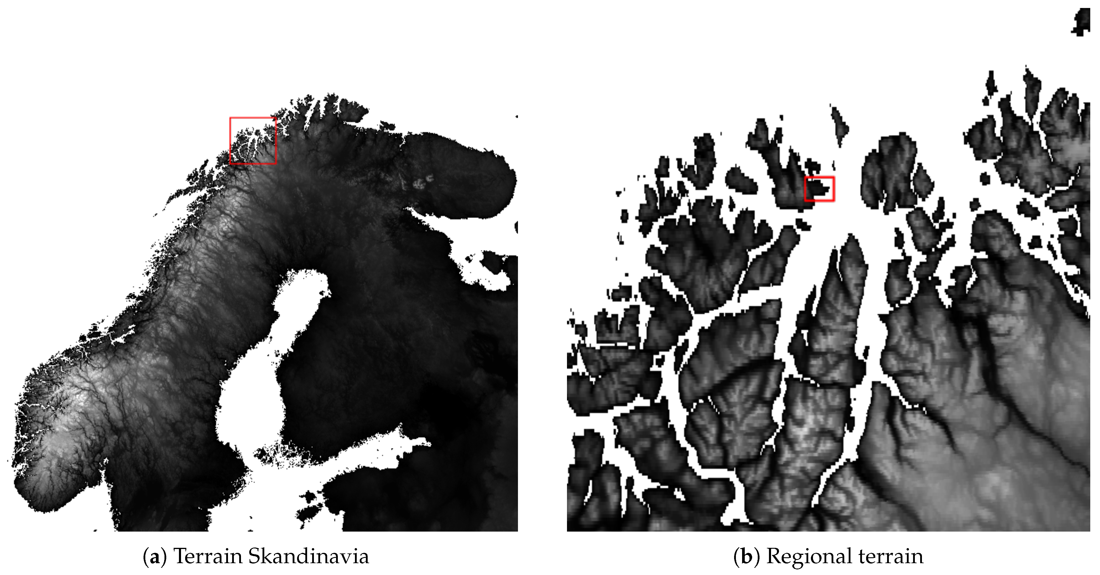
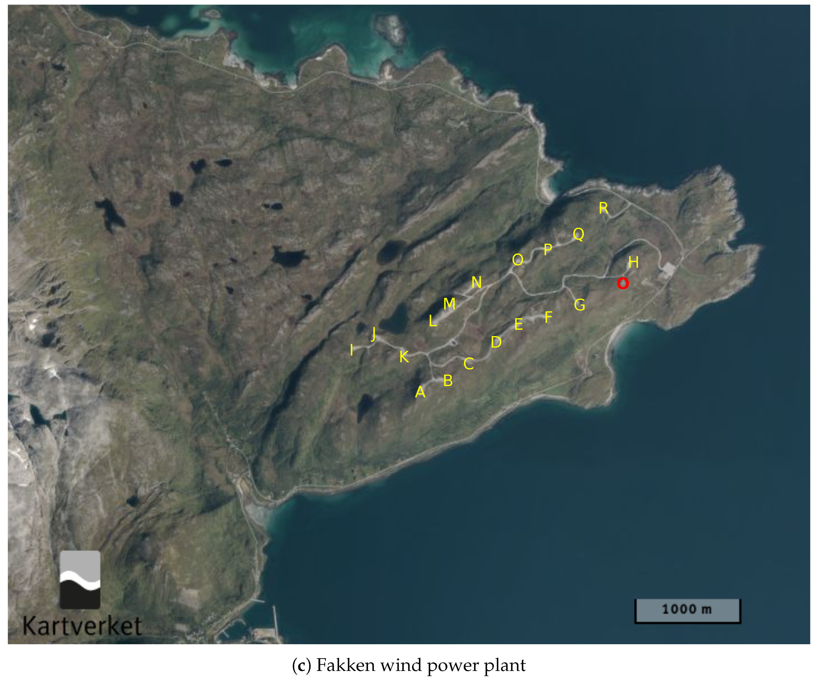
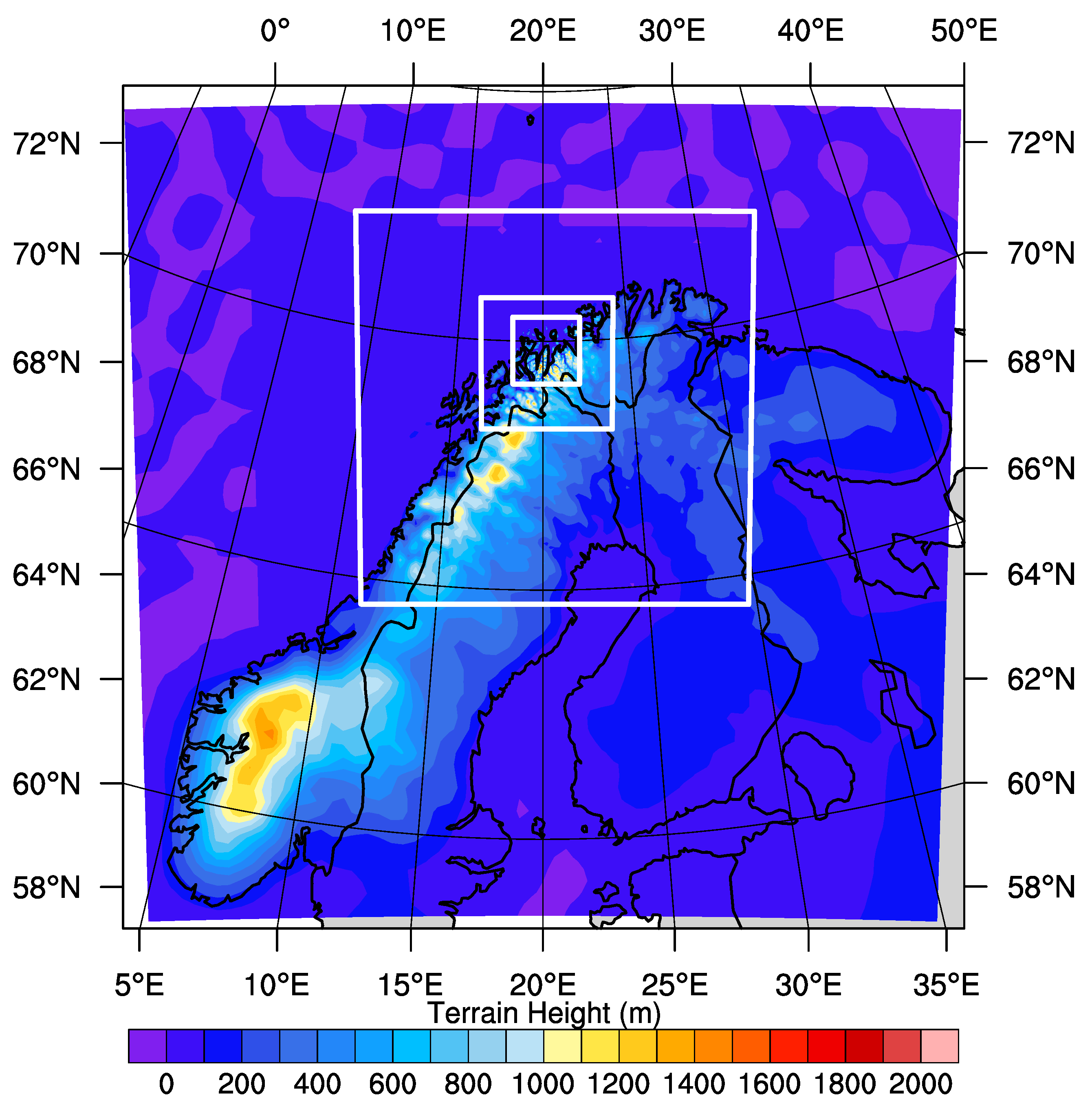
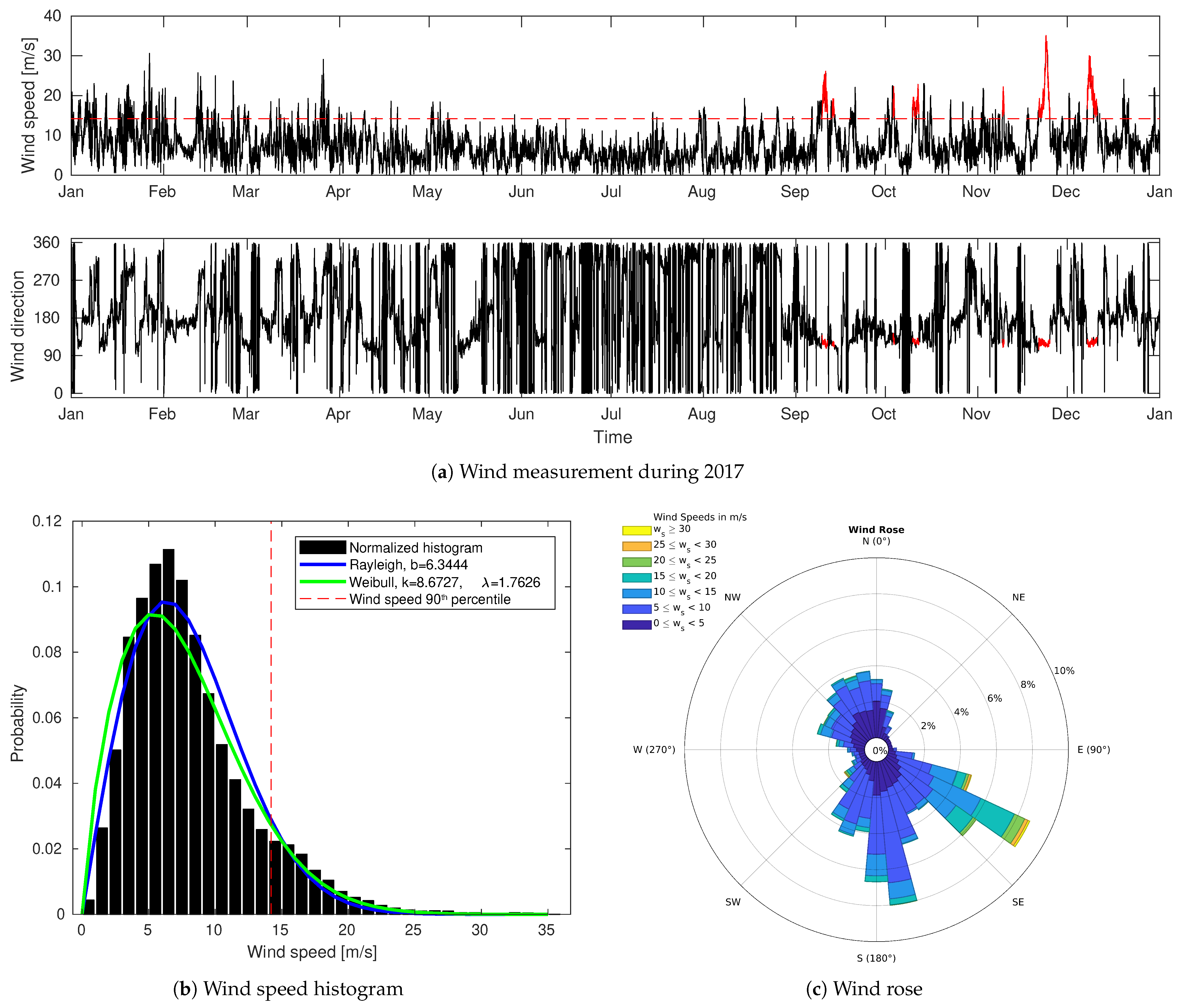
2.1. Site Description

The Scandinavian Peninsula, comprising Norway and Sweden, is shown in Figure 1a together with parts of Finland and Russia. The white colour shows sea level and the brightness from black to white shows terrain heights from sea level up to 2500 m. The peninsula is bordered by the Barents Sea, the Norwegian Sea, the North Sea and Baltic Sea to the north, west, south and east, respectively. Norway has a long coastline with several fjords and valleys that extend into the Scandinavian Mountains, a rugged landscape that is significantly different from Sweden where the terrain in general drops smoothly from this mountain range into the Baltic Sea.

The regional terrain in Figure 1b shows the coastal terrain in northern Norway corresponding to the red rectangle in Figure 1a, and Fakken wind power plant is located at approximately 70° north latitude and 20° east longitude marked with a red rectangle in this regional terrain plot. There are several fjords and mountains that influence the wind at this point. Vannkista is 5 km west and has an elevation of 947 masl and Trolldalstinden is 12 km east (898 masl), both surrounded by similar mountains creating natural barriers to surface-level zonal wind. Starting about 20 km south-southeast, the Lyngen Alps are a dominant mountain range that has several mountains with elevations of 1500–1800 m, which drop abruptly into the 82 km long Lyngen Fjord to the east and 75 km long Ullsfjord to the west. These fjords are prone to meridional surface wind, and the mountain range can create lee spots in the fjords in cases of zonal wind in the atmosphere.

An aerial photo of the Fakken wind power plant is shown in Figure 1c. The measured wind speeds are taken at 80 magl from a meteorological mast located at 70.099° N and 20.093° E at 60 masl, which corresponds to the red circle in Figure 1c. The park consists of 18 Vesta V90 3 MW wind turbines with a nacelle height of 80 magl, which are roughly located along two lines along a small hill with elevation increasing from 20 m to about 200 m starting just north of the mast and in a west-southwest direction. Note that the south line of wind turbines has a quite steep slope down to the sea level, and that the local terrain within the park has several small hills and depressions.

In situ measurements of wind speed and direction are gathered using a Vaisala Anemometer WAA151 and Wind Vane WAV151, respectively. The mean, variance, minimum and maximum values are calculated every 10 min, and time-stamped at the start of the 10 min measurement period. A full year of data from 2017 is used to capture the yearly variation. Fakken wind power plant is in a sub-Arctic climate, where winter temperatures are moderated and mild for the latitude due to the warming effect of the Gulf stream, and the measurements and wind turbines are generally not affected by icing events. The average daily low and high temperatures vary from −6 to 16 °C over the year. Due to the high latitude of this site, the wind is less affected by diurnal patterns. The site also has two months of midnight sun in the summer and two months of winter polar nights, where the sun does not dip below or rise above the horizon, respectively.

2.2. Power Curves and High-Wind Events

The available power in the wind comes from the kinetic energy in the air mass passing through a wind turbine and can be written as

$$P\left(w\right)={\displaystyle \frac{\pi }{2}}\rho r^2{w}^3,$$

(1)

where $\rho$ [kg/m³] is the air density, r [m] is the radius of the wind turbine blades, and w [m/s] is the wind speed. The theoretical maximum power that can be taken out of by the wind turbine is given by Betz’s limit, but in general, a wind turbine-specific power curve $PC\left(w\right)$ is used to describe the power output as blade shape, control systems, generator size and other design options that place additional limits on the power production for a given turbine. The power curve can be modelled based on the turbine hub height wind speed [31], and a simplified description of its shape following [32] is

$$PC\left(w\right)=\left\{\begin{array}{cc}0,\hfill & \mathrm{if}w\le w_{in}\mathrm{or}w\ge w_{out}\hfill \\ P\left(w\right)C_P\left(w\right),\hfill & \mathrm{if}w\in 〈w_{in},w_R〉\hfill \\ P_R,\hfill & \mathrm{if}w\in \left[w_R,w_{out}\right.〉\hfill \end{array}\right.$$

(2)

where the wind speeds $w_{in}$ and $w_{out}$ are the lowest and highest speeds at which the turbine produces power, i.e., the cut-in and cut-out wind speeds, respectively; $P_R$ and $w_R$ are the rated power and rated wind speed of the turbine, respectively; and $C_P\left(w\right)$ is the power coefficient of the turbine. Note that $C_P$ is limited in value to $\left[0,19/27\right.〉$, and that $PC\left(w\right)$ in general can be said to follow an S- or sigmoid-shaped curve up to $w_R$.

Wind speeds around the rated wind are important to identify as these may result in large and rapid changes in power production. In this paper, we will focus on high-wind events defined as the 10 longest continuous events with wind speed measurements above the 90th percentile wind speed.

2.3. Mesoscale Numerical Weather Modelling

The Weather Research and Forecasting (WRF) mesoscale model was developed by the National Center for Atmospheric Research (NCAR) with users and contributions from several meteorological institutions around the world. The version used in this work is v3.9.1, and the simulations are set up as a one-way nested run with 4 domains, D01–D04, as shown in Figure 2. The horizontal resolutions are 27, 9, 3 and 1 km, respectively, all domains with 70 vertical levels, using the Global Multi-resolution Terrain Elevation Data (GMTED) at a 30-arcsecond resolution.

The planetary boundary layer (PBL) is modelled using Mellor Yamada Nakanishi and Niino (option 5) to provide sub-grid TKE terms [33]. The following options were used for the additional physics options: microphysics using the Thompson scheme (option 8) [34], long- and shortwave radiation using the fast Rapid Radiative Transfer Model (option 24) [35], Noah Land Surface Model (option 2) [36], surface layer using the revised MM4 scheme (option 1) [37], and cumulus parameterisation using Kain–Fritsch scheme (option 1) [38].

The ERA interim reanalysis data with 6 h temporal sampling from the European Centre for Medium-Range Weather Forecasts (ECMWF) was used as initial and boundary inputs to the WRF model, and daily simulations were set up with a 12 h spin-up time. Model results were saved every 10th minute, and a full year of time series was created using the daily simulations with a linear interpolation for the last 6 h of the spin-up time for all relevant parameters. Vertical linear interpolation was used to get from the WRF model pressure-based eta level to the 80 magl height, and horizontal bilinear interpolation was used to obtain the latitudes and longitudes of the location of the measurement mast and wind turbines.

Large Eddy Simulations

A higher spatial resolution in a numerical weather model can follow the terrain variations and capture large eddies in the atmospheric flow. In WRF, large eddy simulations (LESs) are applied by turning off the planetary boundary layer scheme, and the terrain height of the inner D05 domain enclosing the Fakken wind power plant is shown as a black rectangular box in Figure 3. The LES model domain is set up with a 3d Smagorinsky diagnostic K for sub-grid turbulence (km_opt = 3), the recommended diffusion option for complex terrain (diff_opt = 2), and sound-wave damping to allow for steep hills (epssm = 0.8).

The horizontal resolution in D05 is 90.9 m, a nesting factor of 11 from the D04 1 km resolution, avoiding the “terra incognita” with spatial resolution in the range of 0.1–1 km where neither PBL parameterisation nor LES is optimal for modelling turbulence [39,40]. The LES domain has $254\times 154$ cells, covering approximately $23\times 14$ km. The 30-arcsecond resolution in GMTED corresponds to approximately 900 m along the latitude lines, which is suitable for the D03–D04 WRF domains. For the D05 domain, the Norwegian Digital Terrain Model (NDTM) with a 10 m resolution is used as input. The 70 vertical levels used in the WRF domains are the pressure-based eta levels, where vertical stretching results in the lowest layers with a thickness below the 90.9 m horizontal resolution.

LESs are generally computationally intensive, and special care must be taken to avoid numerical instabilities from the steep mountains in complex terrain. In this research, we have restricted the LESs to cover the ten longest high-wind-speed events found in the wind measurements during 2017. This allows us to study high-wind-speed measurements whilst at the same time ensuring that the measurements belong to a continuous event. Such events are easier to simulate and analyse than spread-out strong-wind measurements over a longer duration.

2.4. Evaluation of Model Results

Let w be the horizontal wind described as a complex quantity $w=u+iv$, where u and v are the zonal and meridional wind speeds, respectively, and i is the complex identity $i=\sqrt{-1}$. The wind speed $w_s$ and meteorological wind direction $w_d$ can now be defined as

$$\begin{array}{cc}\hfill w_s=\left|w\right|& =\sqrt{u^2+v^2}\hfill \end{array}$$

(3)

$$\begin{array}{cc}\hfill w_d=\angle w& =\mathtt{atan}\mathtt{2}\left(u,v\right){\displaystyle \frac{180}{\pi }}+180,\hfill \end{array}$$

(4)

where $\mathtt{atan}\mathtt{2}$ is the 2-argument arctangent function that provides an output in the range $\left\{-\pi ,\pi \right]$. Note that we transform to degrees and add 180 degrees so that $w_d$ describes the meteorological wind direction, i.e., the direction the wind comes from.

Let $x\left[n\right]$ represent a time series consisting of $n=1,2,\dots ,N$ data points. The sample mean $\overline{x}$ and standard deviation (STD) of $x\left[n\right]$ are

$$\begin{array}{cc}\hfill \overline{x}& ={\displaystyle \frac{1}{N}}\sum _{n=1}^{N}x\left[n\right]\hfill \end{array}$$

(5)

$$\begin{array}{cc}\hfill STD& =\sqrt{{\displaystyle \frac{1}{N}}{\displaystyle \sum _{n=1}^N}{\left(x\left[n\right]-\overline{x}\right)}^2}\hfill \end{array}$$

(6)

Similarly, the root mean square error (RMSE) and correlation coefficient R between the original time series $x\left[n\right]$ and a model $y\left[n\right]$ can be found as

$$\begin{array}{cc}\hfill RMSE& =\sqrt{{\displaystyle \frac{1}{N}}{\displaystyle \sum _{n=1}^N}{\left(x\left[n\right]-y\left[n\right]\right)}^2}\hfill \end{array}$$

(7)

$$\begin{array}{cc}\hfill R& ={\displaystyle \frac{{\sum }_{n=1}^N(x\left[n\right]-\overline{x})(y\left[n\right]-\overline{y})}{\sqrt{{\sum }_{n=1}^N{(x\left[n\right]-\overline{x})}^2{\sum }_{n=1}^N{(y\left[n\right]-\overline{y})}^2}}}.\hfill \end{array}$$

(8)

3. Results and Discussion

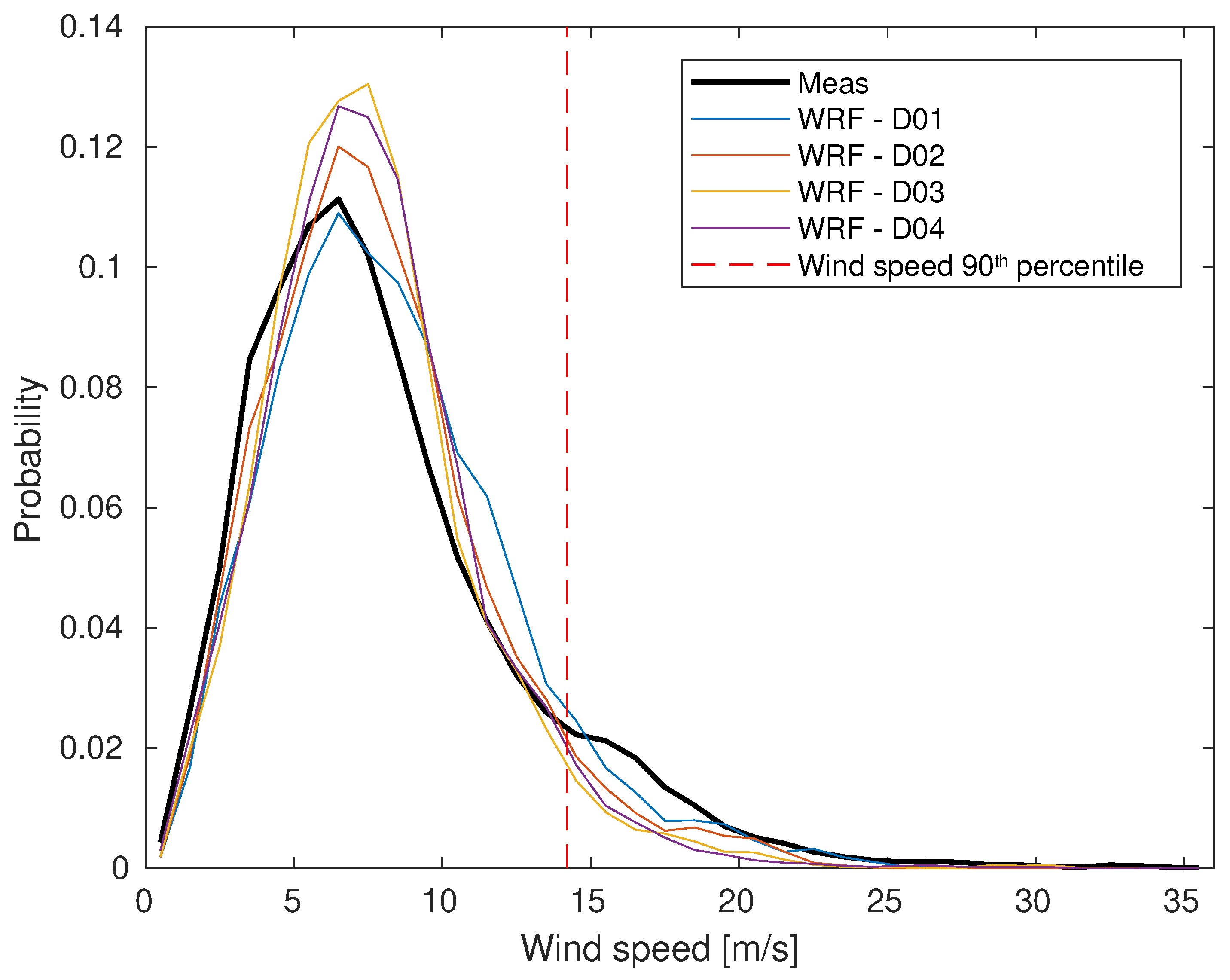
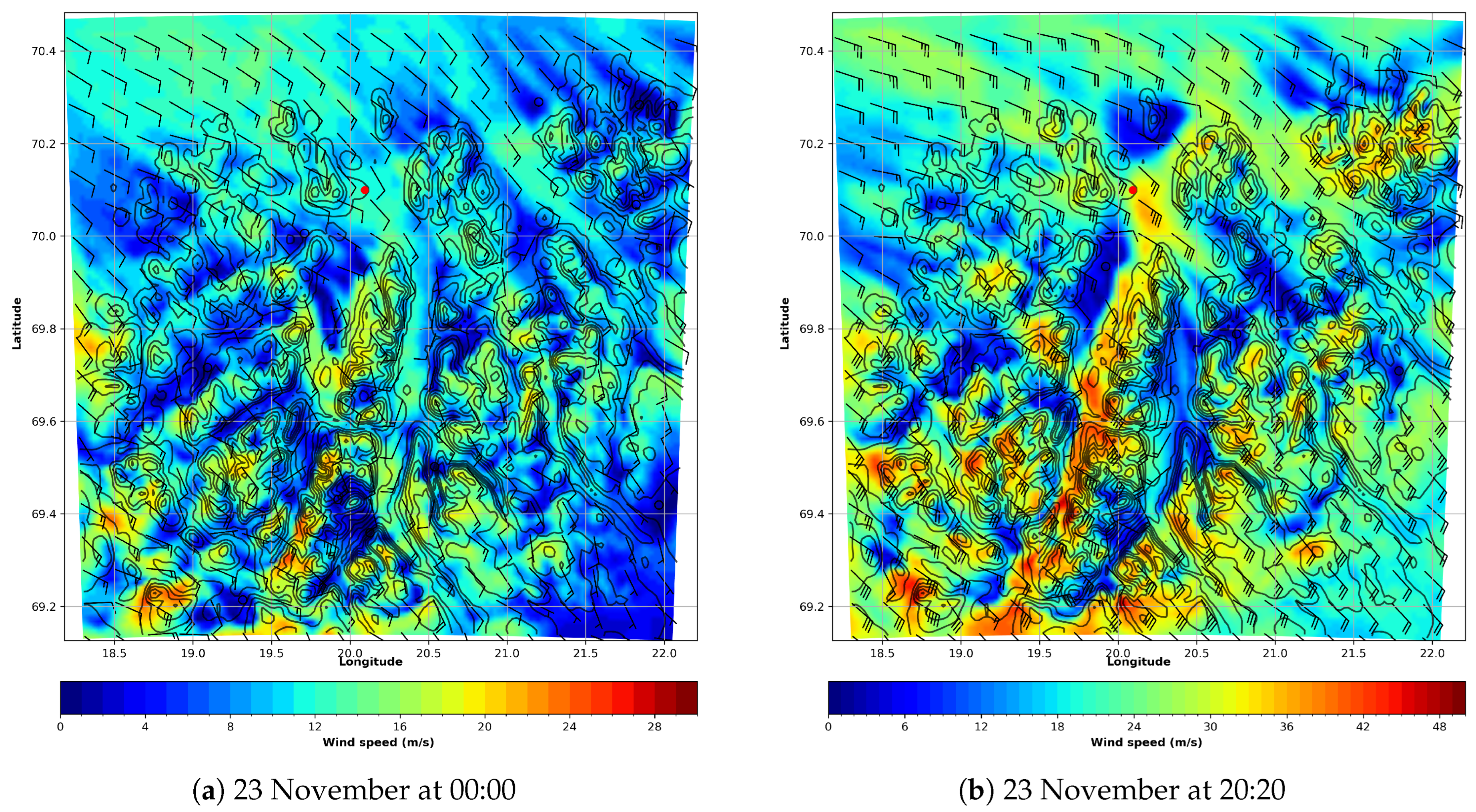
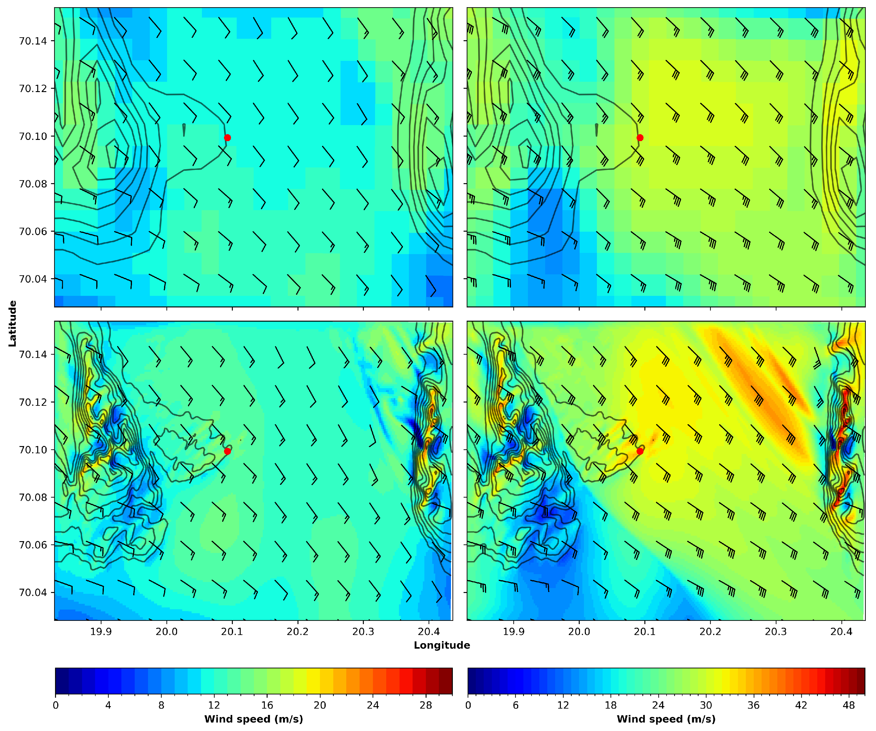
3.1. Model Horizontal Resolution

The terrain height from the NDTM inside the LES domain is shown in plot a) of Figure 4, where the red circle marks the location of the meteorological mast. Although a large part of the domain consists of ocean, the terrain also includes mountains to the west and east of the meteorological mast which have steep inclines as seen by the dense contour lines at 100-metre height differences.

Plots (b), (c) and (d) in Figure 4 show the model terrain height for the same location from D03, D04 and D05, respectively. The 3 × 3 km resolution in plot (b) is clearly visible in the D03 terrain model, and the large grid smooths the terrain so that the mountains are lowered to 450 masl from the original 950 masl. Increasing the resolution to 1 × 1 km in the model, shown in plot (c), increases the height and steepness of the mountains, but they still have a rounded shape. The LES is run with the terrain shown in plot (d), where the mountain shape is more distinct with a steeper increase going up to 900 masl. Note that the GMTED 30-arcsecond resolution corresponds to approximately 900 m horizontal resolution, and that it is important to ensure that the terrain input resolution is equal to or better than the model resolutions. A LES model with GMTED input will result in terrain heights close to the plot in (c), and similarly for a mesoscale model with a 1 km resolution based on NDTM input.

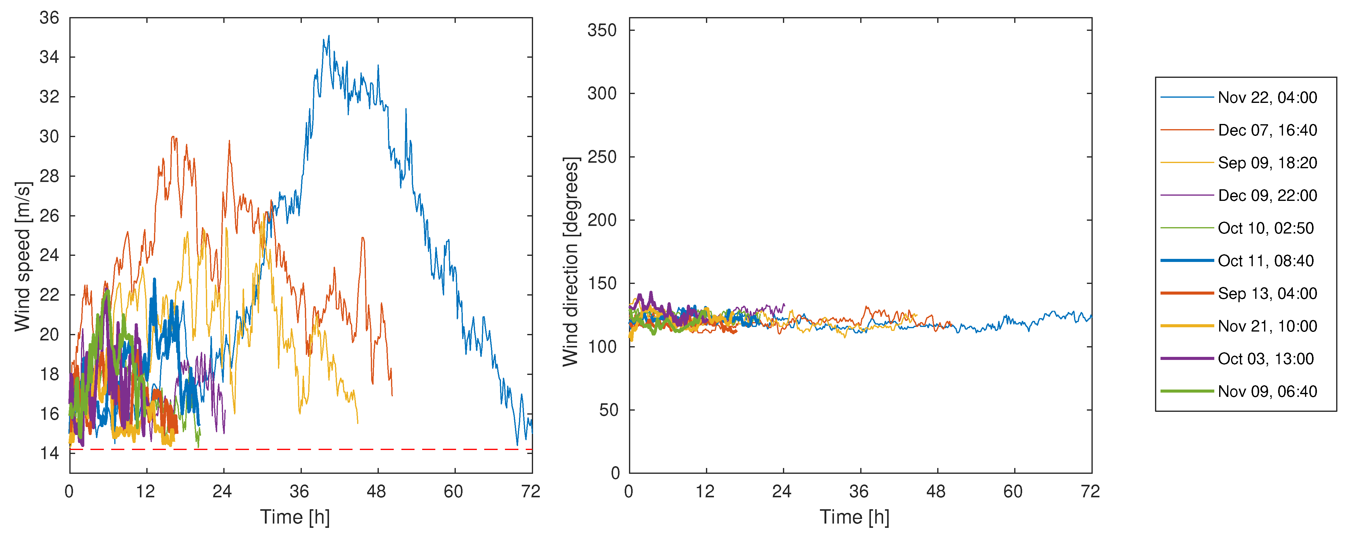
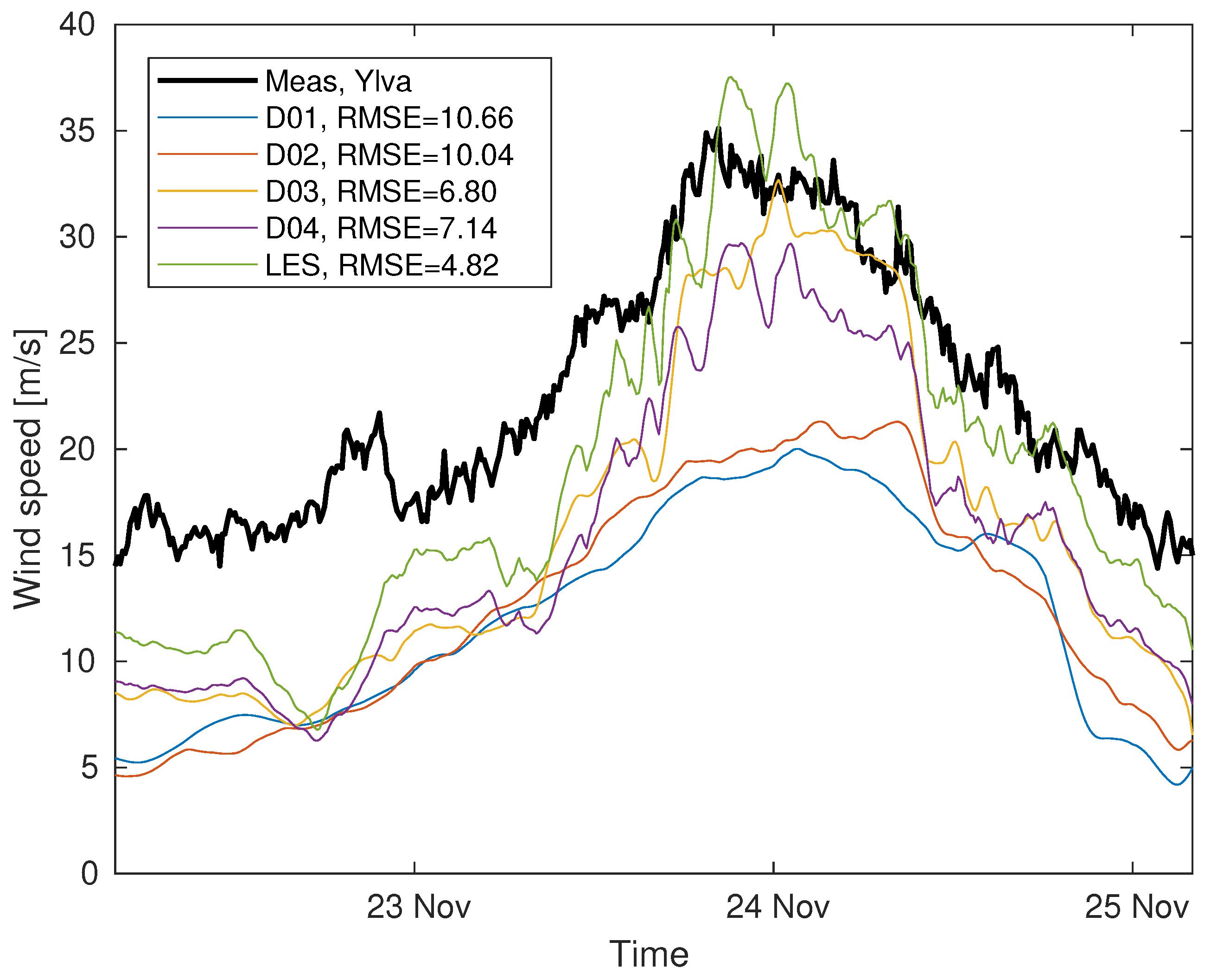
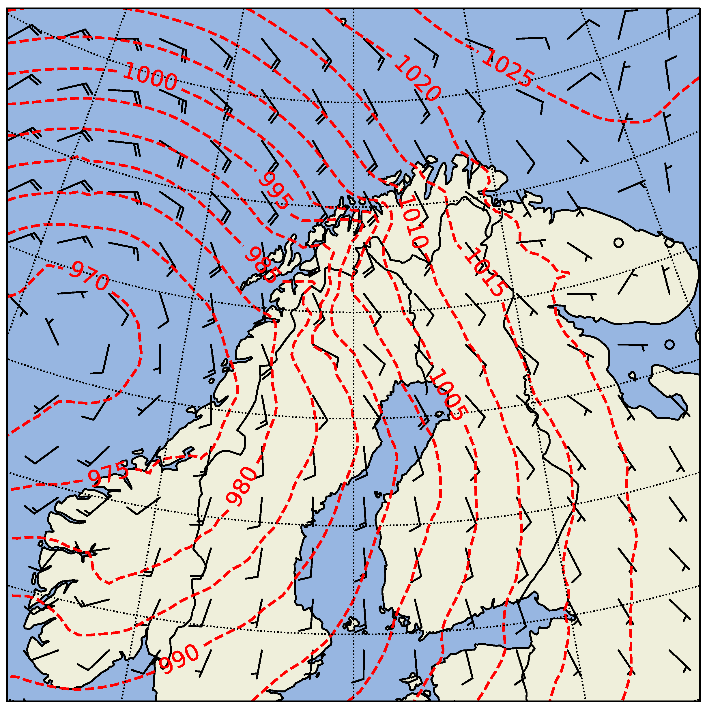
3.2. High-Wind Events

The measured wind speed and direction during 2017 are shown in the upper and lower parts of Figure 5a. The average wind speed was $\overline{w_s}=7.7$ m/s, with a seasonal variation given as $6.9,5.6,8.6$ and $9.6$ m/s for spring, summer, autumn and winter months, respectively. The 90th percentile wind speed, $w_s^{Q90}=14.2$ m/s, is shown as a red dashed line in the wind speed plot, and the ten longest events with wind speed above this percentile are the high-wind events that are coloured red in the measurement of both wind speed and direction. These events happened during the autumn and early winter season, and occurred with a wind direction of around 120°.

The histogram of the measured wind speed during 2017 is shown in Figure 5b, together with Rayleigh and Weibull distributions where the parameters are found using maximum likelihood estimates of the parameters. The histogram shows the highest frequency of wind speeds in the 6–7 m/s bin, where both the Rayleigh and Weibull distributions tend to underestimate the probability of these wind speeds. The histogram also has a slightly higher frequency of wind speeds when $w_s>15$ m/s, compared to the smoother estimated probability density functions.

The wind rose in Figure 5c confirms the tendency of the strongest winds coming from southeast (-east), but also shows that wind from either south or north-northwest was quite frequent this year. With almost no wind from either west or east, the wind blocking from the mountains in those directions is clearly shown in the wind rose. The wind rose also explains the overall location of wind turbines at Fakken, shown in Figure 1c, with two rows of turbines perpendicular to the main wind direction.

The 10 longest high-wind events are shown in Figure 6 as a function of the length of the event, with the starting time for each event shown in the plot legend. The longest event started on 22 November at 04:00, shown with a thin blue line, and lasted for 72 h. This event occurred during the strongest storm of the year named Ylva according to the Norwegian Meteorological office. During this storm, the measured wind speed, shown in the left plot in Figure 6, also surpassed 25 m/s for about 24 h, which typically is above the cut-off wind speed for wind turbines. The shortest duration of these events is the 9 November event that lasts for 12 h, and also note that the 21 November event (16+ h) is just before the Ylva storm event.

The wind direction in all events is around 120 degrees, as shown in the right plot of Figure 6, which confirms the tendency of southeast (east) wind as discussed for the wind rose for the whole year. Finally, the starting time of these events clearly shows that much of the strong wind occurred during the autumn and early winter season.

3.3. Modelled Wind Speeds During 2017

Table 1. Mean, STD, RMSE and R for measured and modelled wind speeds for the year 2017.

Time Series	Mean	STD	RMSE	R
Meas, 2017	7.69	4.62
WRF D01	7.89	4.07	4.22	0.54
WRF D02	7.41	3.79	3.92	0.58
WRF D03	7.17	3.55	3.40	0.69
WRF D04	7.23	3.53	3.74	0.68

shows the mean, STD, RMSE and R for the measured and modelled wind speed for 2017. The average wind speed from measurements was $7.69$ m/s, which is quite well represented by the WRF model, although D01 has a slightly higher value and D02–D04 slightly lower. The measured wind speed standard deviation is $4.62$, while the modelled wind speeds are in the $3.4$–$4.2$-range.

Comparing measured wind speed with WRF results, the results from WRF clearly show a lower RMSE and higher R as we increase the horizontal resolution of the model from 27 km to 3 km in D01 to D03, respectively. The innermost mesoscale simulation for D04 with a 1 km resolution has a slightly higher RMSE than D03, as well as a similar R. This result corresponds well with earlier results for this measurement site [27], where a 3 km resolution showed better agreement between the measurement and model than 1 km.

The normalised histograms for the measured and modelled wind speeds are shown in Figure 7. For wind speeds below the 90th percentile, the model values show a tendency towards higher wind speeds. This can clearly be seen as the probability density is shifted to higher wind speed in the model results. For wind speeds above the 90th percentile, on the other hand, the measured wind speeds have a tendency towards higher probability.

3.4. Strong-Wind Events

The 10 high-wind events identified in Figure 6 correspond to 19 daily simulations of the WRF model. The LES model uses the mesoscale model as input in a one-way nesting, and the WRF modelling is therefore rerun for these days, now with all five domains active.

The mean wind speed values during the strong-wind events shown in

Table 2. Mean, STD, RMSE and R for measured and modelled wind speeds for 10 strong-wind events during 2017.

Time Series	Mean	STD	RMSE [min, max]	R [min, max]
Meas, events	20.1	4.41
WRF D01	10.4	3.76	10.13 [9.81, 10.31]	0.78 [0.60, 0.81]
WRF D02	10.7	3.98	9.77 [9.39, 9.93]	0.78 [0.58, 0.81)
WRF D03	13.3	5.61	7.41 [7.18, 7.61]	0.86 [0.72, 0.89]
WRF D04	12.9	4.85	7.76 [7.55, 7.95]	0.82 [0.64, 0.85]
WRF LES	16.1	6.06	5.42 [5.20, 5.61]	0.80 [0.63, 0.85]

clearly show how WRF underestimates the wind speed for the low-resolution model. Increasing the resolution from D01 to LES does improve the wind speed results, but the mean wind speed is still clearly lower than the measured wind speed during these strong-wind events. The same tendency of improvement with higher-resolution models can be seen in STD and RMSE, while the correlation coefficient R clearly drops as resolution increases.

The statistical significance for RMSE and R was checked using the leave-one-out method, and the minimum and maximum of these statistics are included in Table 2. Assuming that the events are statistically independent, the low RMSE for LES is significantly lower than D03 and D04. A similar decrease in RMSE can be seen going from D01/D02 to D03/D04, while both pairs of domains have some overlap in their values. Regarding correlation, the D03 model has the highest R value, but the statistical spread is quite wide and overlapping for all model domains.

The measured wind speed during the Ylva storm event starting on 22 November is shown as the black line in Figure 8. The wind speed is around 15–20 m/s during the first 30 h, then it increases to 30–35 m/s before it slowly drops down again to the 90th percentile. The two WRF models with the lowest resolution have a wind speed that during the Ylva storm starts at 5 m/s, increases to approximately 18 m/s by 24 November, and then drops again to 5 m/s. The overall shape of the wind speed follows the measurement, but the wind speed is significantly lower in these WRF models. As we increase the resolution in the WRF model, the modelled wind speeds also increase. For the LES models, this means an overall shape that starts lower than the measurement at around 10 m/s as the start of the event, increases to the measured 30–35 m/s range during the most intense part of the storm, and follows the decreasing measured wind speeds quite well as the storm passes.

The legend in Figure 8 shows the RMSE values for the different model resolutions when only considering the Ylva storm event. The LES model can represent strong wind speeds during the event quite well and thus shows clearly lower RMSE results compared to the lower-resolution models. Increasing the resolution in the WRF models has a visible effect on the variability of the wind speeds, as the D01 result is quite smooth with slower variations than the high-resolution models. The high frequency variations in the LES model might explain the lower linear correlation to the measurements, since the timing for these variations does not necessarily match the measurements, although the standard deviations for these time series are similar.

Figure 9 shows the WRF model D01 sea level pressure on 23 November at 20:20, where the maximum wind speed of 35.1 m/s was measured, together with modelled wind speed barbs close to the surface indicating wind speed and direction. The synoptic situation during the Ylva storm event can be described by a strong low-pressure system (970 mbar) located in the Norwegian sea and a high-pressure system (1025 mbar) over the Kola peninsula to the east of North Norway [41]. The counterclockwise wind around the low-pressure system created strong wind from the southeast as the system moved north along the Norwegian coast.

Figure 10 shows the wind speed of 80 magl in D04 in two instances during the Ylva event, on 23 November at 00:00 and 20.20, respectively. The first instance is at the start of the event (Figure 10a), when the wind speed builds up at Fakken as the low-pressure systems come closer. The two large fjords south of Fakken are separated by the Lyngen Alps that direct the wind north on its eastern side, which then turns more easterly and against Fakken as it passes this mountain range. The next instance is in the middle of the storm (Figure 10b), when the measurements show the highest wind speeds. The overall wind direction has now turned slightly anticlockwise, but the fjords and mountains around Fakken make the wind direction at the measurement mast location very similar. The Lyngen Alps still lead some wind east of the mountain range in a northerly direction along the fjord, and a high-wind-speed location can be seen at the ocean in front of the Fakken wind park location. The complex terrain creates localised shadowing and tunnelling effects, and lee-side amplification indicates mountain waves in several places in the region, as also discussed in [27].

The wind speeds around Fakken for WRF D04 and WRF LES are shown in Figure 11, in the upper and lower rows, respectively. The upper left plot shows wind using WRF D04 on 23 November at 00:00, the same as in Figure 10a, but now zoomed in at Fakken wind park. The D04 results show a smooth wind field around Fakken wind park, with some blocking of wind in front of the mountain to the left of the wind park. The LES model, in the lower left plot, has higher wind speeds near the red circle that marks the location of the measurement mast, as well as reduced wind speeds in front of the low hill where the turbines are mounted. Closer to the mountains, the steeper terrain in the LES model also creates stronger shadowing effects, and we find indications of a mixed wind situation behind the mountain east of the mast. Turning to the right-hand plots, on 23 November at 20:20 in the middle of the storm, note that the wind speed colour range is now 0–52 m/s. The differences between D04 and LES are similar to those earlier in time. The terrain effects of blocking are much clearer in LESs compared to D04, and the speed increase along the low hills inside the Fakken wind park is clearly visible. The strong wind speed-up effects behind the eastern mountain are more distinct at this time, indicating lee wind behind this mountain.

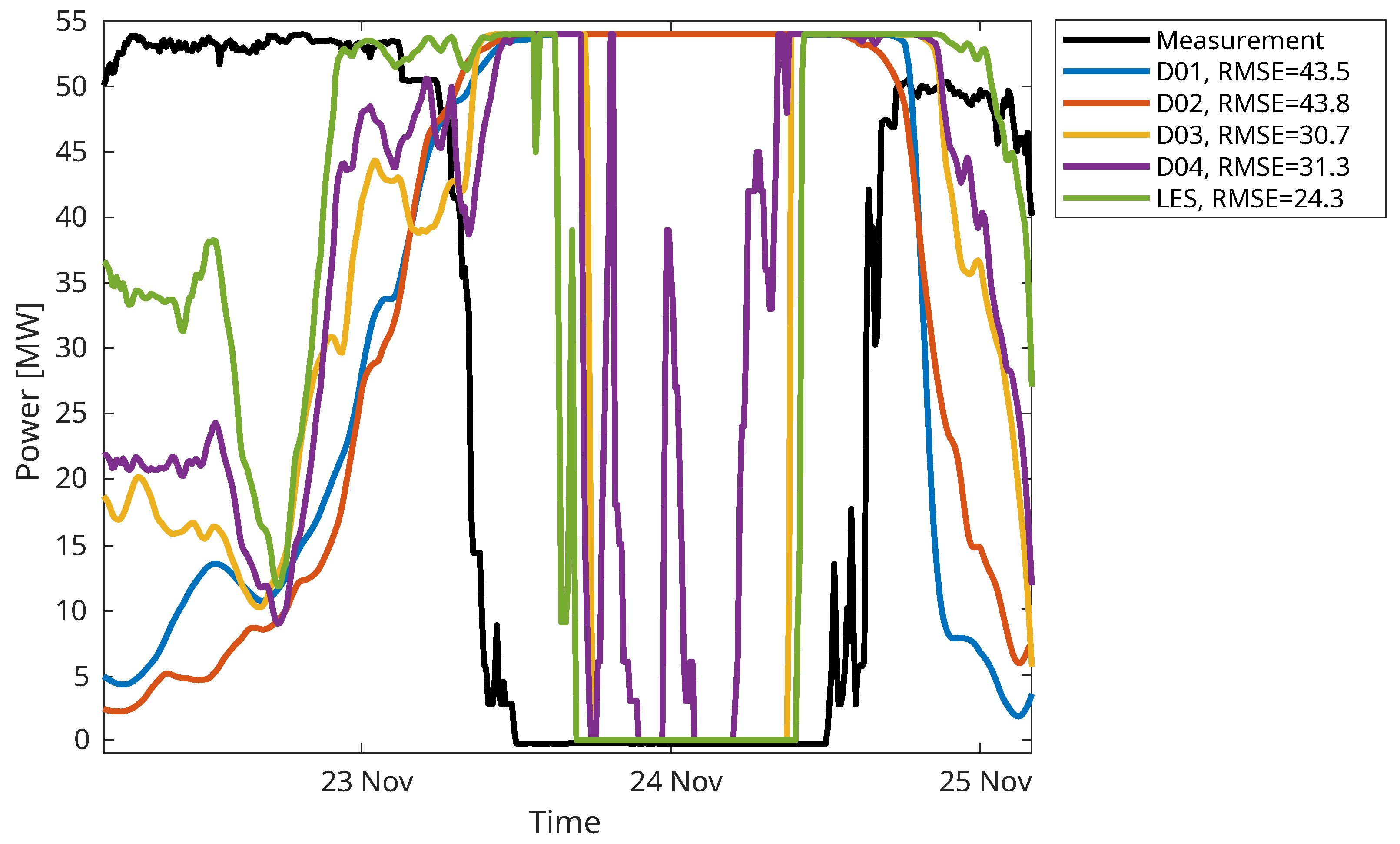
3.5. Wind Power Production

Strong winds can be complicated to handle for wind turbines, as the power curve typically drops rapidly from maximum to zero production as wind increases beyond the turbine cut-off wind speed $w_{cutoff}$ as discussed in Equation (2). In addition to the incoming mean wind speed, turbulence and rapid changes of wind direction introduce further challenges for wind turbine power production. In Figure 12, the total power production from the 18 wind turbines at Fakken is shown in the black line. During the start of the Ylva event, the measured wind is above the rated wind speed for the turbine and the production is around the installed power of 54 MW. During the morning of 23 November, the power production first dropped to around 50 MW before dropping rapidly to zero during the storm event. As the wind speed decreased on 24 November, the power production started up again and stabilised around 50 MW before a slight drop at the end of the high-wind-speed event. Note that the turbine control system is not connected to the wind speed at the measurement mast but instead uses measurements at the nacelles of each wind turbine in addition to possible other external sources.

Using the publicly available power curve of the Vestas V90 3 MW turbine, we have extracted the wind speeds from the WRF models at the location of each wind turbine, as shown in Figure 1c, and calculated the corresponding wind power production at Fakken wind park. The power production results of the different models are shown in Figure 12 together with their RMSE. As expected, the D01 and D02 models show very low power production during the start and end of the event, but also full production during the strongest part of the Ylva storm. This is a direct result of the underestimation of wind speed, as discussed earlier. The power productions using the D03 and D04 models are higher during the start and end of the storm event, and, in addition, they are also able to output zero production at times during the main storm event. Finally, the power production using WRF LES result shows clearly higher production during the start and the end of the event, and this method provides a longer period of zero production during the storm, although not as long as the measured production. The RMSE values summarise the overall model production, with LESs giving the lowest error, which was also seen for the RMSE of wind speeds in Figure 8.

4. Conclusions

The high-resolution WRF LES model can capture strong-wind events at Fakken wind park, although the WRF models in general tend to underestimate these high wind speeds. The complex terrain in the region, with several mountains and fjords, creates a challenging wind pattern as mesoscale systems move along the coast. The measured wind speed shows several strong-wind events during 2017, with the longest high-wind-speed events during the autumn and all coming from the south-southeast direction. The strongest event, the Ylva storm, recorded a continuous reading of more than 14 m/s wind speed over 72 h.

We have shown that the local terrain model improves considerably as the horizontal resolution is increased. This allows for more detailed wind patterns around the island where Fakken wind park is located, most visibly represented as higher and steeper mountains in the innermost domain of our simulations. Note that the use of high-resolution input data from NDTM with 10 m resolution is necessary for LES modelling, as results using LESs with GMTED and 30-arcsecond resolution do not reduce the underestimation of high wind speed compared to the D04 results.

The main reason for improved wind and power production estimates in the mesoscale models D01–D04 seems to be the models’ ability to create mountains and fjords that both block and channel the wind to this location. The highest resolution in the WRF LES model also provides refined terrain and wind fields, which produce local speed-up effects along the small narrow hill where both the measurement mast and the first rows of turbines at Fakken are located. Increasing the size of the LES domain would include more mountains and fjords, such as the Lyngen Alps, with the potential of increasing the tunnelling effect of the fjords.

Comparing measured power production with a basic turbine power modelling approach based on WRF wind speed, we have shown that the WRF LES gives noticeably better results during the Ylva storm event. This indicates that higher-resolution weather models may play an important role in the mapping of wind resources, as well as in wind power forecasting during storms and other extreme wind cases.

Although NWM using high-resolution LES mode can give a detailed description of the atmospheric conditions over a wind park without the need for local measurements, the use of WAsP and other specialised software for wind resources assessment plays an important role in the planning of a new wind park. These software solutions provide a generalised description of wind speed and direction with high horizontal resolution without a high computational cost. Turning the tables, WAsP does require trustworthy wind input data from a measurement mast, or well-defined WRF model outputs as in the New European Wind Atlas case [25]. The forecasting abilities in NWM are also useful for wind power forecasting applications, so that both solutions have their pros and cons in the future wind power industry.

This research is based on wind field results that are limited to one location and one year of data. The significantly lower RMSE in the LES modelling of the high-wind events is further based on the assumption that the events are statistically independent. This assumption can be misleading given such a limited dataset.

The LES model in our case has a single inner domain without sub-filter-scale stress, or SGS filters, a simplified setup that follows the real terrain well but has limitations when it comes to turbulence generation in the model. Future research should include SGS functions and wall functions to improve the turbulence structures in the model and better results along the domain borders. Further understanding of the underestimation of the high wind speeds, in storms and extreme weather, should include longer time series and locations with other wind climates including, for example, diurnal cycles or thermal winds. Future research could also include wind turbine parametrisations and the use of different PBL schemes for the driving outer domains.

References

1. Davenport, J.; Wayth, N. Statistical Review of World Energy; Energy Institute: London, UK, 2024; Available online: https://www.energyinst.org/__data/assets/pdf_file/0006/1542714/684_EI_Stat_Review_V16_DIGITAL.pdf (accessed on 5 June 2025).
2. GWEC. Global Wind Report 2025. Technical Report, Global Wind Energy Counsil. 2025. Available online: https://www.gwec.net/events/2025-global-wind-report-launch (accessed on 5 June 2025).
3. Ackermann, T.; Söder, L. An overview of wind energy-status 2002. Renew. Sustain. Energy Rev. 2002, 6, 67–127. [Google Scholar] [CrossRef]
4. Herbert, G.J.; Iniyan, S.; Sreevalsan, E.; Rajapandian, S. A review of wind energy technologies. Renew. Sustain. Energy Rev. 2007, 11, 1117–1145. [Google Scholar] [CrossRef]
5. Kwon, S.D. Uncertainty analysis of wind energy potential assessment. Appl. Energy 2010, 87, 856–865. [Google Scholar] [CrossRef]
6. Lars, L.; Lisbeth, M.; Ole, R.; Lundtang, P.E.; Hoffmann, J.B.; Jake, B.; Gylling, M.N. Wind Resource Estimation—An Overview. Wind Energy 2003, 6, 261–271. [Google Scholar] [CrossRef]
7. Burton, T.; Jenkins, N.; Sharpe, D.; Bossanyi, E. Wind Energy Handbook, 2nd ed.; John Wiley & Sons: Hoboken, NJ, USA, 2011; p. 780. [Google Scholar]
8. Byrkjedal, Ø.; Iversen, E.C.; Undheim, O. High resolution meso-scale calculations at two moderately complex sites. In Proceedings of the EWEA, Paris, France, 17–20 November 2015; p. 10. [Google Scholar]
9. Murthy, K.S.R.; Rahi, O.P. A comprehensive review of wind resource assessment. Renew. Sustain. Energy Rev. 2017, 72, 1320–1342. [Google Scholar] [CrossRef]
10. Al-Yahyai, S.; Charabi, Y.; Gastli, A. Review of the use of Numerical Weather Prediction (NWP) Models for wind energy assessment. Renew. Sustain. Energy Rev. 2010, 14, 3192–3198. [Google Scholar] [CrossRef]
11. Gastón, M.; Pascal, E.; Frías, L.; Martí, I.; Irigoyen, U.; Cantero, E.; Lozano, S.; Loureiro, Y. Wind resources map of Spain at mesoscale. Methodology and validation. In Proceedings of the European Wind Energy Conference and Exhibition 2008, Brussels, Belgium, 31 March–3 April 2008; Volume 5, pp. 2715–2724. [Google Scholar]
12. Tammelin, B.; Vihma, T.; Atlaskin, E.; Badger, J.; Fortelius, C.; Gregow, H.; Horttanainen, M.; Hyvönen, R.; Kilpinen, J.; Jenni, L.; et al. Production of the Finnish Wind Atlas. Wind Energy 2013, 16, 19–35. [Google Scholar] [CrossRef]
13. Kotroni, V.; Lagouvardos, K.; Lykoudis, S. High-resolution model-based wind atlas for Greece. Renew. Sustain. Energy Rev. 2014, 30, 479–489. [Google Scholar] [CrossRef]
14. Yu, W.; Benoit, R.; Girard, C.; Glazer, A.; Lemarquis, D.; Salmon, J.R.; Pinard, J.P. Wind Energy Simulation Toolkit (WEST): A Wind Mapping System for Use by the Wind-Energy Industry. Wind Eng. 2006, 30, 15–33. [Google Scholar] [CrossRef]
15. Gasset, N.; Landry, M.; Gagnon, Y. A Comparison of Wind Flow Models for Wind Resource Assessment in Wind Energy Applications. Energies 2012, 5, 4288–4322. [Google Scholar] [CrossRef]
16. Ermolenko, B.V.; Ermolenko, G.V.; Fetisova, Y.A.; Proskuryakova, L.N. Wind and solar PV technical potentials: Measurement methodology and assessments for Russia. Energy 2017, 137, 1001–1012. [Google Scholar] [CrossRef]
17. Jiménez, P.A.; González-Rouco, J.F.; García-Bustamante, E.; Navarro, J.; Montávez, J.P.; de Arellano, J.V.G.; Dudhia, J.; Muñoz-Roldan, A. Surface Wind Regionalization over Complex Terrain: Evaluation and Analysis of a High-Resolution WRF Simulation. J. Appl. Meteorol. Climatol. 2010, 49, 268–287. [Google Scholar] [CrossRef]
18. Carvalho, D.; Rocha, A.; Santos, C.S.; Pereira, R. Wind resource modelling in complex terrain using different mesoscale–microscale coupling techniques. Appl. Energy 2013, 108, 493–504. [Google Scholar] [CrossRef]
19. Tamura, T. Towards practical use of LES in wind engineering. J. Wind Eng. Ind. Aerodyn. 2008, 96, 1451–1471. [Google Scholar] [CrossRef]
20. Liu, Y.; Warner, T.; Liu, Y.; Vincent, C.; Wu, W.; Mahoney, B.; Swerdlin, S.; Parks, K.; Boehnert, J. Simultaneous nested modeling from the synoptic scale to the LES scale for wind energy applications. J. Wind. Eng. Ind. Aerodyn. 2011, 99, 308–319. [Google Scholar] [CrossRef]
21. Porté-Agel, F.; Wu, Y.T.; Lu, H.; Conzemius, R.J. Large-eddy simulation of atmospheric boundary layer flow through wind turbines and wind farms. J. Wind Eng. Ind. Aerodyn. 2011, 99, 154–168. [Google Scholar] [CrossRef]
22. Mehta, D.; van Zuijlen, A.; Koren, B.; Holierhoek, J.; Bijl, H. Large Eddy Simulation of wind farm aerodynamics: A review. J. Wind Eng. Ind. Aerodyn. 2014, 133, 1–17. [Google Scholar] [CrossRef]
23. Wise, A.S.; Neher, J.M.T.; Arthur, R.S.; Mirocha, J.D.; Lundquist, J.K.; Chow, F.K. Meso- to microscale modeling of atmospheric stability effects on wind turbine wake behavior in complex terrain. Wind Energy Sci. 2022, 7, 367–386. [Google Scholar] [CrossRef]
24. Fischereit, J.; Brown, R.; Larsén, X.G.; Badger, J.; Hawkes, G. Review of Mesoscale Wind-Farm Parametrizations and Their Applications. Bound.-Layer Meteorol. 2022, 182, 175–224. [Google Scholar] [CrossRef]
25. Dörenkämper, M.; Olsen, B.T.; Witha, B.; Hahmann, A.N.; Davis, N.N.; Barcons, J.; Ezber, Y.; García-Bustamante, E.; González-Rouco, J.F.; Navarro, J.; et al. The Making of the New European Wind Atlas—Part 2: Production and evaluation. Geosci. Model Dev. 2020, 13, 5079–5102. [Google Scholar] [CrossRef]
26. Fernández-González, S.; Martín, M.L.; García-Ortega, E.; Merino, A.; Lorenzana, J.; Sánchez, J.L.; Valero, F.; Rodrigo, J.S. Sensitivity Analysis of the WRF Model: Wind-Resource Assessment for Complex Terrain. J. Appl. Meteorol. Climatol 2018, 57, 733–753. [Google Scholar] [CrossRef]
27. Solbakken, K.; Birkelund, Y.; Samuelsen, E.M. Evaluation of surface wind using WRF in complex terrain: Atmospheric input data and grid spacing. Environ. Model. Softw. 2021, 145, 105182. [Google Scholar] [CrossRef]
28. Solbrekke, I.M.; Sorteberg, A.; Haakenstad, H. The 3 km Norwegian reanalysis (NORA3)—A validation of offshore wind resources in the North Sea and the Norwegian Sea. Wind. Energy Sci. 2021, 6, 1501–1519. [Google Scholar] [CrossRef]
29. Gandoin, R.; Garza, J. Underestimation of strong wind speeds offshore in ERA5: Evidence, discussion and correction. Wind Energy Sci. 2024, 9, 1727–1745. [Google Scholar] [CrossRef]
30. Powers, J.G.; Klemp, J.B.; Skamarock, W.C.; Davis, C.A.; Dudhia, J.; Gill, D.O.; Coen, J.L.; Gochis, D.J.; Ahmadov, R.; Peckham, S.E.; et al. The Weather Research and Forecasting Model: Overview, System Efforts, and Future Directions. Bull. Am. Meteorol. Soc. 2017, 98, 1717–1737. [Google Scholar] [CrossRef]
31. Lydia, M.; Kumar, S.S.; Selvakumar, A.I.; Prem Kumar, G.E. A comprehensive review on wind turbine power curve modeling techniques. Renew. Sustain. Energy Rev. 2014, 30, 452–460. [Google Scholar] [CrossRef]
32. Wang, Y.; Hu, Q.; Li, L.; Foley, A.M.; Srinivasan, D. Approaches to wind power curve modeling: A review and discussion. Renew. Sustain. Energy Rev. 2019, 116, 109422. [Google Scholar] [CrossRef]
33. Nakanishi, M.; Niino, H. Development of an Improved Turbulence Closure Model for the Atmospheric Boundary Layer. J. Meteorol. Soc. Jpn. Ser. II 2009, 87, 895–912. [Google Scholar] [CrossRef]
34. Thompson, G.; Field, P.R.; Rasmussen, R.M.; Hall, W.D. Explicit Forecasts of Winter Precipitation Using an Improved Bulk Microphysics Scheme. Part II: Implementation of a New Snow Parameterization. Mon. Weather Rev. 2008, 136, 5095–5115. [Google Scholar] [CrossRef]
35. Iacono, M.J.; Delamere, J.S.; Mlawer, E.J.; Shephard, M.W.; Clough, S.A.; Collins, W.D. Radiative forcing by long-lived greenhouse gases: Calculations with the AER radiative transfer models. J. Geophys. Res. Atmos. 2008, 113, 8. [Google Scholar] [CrossRef]
36. Mukul, T.; Chen, F.; Wang, W.; Dudhia, J.; LeMone, M.A.; Mitchell, K.E.; Ek, M.B.; Gayno, G.; Wegiel, J.W.; Cuenca, R. Implementation and verification of the unified Noah land-surface model in the WRF model. In Proceedings of the 20th Conference on Weather Analysis and Forecasting, Seattle, WA, USA, 10–15 January 2004; American Meteorology Society: Boston, MA, USA, 2004; p. 6. [Google Scholar]
37. Jiménez, P.A.; Dudhia, J.; González-Rouco, J.F.; Navarro, J.; Montávez, J.P.; García-Bustamante, E. A Revised Scheme for the WRF Surface Layer Formulation. Mon. Weather Rev. 2012, 140, 898–918. [Google Scholar] [CrossRef]
38. Kain, J.S. The Kain–Fritsch Convective Parameterization: An Update. J. Appl. Meteorol. 2004, 43, 170–181. [Google Scholar]
39. Wyngaard, J.C. Toward Numerical Modeling in the “Terra Incognita”. J. Atmos. Sci. 2004, 61, 1816–1826. [Google Scholar] [CrossRef]
40. Rai, R.K.; Berg, L.K.; Kosović, B.; Haupt, S.E.; Mirocha, J.D.; Ennis, B.L.; Draxl, C. Evaluation of the Impact of Horizontal Grid Spacing in Terra Incognita on Coupled Mesoscale–Microscale Simulations Using the WRF Framework. Mon. Weather Rev. 2019, 147, 1007–1027. [Google Scholar] [CrossRef]
41. Pedersen, I.T.; Vassbø, T.; Nordhagen, R.; Fossli, I.; Straume, I.; Mamen, J.; Haugen, G. Extream Weather Report; Technical Report; The Norwegian Meteorological Institute: Oslo, Norway, 2018. (In Norwegian) [Google Scholar]
Figure 1. Gray scale showing terrain height from Global Multi-resolution Terrain Elevation Data (GMTED) at 30-arcsecond resolution by United States Geological Survey. (a) Scandinavia peninsula. (b) Regional terrain. (c) Aerial photo using www.norgeskart.no (accessed on 1 March 2025). Red O: Location of measurement mast. Yellow letters: Location of wind turbines.
Applsci 15 07683 g001aApplsci 15 07683 g001b
Figure 2. WRF domain locations with colours showing model height data from 0 to 2000 m. White rectangles show borders between the nested domains.
Applsci 15 07683 g002
Figure 3. Terrain height in WRF domain D04 using Norwegian Digital Terrain Model with 10 m horizontal resolution. Black rectangular box corresponds to D05 LES domain.
Applsci 15 07683 g003
Figure 4. Terrain height zoomed in on the D05 location. Contour lines every 100 m, starting at 50 m. Red dot: Location of measurement mast. (a) Norwegian Digital Terrain Model, 10 m horizontal resolution. (b) WRF D03, 3 km resolution. (c) WRF D04, 1 km resolution. (d) WRF D05/LES, 90.9 m resolution.
Applsci 15 07683 g004
Figure 5. Wind measurements from Fakken wind power plant mast. (a) Wind speed (upper) and direction (lower). Red dashed line: 90th percentile value of the wind speed. Red values: The 10 longest durations above the 90th percentile. (b) Histogram with estimated probability density functions. (c) Wind rose showing speed and direction.
Applsci 15 07683 g005
Figure 6. Wind speed (left) and direction (right) of 10 longest high-wind events at Fakken wind park. Red dashed line: 90th percentage wind speed. Legend: Starting time of event.
Applsci 15 07683 g006
Figure 7. Normalised histograms for measured and modelled wind speeds for the year 2017.
Applsci 15 07683 g007
Figure 8. Measured and modelled wind speeds during Ylva storm. RMSE for this event is shown in legend for each model.
Applsci 15 07683 g008
Figure 9. Surface-level pressure in WRF D01 23 November at 20:20 shown as red dashed contour lines. Wind barbs from lowest model level.
Applsci 15 07683 g009
Figure 10. Wind speed and wind barbs at 80 magl from WRF D04. Red dot: Location of measurement mast. Colour: Wind speed; note different scales. Contour lines every 200 m, starting at sea level.
Applsci 15 07683 g010
Figure 11. Wind at 80 magl from WRF D04 (upper row) and WRF LES (lower row). Red circle: Location of measurement mast. Left plots: 23 November at 00:00; right plots: 23 November at 20:20. Contour lines every 100 m, starting at 50 masl.
Applsci 15 07683 g011
Figure 12. Measured and modelled power production during the Ylva storm together with their corresponding RMSE.
Applsci 15 07683 g012