Enhancing Power Converter Reliability Through a Logistic Regression-Based Non-Invasive Fault Diagnosis Technique

Abstract

Sustainability can be achieved through the widespread adoption of electrification across multiple sectors of activity, which would thereby enable increased operational efficiency and reduce the environmental impact. The attainment of this purpose relies on electrical circuits that convert electrical energy from renewable power plants into forms that are compatible with the specific requirements of the load. Failure of the aforementioned circuits, denominated as power converters, can lead to financial losses resulting from unexpected shutdowns and, in critical systems, can pose significant risks to human life. This article focuses on the topic of fault diagnosis in power converters. Some of the most vulnerable components of these converters are the capacitors used in the DC-link, whose failure evolves gradually. When the capacitor internal resistance (ESR) or the capacitor capacitance (C) exceeds a certain threshold value, it is advisable to propose a system shutdown, as soon as possible, to replace the capacitor. The solution presented in this article combines signal processing techniques (SPTs) with a machine learning (ML) algorithm to determine the optimal time for capacitor replacement. The ML algorithm employed herein was a logistic regression (LR) algorithm which classified the capacitor into one of two states: normal operation (0) or failure (1). To train and evaluate the LR model, two different datasets were created using various electrical quantities that can be measured non-invasively. The model demonstrated excellent performance, achieving an accuracy, precision, recall, and F1 score above 0.99.

1. Introduction

Reducing greenhouse gas emissions has become a global priority, which has made it imperative to increasingly use clean energy sources, particularly renewable energy sources. Therefore, phasing out oil and its derivatives is now a key objective of greenhouse gas reduction. In the European Union, in 2022, electricity was the second largest energy vector after oil and its derivatives, representing a share of the total final energy consumption of 23% [1]. On the other hand, the International Energy Agency’s Electricity 2024 report indicates that the share of electricity in final energy consumption increased from 18% in 2015 to 20% in 2023 [2]. This reflects a broader global shift toward electrification and sustainable energy use.

This paradigm shift is impacting all sectors of the economy. For instance, in the primary sector, in agriculture and fishing, there is an increasingly broad integration of hybrid and electric vehicles [3], robots, and drones [4,5], which increase the operational efficiency and reduce the environmental impact of these sectors. In turn, in the secondary sector, industrial electrification represents an irreversible trend [6] which not only optimizes energy efficiency but also guarantees a substantial reduction in greenhouse gas emissions. Finally, the tertiary sector is also witnessing an unprecedented transformation, which is marked by the increasing use of electric vehicles in public transport systems [7,8] and the adoption of advanced, energy-efficient electrical equipment in sectors such as healthcare [9] and commerce [10].

Electrification relies on electrical circuits that convert grid-supplied waveforms into forms that are compatible with the specific requirements of each load. In this context, power electronics plays a crucial role by enabling the design of power converters (PCs) that efficiently transfer energy from one form (source) to another (load).

Failures in power converters cause significant financial losses resulting from unexpected shutdowns [11]. On the other hand, in critical systems, these failures pose serious risks to human life, notably when they effect medical equipment and transport vehicles, where converters are vital to ensure the reliable operation of essential functions [12].

PCs typically consist of switches, lossless energy storage elements, and magnetic components such as transformers. Among these, capacitors, a key energy storage device, are particularly vulnerable and are responsible for approximately 30% of all PC failures [13]. Capacitor failures typically advance gradually but can lead to catastrophic outcomes if not addressed promptly. As a result, designing real-time fault diagnosis techniques (FDT) to monitor the health status of capacitors has become essential. This topic has gained significant attention in recent years due to increasing electrification, although initial research efforts date back more than two decades ago [14].

FDTs can be classified from both operational and conceptual perspectives. From the operational standpoint, FDTs are typically divided into offline (OFF), quasi-online (QON), and online (ON). Offline fault diagnosis techniques (OFF-FDTs) involve removing the capacitor from its original circuit (the PC) and testing it separately in a dedicated setup. While this approach can yield highly accurate results [15], it is generally impractical because it requires shutting down the PC and physically removing the capacitor from the PC. In quasi-online fault diagnosis techniques (QON-FDTs), the capacitor is not removed from the PC, and its health status is assessed during a routine PC interruption. The routine interruption may represent an atypical converter operation or special operating configuration [16]. Online fault diagnosis techniques (ON-FDTs) can be implemented during normal converter operation; thus, the capacitor’s health status can be assessed constantly and uninterruptedly, which ensures that there are no interruptions or the need for the introduction of atypical operating conditions. This makes the ON-FDT an ideal solution for implementing predictive maintenance strategies [14,17].

Since the goal is to design a solution suitable for predictive maintenance, this paper will focus exclusively on ON-FDTs, which can be conceptually classified into three categories: signal-based (SB), model-based (MB), and data-based (DB) [17].

Signal-based online fault diagnosis techniques (SB-ON-FDTs) assesses the health status of capacitors by analyzing the analytical relationships between features extracted from measured signals. These features can be obtained using time-domain methods, frequency-domain methods, or hybrid approaches [18,19]. SB-ON-FDTs offer a fast response and do not require prior knowledge of PC parameters or large datasets for model training. However, they rely on additional sensors, are typically invasive in nature, and may produce false fault alarms when the PC is operating under extremely dynamic conditions [20,21].

Model-based online fault diagnosis techniques (MB-ON-FDTs) rely on the converter’s model, which represents a mathematical representation of the system’s expected behavior. A fault may be acknowledged when there is a discrepancy between the model output and the actual data from the physical system. Unlike the previous approach, MB-ON-FDTs are model-dependent and require a deep understanding of the system’s underlying model [13].

Data-based online fault diagnosis techniques (DB-ON-FDTs) evaluate the capacitor’s health status by directly analyzing real-world data. However, this approach requires a training dataset to enable the machine learning (ML) model to learn how to identify faults [17].

This paper proposes a solution that aims to overcome some of the identified constraints, which will be detailed and discussed in Section 4 and Section 5. Section 2 will focus on aluminum electrolytic capacitors (al-caps), a common technology used in the design of PCs. A brief overview of the current state of the art of FDTs in PCs will be provided in Section 3. In Section 6 and Section 7, the proposed method is evaluated on an entirely new dataset to demonstrate its effectiveness and adaptability across different scenarios. Finally, Section 8 will summarize the main conclusions.

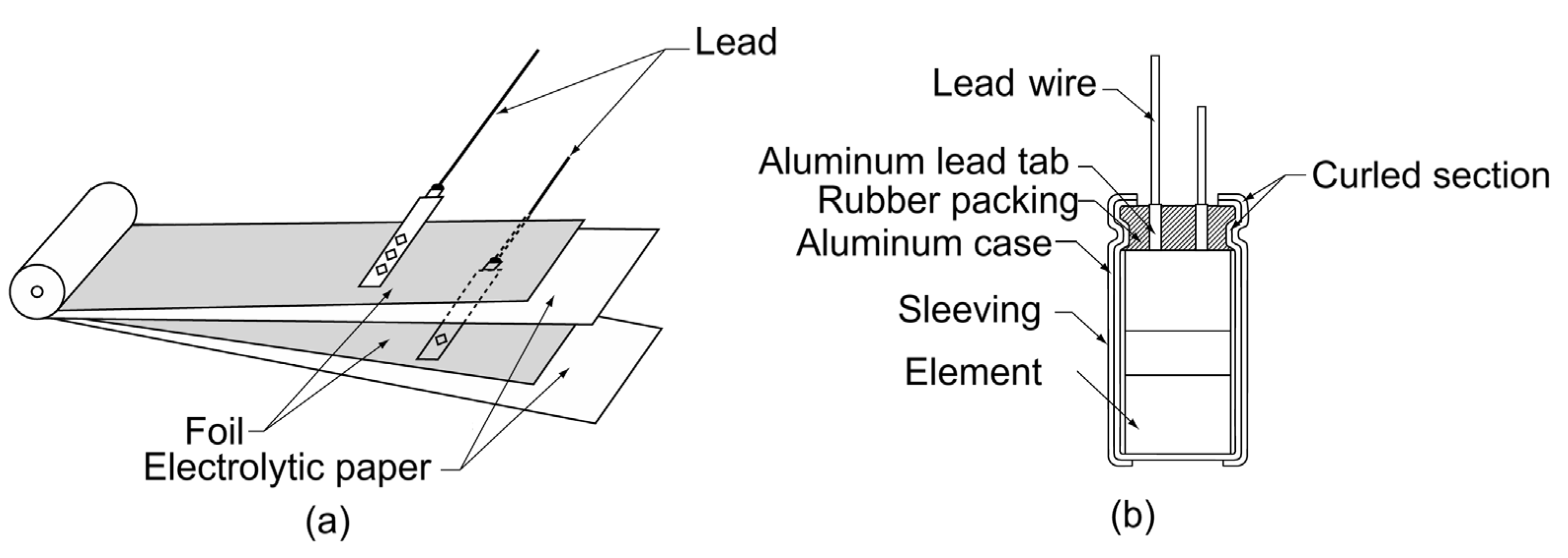
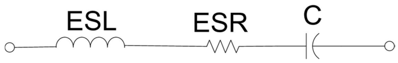
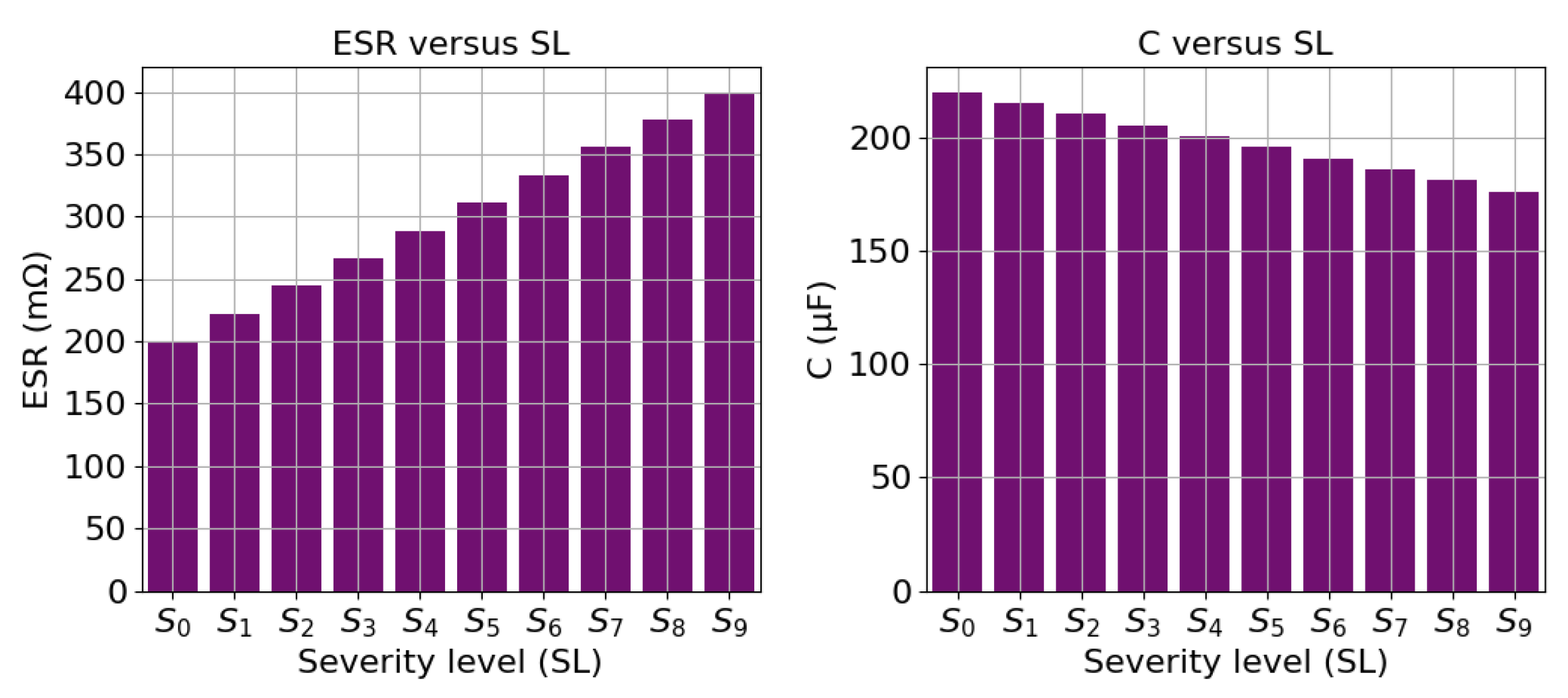
2. Aluminum Electrolytic Capacitors (Al-Caps)

Capacitors are generally classified into three main types: electrolytic, film, and ceramic. Each type can be further subdivided based on factors such as the dielectric material, construction, terminal connection, application, coating, and electrolyte that are used [14].

Among the capacitors used in PCs, aluminum electrolytic capacitors (al-caps) are widely used because they have high volumetric efficiency, are compact, are cheap, and are available in a wide range of capacitance values [22,23]. However, their high dissipation factor and leakage current limit their maximum operating voltage to about 1 kV [24].

Al-caps consist of a wound element (Figure 1a) that is impregnated with an electrolyte, connected to the leads, and placed inside a metal can (Figure 1b). The element itself is composed of two aluminum foils, the anode and cathode foil, which are physically separated by paper separators soaked in electrolyte (Figure 1a).

The foils are composed of high-purity aluminum and are etched with billions of microscopic tunnels, which significantly enhances their surface area [14,22,23].

Internally, an al-cap consists of two capacitors: the anode capacitor (an-al-cap) and the cathode capacitor (ca-al-cap). The an-al-cap comprises an anode foil (positive plate), a dielectric layer (designed to withstand the rated voltage), and the electrolyte (serving as the negative plate). The ca-al-cap, on the other hand, consists of the electrolyte (positive plate), a much thinner dielectric layer (supporting voltages below 0.5 V), and the cathode foil (negative plate) [14].

The electrolyte, which serves as the cathode for the an-al-cap, is an ion-conducting liquid that comes into contact with the dielectric layer, the aluminum oxide (Al₂O₃). Its main functions are to ensure firm adhesion to the surfaces of both foils, establish electrical continuity between the an-al-cap and ca-al-cap, and assist in repairing defects in the anode dielectric layer. The strong adhesion of the electrolyte to the aluminum foil maximizes the contact area, thereby increasing the al-cap capacitance. When defects form in the dielectric layer, the leakage current increases, triggering the electrolysis of the water in the electrolyte and generating hydrogen and oxygen. The released oxygen then reacts with the anode foil, regenerating Al₂O₃ in areas where the dielectric layer is thinner or damaged.

The process described above is known as the self-healing mechanism, and it naturally changes the electrical characteristics of the al-cap. As the water content in the electrolyte decreases, the contact area with the dielectric layer is reduced, which leads to a drop in capacitance. Additionally, the reduction in the electrolyte impairs the electrical connection between the an-al-cap and the ca-al-cap, which results in an increase in the capacitor’s internal resistance. Another important aspect to consider is the generation of gases, which increases the internal pressure within the can. To prevent rupture or explosion, the capacitor is equipped with a pressure-relief mechanism designed to safely release excess pressure.

The equivalent circuit of an al-cap (Figure 2) can be modeled using three main components: an ideal capacitor (C), the equivalent series resistance (ESR), and the equivalent series inductance (ESL).

The ESR accounts for various resistive elements within the capacitor, including terminal, tab, and foil resistances, as well as the paper–electrolyte and tunnel–electrolyte resistances. It also includes the parallel resistance associated with the leakage current. The ESL arises from the tab loop configuration, specifically the loop area formed by the terminals and tabs outside the active winding [14].

Failures in aluminum electrolytic capacitors (al-caps) can have several causes, but the two main mechanisms are the self-healing mechanism, described above, and electrolyte evaporation. The latter occurs due to high operating temperatures and high ripple currents leading to gradual loss of the electrolyte solution [25].

Having examined the composition, equivalent circuit, and primary failure mechanisms of al-caps, it is now possible to understand how aging alters the capacitor equivalent circuit. Since one of the primary failure mechanisms involves electrolyte loss, the main consequences of failure are an increase in the ESR and a decrease in the C. This aging process occurs gradually, becoming more pronounced as the electrolyte evaporates. Over time, the diminishing electrolyte weakens the connection between the an-al-cap and the ca-al-cap, eventually leading to complete failure of the al-cap (open-circuit). To prevent catastrophic failures like open circuits, which can severely degrade converter performance, manufacturers establish threshold values for the ESR and C of al-caps. Once these thresholds are reached, corrective action should be taken to replace the al-caps in a PC. These thresholds typically correspond to a 100% increase in the ESR and a 20% decrease in capacitance [26].

3. Cutting-Edge Online Fault Diagnosis Techniques for Al-Caps

An overview of ON-FDTs implemented in various PC topologies to evaluate the health conditions of capacitors is provided in this section.

3.1. Signal-Based Online Fault Diagnosis Techniques (SB-ON-FDTs)

In [27], the authors introduced an SB-ON-FDT to assess the condition of the al-cap used in the output filter of a forward converter. They established an analytical relationship between two features, of the capacitor’s voltage ripple and current ripple signals, namely, the peak-to-peak values of these waveforms. It was later demonstrated that the previous analytical relationship could be equally applied to buck-type converters operating in both continuous conduction mode (CCM) and discontinuous conduction mode (DCM) [28]. It is important, however, to emphasize that the previous relationship is only valid in a steady state regime, which means that load variations are not considered. Later, in [29], the authors proposed an SB-ON-FDT for boost and buck-boost converters, based on a novel analytical relationship between the output voltage ripple and the input current. The key advantage of this approach is that it eliminates the need for a current sensor in the capacitor branch. In [30], the authors present an analytical relationship between the average power dissipated by the capacitor and the root mean square (RMS) value of its current to estimate the ESR. This solution was integrated into a pulse-width modulation (PWM) adjustable speed drive (ASD). The methods outlined above first extract features from the signals using time-domain techniques. Afterwards, a straightforward analytical relationship is used to estimate the ESR value and, finally, using the ESR value, it is possible to evaluate the al-cap’s condition.

The approaches described below can be also categorized as SB-ON-FDTs. However, instead of applying time-domain techniques to extract signal features, they employ frequency-domain techniques. In [31], the authors present a solution for estimating the ESR value based on a simple relationship between the fundamental components of the capacitor’s voltage and those of its current. To implement this solution, an intelligent, cost-effective, and straightforward electronic module was designed for a DC-DC forward converter which provides an alert when the al-cap needs replacement. Specifically, when the estimated ESR value exceeds twice that of a sound capacitor, replacement is advised. Subsequently, the same principle was applied to an ATX power supply to assess primary side condition of al-caps [32]. Unlike the solution proposed in [31], which combines a bandpass filter with a (root mean square) RMS to DC converter to estimate the ESR, in [32], the discrete Fourier transform (DFT) algorithm is used to estimate the ESR at the converter’s switching frequency. Subsequently, in [33], the Goertzel algorithm is applied to the DC-link capacitors used in front-end rectifier-fed three-phase inverters to extract the waveform characteristics of the capacitor’s current and voltage. Following this, using two analytical relationships between signal features, it is possible to estimate both the ESR and C. In [19], the authors combine the discrete wavelet transform (DWT) with an RMS filter and a Kalman filter to estimate the both the ESR and C values of the al-cap used in the output filter of a three-phase interleaved boost converter (3ϕIBC). Subsequently, in [34], the ESR value is estimated by combining the Hilbert transform with two filters: an RMS and an average filter. This approach eliminates the need for a dedicated current sensor in the capacitor branch, as it uses the inductor currents that are required for 3ϕIBC control. In [35], the authors also use the inductor current and output voltage ripple to estimate the ESR. After acquiring the signals from a buck converter, they apply empirical mode decomposition (EMD) followed by the Hilbert–Huang transform (HHT) to extract the signal’s modes, from which the ESR value is estimated. Although the last two techniques are not entirely non-invasive, they impose fewer practical constraints compared to methods that require inserting a current sensor into the capacitor branch. In [36], the authors apply a bandpass filter to extract the AC components of the DC-link voltage and current in an uninterrupted power supply (UPS). By analyzing the modes of these signals, they calculate the power loss in the aluminum capacitor (al-cap) and estimate its equivalent series resistance (ESR). To overcome the practical limitations of placing a current sensor in the capacitor branch, the current in the capacitor is reconstructed using the output current of the rectifier, the current to the inverter, and the current to the battery module.

In [37], the authors propose a method to estimate the ESR values of al-caps used in the output filters of boost converters by analyzing the inductor current and the output voltage waveforms. First, they apply an analog high-pass filter combined with a wavelet transform denoising (WTD) method to extract the ripple from the output voltage. Then, using the output voltage ripple, the inductor current, and a set of analytical expressions, they estimate the ESR value. This approach integrates time-domain and frequency-domain techniques, and is thus a hybrid method.

3.2. Model-Based Online Fault Diagnosis Techniques (MB-ON-FDTs)

Model-based online fault detection techniques (MB-ON-FDTs) rely on the physical system model to which they are applied, which makes them well-suited for PCs, as these hybrid dynamical systems can be effectively described using state-space models. Therefore, in [38], the authors apply the recursive least mean squares (RLMS) algorithm to identify the coefficients of the state space model of a buck converter, which naturally includes the capacitor parameters. Later, in [39], a simplified regression model for buck and boost converters was proposed that reduced both the computational cost and time required for calculations. Although accurate, the two previous methodologies require a high sampling frequency. To address this issue, in [40], a continuous-time model of the buck converter was used in conjunction with the LMS algorithm to estimate the ESR value. This approach focuses solely on the non-conduction stage of the buck converter. Subsequently, the previous solution was adapted for buck-boost and boost converters [41]. However, as the two previous solutions use samples associated with a specific converter state, the size of the duty cycle may restrict their implementation. Thus, in [42], a unified method is proposed for three non-isolated converters: buck, buck-boost, and boost converters. This new method uses samples from the converter state that has the largest number of samples available. Subsequently, the concept of a digital twin is introduced and applied to assess the health status of the capacitors used in the output filter of a buck converter [43]. Using the circuit model, the authors employ the particle swarm optimization (PSO) algorithm to estimate the main circuit parameters, namely the C and ESR, by minimizing the discrepancy between the digital twin and the physical system.

3.3. Data-Based Online Fault Diagnosis Techniques (MB-ON-FDTs)

Data-based online fault diagnosis techniques (DB-ON-FDTs) can be classified into two categories: deep learning DB-ON-FDTs (DL-DB-ON-FDTs) and traditional ML DB-ON-FDTs (TML-DB-ON-FDTs). The DL-DB-ON-FDTs require a very substantial volume of training data, for which some solutions will be presented below. Although DL algorithms are capable of operating directly on raw data, the following solutions require data pre-processing. Consequently, it is essential to extract specific features from the sampled signals prior to model training. The first approaches address the problem as a regression task, wherein the dependent variable corresponds to the capacitor capacitance value. The first solution proposes the implementation of an artificial neural network (ANN) to estimate the DC-link capacitor capacitance in a back-to-back converter [44]. The features correspond to the RMS values of the input and output voltage and current of phase A together with DC-link voltage, with the C value being the target. Subsequently, in [45], the number of inputs to the ANN is reduced to two, namely the RMS value of a single-phase output current and the voltage ripple across the DC-link. In [46], the authors propose a feature set comprising a combination of DC-link voltage harmonics. In [47], an adaptive neuro-fuzzy inference system (ANFIS) is employed to evaluate the condition of the capacitors within a wind power system supplying a single-phase electrical grid. One capacitor is positioned at the output of the three-phase rectifier, while the other is situated between the boost converter and the input of the single-phase inverter. The input features for the ANFIS model include the converter’s input voltage and the voltages across the terminals of both capacitors. Unlike the previously discussed approaches, which address the problem as a regression task, this method formulates it as a classification problem. Accordingly, the ANFIS output identifies one of three possible states: normal operation, failure of the first capacitor, or failure of the second capacitor. Subsequently, in [17], the authors employ an autoencoder trained exclusively on data from a healthy 3ϕIBC, which enables the accurate reconstruction of the input signal under healthy conditions. As expected, the reconstruction error remains low in healthy scenarios; however, when the autoencoder processes input data from a system with aged capacitors, the reconstruction error increases significantly, thereby enabling fault detection. The inputs to the autoencoder include the output voltage amplitude, which are extracted using the short-time least squares Prony (STLSP) algorithm, the load resistance, and the average output voltage. Although the autoencoder is provided with three inputs, it produces a single output: the reconstructed amplitude of the output voltage. The other two inputs play a crucial role in enabling the autoencoder to identify the operational state of the converter. Deviations in the reconstruction error serve as a reliable indicator of the capacitor’s health status. Recently, in [48], the authors introduced a new DL-DB-ON-FDT that uses raw data as its input, specifically the voltage across the DC-link capacitor of a three-phase PWM inverter for induction motor drives. To estimate both the ESR and C values of capacitors, a hybrid convolutional neural network (HCNN) with an attention mechanism is employed.

Alongside DL-based solutions, there are also TML-DB-ON-FDTs, which will be discussed below. In [49], traditional ML algorithms such as the K-nearest neighbors (KNN), support vector machine (SVM), and naive Bayes (NB) algorithms are used to monitor the condition of a DC-link capacitor in a back-to-back (BTB) converter. Prior to training the models, features are extracted from the raw signal (the DC-link voltage) using wavelet decomposition. Therefore, the kurtosis, skewness, standard deviation (STD), root mean square (RMS), energy entropy (EE), and crest factor (CF) are extracted from the fourth wavelet coefficient. The authors frame the problem as a classification task, with the models being trained to distinguish between five states: healthy, aged, critical, very critical, and high alarm. In [50], the authors propose a method that integrates a SVM classifier with time-frequency analysis of conducted EMI to assess the condition of DC-link capacitors in a three-phase inverter. The EMI signals are analyzed during switching events using the continuous wavelet transform (CWT), which generates distinctive switching patterns. An analytic Morse wavelet is used for the analysis, and is configured with a symmetry parameter of 3, a time-bandwidth product of 60, and 10 voices per octave. The extracted patterns serve as input features for training a SVM classifier, which enables it to categorize the capacitor’s condition into five severity levels. In [51], the authors propose a random forest classifier (RFC) that triggers an alert when the ESR of the output filter capacitor in a boost converter exceeds a predefined threshold. The input features include the capacitor voltage amplitude at the converter switching frequency, extracted using the STLSP algorithm, along with the load resistance and duty cycle. The RFC is trained to classify the condition as either a healthy al-cap or an aged al-cap. In [52], the authors use a logistic regression (LR) model to assess the condition of the output filter capacitor in a 3ϕIBC. The capacitor current is reconstructed using the control signal and inductor currents. The raw data are processed through a bank of four filters to isolate the four most significant spectral components. Features are then extracted from these components using an RMS filter. Finally, these features are fed into the LR model, which, after training, classifies the capacitor as either a healthy al-cap or an aged al-cap.

3.4. Comparing Online Fault Diagnosis Methods

Most SB-ON-FDTs are invasive, as they rely on current sensors. Further, many of these techniques depend on a sensor in the capacitor branch, which makes them impractical for real-world applications due to space constraints and potential operational limitations.

MB-ON-FDTs generally require high sampling frequencies and involve complex models, which can vary depending on the converter topology. Additionally, MB-ON-FDTs typically demand access to the converter internal state variables, which makes these approaches intrinsically invasive by nature.

On the other hand, DB-ON-FDTs, particularly those based on deep learning, offer excellent performance but come with significant drawbacks. They require large training datasets and substantial computational resources, which poses a considerable challenge to their integration into commercial systems. It is worth noting that the aforementioned issue related to the generation of large datasets can be substantially mitigated by implementing the proposed approach, which simply involves adapting the pipeline to accommodate a deep learning model.

This paper presents an innovative solution to address these aforementioned limitations by integrating signal processing techniques (SPTs) with traditional machine learning algorithms (TMLs) in order to evaluate the state of capacitors used in the DC-link of PCs. Although TML models require preliminary data preprocessing, they offer substantial advantages over deep learning approaches, including the ability to learn effectively from significantly smaller training datasets with a lower computational cost. Furthermore, in contrast to SB-ON-FDTs and MB-ON-FDTs, TML-DB-ON-FDTs enable the implementation of non-invasive and efficient FDTs using features derived from the converter input and output signals, eliminating the need for integrating internal sensors into the converter system.

Specifically, a logistic regression (LR) model is used to evaluate the health status of an al-cap used in the output filter of a buck converter. The proposed methodology only uses the input and output currents of the converter, together with the output voltage, thus constituting a non-invasive approach. The proposed solution has a minimal computational cost, which occurs exclusively during the training phase, since the LR generates a mathematical equation and a decision criterion that allows the evaluation of the capacitor condition. Once the equation and decision criterion are established, implementing this solution requires minimal computational resources and can be readily integrated into microcontroller-based systems.

The development of the proposed FDT seeks to provide a computationally efficient, non-invasive, and scalable solution that is well-suited for practical implementation in real-world applications.

4. Proposed Online Fault Diagnosis Technique for Al-Caps Using Traditional Machine Learning Algorithms

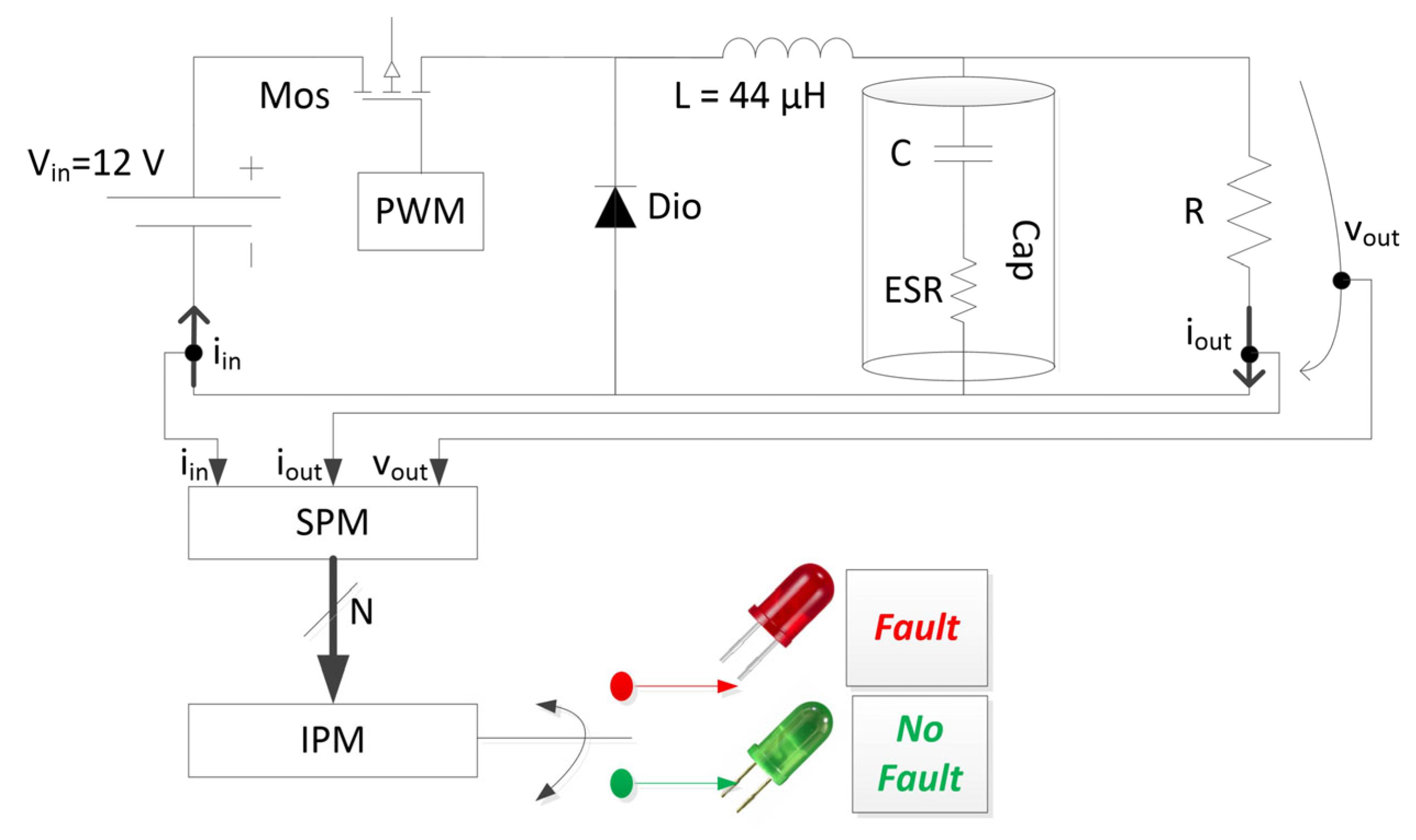
This paper proposes a traditional machine learning data-based online fault diagnosis technique (TML-DB-ON-FDT) that relies solely on input and output signal measurements, eliminating the need for internal sensors within the converter and ensuring independence from the converter model. The method employs logistic regression (LR), a lightweight ML algorithm that requires far less data than artificial neural networks (ANNs), to learn patterns and detect when capacitor replacement is necessary. Once trained, the FDT model is represented as a simple mathematical equation combined with a condition, which makes it highly efficient and significantly reduces the computational cost and processing time compared to alternative approaches.

Traditional ML algorithms cannot operate directly on raw data, requiring prior feature extraction from the given raw data. Therefore, as the ML algorithm used is LR, it is necessary to first extract features from the raw data. Thus, the proposed solution is composed of two fundamental components: the signal processing module (SPM) and the information processing module (IPM). In the SPM, the raw data are converted into meaningful primary features. In the IPM, the primary features are used to assess the al-cap’s health status.

This section introduces the converter under analysis, the SPM, and the complete pipeline used to generate the datasets for training and testing the LR model. The IPM will be discussed in Section 5.

4.1. Buck Converter

A buck converter was employed to validate the proposed TML-DB-ON-FDT due to its wide use and high efficiency in reducing the input voltage [53]. This topology is well suited for applications that require low voltages and high output currents, such as DC power networks and microgrids [54], photovoltaic (PV) systems [55], electric vehicles (EVs) battery chargers [56], internet of things (IoT) applications [57], and implantable medical devices (IMDs) with wireless power transfer (WPT) [58], among others.

Figure 3 illustrates the schematics of a buck converter, which includes two semiconductor devices, a diode (Dio) and a transistor (Mos) that regulate the current flow along with two energy storage elements, an inductor (L), and a capacitor (Cap) that stores energy temporarily. In the conducting state, the Mos is ON and the Dio is OFF. During this phase, current flows through the inductor (L) and the capacitor (Cap), with both storing energy, and also passes through the load resistor (R). In the non-conducting state, the Mos turns OFF, causing the Dio to conduct. Therefore, the current flows through the L, Cap, Dio, and R.

Figure 3 displays the raw data, which include the converter input and output currents (i_in and i_out), the output voltage (v_out), the SPM, the IPM, and the alarm mechanism. Initially, the SPM processes the raw data into N primary features, which are then analyzed by the IPM to assess the condition of the al-cap. If the capacitor is in good health, the green LED is activated; otherwise, the red LED turns ON.

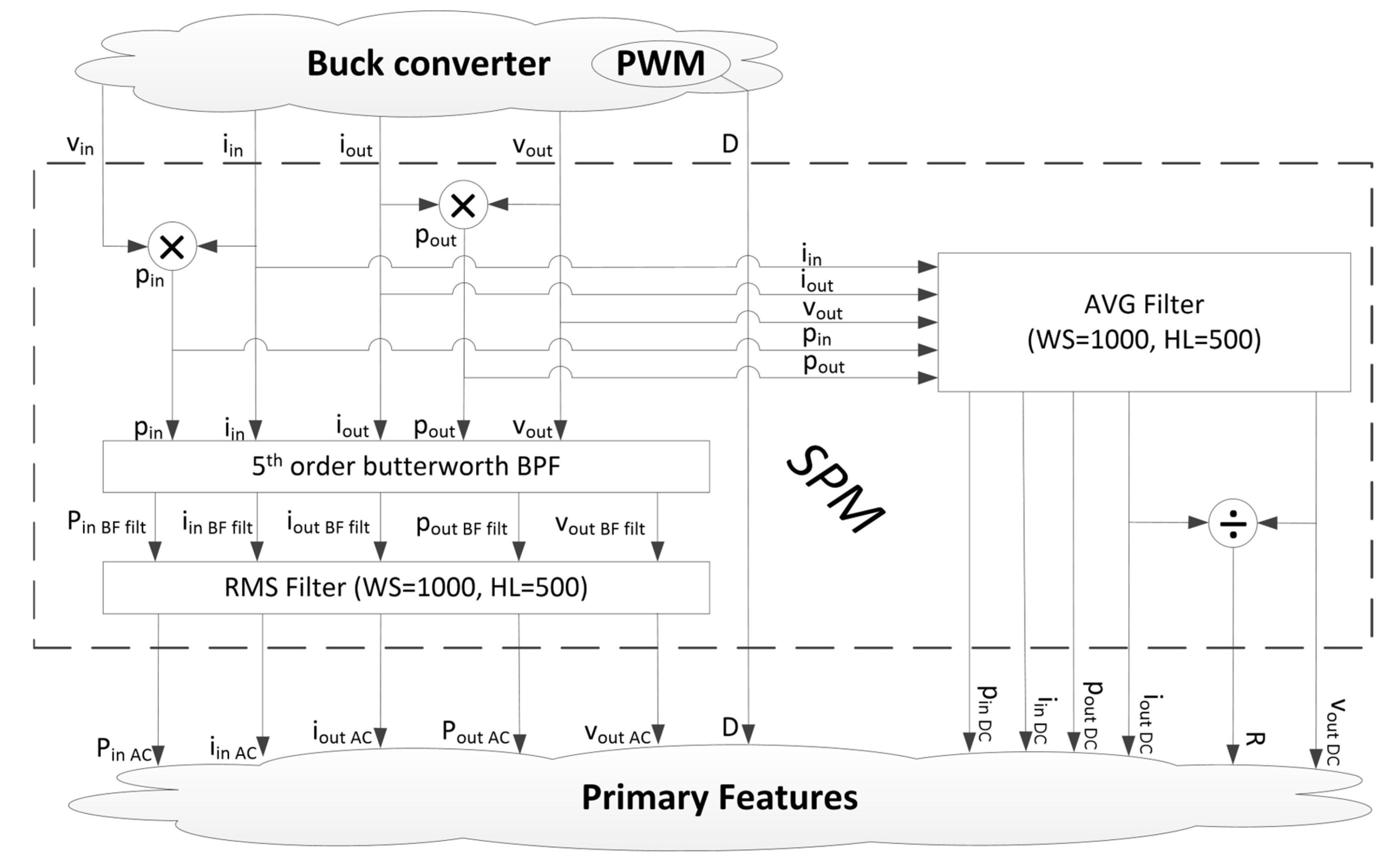
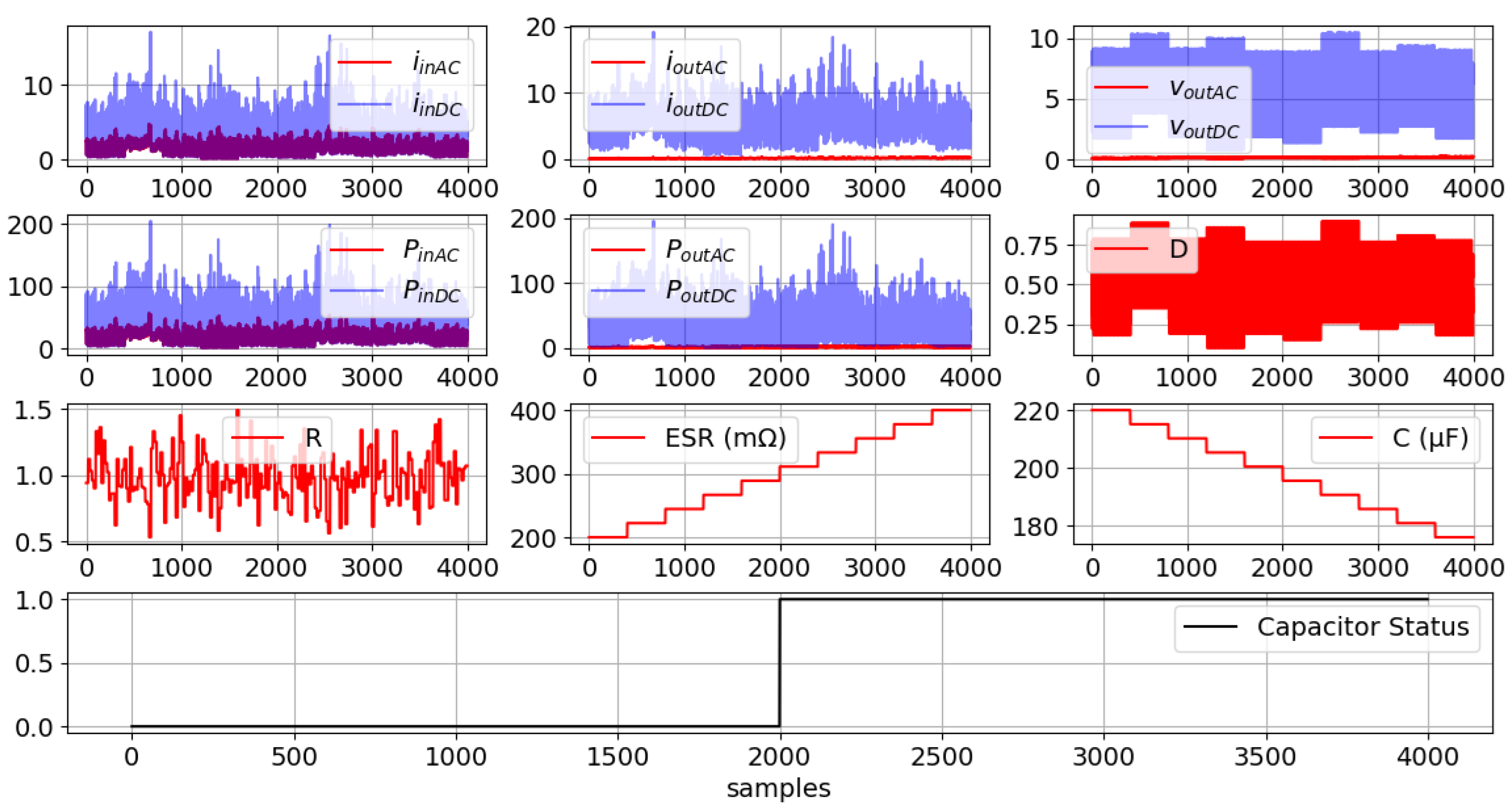
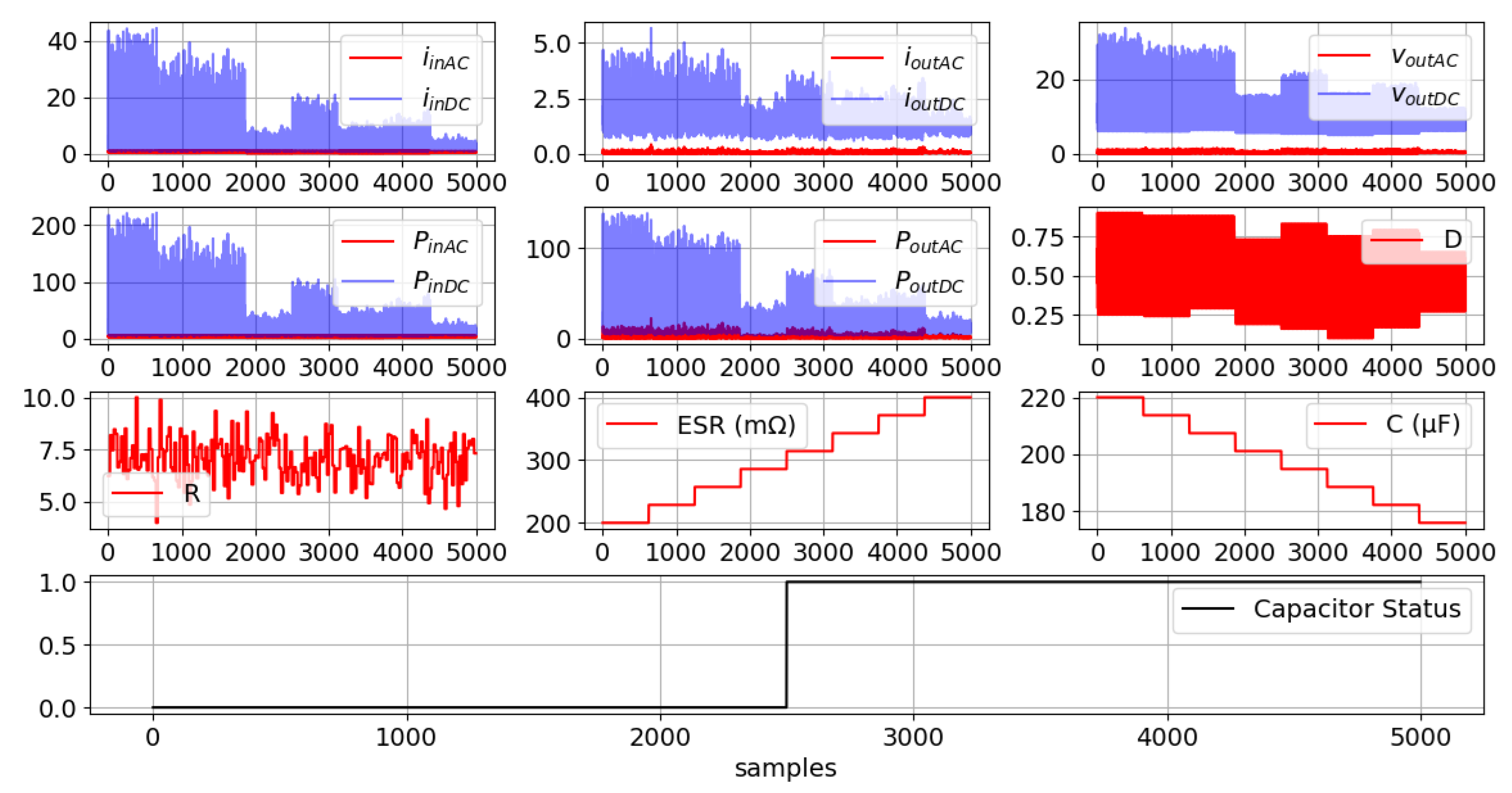
4.2. Signal Processing Module (SPM)

The signal processing module (SPM) is responsible for extracting the primary features of the raw data (Figure 4).

The primary features correspond to the DC and AC components of the raw signals. The DC components are extracted using a moving average filter (AVG Filter) with a window size (WS) of 1000 samples and a hope size (HS) of 500 samples. The AC components are extracted in two stages: first, the raw signals pass through a fifth-order bandpass filter (BDF) that isolates the signal component around the converter’s switching frequency (20 kHz); then, an RMS filter with a WS of 1000 samples and a HS of 500 samples is applied to compute the AC features.

Figure 4 shows that two new raw variables, the input power (p_in) and output power (p_out), were generated through a simple multiplication of the original raw variables (v_in, i_in, v_out, and i_out).

Through the aforementioned transformations, 10 primary features were generated. In addition, a new feature (R) was created using two of these primary features, and the duty cycle was included, which requires no additional sensors as it is provided by the PWM. This resulted in a total of 12 primary features, which are summarized below:

• P_inAC—represents the AC component of p_in;
• P_inDC—represents the DC component of p_in;
• P_outAC—represents the AC component of p_out;
• P_outDC—represents the DC component of p_out;
• i_inAC—represents the AC component of i_in;
• i_inDC—represents the DC component of i_in;
• i_outAC—represents the AC component of i_out;
• i_outDC—represents the DC component of i_out;
• v_outAC—represents the AC component of v_out;
• v_outDC—represents the DC component of v_out;
• R—represents the load resistance, calculated as v_outDC divided by i_outDC;
• D—represents the duty cycle provided by the PWM.

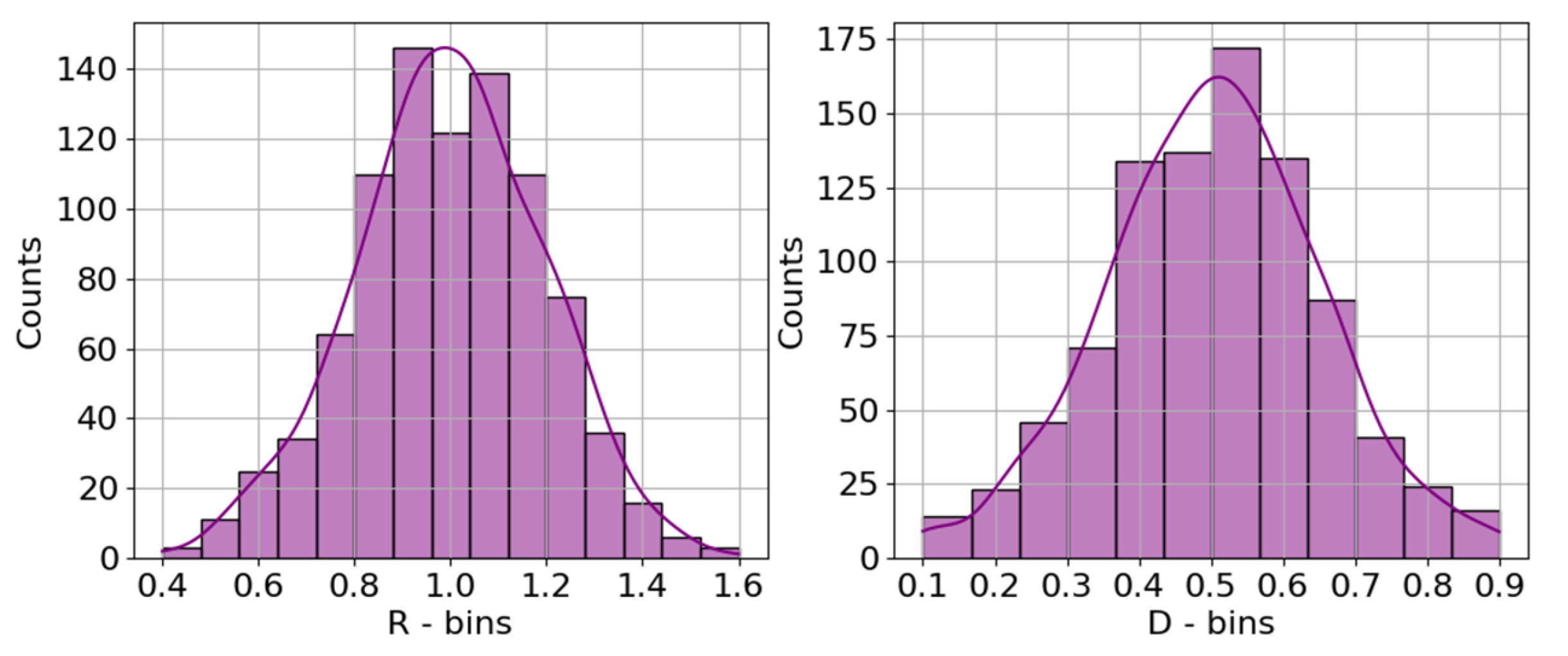
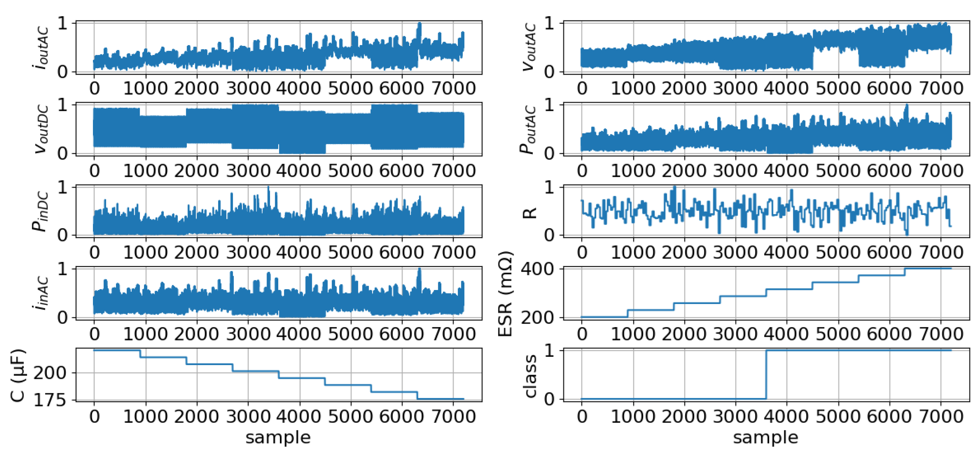
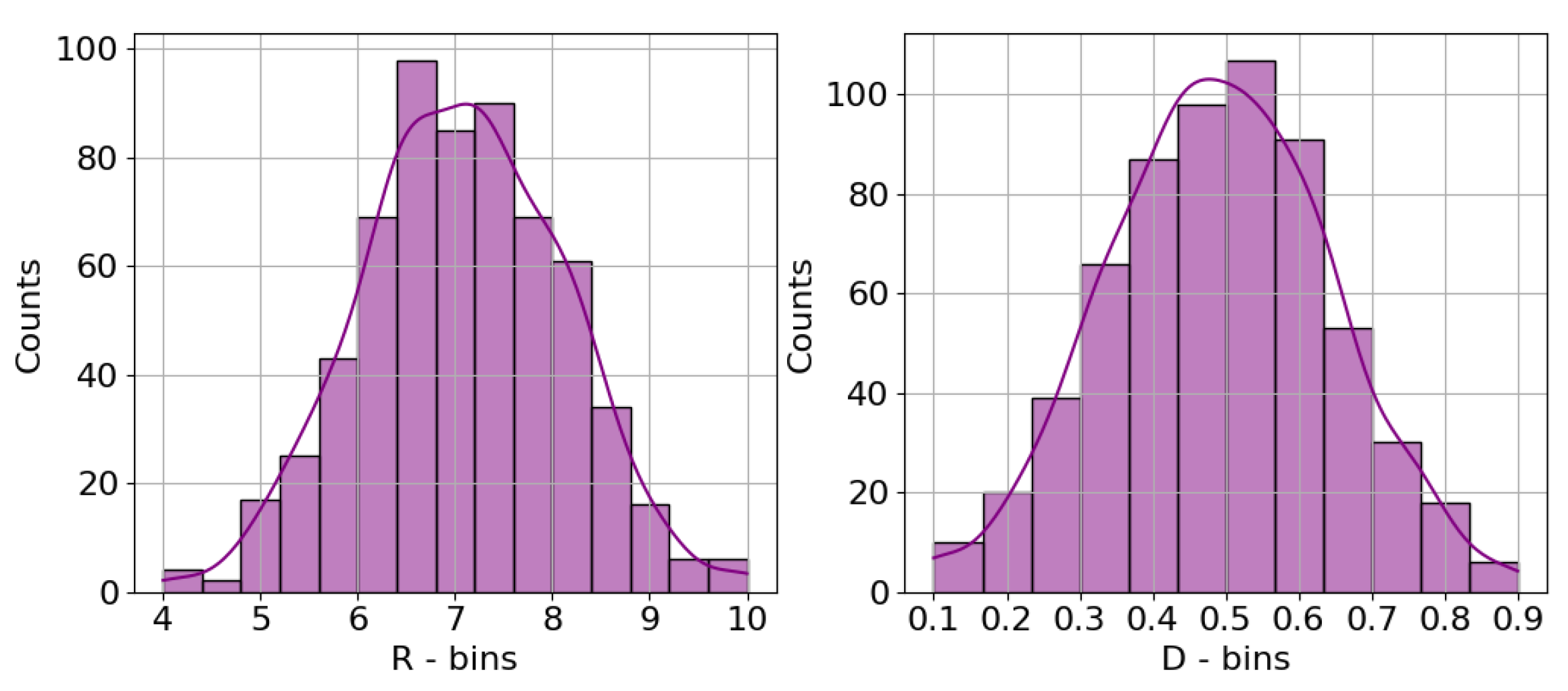
4.3. Dataset Generation Workflow

The complete process of raw data generation and subsequent processing used to construct the original dataset is detailed below. Initially, the buck converter was simulated across a wide range of operating conditions using the method proposed in [59]. This approach allows the simulation of buck converters in Python (version 3.13.2) and has been validated using the LTspice simulation software (version (x64): 24.0.12), the latter being considered the gold standard. LTspice is a powerful simulation software and is commonly used in academia and industry due to its accuracy in simulating electrical circuits [60]. Both simulation tools produced equivalent results, as demonstrated in [21,59].

The simulation tool proposed in [59] enables the efficient and automated execution of numerous simulations across various scenarios using a simplified and scalable process. This method enables the creation of a dataset with different operating conditions, supporting the training of ML algorithms for integration into FDTs.

Initially, to ensure that the simulated behavior closely mirrors that of a commercial buck converter, a set of 900 different operating conditions was randomly defined. In this way, the values of the duty cycle (D) and the load resistance (R) were generated to approximate a normal distribution. Regarding the R, an average of 1 Ω with a standard deviation of 0.3 was used, and the values were restricted to the range of 0.4–1.6 Ω (Figure 5). For the D, an average of 0.5 and a standard deviation of 0.15 were used, with a range of values between 0.1 and 0.9 being considered (Figure 5). The histograms of both distributions, shown in Figure 5, closely resemble a normal distribution.

In addition, eight different scenarios, corresponding to eight levels of failure severity (S₀, S₁, S₂, S₃, S₄, S₅, S₆, and S₇) of the al-cap, were created for each of the 900 operating conditions, as shown in Figure 6. Hence, the total number of simulations required to create the initial dataset was 8 × 900, which corresponds to a total of 7200 distinct simulations.

Figure 7 presents the complete dataset used to train and test the machine learning models, comprising 7200 distinct simulations. For each simulation, a sample was extracted which contained the 12 primary features, as well as the target, the capacitor status (0—normal state and 1—faulty state).

Figure 7 further illustrates the ESR and C values, from which it can be inferred that the failure threshold defined in this study corresponds to an ESR increase to 1.5 times that of a sound capacitor, which corresponds to 300 mΩ, and a capacitance degradation of 10% relative to its nominal value, which corresponds to 198 μF.

5. Information Processing Module (IPM) Design

This paper presents the design of a FDT that combines a SPM with a ML algorithm to assess the condition of capacitors in power electronic systems. Therefore, it constitutes an ML-driven project that follows a structured sequence of stages, beginning with problem definition and data collection, both of which were discussed in earlier sections. The subsequent phases include exploratory data analysis (EDA), model training and evaluation, and, ultimately, model implementation or deployment.

Hence, the information processing module (IPM) should incorporate all of these steps, with the exception of the deployment stage, which will be covered in Section 6.

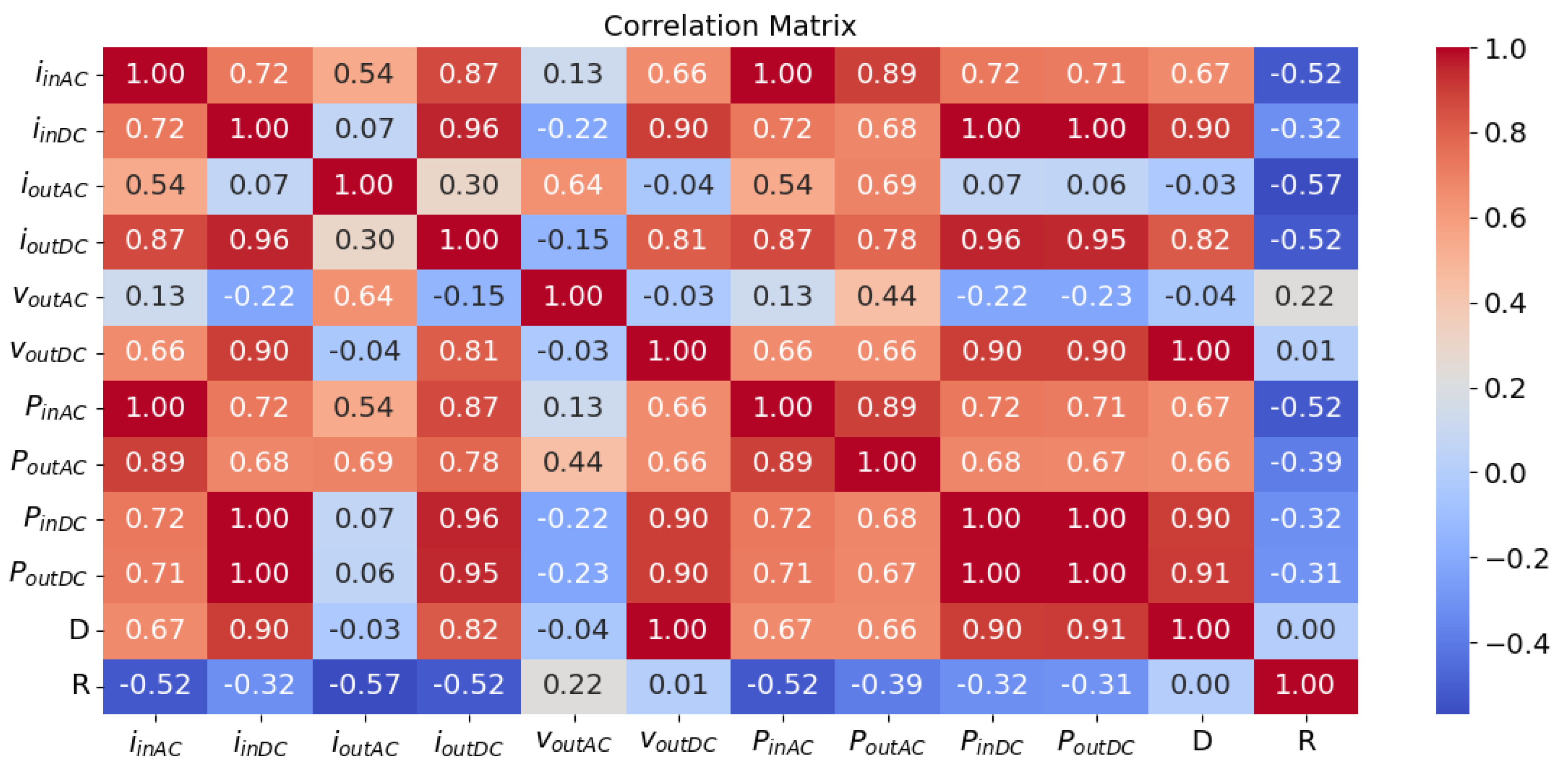
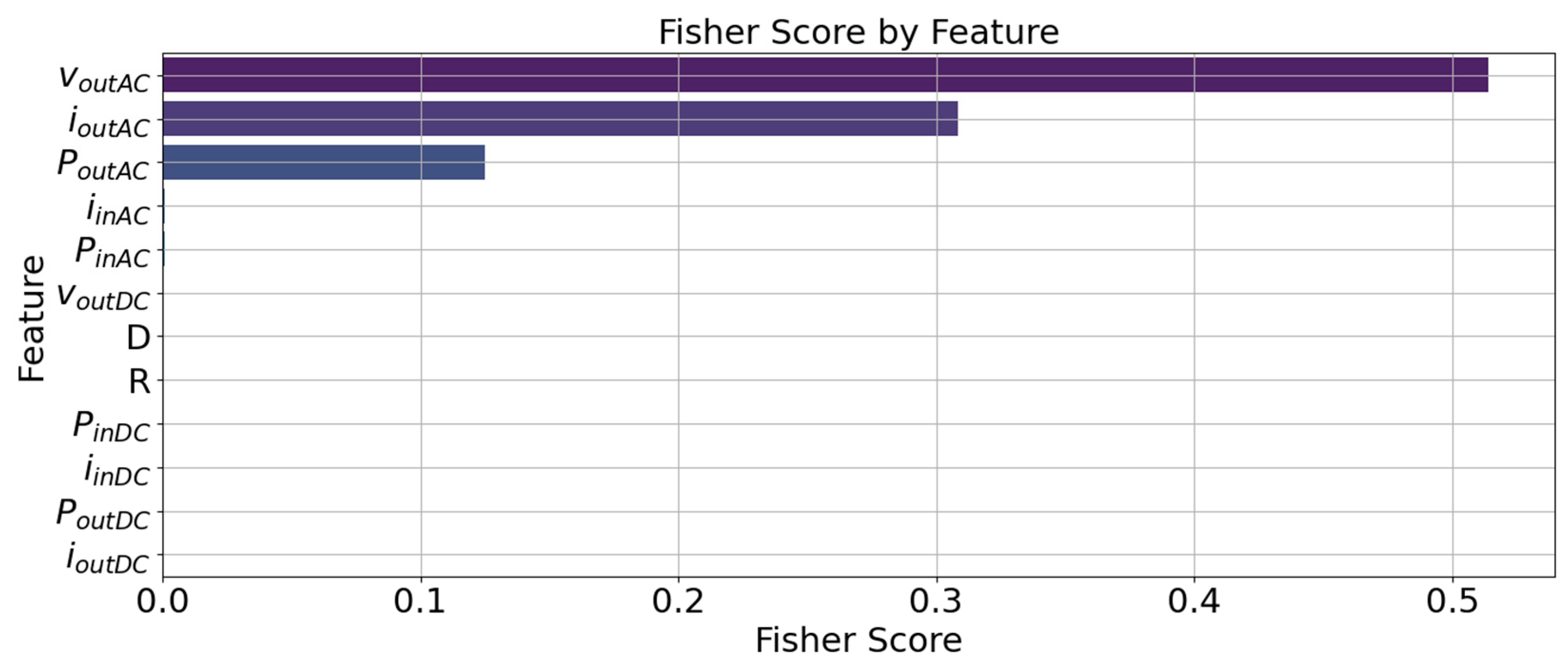
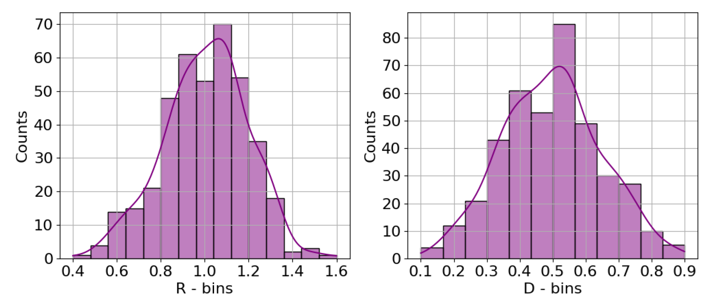
5.1. Exploratory Data Analysis (EDA)

The exploratory data analysis (EDA) process begins with gaining a clear understanding of the original dataset, including recognizing its features and target variables. The original dataset contains 12 numerical features (P_inAC, P_inDC, P_outAC, P_outDC, i_inAC, i_inDC, i_outAC, i_outDC, v_outAC, v_outDC, R, and D) and one categorical target (capacitor status).

Next, it is important to consider whether any additional processing is needed, such as dealing with duplicate entries or missing values. In the original dataset, no missing values or duplicate records were found. However, Figure 7 suggests the presence of outliers in some features, which is why individual boxplots (Figure 8) were created for each of the features to better visualize their distributions.

The preceding figure clearly highlights the presence of outliers in the features related to current and power. However, these outliers will not be removed, as the goal is for the proposed solution to assess the capacitor’s condition even under extreme operating conditions.

The performance of ML models is highly influenced by the features used for prediction. Therefore, selecting the most relevant features is crucial to optimizing the model’s performance. Irrelevant features can increase the model’s complexity, increase the computation time, and often lead to overfitting [51,61]. Identifying and removing irrelevant features from the dataset is an essential step before starting the ML model training stage.

The reduction of features is based on their relevance and redundancy in relation to the target. Thus, features can be classified as strongly relevant, weakly relevant but not redundant, irrelevant, or redundant [61]. Relevant features should be retained unless they are highly correlated with other equally relevant features. Although weakly relevant features may not contribute significantly to ML model learning, they will be preserved in this case as long as they are not strongly correlated with each other, for two main reasons: first, the total number of features is relatively small; the second is due to the fact that some weakly relevant features allow the model to identify the operating state of the converter, which is essential to avoiding incorrect classification of the capacitor condition, particularly under extreme operating conditions. In this context, it is important to highlight that PCs are intrinsically non-linear systems, which adds significant complexity and other challenges to the learning process of ML models. Consequently, it is crucial that the ML model reliably identifies the converter’s operational state to ensure accurate performance. Irrelevant features, particularly those that do not help the ML model to identify the converter’s operating condition or the capacitor’s condition, as well as redundant features, will be removed from the final dataset.

To evaluate the redundancy among two features, X and Y, the Pearson correlation coefficient was computed as follows [51]:

$$r={\displaystyle \frac{n\times \sum \left(X\times Y\right)-\sum X\times \sum Y}{\sqrt{\left(n\times \sum X^2-{\left(\sum X\right)}^2\right)\times \left(n\times \sum Y^2-{\left(\sum Y\right)}^2\right)}}}$$

(1)

where n represents the number of samples (7200).

Figure 9 illustrates the correlations among all features.

For this problem, a maximum correlation threshold of 0.95 was established to identify pairs of redundant features [62,63]. Therefore, based on the analysis of the preceding figure, the following features have been identified as redundant:

• The features i_inAC and P_inAC have been identified as redundant due to their high correlation (r ≥ 0.95);
• The features i_inDC, i_outDC, P_inDC, and P_outDC have been identified as redundant due to their high correlation (r ≥ 0.95);
• The features v_outDC and D have been identified as redundant due to their high correlation (r ≥ 0.95);

Once the redundant features have been identified, it is crucial to remove those that are less relevant and redundant. To achieve this, two feature selection methods will be employed. Feature selection methods are commonly classified into the following: filters, wrappers, and embedded and hybrid methods [61]. In this study, two filter-based methods will be applied, as they enable feature selection independently of the ML model. Filter-type methods can be categorized into two types: univariate and multivariate approaches. The former evaluates each feature individually, allowing the creation of a ranking of the most important features (Figure 10 and Figure 11), while multivariate approaches evaluate subsets of features collectively. This article employs two univariate techniques commonly used in classification tasks: mutual information gain and the Fisher score [61].

Mutual information (MI) is a statistical metric used to quantify the dependency between two variables (X and Y), capturing both linear and non-linear relationships. It can be computed as follows [64,65]:

$$MI\left(X;Y\right)={\sum }_{x,\mathrm{y}}p\left(x,y\right) log\left({\displaystyle \frac{p\left(x,y\right)}{p\left(x\right)p\left(y\right)}}\right)$$

(2)

where the joint probability distribution of X and Y is represented by $p\left(x,y\right)$, while $p\left(x\right)$ and $p\left(y\right)$ indicate the marginal probability distribution of X and Y, respectively.

In this case, the goal is to assess the strength of dependence between each feature (X) and the target (Y). Figure 10 presents the features ranked by their relevance, which is based on the mutual information (MI) values.

Figure 10 reveals that v_outAC, i_outAC, and P_outAC demonstrate the highest mutual information values with respect to the target variable (capacitor status or class), whereas D and i_outDC exhibit the lowest values. Although certain features show reduced MI values, this reduction is not substantially pronounced.

Therefore, the Fisher score (FS) was employed for further analysis, and the features were ranked by their relevance (Figure 11).

The FS of feature $f^j$ can be computed as follows [64,65]:

$$FS\left(f^j\right)={\displaystyle \frac{{\sum }_{l=1}^c{n}_l{\left({\mu }_l^j-{\mu }^j\right)}^2}{{\sum }_{l=1}^c{n}_l{\left({\sigma }_l^j\right)}^2}}$$

(3)

where ${\mu }_l^j$ and ${\sigma }_l^j$ represent the mean and standard deviation of the l class corresponding to feature $f^j$, ${\mu }^j$ denotes the mean of $f^j$, c represents the number of classes, and $n_l$ the number of samples for label l.

Since the features i_outAC, v_outAC, P_outAC, and R exhibit correlation values below the predetermined threshold (r < 0.95) with all other features, they are retained for three primary reasons. Firstly, aging induces an increase in the capacitor impedance, which consequently affects the output current, voltage, and power; secondly, v_outAC, i_outAC, and P_outAC demonstrate the highest mutual information (MI) values and Fisher scores (FS) relative to the target variable. Third, the R feature plays a crucial role in accurately determining the power converter operational status.

Subsequently, the remaining features were selected based on inter-feature correlations, as well as their MI and FS with the target variable:

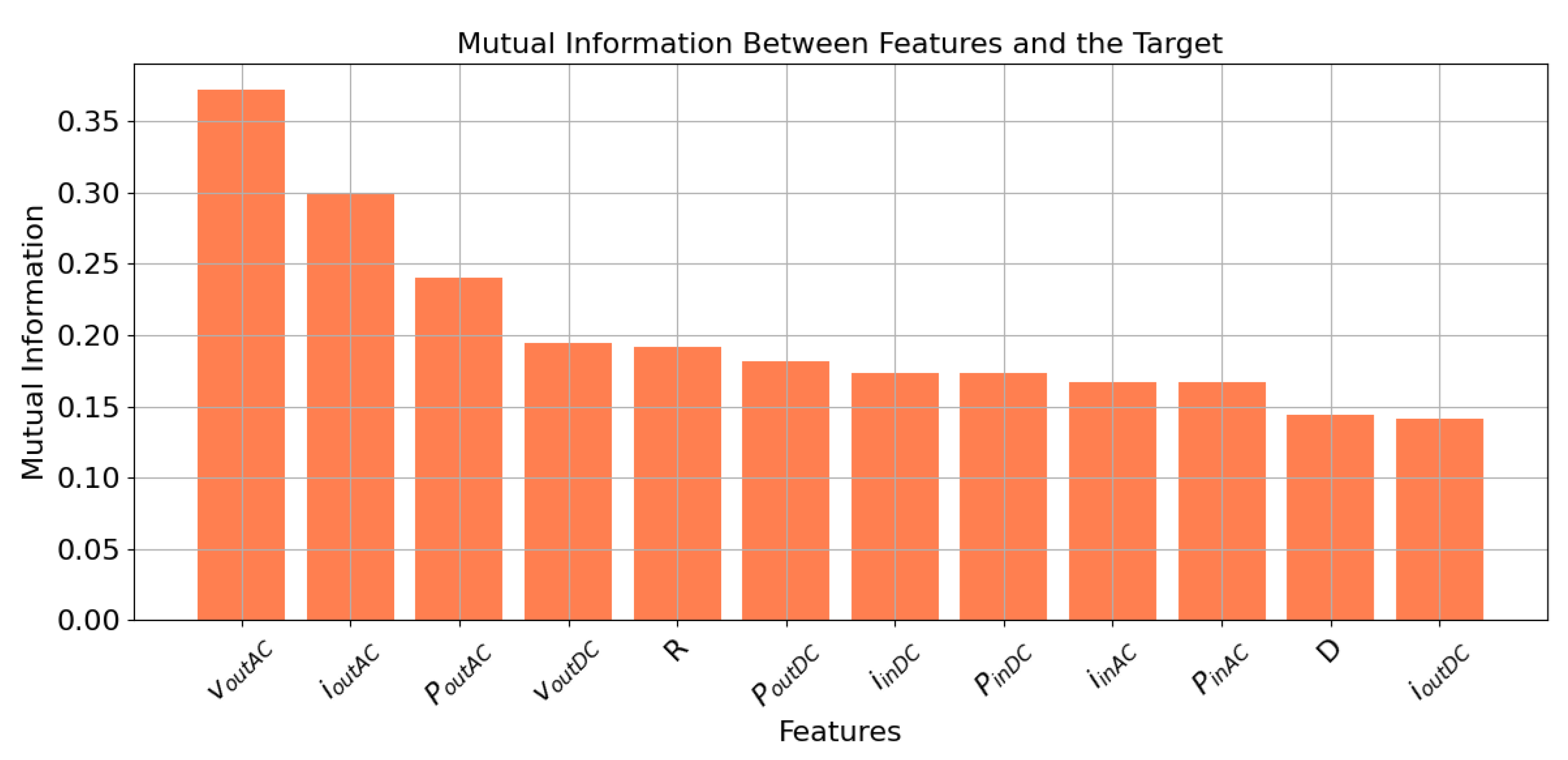
• From the feature set {i_inDC, i_outDC, P_inDC, and P_outDC}, only P_inDC was retained due to having the highest FS value;
• From the feature set {P_inAC, i_inAC}, i_inAC was retained based on its superior MI and FS values;
• From the feature set {v_outDC, DC}, v_outDC was chosen due to having the highest MI and FS values.

To summarize, the final input features of the ML model include the following:

• i_outAC—represents the AC component of i_out;
• v_outAC—represents the AC component of v_out;
• P_outAC—represents the AC component of p_out;
• R—represents the load resistance;
• P_inDC—represents the DC component of p_in;
• i_inAC—represents the AC component of i_in;
• v_outDC—represents the DC component of v_out.

Figure 12 presents the final dataset after feature normalization to ensure that all features contribute equally to the model. A min-max scaling transformation was applied to achieve feature normalization (4):

$$X_{normalized}={\displaystyle \frac{X-X_{min}}{X_{max}-X_{min}}}$$

(4)

where X represents the actual feature value, X_min the minimum value of X in the dataset, and X_max the maximum value of X in the dataset.

5.2. Logistic Regression (LR)

Unlike linear regression (LinR), which predicts values from a continuous and infinite range, classification models predict outcomes from a limited set of discrete classes, which makes them a more appropriate solution for the problem under analysis.

In the current problem, the number of classes is clearly two, as the target variable can take just two possible values: “No Fault” and “Fault” (Figure 3). In this context, the positive class (class 1) represents the “Fault” condition, while the negative class (class 0) corresponds to the “No Fault” condition.

Logistic regression (LR) is a ML classification model that estimates the probability of a class occurring for a given combination of feature values. To do so, it applies the logistic (sigmoid) function to a linear combination of the input features, where the importance of each feature is determined by its corresponding coefficient.

In LinR, the target, $t_{lin}$, presents a linear relationship with a set of features, $f=\left(f_1,\dots ,f_N\right)$, as can be seen in Equation (5):

$${\widehat{t}}_{lin}\left(f_1,\dots ,f_N\right)=k_0+k_1·f_1+{\dots +k}_N·f_N$$

(5)

where ${\widehat{t}}_{lin}$ represents the predicted target and $\left(k_0,\dots ,k_N\right)$ represent the model coefficients.

Therefore, by combining (5) with the sigmoid function (σ(t)), it is possible to derive the fundamental model for the LR.

$$LR\left(f\right)=\sigma \left(t_{lin}\left(f_1,\dots ,f_N\right)\right)={\displaystyle \frac{1}{1+e^{-\left({\mathrm{t}}_{lin}\left(f_1,\dots ,f_N\right)\right)}}}={\displaystyle \frac{1}{1+e^{-\left(k_0+k_1·f_1+{\dots +k}_N·f_N\right)}}}$$

(6)

Equation (6) defines a parametric model that is characterized by the coefficients $\left(k_0,\dots ,k_N\right)$ and which estimates the probability that a sample of dataset DS, defined by a specific combination of feature values, is associated with class 1:

$$\begin{gathered} given:DS=\left\{\begin{array}{c}features:f=\left(f_1,\dots ,f_N\right)\\ target:t=\left(‘class0’,‘class1’\right)\end{array}\Rightarrow {\widehat{t}}_{log}\approx t;{\widehat{t}}_{log}=\left\{\begin{array}{c}‘class 0’, if LR\left(f\right)<0.5\\ ‘class 1’, if LR\left(f\right)\ge 0.5\end{array}\right.\right. \\ as:LR\left(f\right)=0.5\iff t_{lin}\left(f_1,f_2,\dots ,f_N\right)=0\Rightarrow {\widehat{t}}_{log}=\left\{\begin{array}{c}‘class 0’, if {\mathrm{t}}_{lin}\left(f_1,f_2,\dots ,f_N\right)<0\\ ‘class 1’, if {\mathrm{t}}_{lin}\left(f_1,f_2,\dots ,f_N\right)\ge 0\end{array}\right. \end{gathered}$$

(7)

where $LR\left(f\right)$ represents the probability of class 1 occurring, ${\widehat{t}}_{log}$ represents the class prediction, $t_{lin}\left(f_1, f_2,\dots ,f_N\right)$ the decision boundary (DB), and $t$ the real class.

Decision boundaries (DBs) can be either linear (LDBs) or non-linear (NLDBs). While NLDBs can model complex relationships that linear boundaries cannot capture, they also substantially increase the model complexity, computational cost, and risk of overfitting. For this reason, the proposed LR model, $PLR\left(f\right)$, is based on a linear decision boundary (LDB), as shown in Equation (8).

$$PLR\left(f\right)={\displaystyle \frac{1}{1+e^{-\left(k_0·i_{\mathrm{o}\mathrm{u}\mathrm{t}\mathrm{A}\mathrm{C}}+k_1·v_{\mathrm{o}\mathrm{u}\mathrm{t}\mathrm{A}\mathrm{C}}+k_2·v_{\mathrm{o}\mathrm{u}\mathrm{t}\mathrm{D}\mathrm{C}}+k_3·P_{\mathrm{o}\mathrm{u}\mathrm{t}\mathrm{A}\mathrm{C}}+k_4·P_{\mathrm{i}\mathrm{n}\mathrm{D}\mathrm{C}}+k_5·\mathrm{R}+k_6·i_{\mathrm{i}\mathrm{n}\mathrm{A}\mathrm{C}}+k_7\right)}}}$$

(8)

Thus, once the model has been identified, it is necessary to determine the coefficients $\left(k_0,\dots ,k_7\right)$ that best fit the classification problem. This procedure is performed during the training stage, the main objective of which is to find the model coefficients that maximize the likelihood of ${\widehat{t}}_{log}=t$ for each sample in the training dataset.

Hence, it is essential to identify a cost function that enables the evaluation of how effectively the $\left(k_0,\dots ,k_7\right)$ parameters allow the $PLR\left(f\right)$ model to better fit the training dataset. Given the nature of the logistic function, the cost function commonly used in LinR, ${CF}_{linR}$, is not suitable for LR, as it would generate a non-convex function that would have multiple local minima.

$${CF}_{linR}\left(k_0,k_1,\dots ,k_N\right)={\displaystyle \frac{1}{m}}{\sum }_{i=1}^m{\left({\widehat{t}}_{lin}\left[i\right]-t_{lin}\left[i\right]\right)}^2$$

(9)

In order to address the previous mentioned issue, the loss function, LF, presented below is typically used:

$$LF\left(PLR\left(f\left[i\right]\right),t\left[i\right]\right)=\left\{\begin{array}{c}-log\left(PLR\left(f\left[i\right]\right)\right), if t\left[i\right]=1\\ -log\left(1-PLR\left(f\left[i\right]\right)\right), if t\left[i\right]=0\end{array}\right.$$

(10)

Assuming that sample i corresponds to a positive class ($t\left[i\right]=1$), if the estimated probability is close to 1 ($PLR\left(f\left[i\right]\right)$≈ 1), then the value of the LF will be $-log\left(1\right)=0$, which indicates not penalizing the chosen parameters. If, on the contrary, the estimated probability is close to zero ($PLR\left(f\left[i\right]\right)$≈ 0), the LF will be $-log\left(0\right)=+\infty$, which indicates significantly penalizing the choice of parameters and forcing an optimization of the parameters. A similar reasoning applies when the target belongs to the negative class; therefore, assuming that sample i corresponds to $t\left[i\right]=0$, if $PLR\left(f\left[i\right]\right)$≈ 0, then the value of the LF will be $-log\left(1-0\right)=0$, which indicates not penalizing the chosen parameters. If, on the contrary, $PLR\left(f\left[i\right]\right)$≈ 1, the LF will be $-log\left(1-1\right)=+\infty$, which indicates significantly penalizing the choice of parameters and forcing an optimization of the parameters.

Finally, it is possible to write the cost function for the m samples of the training dataset, ${CF}_{LR}$, as follows:

$${CF}_{LR}\left(k_0,\dots ,k_N\right)={\displaystyle \frac{1}{m}}{\sum }_{i=1}^{m}LF\left(PLR\left(f\left[i\right]\right),t\left[i\right]\right)$$

(11)

In turn, (11) can be rewritten in a single simplified equation:

$${CF}_{LR}\left(k_0,\dots ,k_N\right)=-{\displaystyle \frac{1}{m}}{\sum }_{i=1}^m\left(\log \left(PLR\left(f\left[i\right]\right)\right)\times t\left[i\right]+log\left(1-PLR\left(f\left[i\right]\right)\right)\times \left(1-t\left[i\right]\right)\right)$$

(12)

The subsequent step involves finding the minimum of (12) by applying an optimization solver like the gradient descent algorithm to ensure optimal values for $\left(k_0,\dots ,k_7\right)$.

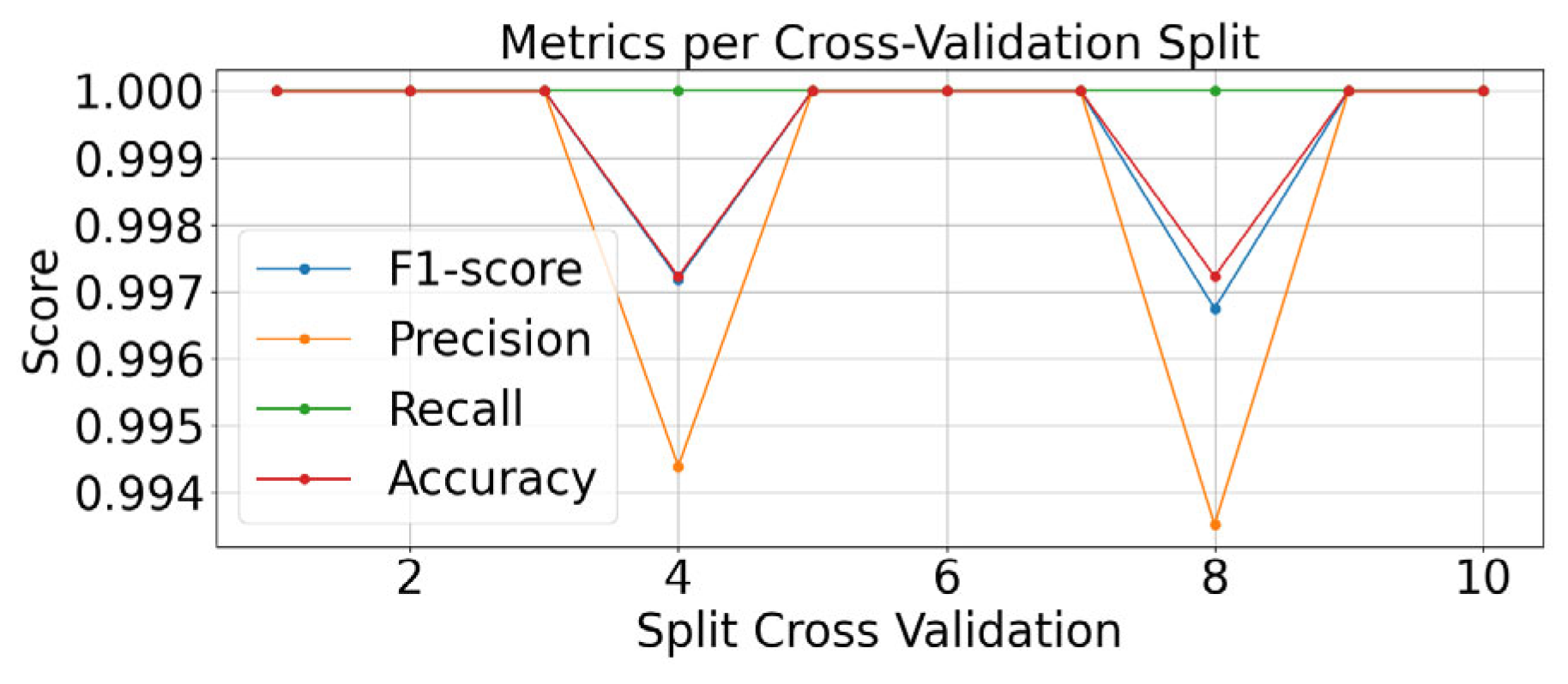
5.3. Cross Validation

This section aims to demonstrate that the chosen LDB, although simple, is well suited to the problem, and thereby eliminates the need for additional feature engineering. Therefore, it is essential to assess not only the model’s performance but also its ability to generalize, which justifies the use of cross-validation.

Therefore, from the final dataset (Figure 12), 50% of the samples were randomly selected to create a new dataset, the training dataset (TrainDS), as shown in Figure 13.

Sequentially, the TrainDS was divided into 10 equally sized folds. The model was trained and evaluated 10 times with a different fold being used for testing each time and the remaining nine for training. This approach ensures that every sample is used once for testing and nine times for training. Four commonly used metrics for classification problems were employed to evaluate the model’s performance: accuracy, precision, recall, and F1 score.

To gain a clearer understanding of the concepts of accuracy, precision, recall, and F1 score, it is essential to first define the following terms:

• True positive (TP)—represents the number of correct predictions that identify the ”Fault” condition;
• False positive (FP)—represents the number of incorrect predictions that identify the ”Fault” condition;
• True negative (TN)—represents the number of correct predictions that identify the ”No Fault” condition;
• False negative (FN)—represents the number of incorrect predictions that identify the ”No Fault” condition.

In the cases of a TP or FP, the ML model returns a ‘1’, and in the case of a TN or FN, the model will return a ‘0’.

Thus, it is possible to define accuracy as follows:

$$Accuracy={\displaystyle \frac{TP+TN}{TP+FP+TN+FN}}$$

(13)

Accuracy is a suitable metric for balanced datasets, those in which the number of positive and negative samples is approximately equal. In the case of TrainDS, the dataset contains 1828 negative-class samples and 1772 positive-class samples, which reflects a balanced distribution.

Precision represents how accurate the model is when it predicts a ‘1’, and can be represented by the following equation:

$$Precision={\displaystyle \frac{TP}{TP+FP}}$$

(14)

Recall represents how accurate the model is when the true class is predicted as a ‘1’, and can be represented by the following equation:

$$recall={\displaystyle \frac{TP}{TP+FN}}$$

(15)

Finally, we present the F1 score, a metric that represents a trade-off between precision and recall, and for this purpose calculates its harmonic mean. The F1 score offers a single metric that highlights cases where either the precision or recall is significantly low.

$$F1 score=2\times {\displaystyle \frac{Precision\times Recall}{Precision+Recall}}$$

(16)

Figure 14 presents the various metrics across each cross-validation split.

Figure 14 clearly indicates that the model does not exhibit overfitting on the training dataset and demonstrates strong overall performance.

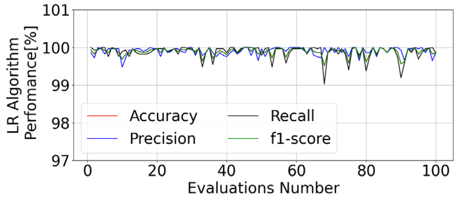
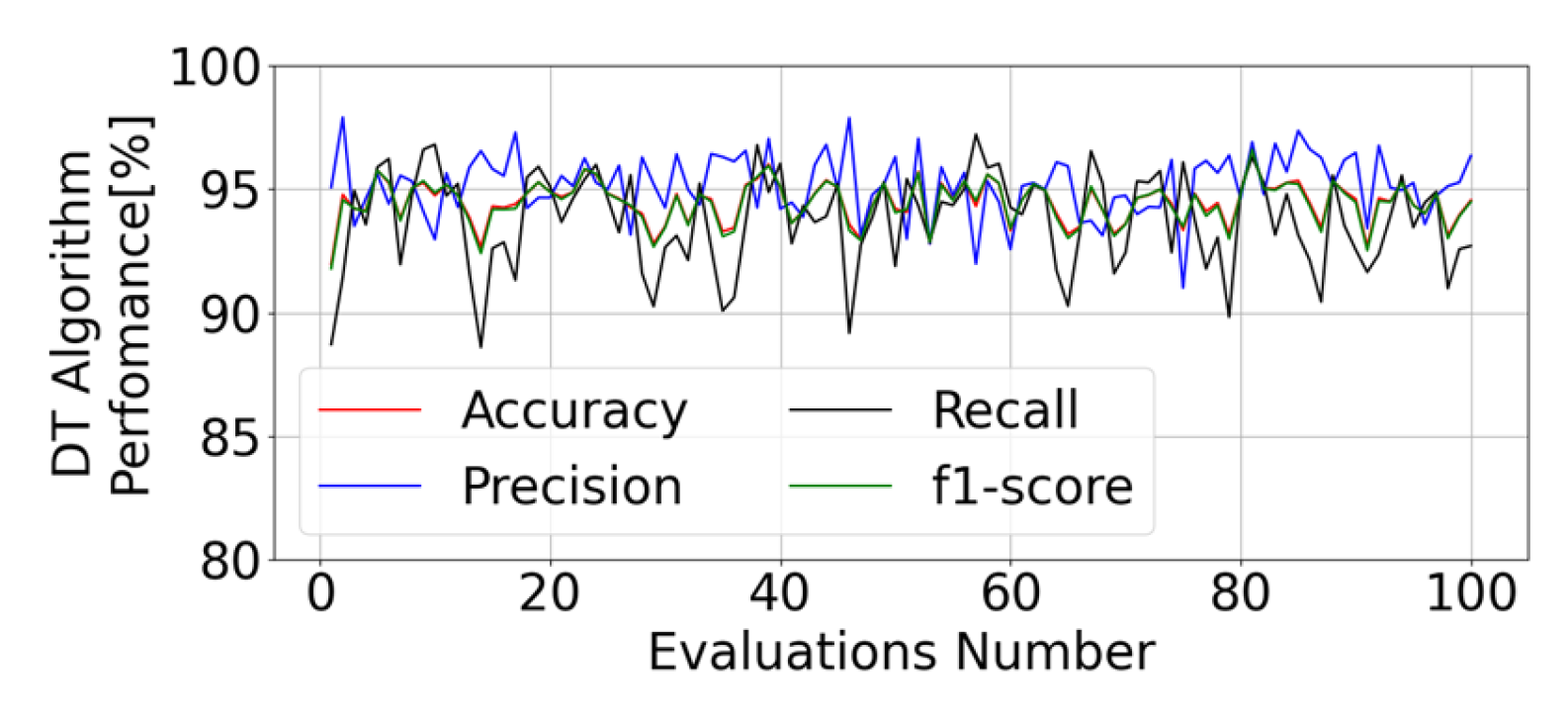
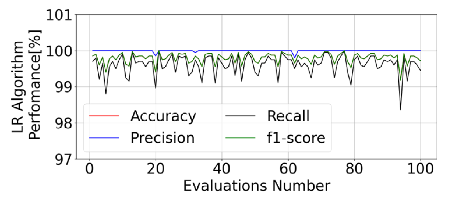
5.4. Model Training and Evaluation

In order to strengthen the conclusions from the previous section, the model was trained and tested on the full dataset (Figure 12) through 100 independent evaluations. In each evaluation, 20% of the original samples were randomly selected for training, while the remaining 80%, unseen by the model, were used for testing. The training and testing sets were unique in each run. The performance outcomes of the 100 trained and tested models are illustrated in Figure 15.

The 100 models demonstrated consistently high performance, with the mean accuracy, precision, recall, and F1 scores all exceeding 99.8%.

Considering that the FDT prioritizes simplified implementation on microcontrollers, two ML algorithms are particularly well suited for this binary classification task: logistic regression and decision trees. The LR model only requires the evaluation of whether the decision boundary is greater than zero, which eliminates the need to calculate the sigmoid and makes the model computationally efficient. Decision trees offer variable complexity, which depends on the depth of the tree: shallow trees require fewer sequential comparisons and corresponding “if-else” statements, while deeper trees demand more.

A decision tree-based FDT was implemented to compare its performance against the LR FDT solution. The decision tree (DT) model was implemented with specific constraints to facilitate its implementation on a microcontroller and improve its generalization. The DT model was limited to a maximum depth of 6 and a minimum of 10 samples required to split an internal node, as both constraints improve the generalization of the model and maintain the simplicity of its implementation. The DT model demonstrated lower performance compared to LR. Following the same evaluation protocol applied to LR, the DT model was trained and tested on the full dataset (Figure 12) through 100 independent runs (Figure 16).

Analysis of these 100 DT models revealed an average performance below 95.1% across all metrics.

Therefore, the LR model from the final evaluation (n° = 100) shown in Figure 15 was selected for FDT implementation. The LR model parameters are detailed below.

$$\begin{array}{l}PLR\left(i_{\mathrm{o}\mathrm{u}\mathrm{t}\mathrm{A}\mathrm{C}},v_{\mathrm{o}\mathrm{u}\mathrm{t}\mathrm{A}\mathrm{C}},v_{\mathrm{o}\mathrm{u}\mathrm{t}\mathrm{D}\mathrm{C}},P_{\mathrm{o}\mathrm{u}\mathrm{t}\mathrm{A}\mathrm{C}},P_{\mathrm{i}\mathrm{n}\mathrm{D}\mathrm{C}},R,i_{\mathrm{i}\mathrm{n}\mathrm{A}\mathrm{C}}\right)\\ \hspace{1em}\hspace{1em}\hspace{1em}\hspace{1em}={\displaystyle \frac{1}{1+e^{-\left(k_0·i_{\mathrm{o}\mathrm{u}\mathrm{t}\mathrm{A}\mathrm{C}}+k_1·v_{\mathrm{o}\mathrm{u}\mathrm{t}\mathrm{A}\mathrm{C}}+k_2·v_{\mathrm{o}\mathrm{u}\mathrm{t}\mathrm{D}\mathrm{C}}+k_3·P_{\mathrm{o}\mathrm{u}\mathrm{t}\mathrm{A}\mathrm{C}}+k_4·P_{\mathrm{i}\mathrm{n}\mathrm{D}\mathrm{C}}+k_5·\mathrm{R}+k_6·i_{\mathrm{i}\mathrm{n}\mathrm{A}\mathrm{C}}+k_7\right)}}}\\ \left(k_0,k_1,k_2,k_3,k_4,k_5,k_6,k_7\right)\approx \left(113.5,-55.2,-124.6,863.9,174.3,27.3,-833.9,-11.7\right)\\ {FDT}_{Pre}=\left\{\begin{array}{c}‘class 0’, if PLR\left(i_{\mathrm{o}\mathrm{u}\mathrm{t}\mathrm{A}\mathrm{C}},v_{\mathrm{o}\mathrm{u}\mathrm{t}\mathrm{A}\mathrm{C}},v_{\mathrm{o}\mathrm{u}\mathrm{t}\mathrm{D}\mathrm{C}},P_{\mathrm{o}\mathrm{u}\mathrm{t}\mathrm{A}\mathrm{C}},P_{\mathrm{i}\mathrm{n}\mathrm{D}\mathrm{C}},R,i_{\mathrm{i}\mathrm{n}\mathrm{A}\mathrm{C}}\right)<0.5\\ ‘class 1’, if PLR\left(i_{\mathrm{o}\mathrm{u}\mathrm{t}\mathrm{A}\mathrm{C}},v_{\mathrm{o}\mathrm{u}\mathrm{t}\mathrm{A}\mathrm{C}},v_{\mathrm{o}\mathrm{u}\mathrm{t}\mathrm{D}\mathrm{C}},P_{\mathrm{o}\mathrm{u}\mathrm{t}\mathrm{A}\mathrm{C}},P_{\mathrm{i}\mathrm{n}\mathrm{D}\mathrm{C}},R,i_{\mathrm{i}\mathrm{n}\mathrm{A}\mathrm{C}}\right)\ge 0.5\end{array}\right.\end{array}$$

(17)

where $PLR\left(i_{\mathrm{o}\mathrm{u}\mathrm{t}\mathrm{A}\mathrm{C}},v_{\mathrm{o}\mathrm{u}\mathrm{t}\mathrm{A}\mathrm{C}},v_{\mathrm{o}\mathrm{u}\mathrm{t}\mathrm{D}\mathrm{C}},P_{\mathrm{o}\mathrm{u}\mathrm{t}\mathrm{A}\mathrm{C}},P_{\mathrm{i}\mathrm{n}\mathrm{D}\mathrm{C}},R,i_{\mathrm{i}\mathrm{n}\mathrm{A}\mathrm{C}}\right)$ denotes the probability of the positive class, and ${FDT}_{Pre}$ represents the predicted class.

Figure 17 shows the response of the proposed model (17) for the entire dataset (Figure 12).

As expected, the previous figure shows that the proposed model has more difficulty distinguishing the capacitor state at severity levels S₃ and S₄, as these levels are closest to the transition between the two classes. Despite the previous incorrect predictions, the model’s overall performance is excellent, with all metrics exceeding 99.8%.

6. Deployment Stage

The model’s implementation phase involved testing it on a completely new dataset. For this, a new dataset was created, comprising 400 distinct operating conditions (Figure 18) and 10 new severity levels (Figure 19), which yielded a total of 4000 samples (400 × 10), as shown in Figure 20.

The proposed model (17) was subsequently evaluated on this new dataset (Figure 20), which the model had not previously seen, to assess its performance. The results are shown in Figure 21.

The results are quite good, and the performance metrics reinforce this, with the model achieving an accuracy of 0.995, a precision of 0.993, a recall of 0.998, and an F1 score of 0.995.

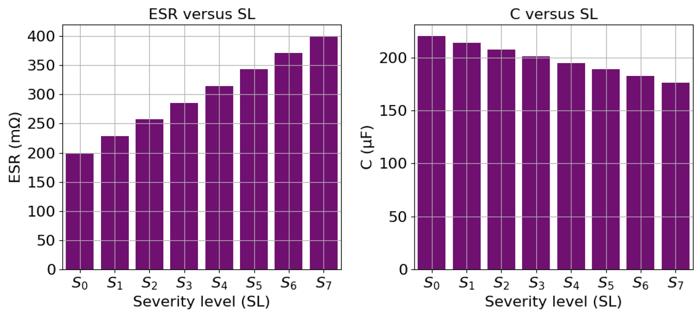
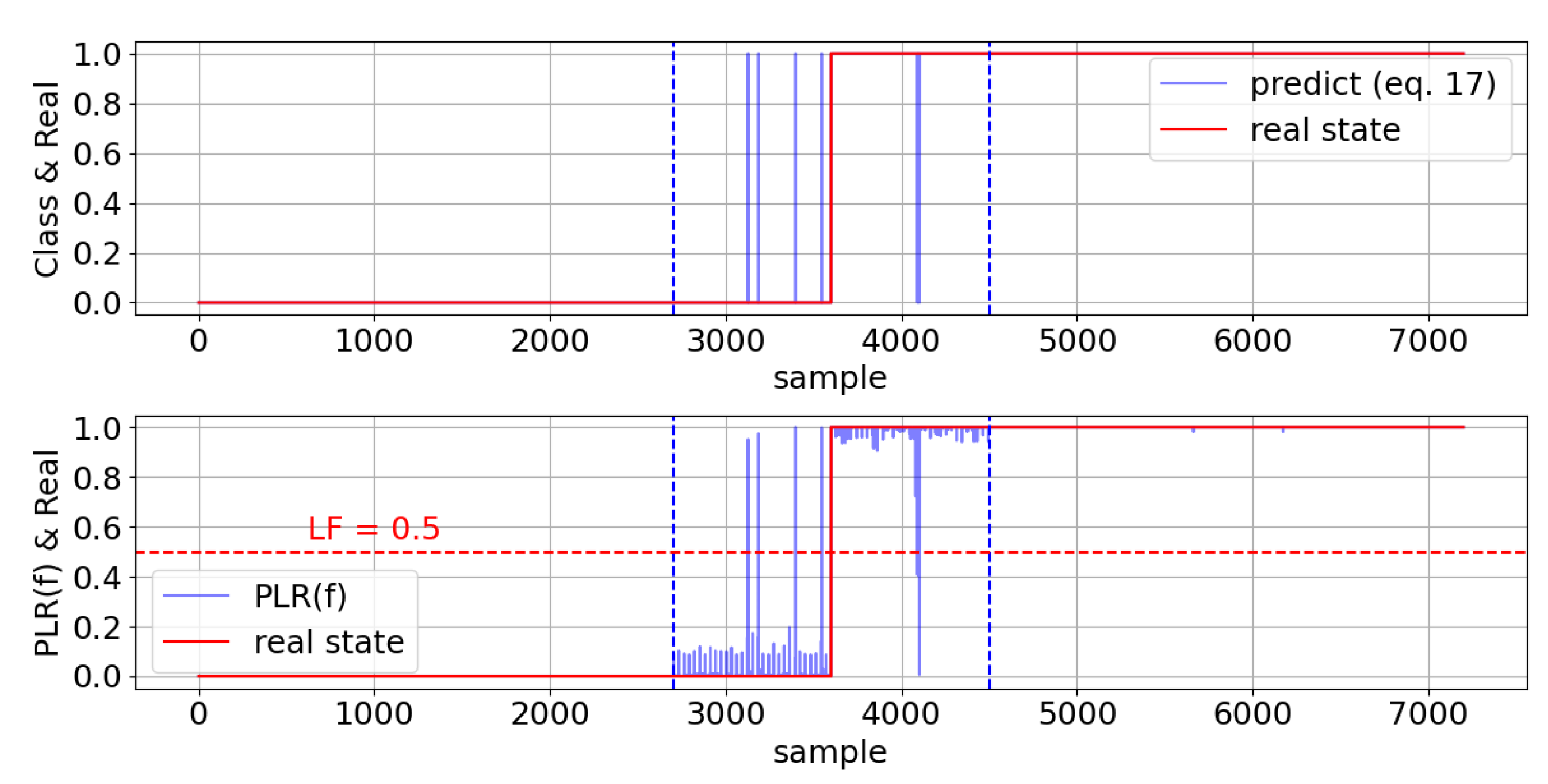
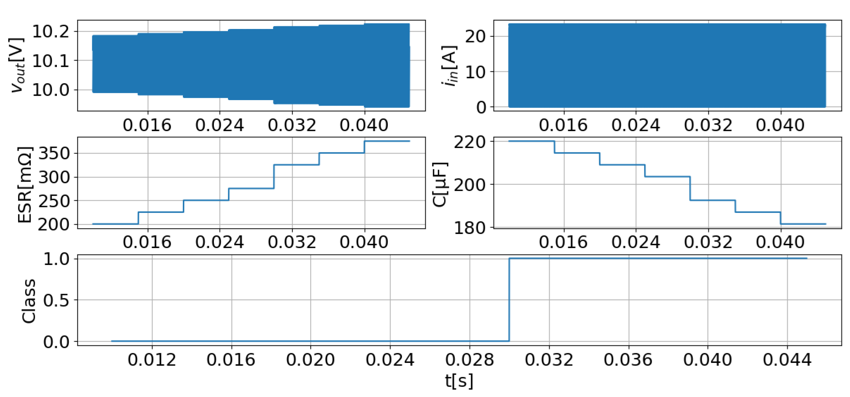
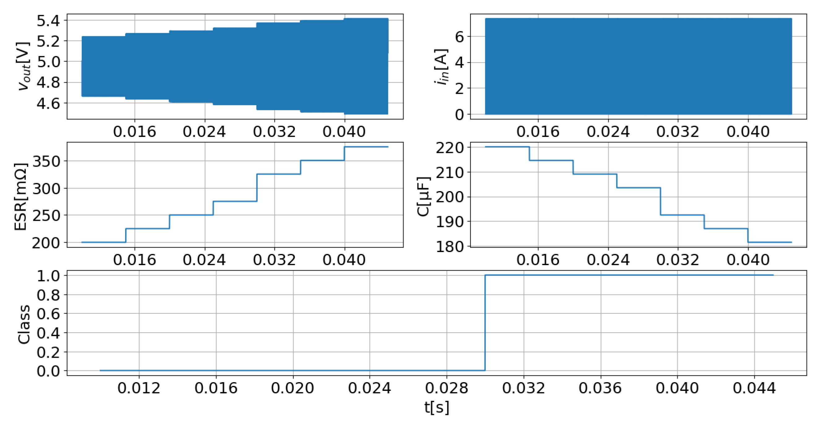
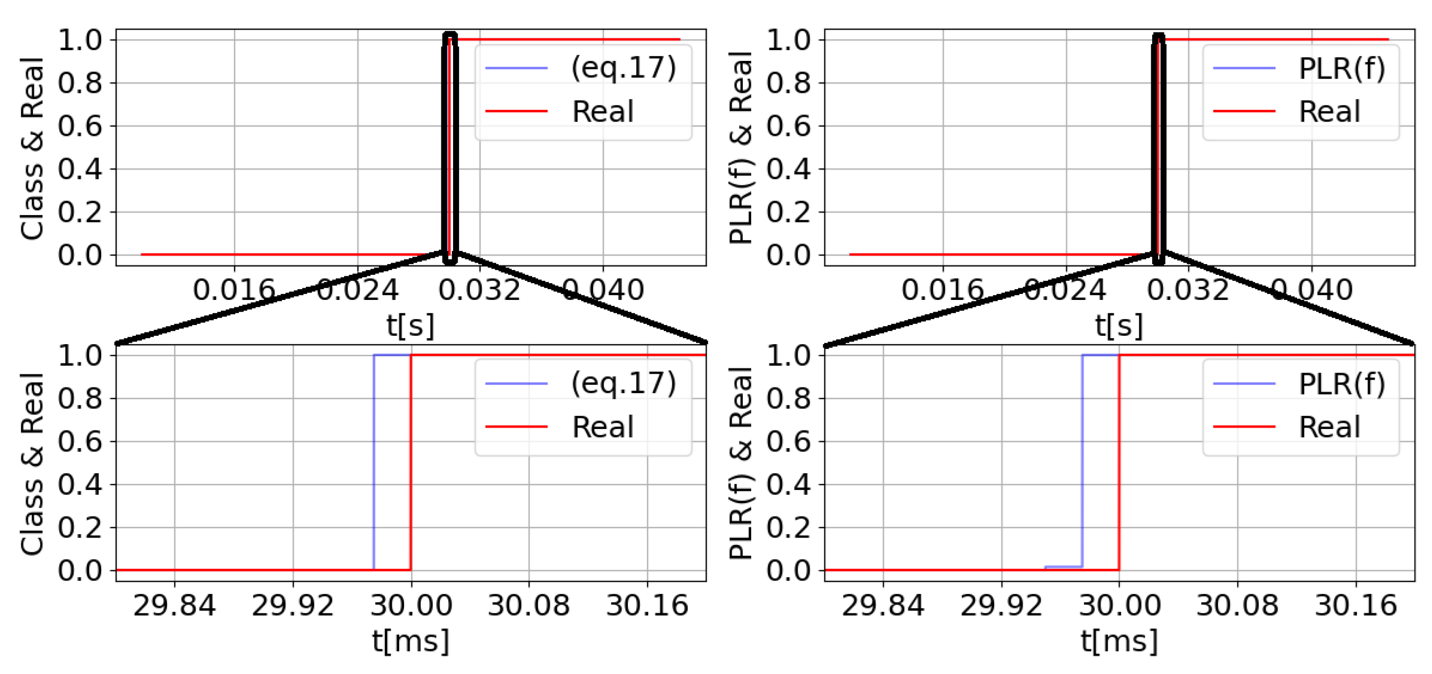
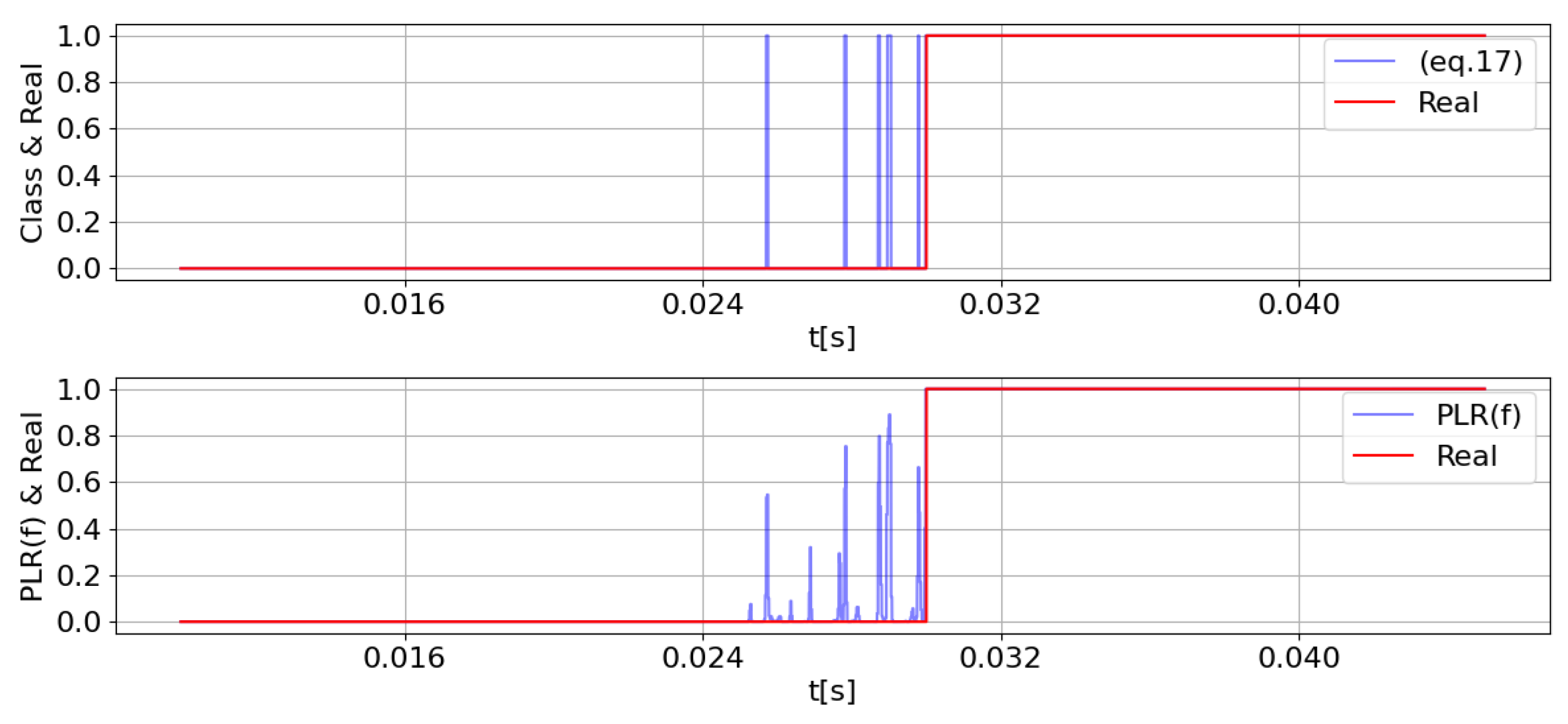
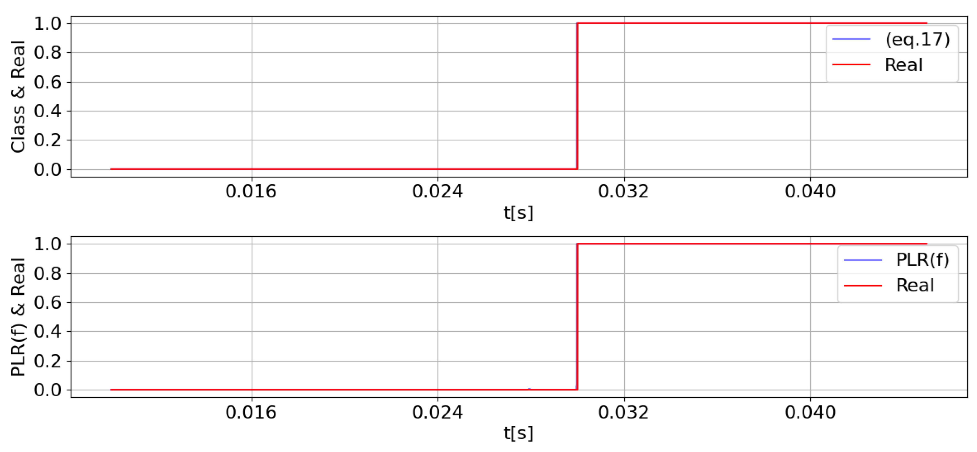
6.1. FDT Assessment in a Buck Converter Under Progressive Al-Cap Deterioration

In this section, the proposed FDT is applied to a buck converter with progressive al-cap degradation. Therefore, to facilitate the analysis, two different scenarios are considered:

• Scenario 1—the electrical specifications of the converter include {v_in = 12 V, L = 44 μH, D = 0.888 and R = 0.444 Ω;
• Scenario 2—the electrical specifications of the converter include {v_in = 12 V, L = 44 μH, D = 0.444 and R = 0.888 Ω.

Each scenario includes six different severity levels applied over specific time periods. Both the scenarios and severity levels are novel to the model and are summarized in

Table 1. Defined scenarios for time-based operation of the buck converter.

Scenario	D	R	t = 15 ms	t = 20 ms	t = 25 ms	t = 30 ms	t = 35 ms	t = 40 ms
1	0.888	0.444	ESR1	ESR2	ESR3	ESR4	ESR5	ESR6
			C1	C2	C3	C4	C5	C6
2	0.444	0.888	ESR1	ESR2	ESR3	ESR4	ESR5	ESR6
			C1	C2	C3	C4	C5	C6

ESR₁ = 225 mΩ; ESR₂ = 250 mΩ; ESR₃ = 275 mΩ; ESR₄ = 325 mΩ; ESR₅ = 350 mΩ; ESR₆ = 375 mΩ; C₁ = 214.5 μF; C₂ = 209 μF; C₃ = 203.5 μF; C₄ = 192.5 μF; C₅ = 187 μF; C₆ = 181.5 μF.

.

Figure 22 presents the waveforms of the output voltage (v_out) and input current (i_in), along with the time-dependent variations in the ESR, C, and corresponding capacitor condition (Class), for Scenario 1, which is described in Table 1.

Figure 23 shows the response of the proposed model (17) to the variations introduced in Scenario 1.

Figure 23 clearly demonstrates the excellent performance of the proposed model, with only incorrect predictions occurring between 29.95 ms and 30 ms. This deviation can be attributed to the ESR and C values being very close to the threshold values (275 mΩ ≈ 300 mΩ and 203.5 μF ≈ 198 μF).

Figure 24 presents the waveforms of the output voltage (v_out) and input current (i_in), along with the time-dependent variations in the ESR, C, and corresponding capacitor condition (Class), for Scenario 2, which is described in Table 1.

Figure 25 shows the response of the proposed model (17) to the variations introduced in Scenario 2.

Similar to Scenario 1, the proposed model exhibits excellent performance in Scenario 2, as shown in Figure 25. In this case, the duration of incorrect predictions is slightly shorter, occurring between 29.97 ms and 30 ms. The cause of this prediction error remains consistent with the previously discussed explanation: the ESR and C values, during this interval, are very close to their respective threshold levels.

It is noteworthy that, in both Scenario 1 and Scenario 2, the recall value is 1, which indicates that the model successfully identified all instances where the capacitor exceeded the replacement threshold. Regarding precision and accuracy, both exhibit values above 0.995, which suggests that the model generates very few false positives and further supports the conclusion that its performance is very good.

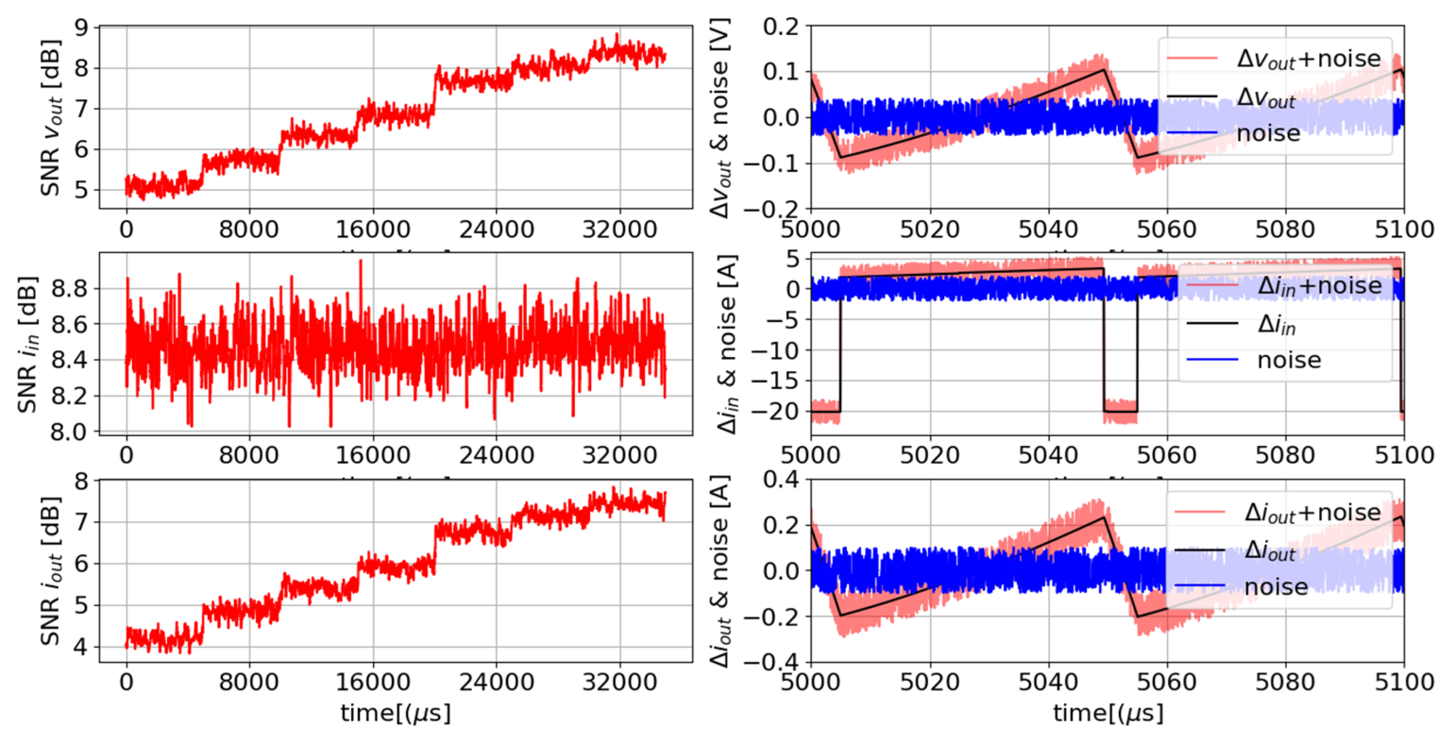
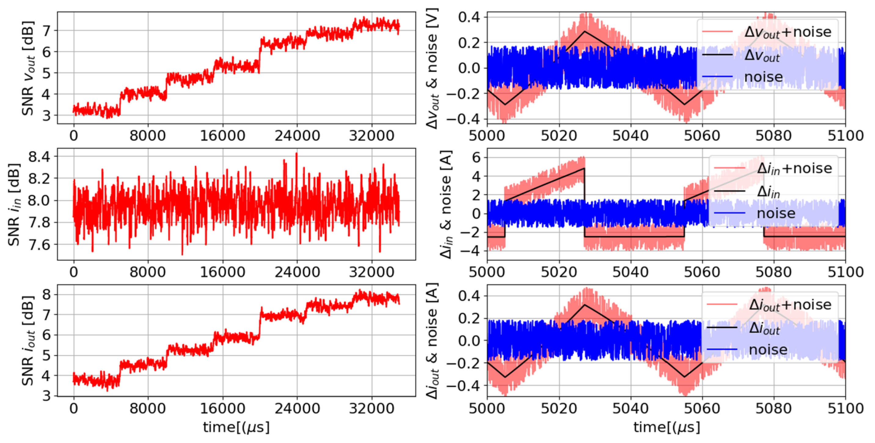
6.2. Robustness Analysis: Model Performance in Noisy Environments

In order to evaluate the applicability of the proposed solution in real-world applications, the FDT is evaluated under very severe noise conditions. The scenarios from Table 1 are repeated with SPM input signals (i_in, i_out, and v_out) that are corrupted by white noise, which achieves a signal–to-noise ratio (SNR) value below 10 dB. SNR values are calculated using the signals’ switching frequency spectral component as the reference signal (i_inAC, i_outAC, and v_outAC).

Figure 26 shows the SNR values for Scenario 1, along with the input signals’ ripple (Δi_in, Δi_out, and Δv_out) under both noisy and noise-free conditions, and the noise component itself.

Figure 27 presents the response of the proposed model (17) to the noisy input signals depicted in Figure 26.

Figure 27 illustrates the robust performance of model (17), even under highly noisy conditions, as demonstrated by a recall of 1.0, an accuracy greater than 0.99, a precision exceeding 0.98, and an F1 score of 0.99.

Scenario 2 is analyzed following the procedure established for Scenario 1. Therefore, Figure 28 shows the SNR values for Scenario 2, along with the input signals’ ripple (Δi_in, Δi_out, and Δv_out) under both noisy and noise-free conditions, and the noise component itself.

Figure 29 presents the response of the proposed model (17) to the noisy input signals depicted in Figure 28.

Figure 29 confirms excellent model robustness under noisy conditions, with the model achieving perfect recall (1.0) and accuracy, precision, and F1 scores greater than 0.99.

7. Scalability of the Proposed Solution

In order to evaluate the scalability of the proposed solution, it was implemented in a boost converter, the circuit topology of which differs from that of the buck converter. Therefore, it was first necessary to adapt the approach presented in [59] to allow the simulation of the boost converter in Python, which was later validated using LTspice.

Then, the same methodology that was applied to the buck converter was executed. A new dataset was generated, consisting of 625 distinct operating conditions (Figure 30) and eight distinct severity levels (Figure 6), resulting in a total of 625 × 8 = 5000 samples (Figure 31).

After the feature selection described in Section 5.1, the data were normalized using Equation (4). Next, in order to evaluate the performance of the proposed solution, model (8) was trained and tested on the full dataset (Figure 31) in 100 independent runs. In each run, 20% of the original samples were randomly selected for training, while the remaining 80%, never observed by the models, were used for testing. The training and testing sets differed in each evaluation. The results of the 100 models are shown in Figure 32.

The average value of the performance metrics across the 100 models exceeded 99.5%, which demonstrated that the proposed solution is scalable to converters with different topologies.

The buck converter generates a DC output voltage lower than the DC input voltage and produces high input current ripple, while the boost converter provides a DC output voltage higher than the DC input voltage with reduced input current ripple. Despite these fundamental topological and operational differences, the proposed solution maintained robust performance, with all four-performance metrics reaching excellent values in all scenarios that were analyzed, regardless of the converter topology and the presence of noise.

8. Conclusions

Energy sustainability is a fundamental goal for modern societies, driven by the increasingly massive use of electricity, particularly from renewable sources.

However, the widespread use of electricity across various sectors is only achievable through power converters, which contain a particularly vulnerable component: the capacitor. Therefore, it is crucial to design fault diagnosis techniques (FDTs) that can evaluate the health status of capacitors to prevent financial losses due to unexpected shutdowns and minimize potential risks to human safety.

Capacitor aging is a gradual process, marked by an increase in internal resistance and a decrease in capacitance. However, once a certain level of degradation is reached, the risk of catastrophic failure, such as an open circuit, rises significantly. This makes it essential to pinpoint the optimal time for replacement.

This paper introduces a non-invasive, data-driven FDT that determines the optimal time for replacing the capacitor in the output filter of a buck converter. The proposed solution integrates a signal processing module (SPM) that extracts attributes from raw data, which are then fed into the information processing module (IPM). The IPM uses these attributes to assess the capacitor’s condition by applying a machine learning algorithm, the logistic regression model that was trained on 20% of the dataset and tested on the remaining 80%. To enhance the computational efficiency and reduce the risk of overfitting, feature selection was employed. Additionally, cross-validation was conducted during the training phase to validate the relevance of the selected features. The model showed outstanding results on both the training and test datasets, with accuracy, precision, recall, and F1 score all exceeding 0.998.

Further validation involved two distinct analyses: evaluation on an independent dataset and real-time implementation during capacitor aging. The former yielded accuracy, precision, recall, and F1 scores greater than 0.99, whereas real-time operation during capacitor degradation sustained comparable performance with all metrics above 0.995.

Additionally, to evaluate the performance of the proposed FDT in real-world applications, the proposed solution was tested in particularly noisy environments, whose signals of interest have SNR levels below 10 dB. Even under these extreme conditions, the proposed solution maintained excellent performance, achieving an accuracy, precision, recall, and F1 score exceeding 0.98.

The proposed solution is well suited for microcontroller implementation due to its low computational requirements and sensor-free operation. Additionally, it was successfully implemented across two different converters, which demonstrated its adaptability and scalability.

Future work will involve implementing the proposed solution in an experimental buck converter prototype. Furthermore, the suitability of the proposed approach will be assessed for other DC-link applications, including power factor correction (PFC), adjustable speed drives (ASDs), and photovoltaic (PV) inverters.

References

1. Eurostat. Energy Statistics—An Overview. 2024. Available online: https://ec.europa.eu/eurostat/statistics-explained/index.php?title=Energy_statistics_-_an_overview (accessed on 2 May 2025).
2. Electricity 2024-Analysis and Forecast to 2026; IEA Publications: Paris, France, 2024.
3. Scolaro, E.; Beligoj, M.; Estevez, M.; Alberti, L.; Mattetti, M.R.E.M. Electrification of Agricultural Machinery: A Review. IEEE Access 2021, 9, 164520–164541. [Google Scholar] [CrossRef]
4. Ahmed, B.; Shabbir, H.; Naqvi, S.R.; Peng, L. Smart Agriculture: Current State, Opportunities, and Challenges. IEEE Access 2024, 12, 144456–144478. [Google Scholar] [CrossRef]
5. Meng, L.; Hirayama, T.; Oyanagi, S. Underwater-Drone with Panoramic Camera for Automatic Fish Recognition Based on Deep Learning. IEEE Access 2018, 6, 17880–17886. [Google Scholar] [CrossRef]
6. Industrial Electrification. International Institute for Sustainable Development. 2022. Available online: https://www.iisd.org/system/files/2022-05/industrial-electrification-en.pdf (accessed on 2 May 2025).
7. Borgosano, S.; Martini, D.; Longo, M.; Foiadelli, F. Electrifying Urban Transportation: A Comparative Study of Battery Swap Stations and Charging Infrastructure for Taxis in Chicago. IEEE Access 2024, 12, 48017–48026. [Google Scholar] [CrossRef]
8. Silva, C.; Peres, L. Introducing Electric Bus Fleets in Rio de Janeiro City Methodology and Analysis. IEEE Lat. Am. Trans. 2022, 20, 2087–2095. [Google Scholar] [CrossRef]
9. Yang, G.; Ye, Z.; Wu, H.; Li, C.; Wang, R.; Hou, D.; Huang, H.W.X.; Pang, Z.; Dong, N.; Pang, G. A Digital Twin-Based Large-Area Robot Skin System for Safer Human-Centered Healthcare Robots Toward Healthcare 4.0. IEEE Trans. Med. Robot. Bionics 2024, 6, 1104–1115. [Google Scholar] [CrossRef]
10. Ma, B.; Kuo, Y.; Jiang, Y.; Huang, G. RubikCell: Toward Robotic Cellular Warehousing Systems for E-Commerce Logistics. IEEE Trans. Eng. Manag. 2024, 71, 9270–9285. [Google Scholar] [CrossRef]
11. Costa, L.; Liserre, M. Failure Analysis of the dc-dc Converter: A Comprehensive Survey of Faults and Solutions for Improving Reliability. IEEE Power Electron. Mag. 2018, 5, 42–51. [Google Scholar] [CrossRef]
12. Azrul, M.H.S.E.M.; Mashohor, S.; Amran, M.E.; Hafiz, N.F.; Ali, A.M.; Naseri, M.S.; Rasid, M.F.A. Assessment of IoT-Driven Predictive Maintenance Strategies for Computed Tomography Equipment: A Machine Learning Approach. IEEE Access 2024, 12, 195505–195515. [Google Scholar]
13. SRahimpour; Husev, O.; Vinnikov, D.; Kurdkandi, N.V.; Tarzamni, H. Fault Management Techniques to Enhance the Reliability of Power Electronic Converters: An Overview. IEEE Access 2023, 11, 13432–13446. [Google Scholar] [CrossRef]
14. Cardoso, A.J.M. Diagnosis and Fault Tolerance of Electrical Machines, Power Electronics and Drives; The Institution of Engineering and Technology: Stevenage, UK, 2018. [Google Scholar]
15. Amaral, A.M.R.; Cardoso, A.J.M. An Economic Offline Technique for Estimating the Equivalent Circuit of Aluminum Electrolytic Capacitors. IEEE Trans. Instrum. Meas. 2008, 57, 2697–2710. [Google Scholar] [CrossRef]
16. Agarwal, N.; Ahmad, M.W.; Anand, S. Quasi-Online Technique for Health Monitoring of Capacitor in Single-Phase Solar Inverter. IEEE Trans. Power Electron. 2018, 33, 5283–5291. [Google Scholar] [CrossRef]
17. Amaral, A.M.R.; Laadjal, K.; Cardoso, A.J.M. Advancements in Fault Diagnosis Techniques for Aluminum Capacitors Using STLSP and Autoencoder. In Proceedings of the IEEE International Conference on Artificial Intelligence & Green Energy (ICAIGE), Yasmine Hammame, Tunisia, 10–12 October 2024. [Google Scholar]
18. Gao, Z.; Cecati, C.; Ding, S.X. A Survey of Fault Diagnosis and Fault-Tolerant Techniques—Part I: Fault Diagnosis with Model-Based and Signal-Based Approaches. IEEE Trans. Ind. Electron. 2015, 62, 3757–3767. [Google Scholar] [CrossRef]
19. Amaral, A.; Laadjal, K.; Cardoso, A.J.M. Optimized Preventive Diagnostic Algorithm for Assessing Aluminum Electrolytic Capacitor Condition Using Discrete Wavelet Transform and Kalman Filter. Electronics 2024, 13, 3265. [Google Scholar] [CrossRef]
20. Kumar, G.K.; Elangovan, D. Review on fault-diagnosis and fault-tolerance for DC–DC converters. IET Power Electron. 2020, 13, 1–13. [Google Scholar] [CrossRef]
21. Amaral, A.M.R.; Cardoso, A.J.M. Simulation Tool to Evaluate Fault Diagnosis Techniques for DC-DC Converters. Symmetry 2022, 14, 1886. [Google Scholar] [CrossRef]
22. Nichicon Corporation. General Descriptions of Aluminum Electrolytic Capacitors-Technical Notes CAT.8101E-1. Available online: https://www.nichicon.co.jp/english/products/pdf/aluminum-e.pdf (accessed on 18 April 2025).
23. Guide, S. Technical Guide: Aluminum Electrolytic Capacitor, Conductive Polymer Hybrid Aluminum and Electrolytic Capacitor; Panasonic Industry: Osaka, Japan, 2024. [Google Scholar]
24. Ho, J.; Jow, T.; Boggs, S. Historical introduction to capacitor technology. IEEE Electr. Insul. Mag. 2010, 26, 20–25. [Google Scholar] [CrossRef]
25. Amaral, A.M.R.; Laadjal, A.K.; Cardoso, J.M. Assessment of Aluminum Electrolytic Capacitors Health Status Through Signal-Based Techniques. In Proceedings of the IEEE 21st International Power Electronics and Motion Control Conference (PEMC), Pilsen, Czech Republic, 30 September–3 October 2024. [Google Scholar]
26. Dubilier, C.C. Aluminum Electrolytic Capacitor Application Guide. Available online: https://www.cde.com/resources/technical-papers/KNO_CD_AEappGuide_R2.pdf (accessed on 1 May 2025).
27. Harada, K.; Katsuki, A.; Fujiwara, M. Use of ESR for deterioration diagnosis of electrolytic capacitor. IEEE Trans. Power Electron. 1993, 8, 355–361. [Google Scholar] [CrossRef]
28. Amaral, A.M.R.; Cardoso, A.J.M. Fault diagnosis on switch-mode power supplies operating in discontinuous mode. In Proceedings of the Second International Conference on Power Electronics, Machines and Drives (PEMD 2004), Edinburgh, UK, 21–23 September 2004. [Google Scholar]
29. Amaral, A.M.R.; Cardoso, A.J.M. Using input current and output voltage ripple to estimate the output filter condition of switch mode DC/DC converters. In Proceedings of the IEEE International Symposium on Diagnostics for Electric Machines, Power Electronics and Drives, Cargese, France, 31 August–3 September 2009. [Google Scholar]
30. Aeloiza, E.; Kim, J.-H.; Enjeti, P.; Ruminot, P. A Real Time Method to Estimate Electrolytic Capacitor Condition in PWM Adjustable Speed Drives and Uninterruptible Power Supplies. In Proceedings of the IEEE 36th Power Electronics Specialists Conference, Dresden, Germany, 12–16 June 2005. [Google Scholar]
31. Venet, P.; Perisse, F.; El-Husseini, M.H.; Rojat, G. Realization of a smart electrolytic capacitor circuit. IEEE Ind. Appl. Mag. 2002, 8, 16–20. [Google Scholar] [CrossRef]
32. Amaral, A.M.R.; Cardoso, A.J.M. State condition estimation of aluminum electrolytic capacitors used on the primary side of ATX power supplies. In Proceedings of the 35th Annual Conference of IEEE Industrial Electronics, Porto, Portugal, 3–5 November 2009. [Google Scholar]
33. Sundararajan, P.; Sathik, M.; Sasongko, F.; Tan, C.; Pou, J.; Blaabjerg, F. Condition Monitoring of DC-Link Capacitors Using Goertzel Algorithm for Failure Precursor Parameter and Temperature Estimation. IEEE Trans. Power Electron. 2020, 35, 6386–6396. [Google Scholar] [CrossRef]
34. Amaral, A.M.R.; Laadjal, K.; Cardoso, A.J.M. Enhanced DC-link Capacitors Failure Diagnosis for a Three-Phase Interleaved Converter, Using Hilbert Transform. In Proceedings of the IEEE 21st International Power Electronics and Motion Control Conference (PEMC), Pilsen, Czech Republic, 30 September–3 October 2024. [Google Scholar]
35. Wang, G.; Guan, Y.; Zhang, J.; Wu, L.; Zheng, X.; Pan, W. ESR estimation method for DC-DC converters based on improved EMD algorithm. In Proceedings of the IEEE 2012 Prognostics and System Health Management Conference, Beijing, China, 23–25 May 2012. [Google Scholar]
36. Chen, Z.; Lin, Q.; Yu, K.; Su, X.; Du, W. A Non-invasive Online ESR Estimating Method for DC-Link Capacitors of UPS. In Proceedings of the 4th International Conference on Smart Power & Internet Energy Systems (SPIES), Beijing, China, 27–30 October 2022. [Google Scholar]
37. Ren, L.; Gong, C.; Zhao, Y. An Online ESR Estimation Method for Output Capacitor of Boost Converter. IEEE Trans. Power Electron. 2019, 34, 10153–10165. [Google Scholar] [CrossRef]
38. Ma, H.; Mao, X.; Zhang, N.; Xu, D. Parameter Identification of Power Electronic Circuits Based on Hybrid Model. In Proceedings of the IEEE 36th Power Electronics Specialists Conference, Recife, Brazil, 12–16 June 2005. [Google Scholar]
39. Buiatti, G.M.; Amaral, A.M.R.; Cardoso, A.J.M. ESR Estimation Method for DC/DC Converters Through Simplified Regression Models. In Proceedings of the IEEE Industry Applications Annual Meeting, New Orleans, LA, USA, 23–27 September 2007. [Google Scholar]
40. Buiatti, G.M.; Amaral, A.M.R.; Cardoso, A.J.M. Parameter Estimation of a DC/DC Buck converter using a continuous time model. In Proceedings of the European Conference on Power Electronics and Applications, Aalborg, Denmark, 2–5 September 2007. [Google Scholar]
41. Buiatti, G.M.; Amaral, A.M.R.; Cardoso, A.J.M. An Online Technique for Estimating the Parameters of Passive Components in Non-Isolated DC/DC Converters. In Proceedings of the IEEE International Symposium on Industrial Electronics, Vigo, Spain, 4–7 June 2007. [Google Scholar]
42. Buiatti, G.M.; Amaral, A.M.R.; Cardoso, A.J.M. An unified method for estimating the parameters of non-isolated DC/DC converters using continuous time models. In Proceedings of the 29th International Telecommunications Energy Conference, Rome, Italy, 30 September–4 October 2007. [Google Scholar]
43. Peng, Y.; Wang, H. Application of Digital Twin Concept in Condition Monitoring for DC-DC Converter. In Proceedings of the IEEE Energy Conversion Congress and Exposition (ECCE), Baltimore, MD, USA, 29 September–3 October 2019. [Google Scholar]
44. Soliman, H.; Wang, H.; Gadalla, B.; Blaabjerg, F. Condition monitoring for DC-link capacitors based on artificial neural network algorithm. In Proceedings of the IEEE 5th International Conference on Power Engineering, Energy and Electrical Drives (POWERENG), Riga, Latvia, 11–13 May 2015. [Google Scholar]
45. Soliman, H.; Abdelsalam, I.; Wang, H.; Blaabjerg, F. Artificial Neural Network based DC-link capacitance estimation in a diode-bridge front-end inverter system. In Proceedings of the IEEE 3rd International Future Energy Electronics Conference and ECCE Asia, Kaohsiung, Taiwan, 3–7 June 2017. [Google Scholar]
46. Soliman, H.; Davari, P.; Wang, H.; Blaabjerg, F. Capacitance estimation algorithm based on DC-link voltage harmonics using artificial neural network in three-phase motor drive systems. In Proceedings of the IEEE Energy Conversion Congress and Exposition (ECCE), Cincinnati, OH, USA, 1–5 October 2017. [Google Scholar]
47. Kamel, T.; Biletskiy, Y.; Chang, L. Capacitor aging detection for the DC filters in the power electronic converters using ANFIS algorithm. In Proceedings of the IEEE 28th Canadian Conference on Electrical and Computer Engineering, Halifax, NS, Canada, 3–6 May 2015. [Google Scholar]
48. Apsari, D.; Lee, D. Capacitance and ESR Estimation of DC-link Capacitors in AC Machine Drives Based on Hybrid CNN-Attention Model. In Proceedings of the IEEE 10th International Power Electronics and Motion Control Conference, Chengdu, China, 17–20 May 2024. [Google Scholar]
49. Rajendran, S.; Jena, D.; Diaz, M.; Devi, V.S.K. Machine learning based condition monitoring of a DC-link capacitor in a Back-to-Back converter. In Proceedings of the IEEE International Conference on Automation/XXV Congress of the Chilean Association of Automatic Control (ICA-ACCA), Curicó, Chile, 24–28 October 2022. [Google Scholar]
50. McGrew, T.; Sysoeva, V.; Cheng, C.H.; Miller, C.; Scofield, J.; Scott, M.J. Condition Monitoring of DC-Link Capacitors Using Time–Frequency Analysis and Machine Learning Classification of Conducted EMI. IEEE Trans. Power Electron. 2022, 37, 12606–12618. [Google Scholar] [CrossRef]
51. Amaral, A.M.R.; Laadjal, K.; ACardoso, J.M. Advanced Fault-Detection Technique for DC-Link Aluminum Electrolytic Capacitors Based on a Random Forest Classifier. Electronics 2023, 12, 2572. [Google Scholar] [CrossRef]
52. Amaral, A.M.R.; Laadjal, K.; Cardoso, A.J.M. Assessment of the Integrity of Aluminum Electrolytic Capacitors Using a Logistic Regression Model. In Proceedings of the IEEE International Conference on Artificial Intelligence & Green Energy (ICAIGE), Yasmine Hamm, Tunisia, 10–12 October 2024. [Google Scholar]
53. Kareem, A.; Basheer, V.; Kumara, V. A Second-Order Sliding Mode Control Scheme with Fuzzy Logic-Based Online Sliding Surface Adjustment for Buck Converters. IEEE Access 2025, 13, 48792–48801. [Google Scholar] [CrossRef]
54. Subedi, S.; Gui, Y.; Xue, Y. Applications of Data-Driven Dynamic Modeling of Power Converters in Power Systems: An Overview. IEEE Trans. Ind. Appl. 2025, 61, 2434–2456. [Google Scholar] [CrossRef]
55. Venkatramanan, D.; John, V. Dynamic Modeling and Analysis of Buck Converter Based Solar PV Charge Controller for Improved MPPT Performance. IEEE Trans. Ind. Appl. 2019, 55, 6234–6246. [Google Scholar] [CrossRef]
56. Mammeri, E.; Santos, O.; Aroudi, A.; Domajnko, J.; Prosen, N.; Salamero, L. Modeling and Control of a Three-Phase Interleaved Buck Converter as a Battery Charger. IEEE Access 2025, 13, 18325–18345. [Google Scholar] [CrossRef]
57. Kim, J.; Yoon, J.; Choi, B. A High-Light-Load-Efficiency Low-Ripple-Voltage PFM Buck Converter for IoT Applications. IEEE Trans. Power Electron. 2022, 37, 5763–5772. [Google Scholar] [CrossRef]
58. Park, W.; Namgoong, G.; Choi, E.; Lee, B.; Park, H.; Ma, H.; Bien, F. A 94% Peak Efficiency Dual Mode Buck Converter with Fully Integrated On-Time-Based Mode Control for Implantable Medical Devices. IEEE Trans. Circuits Syst. II Express Briefs 2022, 69, 4458–4462. [Google Scholar] [CrossRef]
59. Amaral, A.M.R.; Cardoso, A.J.M. Using Python for the Simulation of a Closed-Loop PI Controller for a Buck Converter. Signals 2022, 3, 313–325. [Google Scholar] [CrossRef]
60. Giesselmann, M.; Roy, V. Modeling of power supplies for power modulators with LTspice. IEEE Trans. Dielectr. Electr. Insul. 2019, 26, 508–514. [Google Scholar] [CrossRef]
61. Jović, A.; Brkić, K.; Bogunović, N. A review of feature selection methods with applications, 2015. In Proceedings of the 38th International Convention on Information and Communication Technology, Electronics and Microelectronics (MIPRO), Opatija, Croatia, 25–29 May 2015. [Google Scholar]
62. Nasir, I.M.; Khan, M.; Yasmin, M.; Shah, J.; Gabryel, M.; Scherer, R.; Damasevicius, R. Pearson Correlation-Based Feature Selection for Document Classification Using Balanced Training. Sensors 2020, 20, 6793. [Google Scholar] [CrossRef] [PubMed]
63. Njimbouom, S.; Lee, K.; Lee, H.; Kim, J. Predicting Site Energy Usage Intensity Using Machine Learning Models. Sensors 2023, 23, 82. [Google Scholar] [CrossRef] [PubMed]
64. Wang, W.; Lu, L.; Wei, W. A Novel Supervised Filter Feature Selection Method Based on Gaussian Probability Density for Fault Diagnosis of Permanent Magnet DC Motors. Sensors 2022, 22, 7121. [Google Scholar] [CrossRef]
65. Supurtulu, M.; Hatipoglu, A.; Yılmaz, E. An Analytical Benchmark of Feature Selection Techniques for Industrial Fault Classification Leveraging Time-Domain Features. Appl. Sci. 2025, 15, 1457. [Google Scholar] [CrossRef]
Figure 1. Basic structure of an al-cap [22]: (a) the whole structure and (b) inside the can.
Applsci 15 06971 g001
Figure 2. Simplified equivalent circuit of an al-cap [14].
Applsci 15 06971 g002
Figure 3. Buck converter schematics.
Applsci 15 06971 g003
Figure 4. Signal processing module (SPM): primary feature extraction pipeline.
Applsci 15 06971 g004
Figure 5. Range of randomly defined operating conditions, where R denotes the load resistance and D the duty cycle.
Applsci 15 06971 g005
Figure 6. Severity levels versus ESR and C values.
Applsci 15 06971 g006
Figure 7. Complete dataset used to train and test the machine learning models.
Applsci 15 06971 g007
Figure 8. Individual boxplots regarding the features.
Applsci 15 06971 g008
Figure 9. Correlation among all features.
Applsci 15 06971 g009
Figure 10. Mutual information between the features and the target (ranked by their relevance).
Applsci 15 06971 g010
Figure 11. Fisher score by feature regarding each class (ranked by their relevance).
Applsci 15 06971 g011
Figure 12. Final dataset after feature normalization.
Applsci 15 06971 g012
Figure 13. Training dataset (TrainDS).
Applsci 15 06971 g013
Figure 14. Assessment of model performance during cross-validation.
Applsci 15 06971 g014
Figure 15. Evaluation results for 100 distinct LR models, each trained on 20% of the dataset (Figure 12) and tested on the remaining 80%.
Applsci 15 06971 g015
Figure 16. Evaluation results for 100 distinct DT models, each trained on 20% of the dataset (Figure 12) and tested on the remaining 80%.
Applsci 15 06971 g016
Figure 17. Model (17)’s response to the entire dataset (Figure 12).
Applsci 15 06971 g017
Figure 18. Randomly defined range of operating conditions for the test dataset.
Applsci 15 06971 g018
Figure 19. Severity levels versus ESR and C values for the test dataset.
Applsci 15 06971 g019
Figure 20. Test dataset used during deployment phase.
Applsci 15 06971 g020
Figure 21. Model (Equation (17)) response to the dataset presented in Figure 20.
Applsci 15 06971 g021
Figure 22. Converter output voltage (vout) and input current (iin), along with time-dependent variations in ESR, C and corresponding capacitor condition (Class) for Scenario 1, described in Table 1.
Applsci 15 06971 g022
Figure 23. Response of the proposed model (17) to the variations introduced in Scenario 1.
Applsci 15 06971 g023
Figure 24. Converter output voltage (vout) and input current (iin), along with time-dependent variations in ESR, C, and corresponding capacitor condition (Class), for Scenario 2 described in Table 1.
Applsci 15 06971 g024
Figure 25. Response of the proposed model (17) to the variations introduced in Scenario 2.
Applsci 15 06971 g025
Figure 26. Scenario 1 (Table 1): Input SNR, input signal ripple (Δiin, Δiout, and Δvout) under clean and noisy conditions, and noise component.
Applsci 15 06971 g026
Figure 27. Model (17) performance under noisy input signals (Figure 26).
Applsci 15 06971 g027
Figure 28. Scenario 2 (Table 1): Input SNR, input signal ripple (Δiin, Δiout, and Δvout) under clean and noisy conditions, and noise component.
Applsci 15 06971 g028
Figure 29. Model (17) performance under noisy input signals (Figure 27).
Applsci 15 06971 g029
Figure 30. Range of randomly defined operating conditions, regarding the boost converter dataset consisting of 625 distinct operating conditions, where R denotes the load resistance and D the duty cycle. The values of vin (5 V) and L (44 μH) are kept constant throughout all simulations.
Applsci 15 06971 g030
Figure 31. Boost converter dataset, derived from 5000 simulations, containing all primary features, ESR, C, and target variable (class or capacitor Status).
Applsci 15 06971 g031
Figure 32. Evaluation results for 100 distinct LR models, each trained on 20% of the dataset (Figure 31) and tested on the remaining 80%.
Applsci 15 06971 g032