1. Introduction
The management of onboard systems and health status monitoring of a spacecraft is a pivotal but extremely wide aspect of satellite design that is being reshaped as satellites evolve and autonomy increases. Onboard Fault Detection, Isolation, and Recovery (FDIR) provides supervision and control on the satellite behavior under unexpected situations and malfunctions. The main design philosophies for carrying the task of anomaly identification onboard spacecrafts, at the current time, are model-based and data-driven. Model-based techniques exploit an “analytical redundancy” of the onboard subsystems: by running an onboard model in parallel with real-time operations as they are performed, the spacecraft relies on a duplicated virtual version of part of itself. By checking simultaneously the outputs of real elements and their simulated version, residuals are periodically calculated, and it is possible to establish if any discrepancy from the expected scenario has occurred. Analytical redundancy adds a layer of cross-checks without the addition of hardware components to the system: the result of these checks shall be translated into a decision function to eventually proceed with the available recovery actions, if necessary [
1]. In the context of CubeSats, Lobo et al. (2019) built an FDIR framework based on analytical redundancy and residual-based logic for fault isolation [
2]. For similar live time-varying signal monitoring, in a more recent work Xu et al. (2025) developed a model-based approach which utilizes input-compensated recursive least squares and disturbance observers, for a robust inverter fault diagnosis through parameters estimation [
3]. Data-driven algorithms, on the other hand, can work with live acquired data, ranging from housekeeping parameters to raw sensor output, to notify the spacecraft and flight engineers when some anomalous behavior is detected [
4]. By exploiting knowledge on process history, it is possible to notice novel or unusual behavior even without an explicit model of the system. Both of these philosophies come with potential weaknesses: one of the drawbacks with model-based techniques is the fact that they require sufficiently accurate dynamic models, which must be designed, optimized, and end up consuming a discrete amount of onboard computational resources. Data-driven approaches attempt to specifically overcome this issue while maintaining a high reliability of detection. However, it is clear that the focus must shift to the quality and relevance of training data, and the selection of statistical knowledge used to monitor the system must be extremely well targeted.
Specifically, in the realm of fault detection, the adoption of data-driven methods is widespread and concerns many different fields: surveys such as Chen et al. (2023) gathered useful and reliable diagnostic methods from recent years, in this specific case with a special focus on HVAC systems [
5]. In the current study, attention is drawn on two very common (supervised) Machine Learning approaches for classification, with some meaningful research heritage that hints to potential cutting-edge space applications: Support Vector Machines (SVMs) and Artificial Neural Networks (ANNs). In industrial mechanics, SMVs are already quite popular, with a few examples focusing on fault detection through feature extraction. For instance, Rauber et al. (2014) focused on bearing fault diagnosis [
6], Jan et al. (2017) confirmed the very same extracted features pool for sensor fault diagnosis through SVMs [
7], while Samanta (2004) employed a further optimization of extracted features through a genetic algorithm [
8]. In the space domain, examples are fewer, at least for what concerns fault detection: Gao, Yu et al. (2012) employed principal component analysis and SVMs to classify output data from sensors and actuators, with promising results in all explored cases [
9], while Ding et al. (2021) focused on spacecraft leakage detection through SVMs, also applying a feature ranking algorithm [
10]. Many of the strategies employ sophisticated reduction methods to diminish the size of the input vector, but a lot of these methods do not involve MIL testing, applying classification offline, or do not match up different SVM architectures for comparison in bulk. Support Vector Machines are relatively easy to intuitively comprehend, and can achieve high efficiencies, thanks to the use of kernels [
11]. Support vectors are intended to be used as binary classifiers, but through structured architectures, they have become extremely widespread also for multi-class categorization [
12].
Artificial Neural Networks are slightly less obvious to fully understand theoretically, and their hyper-parameters suffer from a lack of physically meaningful interpretation [
13]; despite this, their use is following a rapid increase in popularity due to high performance for what concerns pattern recognition and classification, especially when exploiting a feature extraction mechanism to select their inputs, much like SVMs. Sorsa et al. (1991) showed 10-class fault classification on a realistic continuous stirred tank reactor system through ANNs [
14], Samanta and Al-Balushi (2001) focused once again on fault diagnostic for rolling element bearings with only five extracted features [
15], while Ma et al. (2023) used networks to apply both detection and diagnosis on high-speed train air brake pipes [
16]. The variety of layer structures and node types is incredibly wide, and therefore, the topic is still under close study and within a heavy experimenting phase [
17]: space applications are many and diversified, and extremely high accuracy in classification problems can be achieved with a multitude of layer setups. Valdes et al. (2009) developed a dynamic Neural Network Fault Detection and Isolation (FDI) framework for pulsed plasma thrusters, with hints to an integrated scheme for combined high and low level FDI [
18], O’Meara et al. (2018) used different Neural Network architectures to perform automatic feature extraction, anomaly detection, and telemetry prediction [
19], and Li et al. approached voltage anomalies detection through a deep belief network architecture [
20]. Once again, many tests are run offline, with no consequential MIL testing: tests in space rarely concern a satellite’s ADCS and only concern a few network architectures, without a critical comparison with other kinds of data-driven methods, such as threshold-based, that could be considered a useful signal monitoring benchmark algorithm. Fault detection and diagnosis through Neural Networks and SVMs is an incredibly wide topic, which is being tackled by dozens of different directions at once, by exploiting the state of the art on both these models. Despite the proven efficacy of Deep Learning solutions for systems’ health monitoring and fault detection, FDIR in space applications still misses a shared standard or universal strategy. In a loosely structured field such as this, especially on the pivotal Attitude Determination and Control Subsystem, Machine Learning is a better choice for what concerns computational resources, fast training, heritage, and most importantly, when the aim is to build a basic but wide comparison of a large range of architectures: for this reason, a rigorous but gradual approach is adopted.
The aim of this research is, starting from a realistic framework in a functional simulator, reproducing an Earth-orbiting satellite’s Attitude Determination and Control System (ADCS), to focus on the analysis of signals onboard the spacecraft and the diagnosis process of faults: the task is to examine performances of a collection of basic detection algorithms employing Machine Learning, in comparison to the architecture of a simple threshold-based data-driven fault detector, to find the most appropriate shape for an enhanced FDIR architecture. Once the problem of a reliable AI-aided detection and diagnosis is tackled, this new paradigm can be extended to other subsystems beyond Guidance, Navigation, and Control (GNC), so that the whole spacecraft, at system level, could eventually benefit from this enhanced robustness.
The remaining chapters of this document are structured as follows:
Section 2 presents an overview of the methodology adopted and the main data-driven techniques explored in this study, from a conceptual point of view. Particular emphasis is placed on describing the specific features extracted in
Section 3. The experimental setup is showcased in all its aspects in
Section 4, alongside details on dataset generation, and the simple algorithm used as a benchmark is described. Finally, AI-based techniques are put to the test in a variety of scenarios in
Section 5: through the comparison with other algorithms, their strengths and weak points suggest their most promising uses, which are further evaluated in specific case studies, explored as a very last investigation.
2. Proposed Methodology of This Study
The aim of this section is to explore the methodology adopted and the underlying concepts of data-driven methods employed, to better understand the reasons behind the main design choices. First of all, an overview on the framework, the setting of the testing environment, and the strategy of data processing are given. Afterwards, some insight on data-driven techniques for detection is presented: firstly, the basic one based on thresholds in
Section 2.1; then, some theoretical background of the main two Machine Learning methods adopted is provided in
Section 2.2 and
Section 2.3, highlighting the reason for their use and their limitations. Finally, in
Section 2.4, most of the typical faults of a satellite’s ADCS are summarized in a restricted number of anomalous scenarios: these are adopted in a modular way as the baseline for building the large datasets employed in this study, for training and simulation purposes.
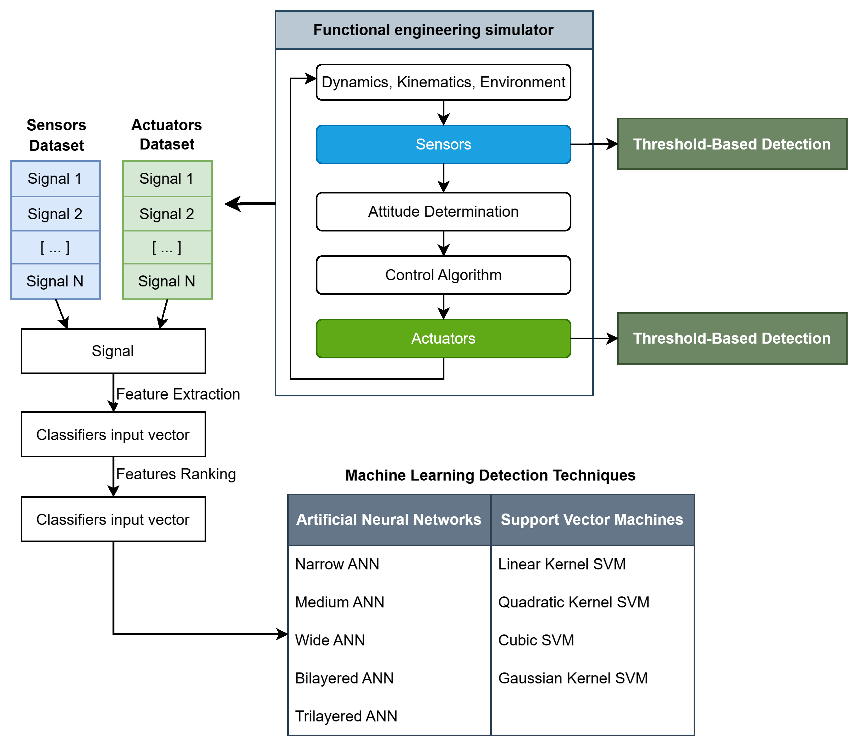
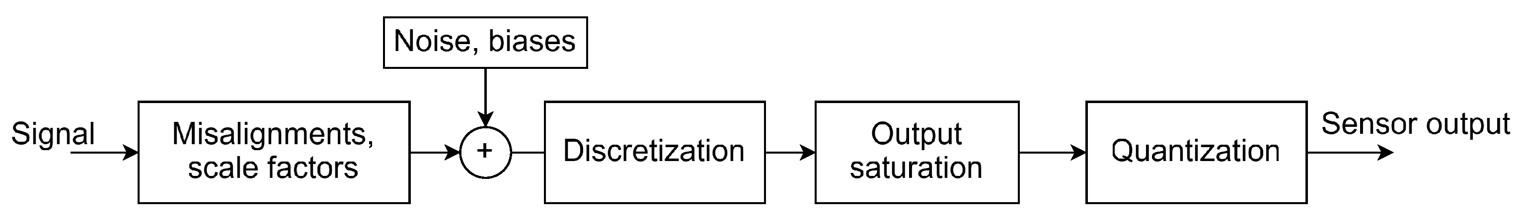
As shown in
Figure 1, two detection methods with radically different approaches are followed: one is a relatively simple variance-based detection algorithm, relying on thresholds and logical relations, which takes data directly from the simulation and is explored in detail in
Section 2.1. The other approach involves the characteristic process pipeline for Machine Learning techniques: data from sensors and actuators is gathered into large datasets containing signal records from hundreds of simulations. Each element of these datasets is then further processed: instead of storing and working with entire signals, only a few time- and frequency-domain features are extracted to significantly reduce the number of inputs for the learning agents to train on. All of the features are explained and motivated in
Section 3, while the full list of employed classifiers is detailed in
Section 5.
This work approaches the use of Machine Learning in fault detection in a spacecraft’s ADCS context, while trying to extract general observations, so that the methodology can potentially be extended to other pivotal subsystems, and even at a higher system level directly. Innovative learning algorithms are benchmarked against a variance-based method, which is already fully implemented in the functional simulation, and is explored in detail in
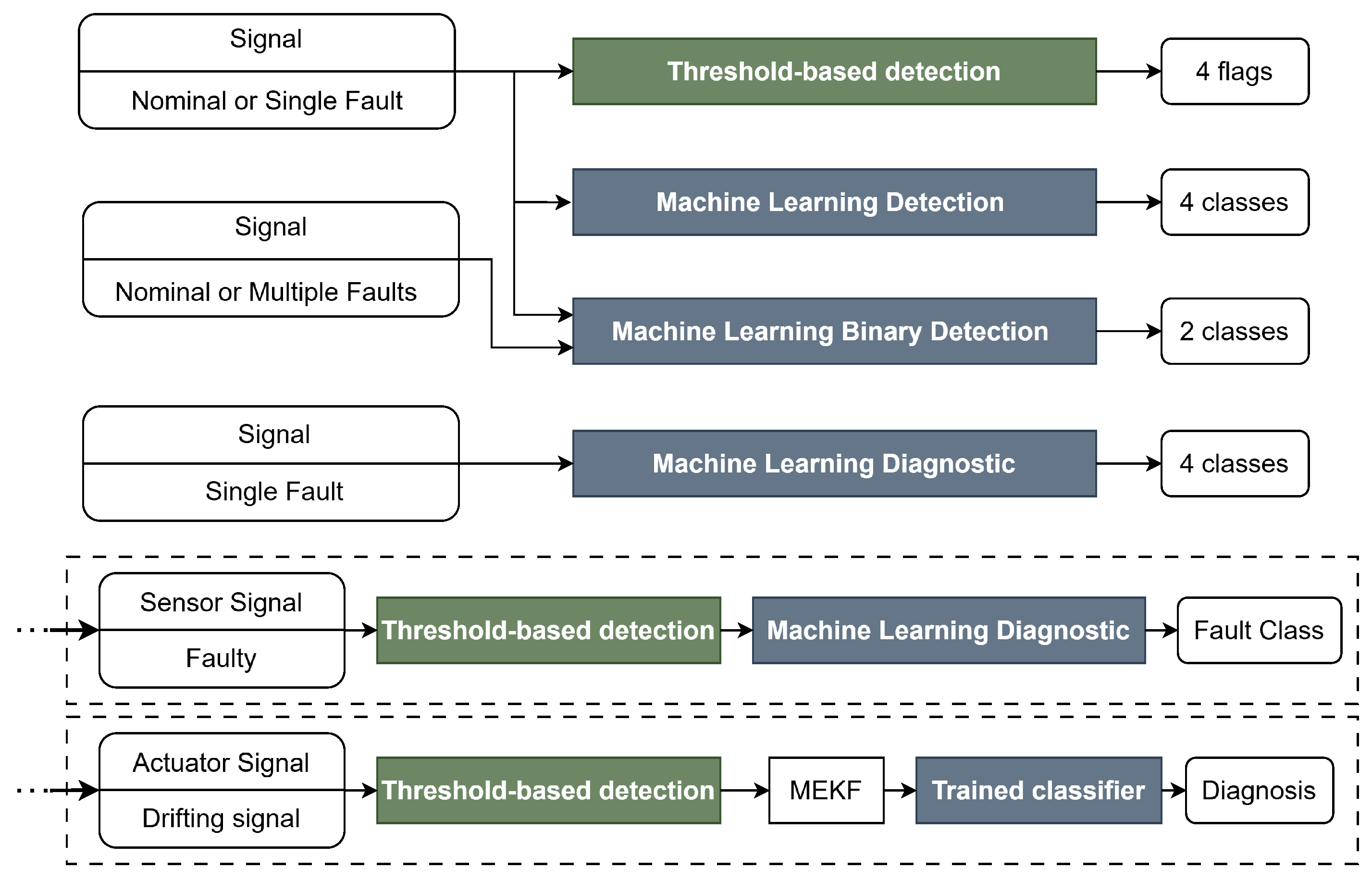
Section 2.1. Trained learning agents in this study are tasked with many different duties, with the number of output classes heavily dependent on the specific task.
Figure 2 shows all the detection methods and the instances in which they are employed: the testing considers first the baseline threshold-based algorithm for a simple detection, and the classifiers for a 4-class classification mimicking a similar behavior. Then, learning agents are tested and specialized on two-class detection, on signals containing one or multiple faults: in addition to that, there is the potential for a real diagnosis, instead of simple detection, which is tested on the same families of classifiers. As final tests, two specific case studies are proposed, where trained classifiers are fully implemented in the functional simulation loop of the satellite, in synergy with the already mentioned variance-based detection algorithm. All of the tests conducted and the results retrieved are reported in
Section 5 in detail.
The data to train the learning agents does not come from an actual mission, but is generated in an acceptably realistic way through the MATLAB
® (R2024b) Simulink
® simulator presented in
Section 4. In the same environment, the proposed classifiers are built and developed through MATLAB
®’s own Classification Learner App: they are various kinds of Support Vector Machines, with the use of different types of kernels and Artificial Neural Networks, following the classic MLP structure, with varying numbers of nodes and layers. All of them are taken among the most basic versions of the respective classifier family and they do not present intricate architectures: this is conducted in order to grant increased repeatability and easiness to implement in other Machine Learning tools and software. Also, they are all Simulink
®-compatible, so that testing is immediate and implementation is simplified. All of the learning agents take a collection of features of the signal as inputs, and give as output the corresponding signal class. The feature pool is also the same for all of the classifiers; therefore, interchangeability is total and performance can be evaluated objectively. The complete list of classifiers used in this study is visible in
Figure 1, and they are once again presented in
Section 5.
2.1. Threshold-Based Detection
The baseline functional simulator already involves a simple fault detection algorithm, which is used as benchmark. This “Classic” algorithm is based on custom-made operators placed after each observed element, with the aim of achieving a simple fault detection. These blocks separate any 3-axis time-variant signal into its three components, then calculate the running variance and running mean on each of the signals, with a moving window of tunable length. The evolving variance of the signal, if checked in real time and coupled with the values of the signal itself, can be an already powerful indicator if some unusual behavior is observed [
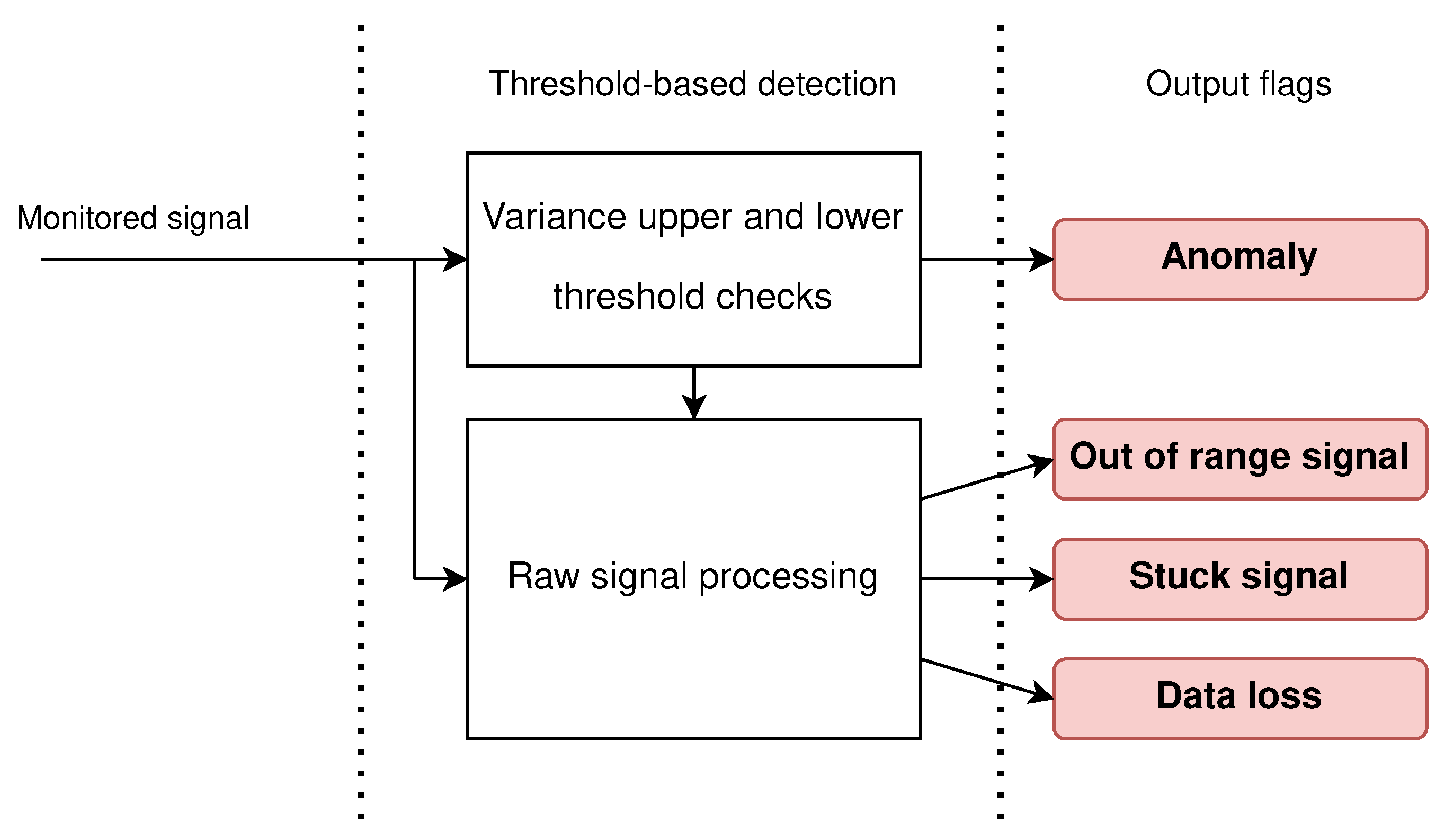
21]. Through a pipeline of logical operators and thresholds, outlined in
Figure 3, this basic algorithm can output four different flags:
Generic anomaly: When any of the axes exhibits a particularly high variance in its signal, a threshold is violated and the block emits a flag.
Out-of-range signal: A simple threshold is put on the maximum magnitude all signals can have, mimicking the violation of the maximum range imposed by physical limits on onboard elements.
Stuck signal: When the block senses a variance drop in the signal to the point where it basically reaches zero, this flag is activated.
Data loss: Just like the previous case, a variance drop is recognized. The detection algorithm goes and checks the effective magnitude of the defective signal as well: if it is exactly zero, then the sensor or actuator monitored is not simply stuck, but it most certainly has stopped outputting meaningful data at all.
Clearly, the generic flag “Anomaly” can be specialized into distinguishing the many faults described in
Section 2.4: this, however, requires a much finer tuning of the detection block and the use of soft thresholding. A finer 6- or 7-class, data-driven, threshold-based detection is most certainly possible, but the tuning would be so specific and custom-tailored on the simulation parameters that it would lose any practical significance and attempt at generality. Some amount of fine-tuning is made nevertheless, to adapt the detector blocks to each of the monitored elements, and re-parametrized on each attitude mode of the satellite: despite the attempts at building an impartial system, given the fine-tuning performed and the fact that also faults are self injected, the correct detection rate is going to be very high. This is also a chance to point out that the necessity to manually and precisely tune so many parameters is one of the weaknesses of this method.
In real detection algorithms, information on the possible behaviors of onboard signals is much more limited, and it is a good idea to keep an intermediate variance threshold: not too high, otherwise it might miss some faulty behaviors, and not too low, to avoid repetitive triggering on false positives. Finally, a delaying function is implemented in each baseline detector, such that any flag recedes back to nominal status only after 10 consecutive samples of no detected faults. This basic data-driven method is a very first benchmark comparison for performances and robustness on Machine Learning classifiers.
2.2. Support Vector Machines
Support Vector Machines are among the most popular learning algorithms, since in terms of relatively small training data, they are efficient and reliable [
12]. The aim of these machines is to build a separator for the data in the form of a hyperplane, with linear equation [
13]
parametrized by vector
and constant
b, to binary classify any entry
. By mapping both the entry data as well as the parameter vector into a higher dimensional space through a transform
, the problem can be moved in a more fit environment for optimized classification, with the separation hyperplane function in the new form [
13]
where a crucial component emerges, the
kernel function:
Few different kernels are adopted in this work, and they are shown in
Section 4.
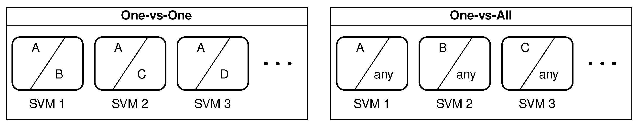
As previously stated, SVMs are binary classifiers, which means that they can potentially distinguish data into one of only two classes. Classification on a number of classes
N higher than 2 is feasible, but only by building many sub-classifiers, as seen in
Figure 4, trained either to distinguish between a class and all others (One-vs-All) or between all possible couplings of classes (One-vs-One). In this research, multi-class classification is approached in a One-vs-One philosophy.
2.3. Neural Networks
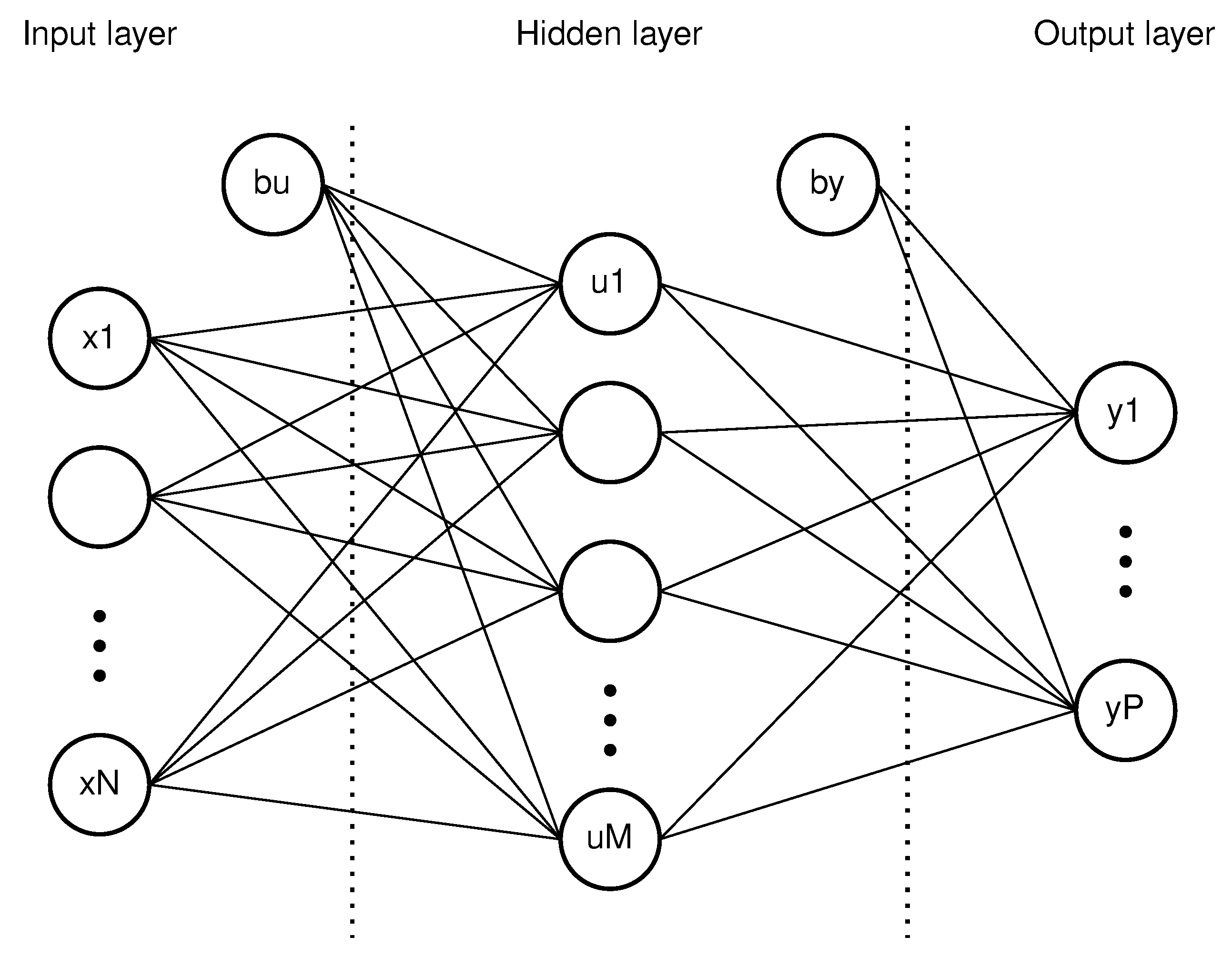
Other widespread classifiers are Artificial Neural Networks, learning agents that improve their accuracy by tuning weights on their internal connections, which for their structure resemble the human brain. In this preliminary analysis, we will focus on one of the most simple layouts: The very popular Multilayer Perceptron (MLP) architecture, portrayed in
Figure 5.
The first immediate “input” layer is defined in its node number
N, by the chosen number of actual inputs of the network, which are the extracted features; the output layer typically contains as many nodes as the total classes
P that the network is able to recognize. Assuming a Fully Connected (FC) architecture, the typical output
of one of the
M nodes in the second (middle) layer is
which is a function of all the
nodes of the previous input layer, of vectors of weights
, and the bias elements
. The activation function is
: in the examined cases of this paper, a rectifier linear unit activation functions (ReLU), equivalent to a ramp function, will be employed from any node to the next one. Then, a normalized exponential function (also known as softmax function) serves as the last activation function for the output layer of the network, in order to produce a probability distribution of the available classes. Some instances of the testing campaign of
Section 5 will employ slightly more complicated architectures, such as Deep Networks with more than one hidden layer, but the current chapter served a basic understanding of the underlying concepts of the most general learning agents.
2.4. Types of Faults on Signals
To understand what kind of inputs the FDIR algorithm has to deal with, it is useful to have an overview of the main kind of trends that could be expected on signals coming from faulty sensors. In practice, there is a limited number of typical behaviors that can summarize most possible faults that a sensor or an actuator could encounter [
1]. A collection of common fault errors is reported in
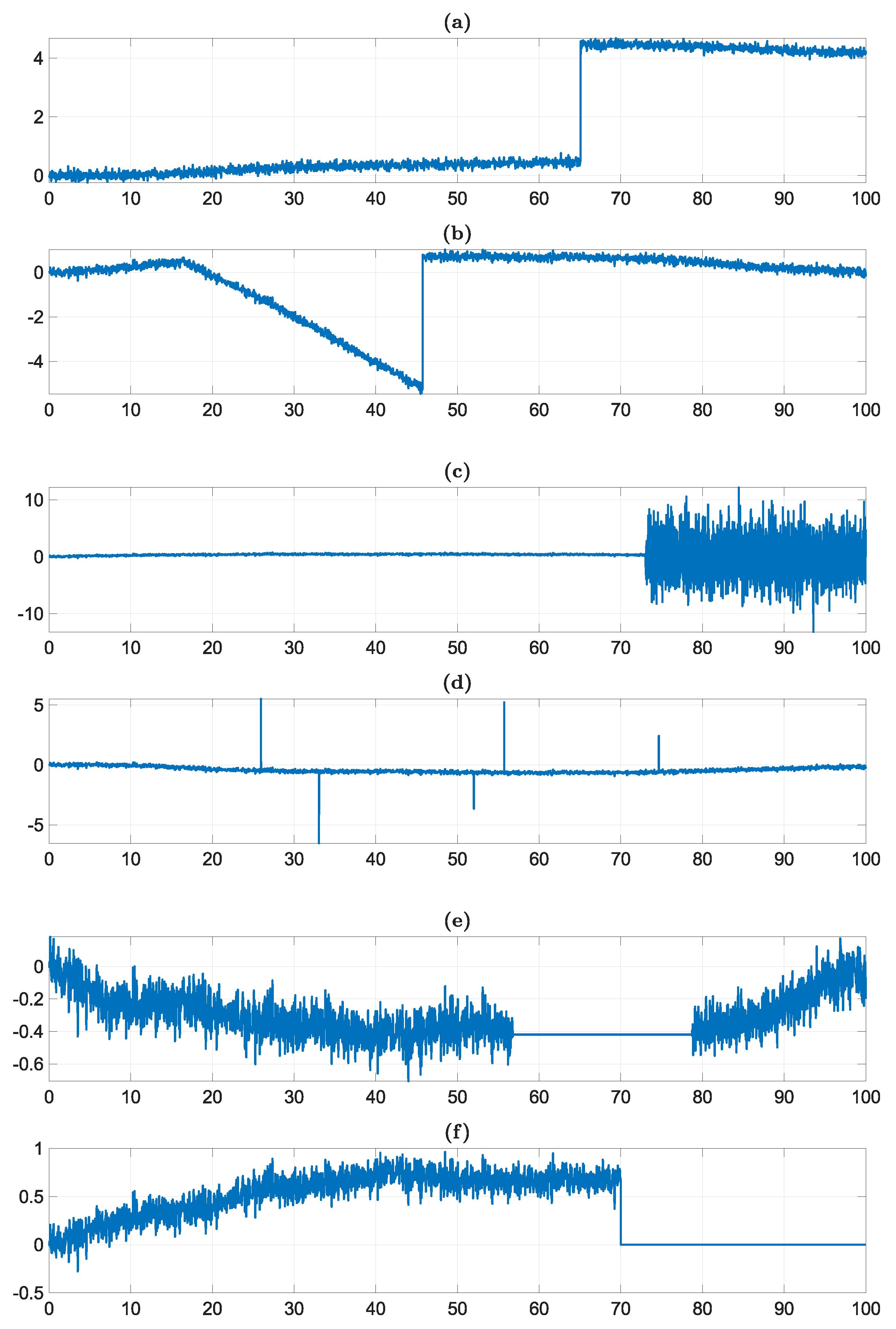
Figure 6, with a brief description for each of them.
Bias: The signal has an abrupt increase or decrease from its normal trend.
Drifting signal fault: The output shows an unexpected linear trend, drifting away from the nominal state.
Erratic behavior: Quality of the signal worsens significantly due to an increase in variance or noise.
Spikes: One or more sudden spikes appear in the output of the signal.
Stuck signal: Signal output gets stuck at a constant value.
Data loss: The signal presents gaps in which no data is available and the output is null.
All of the observed elements in this study, namely the three sensors and the actuator output, are assumed to be possibly subject to any of these faults. Systematic fault injection into nominal signals, for simulation purposes, required fine-tuning to adapt to each of the signals’ orders of magnitude and typical behaviors. If present, faults can appear anywhere between the first and the last of the simulated time, and signals can return to nominality before the end of the simulation, or proceed in their anomalous behavior until the end of the observation. For thorough testing and result collection, the simulation can also apply multiple faults of different types at once on the same signal.
3. Feature Extraction
Datasets are built by running numerous model simulations and therefore collecting nominal and faulty signals, but classification algorithms only receive inputs in the form of a limited number of discrete parameters, which are extracted during the post-processing of data and serve to collect only the most important and characterizing information from any input. This feature extraction phase is the fundamental relationship between the information stored in a raw dataset and the learning abilities of classifiers. The decision on how to choose which parameters to extract is a main topic in the realm of fault diagnosis and signal processing: this research’s contribution is to include parameters coming from different feature extraction philosophies.
Table 1 defines the first batch of time-domain statistical features in the pool.
The first four features include basic and standard statistical quantities, sufficient for what is called simple “novelty detection” on a signal: a change in these features is a very first and macroscopic indicator of a new behavior on the signal, not necessarily a fault [
22]. These features are mean value (AVG), standard deviation (STD), maximum value (MAX), and minimum value (MIN), where standard deviation
is simply the square root of the variance
, which was the main tracked feature for threshold-based detection. The other group of time-related statistical features in the table enhance the overall signal characterization: they are root mean square (RMS), square root of the amplitude (SRA), kurtosis value (KV), skewness value (SV), peak-to-peak value (PPV), crest factor (CF), impulse factor (IF), margin factor (MF), shape factor (SF), and kurtosis factor (KF). These features are well established for capturing behaviors and characterizing time-varying signals [
6,
7], as they are particularly significant: kurtosis, for instance, helps define the amount of extreme values in a distribution, while skewness quantifies the asymmetry of said distribution. Peak-to-peak values, crest factor, impulse factor, and margin factor are signal-based statistical metrics that, especially for relatively regular or periodic signals, are potential markers for outliers. Finally, the shape factor of a signal relates to its shape, while being independent from its magnitude.
Learning entities are provided with some more information concerning the frequency domain, through other typical signal processing features, added to the pool of this work as well [
6]. The signal is further analyzed by extracting the frequency center (FC), root mean square frequency (RMSF), and root variance frequency (RVF), all related to the
N frequency amplitudes
, as shown in
Table 2.
As a last addition to the pool, the feature extraction process calculates the wavelet decomposition of the input 1-D signal using the Daubechies orthogonal wavelet [
6]. This final tool, often used when extracting features from a signal, concerns both the time- and the frequency-domain localization of a signal. By choosing a waveform of reference (in this case, Wavelet Daubechies 4 or “db4”), it is possible to use it as a window function on the signal, while applying different scalings on the wavelet, therefore obtaining a multi-resolution analysis. What is actually saved as additional features to the pool are only the energy percentages corresponding to the approximation (low frequency), and the ones of the details (higher frequencies) up to level 8: by adding these to the previous list, the total number of features in the pool amounts to 26.
Before training a classifier, a feature ranking algorithm is used to associate an importance score to all the predictors fed to the classifier. In the presented work, the chosen ranking is operated by a Minimum Redundancy Maximum Relevance (MRMR) algorithm, which tries to decrease redundancy in the feature pool, while maximizing the relevance of the individual entries of the set.
5. Results
This section deals with the results obtained throughout the work. Initial tests involve comparing the baseline variance-based detection algorithm with classifiers performing a simple four-flag detection. From there onward, the true potential of Machine Learning algorithms is highlighted, starting with a more flexible binary detection, with tests on multiple faults simultaneously and no additional training of the algorithms. Next, innovative techniques are employed on more refined tasks, such as a clear example of fault diagnosis through classification, which is already way out of the capabilities of simple thresholding. Finally, in
Section 5.4 and
Section 5.5, examples of uses in synergy of the two architecture models are explored to point out how a combined use is able to outperform the best capabilities of the individual entities.
The testing campaign involves four kinds of Support Vector Machines, respectively, with linear, quadratic, cubic, and Gaussian kernels: the Gaussian SVM requires a kernel scaling factor of 1.4, while in all instances of multi-class classification, as anticipated, the chosen architecture was One-vs-One. For what concerns Artificial Neural Networks, experiments focused on five different kinds of architectures. First, a small network with only one Fully Connected (FC) layer of 10 nodes; then, a slightly bigger version with 25 nodes in the FC layer; one architecture with a 100-element FC layer; finally, a Bilayered and a Trilayered architecture where each middle FC layer is made of 10 nodes. Activation functions for Neural Networks are always ReLU, except for the last layer, which serves as a probability distribution for the output. The input layer is the same for both SVMs and ANNs, and is made up of the 26 features described in
Section 3. Output layer size changes based on which classification is tested, and all classifiers are summarized in
Table 4.
5.1. Direct Comparison for Simple Detection
A first meaningful test to perform is an exact comparison between classic threshold-based detection and innovative techniques. Since variance-based detection is able to emit three flags plus a simple binary “out-of-range” check, classifiers are trained on a balanced dataset, whose entries exhibit nominal, anomalous, stuck, and loss-of-data behaviors: anomalous behavior can mean any of the faults among bias, erratic, drift, and spikes. Standard threshold-based detection is fed 20 s snippets of signals, as a moving window observing the live evolution of parameters: Machine Learning algorithms are trained on a feature pool extracted by the same dataset, which splices up dataset entries to mimic the same scanning window, as seen in
Figure 9.
By looking at the accuracy results obtained in
Table 5, some considerations can already be made. First off, the consistency of the column dedicated to classic detection, except for one outlier in the last row, reflects how fine-tuning of both faults and the detection thresholds makes it extremely easy to reach high detection rates. The accuracy percentage is not 100% only because classic methods are particularly in trouble when trying to detect drifting signals: if the slope is not steep, variance-based detection is not triggered unless it rapidly comes back to nominal values, therefore generating a spike in the moving variance (see
Figure 6b). However, if the drift does not end before the end of the simulation, and no instrument range is crossed, classic detection might not be triggered at all. In this testing campaign, classic detection is considered successful only if the correct flag is triggered in the first 5 s from the start of a fault: given that faults are programmed to last at least 15% of the time span of the full dataset entry, it is safe to assume that drifts might be almost never detected by variance-based methods. By considering that drifting signals are one of the possible four behaviors labeled under “Anomaly”, and that there are four labels in total, we obtain a probability of a drifting trend happening in any observed signal of
: classic detection misses exactly
to reach complete successful detection of the dataset, which are all instances of drifts. Shifting the focus on classifiers, and by looking at the results mode by mode, some small increase in accuracy can be perceived on those signals whose trend is notoriously smoother (for example, Sun position sensors during a quite steady Earth-pointing mode); apart from that, Gaussian SVMs are reportedly the most unstable and less predictable in terms of behavior.
No particular suggestion on the use of SVMs rather than ANNs can be confidently given: this will come down to ease of implementation, simplicity in design, and computational resources used during their activity, aspects which will be tackled later. The main takeaway from this first batch of tests is that Machine Learning classifiers, when tasked with the same exact duty as the benchmark detection method, reach medium-high accuracy, but are not robust enough to let them deal on their own with this task with no external checks.
5.2. Classifiers for Binary Detection and Multiple Faults
While the baseline threshold-based detection preserves its rigid structure, one of the advantages of learning machines is their flexibility: in the search for an optimal use for classifiers, another strategy is to let them work on a simpler and more general task. For example, the following testing batch in
Table 6 is made on binary classifiers, tasked with the simple acknowledgment of a fault in the object they are monitoring.
This time, the large datasets are equally split between a 50% of perfectly nominal entries, and another 50% of signals that show one of the six basic faults (erratic behavior, drift, spikes, bias, stuck signal, or data loss), with an equal chance of any of them happening to avoid class imbalance. Accuracy results are different with respect to
Table 5, and in some instances, are slightly increased, but still not close enough to a robust and total detection for any sensor or attitude mode in particular. One possible takeaway from this part of the testing campaign could be to use a classifier trained this way in parallel to a classic variance-based detector: this would add redundancy with “competing” software that work on the same task but with two completely different principles and therefore can be a more robust solution with respect to two identical “watchers” working in parallel.
Within binary classification, other experiments can be made. For example, it is possible to study the behavior of classifiers with multiple faults applied. Up until now, all of the considered signals were either nominal or presented only one fault. For this new analysis, a brand new dataset is prepared in this way: half of the signals are completely nominal, the other half present up to two different faults in the same signal. Time segments are prepared in the usual way, which mimics a limited 20 s long moving window, to extract a snippet of signal from a real simulation. The peculiarity of the following analysis is that it is performed with the same binary classifiers tested in
Table 6, which were strictly trained on a dataset containing at most single faults: none of the networks have been re-trained for this second task.
Results for this test are reported in
Table 7: apparently, hyper-parameters in the classifiers and the interpretation of input features were balanced enough to let the machines improve their performances in a lot of instances, despite novel behaviors deviating from what was known from training. It is now clear we are drifting away from classic detection with these cases. While variance-based detection would simply turn on and off in an almost deterministic way due to the extremely specific tuning (while still ignoring drifts), here, the elasticity in behavior and adaptability of the method is much more promising for possible next steps for an enhanced and higher-level detection.
5.3. Targeted Fault Diagnosis and Computational Cost
Classifiers, when charged with similar tasks as classic detection algorithms, are promising, but not optimal. One possible step to take at this point is to exploit the actual “classification” function of Machine Learning agents. Let us imagine an FDIR loop where standard detection is implemented: this basic block can work with thresholds to understand if a signal is stuck or missing, or it can benefit from the binary classifiers tested before to spot any instances where other faulty behaviors are present. Once the “Anomaly” flag is triggered, however, no additional information is given on the type of fault. This first layer of detection has correctly identified a possible error, but has no immediate additional information to transmit to the system or to flight engineers. What the algorithm could do, instead, is to try and figure out on its own the exact kind of fault, to demonstrate its autonomy and to choose the appropriate response, based on the outcome. For this, an actual “Diagnostics” agent should be invoked: we can imagine it as another classifier which, given a faulty signal, precisely identifies which of the pre-defined anomalies it presents (bias, drift, spikes, erratic).
This is exactly the kind of scenario imagined for the next training and testing batch of classifiers, reported here below in
Table 8. Here, the inputs are all known to be faulty signals, and the classifiers are tasked not with detection anymore, but with an identification of the anomaly, pointing out which of the four classes it belongs to. Results on this approach are much more promising, and showcase a more robust use for Machine Learning classifiers.
All agents show an increased accuracy: presumably, the features extracted from signals are more distinct and separate between one fault and the other, with respect to between a faulty and a nominal signal, like the previous instances. Also, the number and kinds of faults influenced this result: instead of six possible faults sharing the same label, like
Table 6 and
Table 7, faults are now distinct and only four, with the two “stationary” faults (data-loss and stuck) removed, as they are rather easily detectable by a simple imposed threshold, without the need to train a classifier to recognize them.
Given the high correct classification rate throughout the algorithms, the particular choice for which classifier to choose comes down to method preferences or availability and computational cost: for this last point, some important parameters on any Simulink
® model are obtainable through Profiler Reports. For example, by running one of the simulations for a slew maneuver, just like the ones that generated many of the training databases above, what we obtain are the times recorded and reported in
Table 9.
Results are not totally unexpected: the first two rows refer to the four-class detection exactly equivalent to the classic variance-based one, the middle ones are binary fault/non-fault detectors, while the last ones are the more sophisticated diagnostic agents showcased in the example of
Table 8. What can be observed is a general increase in processing speed in trained Neural Networks with respect to SVMs, which is good to know, given that for each example, they were built case by case to be completely interchangeable, maintaining the same inputs and outputs. On another note, Gaussian SVMs maintain their unpredictability and low consistency also in terms of computational resources used. Binary detectors take overall less time with respect to four-class classifiers, which is expected due to the lower internal complexity; four-class diagnostic agents are not too far from the first type of simple detectors in terms of computational time. This can be extremely convenient, since they turned out to be the most accurate and they are usually activated only once classic detection has first assessed a fault occurring.
What might be unexpected to notice are the report results in
Table 10, concerning the baseline threshold-based detection, which was present and fully active in the same example simulation of the slew maneuver reported above.
This outcome, however, is easily explained: timing is way higher on the classic detectors portrayed in
Figure 3; also, their Total Time implicitly contains a lot more signal processing, and thresholding operations with a variance signal, compared instant by instant: any of the above classifier was summoned only about a hundred times in 100 simulated seconds, and its task was simply to gather input features and give back a flag by applying already trained weights.
Training times are a slightly different matter with respect to simulation times of the single classifiers. While the latter concern actual performances and are pivotal for the quickness of the algorithms, training times are a one-time-only cost to pay during the implementation process. They were not reported in each instance, due to their non-recurring nature, but most importantly, for their average order of magnitude, which despite their slightly fluctuating values, is consistent and explained here. To be specific, on the hardware employed for this study, consisting in a 12th generation Intel® Core™ i7-1255U, 1700 MHz (10 cores), mounted on a 16 Gb RAM pc, the training times of all algorithms were well below 10 s: SVMs settled at around 2 s each, while Neural Networks required on a rough average 6 s for their training, in all cases. Important outliers are Cubic SVMs and Trilayered networks, which required up to 8 s of training. These results derive once again from choosing very simple architectures for the two classifier families, and confirm once again the quickness of ML approaches when compared to other strategies, such as Deep Learning. It is easy to see how, even with datasets made of hundreds of entries, training times can be considered minimal in an actual SIL or HIL implementation, and even more in real mission planning scenarios, where they are totally negligible. With these considerations, one may have a lesser concern with these aspects, and care much more about real-time performance: all things considered, trained classifiers might be even more attractive as a solution at this point.
5.4. Possible Use in Synergy: Detection and Diagnosis
As previously stated, combining the two detection philosophies explored in this work tends to give the best results overall. The two final rows of
Figure 2 foresee these last case studies, which concern classifiers perfectly embedded and implemented into the functional simulator, instead of being trained and tested in a distinct environment. As a first example of synergy use, it is possible to replicate exactly the scenario described in
Section 5.3. In this simulation, during a slew maneuver, one of the axes of the magnetometer starts behaving unexpectedly. In particular, some erratic behavior starts at
s into the simulation, as shown in
Figure 10a.
This is a particularly troublesome behavior affecting sensors, since the MEKF placed directly down in the pipeline of the spacecraft data processing might filter out the excessive noise, rendering the fault possibly unnoticeable. However, in the functional simulation, the sensor in question is being monitored by standard detection algorithms: the three axes of the magnetometers are being processed live, and an “Anomaly” flag is almost immediately turned on (
Figure 10b). On a spacecraft provided only with a threshold-based algorithm, the detection function would stop here. However, by applying the strategy described in the previous section, it is possible to start an in-depth diagnosis process, operated by a trained classifier, for a more detailed analysis. Therefore, in this example, the Anomaly flag activates a Large Neural Network for fault diagnosis of Magnetometers (specialized in slew maneuvers), precisely the one trained and tested here before, with details and accuracy reported in
Table 8. The network is activated immediately, at
s, and its sliding window starts to process the past 20 s of simulation, sliding the window and refreshing its output once every second. After a first round where the algorithm seems to have found evidence of spikes on the signal, the network stabilizes its diagnosis by consistently reporting an erratic behavior from
s onward. If this information is communicated to other recovery systems onboard, other decision processes could pick the most appropriate response, basing their choice on more than a simple binary fault alarm. This example is built by directly plugging in the simulation one of the trained networks showcased before, proving how the testing process has followed a highly modular approach.
Additionally, a brief initial instance of mislabeling in
Figure 10c is understandable, since the network is trained, as explained in
Section 2.4, only on signals containing faults that start between the first
and the last
of the analyzed window: an improved version of the same network could be fed more extreme cases during training, so that during its operation, its quickness on recognizing faults can improve.
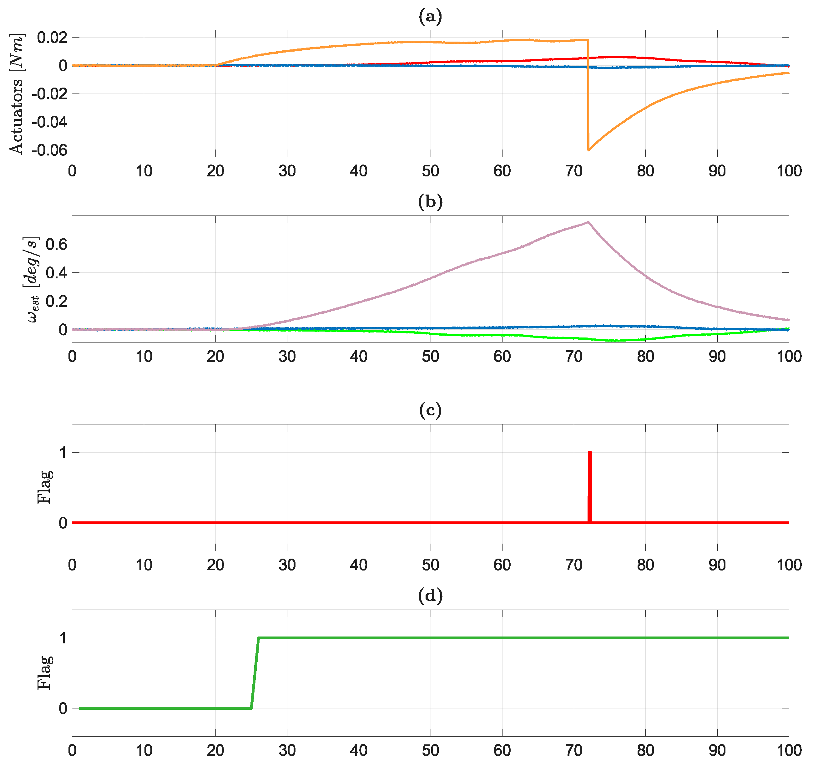
5.5. Possible Use in Synergy: MEKF Enhanced Detection
As a final study case, let us address the main problem found while evaluating threshold-based detection performances: the impossibility to detect drifting signals. A solution could be to set up a learning agent that collects the outputs of the MEKF in the configuration of
Figure 11. The classification network is trained on a dataset of 840 short snippets of MEKF-estimated angular rates, recorded during simulated slew maneuvers, half of which behave in an irregular way due to a drift injected on the actuators. Inputs to the learner are the previously explained 26 features from each one of the axes, so a total of 78 elements. Therefore, once the Neural Network is inserted in the loop, the estimated angular rates incoming from the MEKF need to be split into their three axes components; then, they shall be buffered with the desired length of 20 s at a time, and at that point, features are finally extracted. This is a chance both to show the general setup of a trained learning agent in the loop, as well as to address a more specific and peculiar example: detecting drift faults in actuators, by only looking at MEKF outputs.
Figure 12 explores exactly this case study: the Neural Network detector starts by emitting a null output for the first 20 s, since it does not have enough data to work with. After that, the window starts moving, and real detection effectively starts: it only takes a few seconds, just enough time to incorporate the start of the anomaly in the window, for the network to realize something is wrong and to raise a flag.
It is clear how, despite a lower rate of update of the Neural Network output (the window updates each second, so the resolution is much lower than the sampling time of the simulation), it surpasses the classic threshold-based detector by being extremely quicker and more targeted. As previously said, the training in this case was specifically carried out to identify drifts only, which are the anomalies totally oblivious to classic detection, but it is interesting to notice how the classifier works by monitoring some parameters in a completely different subsystem with respect to the location of the fault. It is easy to imagine other examples of classifiers and classic detection coming together to fill each others’ weaknesses and blind spots, even while staying in the realm of simple detection.
6. Final Remarks
In this research, the challenge of a reliable data-driven fault detection and diagnosis strategy for space systems is explored. The focus has been brought in particular to Support Vector Machines and Neural Networks, trained and validated by large datasets produced in a high-fidelity functional engineering simulator, and compared with a benchmark variance-based method. The kinds of possible faults happening on a space platform can be reduced to a small pool of basic instances, and the feature extraction phase has been showcased in detail as one of the main elements responsible for the quality and accuracy of classifiers in use. After a description of the hypotheses employed and details of the satellite replicated in the simulation, the testing phase was finally set up.
The benchmark classic threshold-based detection algorithm has shown its strength points and weaknesses in terms of the accuracy reached even with a meticulous tuning of parameters. The completely different approach and higher flexibility given by AI-aided classifiers apparently hints to a progressive substitution of classic methods, or at least to a use in parallel of both methods for a fail-safe redundancy. However, performances of classifiers are not robust enough to confidently replace classic methods in their totality: what is recommended instead is a work in synergy, to outperform the capabilities of both the individual architectures. Classic detection is optimal for simple checks, like the ones that signal an out-of-range sensor or an actuator that is stuck on a constant value, but it runs into trouble when tasked with identifying useful information on a signal with a never-before-seen variance trend with respect to nominality. It would be beneficial, at that point, to let a more refined classifier enter the analysis and come in to support these simple monitoring functions, by filling their capability gaps. Classifiers like SVMs and Neural Networks are able to process signals features with an extraordinary sophistication and ANNs, in particular, with an extremely high computational quickness: apart from the training time needed in the project phase, real-time performances are superior in most instances. By coupling the use of variance-based methods adopting simple thresholds, with the accuracy and quickness of trained learning agents for a deeper diagnosis, much more information can be extracted after a fault has happened, and recovery decisions taken autonomously onboard, if shaped on this enriched awareness of all subsystem statuses, will reach autonomy levels never approached until now. Thanks to Machine Learning and artificial intelligence, spacecraft can reach a high level of robust self-diagnostics, not only for GNC and sensor management but by following this novel paradigm for the entire space system, achieving an increased lifetime and an ever-improving self-healing capability.


