1. Introduction
The production of medical consumables is characterized by high variety, small batch sizes, multiple production cycles, and a high degree of customization [
1,
2]. These features present considerable challenges for manufacturing enterprises in workshop scheduling. On one hand, the frequent and small-batch nature of orders fragments production tasks, increasing the complexity of equipment changeovers and production scheduling [
3]. The high level of customization limits the applicability of standardized processes, introducing significant uncertainty into the manufacturing system [
4]. Collectively, these factors reduce production line utilization and elevate the risks of delivery delays and inventory accumulation, forming a critical bottleneck that constrains the operational efficiency of medical consumable manufacturers.
To address the aforementioned challenges, order splitting and reorganization methods have been widely applied in the manufacturing of medical consumables [
5,
6]. Order splitting decomposes large orders into multiple sub-tasks to enhance production flexibility, while order reorganization optimally integrates these sub-tasks to improve resource utilization. However, existing methods still exhibit several limitations. First, most approaches focus on a single optimization objective, either order splitting or reorganization, without considering their synergistic optimization [
7]. Second, current methods rarely incorporate multi-dimensional and multi-scale constraints, such as different product specifications, production batches, and resource matching, which limits their adaptability to complex manufacturing environments [
8].
Therefore, this study proposes a multi-dimensional, multi-scale bi-level collaborative optimization method for order splitting and reorganization in the manufacturing of medical consumables. A bi-level optimization model is developed, in which the upper level optimizes the order splitting strategy, and the lower level optimizes the reorganization of production tasks to ensure efficiency and rationality in the manufacturing process. The model comprehensively accounts for order characteristics, production resource constraints, and delivery requirements, and it is solved using a bi-level multi-objective optimization algorithm to balance production costs and delivery time. The main contributions of this study are as follows:
- (1)
A bi-level collaborative optimization model for order splitting and reorganization is developed to address the limitation in existing studies that treat these processes independently.
- (2)
The model considers the multi-dimensional and multi-scale characteristics of medical consumables, which are often overlooked in prior research, enhancing its adaptability and practical applicability.
- (3)
A bi-level hybrid multi-objective optimization algorithm is proposed to solve the model efficiently, filling the gap in the literature where most optimization methods remain single-layered or single-objective.
The remainder of this paper is organized as follows:
Section 2 presents a literature review, analyzing the current research status and limitations of existing order splitting and reorganization methods.
Section 3 establishes the bi-level optimization model for order splitting and reorganization.
Section 4 presents a bi-level hybrid multi-objective optimization algorithm for solving the model.
Section 5 verifies the effectiveness of the proposed method through a case study. Finally,
Section 6 concludes this study and outlines directions for future research.
2. Literature Review
The splitting and reorganization of order tasks constitute a critical component of order management in medical device manufacturing enterprises. When confronted with order tasks involving complex product specifications, a well-designed splitting and reorganization strategy can significantly enhance production efficiency and resource utilization within workshops, while effectively reducing delivery lead times [
9]. In recent years, research on order splitting and reorganization has primarily focused on the following aspects: order splitting and order reorganization.
Order task splitting refers to the process of breaking down a complex, multi-specification order task into multiple smaller and more manageable manufacturing sub-tasks, thereby facilitating the optimization of production management [
10]. Existing studies are primarily grounded in operations research and systems engineering theories, often integrated with modern information technologies to enable effective order splitting. Some researchers have adopted hierarchical splitting methods [
11], which progressively decompose orders based on complexity and product structure across different levels. These methods are typically suitable for multi-level, multi-stage manufacturing processes. Li et al. [
12], aiming to optimize cost-effectiveness in manufacturing, proposed a task splitting strategy based on cost-controlled optimization and equipment Bills of Materials (BoMs). They abstracted the task splitting and equipment cycle scheduling process into a mathematical model, formulating specific optimization objectives and constraints to identify the optimal splitting strategy. Li et al. [
13] first applied the 5S management methodology to preprocess enterprise production order data. Then, based on a seven-layer progressive model that comprehensively considers time, cost, and service factors, they developed an order splitting model oriented toward data cleansing and transformation, thereby enabling efficient collaborative production among various workshop stations. Ding et al. [
14] designed a splitting-based collaborative method for task planning, establishing a product development process for fine-grained tasks. Targeting the minimization of makespan, they implemented task splitting under fine-grained splitting conditions, aligning with managerial preferences for granular manufacturing tasks. Another splitting approach is known as dynamic splitting. This method dynamically adjusts the task splitting strategy in response to changes in order demand and is commonly used in industries with highly volatile demand, such as fast-moving consumer goods and medical consumables manufacturing. Mateus et al. [
15] proposed a task prioritization model for identifying assembly sequences. Unlike conventional identification methods, this model dynamically adjusts the splitting sequence of various modules by recognizing subassemblies and their respective priorities, as well as the priorities of their parent assemblies.
Order reorganization refers to the process of reordering and optimally recombining the decomposed manufacturing sub-tasks based on the enterprise’s actual production capacity, resource availability, and market demand, with the goal of ensuring continuity and efficiency in production [
16]. Existing reorganization methods generally fall into two categories: capacity-based task reorganization methods and multi-objective optimization-based reorganization approaches. Du et al. [
17], under resource-constrained conditions, proposed a bi-objective manufacturing task reorganization method that integrates hybrid intuitionistic fuzzy information entropy. The model aims to minimize both makespan and energy consumption, and is solved using an improved NSGA-II algorithm. Seyyedabbasi et al. [
18] developed a reinforcement learning-based optimization method for supply chain order reorganization. Designed to address multi-node and multi-level order reorganization problems in supply chains, the approach utilizes the Deep Q-Network (DQN) algorithm to optimize order allocation strategies in real time, thereby enhancing overall supply chain efficiency. Sun et al. [
19] investigated order reorganization strategies in the context of e-commerce, focusing particularly on resource allocation optimization in response to large-scale, sudden order surges. The study proposed a mixed-integer linear programming (MILP) model combined with a dynamic allocation algorithm to reorganize orders in a dynamic environment, significantly improving logistics responsiveness. Gong et al. [
20], addressing the task reorganization game problem in crowdsourcing, proposed a bi-level coordinated optimization model based on a Stackelberg game framework. Aiming to maximize profit at the upper level and minimize cost at the lower level, they developed a nested bi-level genetic algorithm to efficiently solve the reorganization problem.
With the widespread application of artificial intelligence and optimization algorithms, researchers have begun to adopt intelligent optimization techniques such as the genetic algorithm (GA) and Ant Colony Optimization (ACO) to address order splitting problems [
21,
22]. These studies typically start by defining optimization objectives and then constructing optimization models to achieve efficient order splitting, thereby improving resource utilization and reducing production time. Elgendy et al. [
23] proposed a mixed-integer mathematical model and developed a Parallel Distributed Genetic Algorithm (PDGA) to optimize large-scale manufacturing task splitting. The improved PDGA not only increased population diversity but also enhanced the performance and speed of the evolutionary process. Hu et al. [
24] introduced a cloud-based modular task splitting method. This approach innovatively divided the product manufacturing process into four stages—design, production, transportation, and maintenance—to enable modular splitting. Subsequently, a hybrid method based on an improved Artificial Bee Colony (ABC) algorithm was employed to optimize the splitting process. To address the complexity of manufacturing tasks arising from customers’ personalized product demands, Pang et al. [
25] formulated an optimization model with the objective of minimizing makespan. They designed two transition strategies and, by incorporating historical data samples, proposed an improved Whale Optimization Algorithm (WOA) to solve the problem effectively.
To summarize, current research typically treats order splitting and reorganization as separate processes, with limited attention given to the interdependencies between the two, thereby lacking a collaborative optimization perspective. Moreover, most existing studies focus solely on the BoM of products for splitting and reorganization, considering relatively narrow factors. This overlooks multi-scale elements such as production processes and equipment constraints, which are essential for aligning with the practical requirements of enterprise-level manufacturing operations. Therefore, this paper concerns splitting and reorganization based on multi-dimensions and multi-scales.
3. Modeling
3.1. Problem Description
The production model of medical infusion device manufacturers is generally make-to-order (MTO) [
26]. Due to the complexity of product varieties and the limited production resources, traditional order management methods cannot effectively address issues such as order diversity, complex resource constraints, and dynamic changes in order demand [
27]. Therefore, this paper proposes a multi-dimensional and multi-scale bi-level collaborative optimization model for order splitting and reorganization, aiming to develop rational strategies for order splitting and reorganization that improve production efficiency, reduce production costs, and meet order delivery deadlines.
As shown in
Figure 1, the model is divided into two levels. The upper level mainly focuses on the order splitting process, which is responsible for decomposing the order demand plan into multiple orders and product specifications, ultimately breaking down orders into several sub-orders (
Oi denotes the i-th original order,
Sij denotes the
j-th specification within order
Oi,
Tijk refers to the
k-th sub-order derived from specification
Sij). The objective of this splitting process is to achieve an optimal granularity in order splitting. The lower level primarily focuses on the order reorganization process; it takes the set of sub-orders generated by the upper level as input and then reorganizes them into a new set of orders according to the relevant constraints. Its objective is to minimize production costs as well as order delivery delays. Throughout the entire process of order splitting and reorganization, multi-dimensional criteria (i.e., materials, processes, equipment, and labor efficiency) and multi-scale criteria (i.e., finished products, components, subassemblies, and parts) are adhered to, thereby considering various limitations encountered in actual production processes. Moreover, the upper-level order splitting provides input for the lower-level order reorganization, and the reorganization results are fed back to the upper level for adjustments. Through repeated iterative collaborative optimization, the final optimal production orders are achieved.
In constructing the order splitting and reorganization model, and in order to realistically reflect the production processes of the enterprise while simplifying the complexities of real-world situations to render the model feasible and solvable, the following assumptions are made to satisfy the basic conditions of this bi-level collaborative optimization model:
- (1)
All order demand quantities are assumed to be deterministic throughout the order splitting and reorganization optimization process.
- (2)
The material list required for each order is assumed to be fixed, with no substitute materials available.
- (3)
The operations for each order follow a clear sequence, disallowing cross-process manufacturing or the merging of individual processes.
- (4)
Sterilization equipment can be used only once per day and, once assigned to an order task, cannot be interrupted or preempted by another task until the current task is completed.
- (5)
The granularity of order splitting must satisfy a minimum production batch size requirement, and orders cannot be split indefinitely, in order to ensure processing economy.
3.2. Notation Description
To construct the mathematical model, this paper employs a series of symbols, the definitions and descriptions of which are shown in
Table 1.
3.3. Model for Order Splitting Level
In the demand plan for medical infusion device orders, multiple orders are typically involved. Each order generally comprises products with various specifications, and each product consists of multiple parts. The primary purpose of the order splitting level is to decompose the demand plan into several parts orders under certain constraints. The objectives of the order splitting level mainly include achieving optimal splitting granularity and minimizing splitting costs.
- (1)
Splitting granularity. Splitting granularity refers to the production quantity or scale of each sub-order and its distribution when an overall order is divided into multiple sub-orders. A reasonable splitting granularity requires that each sub-order is neither excessively large nor excessively small, which is manifested in three aspects: economic efficiency, flexibility in production scheduling, and coordination and balance. The mathematical expression is as follows:
where
P1,
P2, and
P3 represent the penalty functions for economic efficiency, flexibility in production scheduling, and coordination and balance, respectively, and F denotes the splitting granularity function. The model aims to minimize the splitting granularity penalty.
- (2)
Split costs. The order splitting cost can be regarded as the additional cost incurred during the process of dividing an overall order into multiple parts orders. These costs primarily manifest as equipment preparation and changeover costs, material scheduling and logistics costs, and planning and management costs. Its mathematical expression is shown as follows:
where
Cequ, Cmat, and
Cplan represent equipment changeover costs, material scheduling costs, and planning costs, respectively.
After completing the construction of the splitting granularity and splitting cost models, the objective function of the mathematical model for the order splitting level can be expressed as Equations (7) and (8).
where Equation (7) aims to minimize the splitting granularity and Equation (8) aims to minimize the whole split costs.
Additionally, the constraints are divided into splitting granularity constraints and splitting cost constraints, and the related constraints are expressed by Equations (9)–(22).
where Equations (9)–(15) define the constraints related to splitting granularity. Specifically, Constraint (9) ensures that the production quantity of each part is not less than the economic batch size to avoid excessive costs caused by irrational splits. Constraint (10) limits the total setup cost within the budget. Constraint (11) ensures that equipment workloads do not exceed their capacity. Constraint (12) requires compatibility in sterilization methods among parts within the same order, while Constraint (13) restricts each part type in the same order to a single specification for scheduling consistency. Constraint (14) mandates that the production quantity meets demand while reserving safety stock, with
α as the safety factor. Constraint (15) ensures that the total time for production and distribution does not exceed the delivery deadline of the final product.
Equations (16)–(22) address constraints related to splitting costs. Constraint (16) ensures that the processing time of each sub-task on a given machine does not exceed its actual capacity. Constraint (17) restricts material consumption to the available supply. Constraint (18) links material scheduling and transportation costs to the number and size of sub-tasks. Constraint (19) controls the number of splits per product type to limit excessive planning and management costs. Constraint (20) sets a minimum production batch size for each sub-task. Constraint (21) ensures sub-tasks are completed within the delivery time frame. Finally, Constraint (22) enforces non-negativity and binary decision conditions on the model variables.
3.4. Model for Order Reorganization Level
After being processed by the order splitting level, the demand plan is divided into multiple sub-order tasks, which are then passed to the order reorganization level for further processing. The order reorganization level optimizes the production sequence, process flow, and resource scheduling of each sub-task to ensure efficient task completion while preventing excessive equipment usage, frequent process changes, and material waste. Additionally, by optimizing task prioritization and scheduling, the reorganization level ensures that all sub-tasks are completed on time, reducing extra costs caused by delays. This enhances production efficiency, lowers costs, and guarantees on-time delivery. Therefore, the main objectives of the order reorganization level are twofold: minimizing production costs and minimizing order delivery delays.
- (1)
Production costs. In the process of constructing a mathematical model with the goal of minimizing the production cost of orders after restructuring, it is necessary to comprehensively consider the changes and impacts of material costs, labor costs, and equipment costs during the order restructuring process. The mathematical expression is as follows:
where
C_mat,
C_lab, and
C_mac represent material costs, labor costs, and equipment costs, respectively.
- (2)
Delivery delays. In the order reorganization model, incorporating delayed delivery time as one of the optimization objectives is significant as it systematically balances production resource allocation and order prioritization, effectively reducing order delivery delays. This, in turn, enhances customer satisfaction and strengthens the company’s reputation. Since an order demand plan consists of multiple orders, and each order includes multiple product specifications, the delivery delay time of each order is determined by the latest delivery time among its product specifications. The total delivery delay time is the sum of the delivery delays of all orders. Therefore, the total delivery delay time of an order demand plan can be obtained using Equation (26).
After completing the construction of the production cost and delivery delay models, the objective function of the mathematical model for the order reorganization level can be expressed as Equations (27) and (28).
Meanwhile, throughout the order reorganization process, this study also establishes constraints from multiple dimensions, including materials, processes, equipment, and work efficiency.
Equations (29)–(31) define the material-level constraints, where Equation (29) represents the material inventory constraint, Equation (30) addresses material compatibility, and Equation (31) enforces the minimum material batch size constraint. Equations (32)–(34) specify the process-level constraints, including process sequence constraints (Equation (32)), process parallelism constraints (Equation (33)), and process dependency constraints (Equation (34)). Equations (35)–(38) describe the equipment-level constraints, which cover equipment capacity (Equation (35)), equipment exclusivity (Equation (36)), and equipment changeover time constraints (Equations (37) and (38)). Equations (39) and (40) capture the labor-efficiency-related constraints, including labor efficiency fluctuation (Equation (39)) and worker skill matching (Equation (40)). Finally, Equations (41)–(43) represent other comprehensive constraints, where Equation (41) ensures order integrity, Equation (42) guarantees non-negative delivery delay, and Equation (43) incorporates order priority constraints.
3.5. Bi-Level Collaborative Optimization Model for Order Splitting and Reorganization
After completing the modeling of the order splitting level and the order reorganization level separately, mathematical processing methods are required to integrate both models into a unified framework, enabling a more comprehensive global optimization of the two-stage order splitting-reorganization process. Based on the characteristics of the order splitting and order reorganization models, commonly used mathematical processing methods include constraint transformation, hierarchical weighting, joint multi-objective optimization, and bi-level collaborative optimization [
28,
29,
30]. Considering the advantages of these four approaches, this study ultimately selects the bi-level collaborative optimization method for mathematical modeling.
Finally, after mathematical processing, the bi-level collaborative optimization model is formulated as shown in Equation (44). In the upper-level optimization, it must be ensured that for each generated splitting scheme
x, there exists a feasible solution
y in the lower level, and
y must be a Pareto-optimal solution for the lower-level bi-objective optimization.
4. The Proposed NSGA-II-MOEA/D-CIS Algorithm
To solve the bi-level collaborative optimization model for order splitting and reorganization constructed in the previous section, this section designs an improved hybrid multi-objective optimization algorithm (NSGA-II-MOEA/D-CIS). Its core components include the Non-dominated Sorting Genetic Algorithm II (NSGA-II) [
31], the Multi-Objective Evolutionary Algorithm based on Decomposition (MOEA/D) [
32], and the collaborative iterative strategy (CIS).
4.1. The Framework of the NSGA-II-MOEA/D-CIS Algorithm
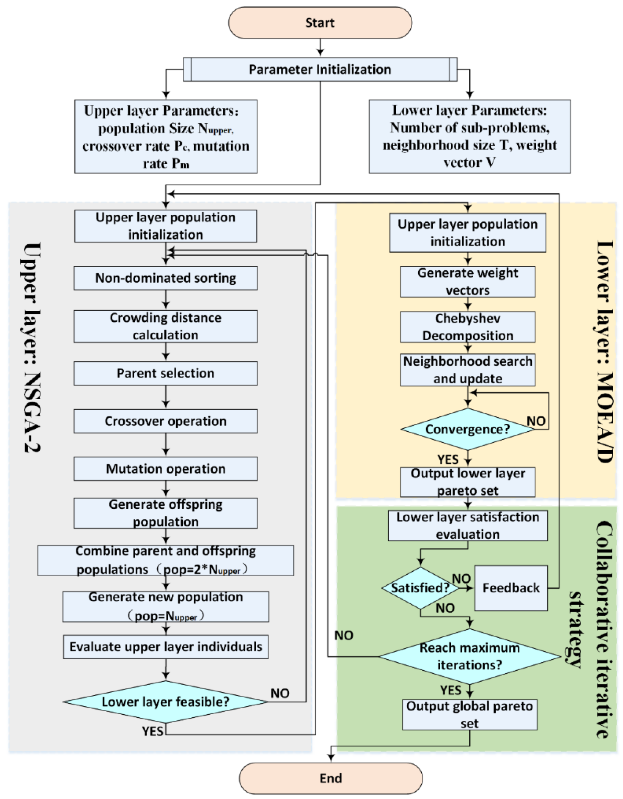
Figure 2 illustrates the process framework of the NSGA-II-MOEA/D-CIS algorithm, with its specific execution steps described as follows:
Step 1: Initialize the algorithm, which includes setting upper-level and lower-level parameters, maximum iteration count, etc. Additionally, the initialization of the upper-level population is performed, generating all chromosomes for the upper-level population.
Step 2: Perform non-dominated sorting on all individuals in the upper-level population based on their fitness values, followed by crowding distance calculation.
Step 3: Apply genetic operators to the upper-level population, including selection, crossover, and mutation, to generate the offspring population.
Step 4: Merge the initial population with the offspring population and generate a new population based on non-dominated sorting and crowding distance calculation.
Step 5: Traverse the upper-level population; if any individual results in an infeasible solution in the lower level, return to Step 2. Specifically, each upper-layer individual represents a particular order splitting scheme. Before being passed to the lower layer, these individuals are evaluated based on structural feasibility, i.e., whether their corresponding order splits can be reassembled into valid production plans.
Step 6: Transfer the upper-level population that meets the requirements to the lower level, initialize the MOEA/D population, and generate weight vectors for each individual.
Step 7: Apply the Chebyshev decomposition method to decompose the bi-objective lower-level model into multiple subproblems. Define the neighborhood for each subproblem and perform neighborhood updates.
Step 8: Solve the lower-level problem iteratively to obtain the Pareto front.
Step 9: Execute the collaborative iteration strategy, where the Pareto front of the lower level is evaluated for satisfaction. Unsatisfactory solutions are fed back to the upper level for parameter adjustments. Once all satisfactory individuals are collected, check if the maximum iteration count has been reached. If so, output the final global Pareto solution set; otherwise, return to Step 2.
4.2. Design of the Upper-Level NSGA-II Algorithm
4.2.1. Encoding and Decoding
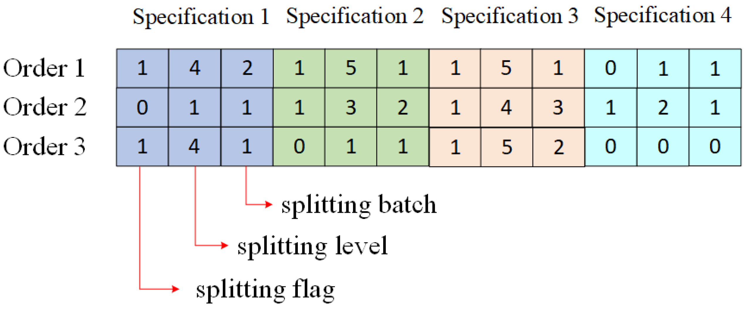
Considering the characteristics of the upper-level order splitting problem and the properties of the NSGA-II algorithm, this section proposes an integer-based matrix encoding method. In this encoding scheme, each chromosome represents an order splitting result, and the chromosome is divided into multiple segments based on the number of product specifications in the order. Each segment of the chromosome includes three key pieces of information: a splitting flag (for quickly distinguishing whether the order has been split), the number of splitting levels (to facilitate the retrieval of sub-orders based on the BoM), and the number of splitting batches (indicating how many batches the order has been split into). The splitting level in this study refers to the recursive depth of order decomposition. A finished product assigned to Level 1 indicates that no further splitting is required. If the order is split once (e.g., into assembly or processing sub-tasks), its components are assigned to Level 2. Further splitting leads to Level 3, and so on. To ensure that all chromosomes have equal lengths, the segments corresponding to missing product specifications are assigned values of 0 for the splitting flag, splitting levels, and splitting batches.
To illustrate the encoding and decoding process of the matrix encoding method more clearly, this paper selects three order splitting instances as examples, where Order 1 contains four product specifications, Order 2 contains four product specifications, and Order 3 contains three product specifications.
Figure 3 presents a numeric matrix that encodes the splitting strategy for multiple orders across different product specifications. Each cell is formatted as batch count/splitting level/splitting flag, representing the production quantity division, hierarchical allocation, and activation status of each specification, respectively.
For example, supposing there are three specifications in Order 3, then all cells of specification 4 are set to 0. In addition, for specification 1, the value 1/4/1 indicates that the specification needs to be split to the fourth level and the quantity divided into a total of one batch. For specification 2, the value 0/1/1 indicates that no split is needed in this specification, so both the splitting level and batch count are set to 1. For specification 3, the value 1/5/2 indicates that the specification needs to be split to the fifth level and the quantity divided into a total of two batches.
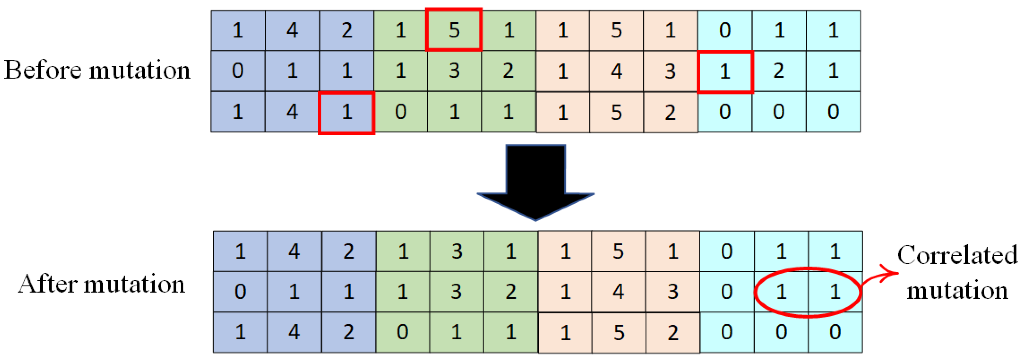
4.2.2. Block Crossover Operator
The purpose of the crossover operation is to exchange genes between parent chromosomes to better explore new regions of the solution space. Since the algorithm adopts an integer matrix encoding scheme, the commonly used simulated binary crossover (SBX) method [
33], which is typically applied to real-valued encoding and generates continuous values, is not well suited for integer matrix encoding. Therefore, this paper adopts a block crossover method tailored to the specific problem. In this approach, during each crossover, the chromosome segments corresponding to a specific product specification are entirely exchanged to preserve the integrity of the decision segment information. The detailed process is illustrated in
Figure 4.
4.2.3. Hierarchical Random Mutation Operator
In the NSGA-II algorithm, the mutation operator introduces “mutations” in one or more genes of a chromosome to increase the probability of escaping local optima and maintaining population diversity. Based on the special encoding rules of the chromosome, this paper adopts a hierarchical random mutation method, where a random gene position in different rows of the matrix is selected for mutation. Notably, due to specific encoding constraints (i.e., if the splitting flag is 0, both the splitting level and batch count are set to 1), when a mutation occurs in the splitting flag gene position, the corresponding splitting level and batch count must also be modified accordingly. The detailed process is illustrated in
Figure 5.
4.3. Design of the Lower-Lever MOEA/D Algorithm
4.3.1. Encoding and Decoding
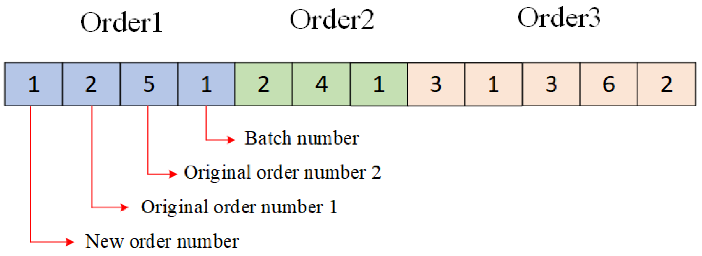
Considering the characteristics of the lower-level order reorganization problem and the properties of the MOEA/D algorithm, this section adopts an integer vector encoding method. In this encoding scheme, the entire chromosome is divided into multiple segments, with each segment representing a newly reorganized order. Each chromosome segment is structured as a variable-length gene block, which includes the first gene (new order number), one or more middle genes (original order number from which the new order is derived), and the last gene (the assigned number of production batches for this new order). To illustrate the encoding and decoding process of this integer vector representation more clearly, this paper selects three order reorganization instances as examples. In these instances, Orders 1, 2, and 3 are reorganized from 2, 1, and 3 original orders, respectively.
Figure 6 presents the encoding result of one feasible solution.
Additionally, the decoded result of this chromosome is as follows: New Order 1 is composed of Original Orders 2 and 5, reorganized into a single batch. New Order 2 is composed of Original Order 4, reorganized into a single batch. New Order 3 is composed of Original Orders 1, 3, and 6, reorganized into two batches.
4.3.2. Generation of Weight Vector
In the MOEA/D algorithm, weight vectors are used to decompose a multi-objective optimization problem into multiple single-objective subproblems [
34]. After decomposition, each subproblem corresponds to a specific weight vector. These weight vectors guide the search direction of the algorithm, and well-designed weight vectors ensure that the solutions are evenly distributed along the Pareto front. Since the lower-level optimization model involves only two objectives, an equal-spaced weight generation method can be used. This method first determines the number of intervals and then generates weight vectors uniformly using the reciprocal of the interval count as the step size [
35]. The mathematical expression is given in Equation (45).
4.3.3. Objective Decomposition
One of the key features of the MOEA/D algorithm is that it aggregates multiple objectives from the original multi-objective problem into several single-objective optimization problems using linear or nonlinear methods. Considering the characteristics of the model, this paper adopts the Chebyshev method for objective aggregation [
36]. This method evaluates the overall performance of a candidate solution by measuring the maximum weighted deviation from the ideal point (typically the best value of each objective function in the current population). The mathematical formulation of this process is given in Equations (46) and (47).
4.3.4. Uniform Crossover and Swap Mutation
To ensure that the MOEA/D algorithm collaboratively optimizes subproblems within the weight vector neighborhood while maintaining global search capability and ultimately obtaining a well-distributed and widely covered multi-objective optimization solution set, crossover and mutation genetic operations are applied in the algorithm. Considering the proposed integer encoding method and encoding rules, this section adopts a uniform crossover operator and a swap mutation operator. The uniform crossover operator first randomly generates a set of masks (binary values of 1 or 0, with a length equal to the total number of genes in a chromosome). Then, two parent chromosomes undergo crossover based on this mask (genes are exchanged where the mask is 1, while they are unchanged where the mask is 0). The swap mutation operator randomly selects two gene positions and swaps their values. The detailed operations of these two operators are illustrated in
Figure 7.
4.4. Design of the Collaborative Iterative Strategy
The core of the collaborative iterative strategy (CIS) is to connect the upper and lower optimization processes through a dynamic feedback mechanism. The optimization results from the lower-level MOEA/D are evaluated for satisfaction. If they do not meet the upper-level requirements, the upper-level NSGA-II parameters are adjusted to regenerate solutions, which are then fed back to the lower level for further optimization. This process continues iteratively until a mutually satisfactory solution is obtained, forming a closed-loop optimization. The specific implementation steps of this collaborative iterative strategy are as follows:
Step 1: Objective normalization. To eliminate the impact of dimensional differences between different objectives on the evaluation results, we first normalize the lower-level objectives—production cost and delayed delivery time—into the same range. After normalization, both optimization objectives will fall within the [0,1] interval. The normalization formula used is as follows:
Step 2: Constructing the satisfaction function. Based on the normalized objectives, a comprehensive satisfaction function S is constructed to reflect the overall quality of the lower-level solutions. A commonly used approach is the weighted sum model, which is mathematically expressed as follows:
where α and β are weight functions that reflect the importance of production cost and delayed delivery time, respectively, with their sum equal to 1.
Step 3: Satisfaction evaluation. For each solution obtained from the lower-level MOEA/D optimization, this paper calculates its satisfaction value S and compares it with a predefined satisfaction threshold. If S is lower than the threshold, the solution is considered unsatisfactory. The satisfaction threshold can be determined based on historical production report data. Specifically, this paper extracts the production cost and delayed delivery time data corresponding to each historical order within a given period. After normalizing and weighting these two factors, the average across all orders is taken to obtain the satisfaction threshold.
Step 4: Feedback and parameter adjustment. If unsatisfactory solutions exist in Step 3, feedback is provided to the upper level, and the parameters are adjusted using the following three methods:
- (1)
Dynamic adjustment of objective weights. If the lower-level delayed delivery time is too high, increase the weight of the splitting granularity objective in the upper level to enforce finer-grained splitting solutions (finer granularity may reduce single-batch load, thus decreasing delayed delivery time). Conversely, if the lower-level production cost is too high, increase the weight of the splitting cost objective in the upper level to generate coarser-grained splitting solutions (coarser granularity may reduce production batches, thereby lowering equipment switching costs).
- (2)
Population injection and elite retention. Select upper-level solutions that lead to better lower-level performance and retain them as elite individuals.
- (3)
Algorithm parameter adjustment. If unsatisfactory solutions persist over multiple iterations, adjust the crossover rate and mutation rate of the upper-level NSGA-II algorithm to prevent prolonged stagnation in local optima.
Step 5: Iterative optimization. Continue executing Steps 1 to 4 until a sufficient number of satisfactory solutions are generated or the maximum number of iterations is reached.
5. Case Study
This section aims to conduct a case study on the real-world order splitting and reorganization optimization problem in medical infusion device manufacturing enterprises (Wuhan, China). Through a series of experiments, it verifies the practicality and reliability of the proposed dual-level collaborative optimization model for order splitting and reorganization, as well as the NSGA-II-MOEA/D-CIS hybrid algorithm introduced in previous chapters. First, a set of order data provided by the enterprise is organized to fully demonstrate the multi-dimensional and multi-scale characteristics of the orders. Second, a series of orthogonal experiments are conducted to determine the algorithm parameters, facilitating subsequent algorithm execution. Then, performance comparison experiments are carried out to compare the proposed NSGA-II-MOEA/D-CIS hybrid algorithm with other commonly used algorithms. Finally, the effectiveness of the proposed collaborative iterative strategy is validated through comparative experiments. The experiments in this section are conducted in the following software and hardware environment: Windows 11 operating system, Matlab R2024a integrated development environment, 12-core 13th-generation 2.6 GHz i5 CPU, 32 GB RAM, and 1 TB SSD.
5.1. Data Source Description
The primary case study data in this section is sourced from a domestic medical infusion device manufacturing enterprise. This company is a high-tech enterprise that integrates multiple supply chain processes, including sales, procurement, and production, and specializes in manufacturing infusion sets, syringes, filters, and other related products.
As shown in
Table 2, for testing purposes, this section selects 15 orders from a continuous time period within the enterprise. Each order contains between 3 and 10 different product specifications, with a total of 46 unique specifications after deduplication. Additionally, each order includes key information such as required quantity and delivery time, exhibiting the characteristics of multi-variety and small-batch production. This dataset serves as the fundamental basis for subsequent order splitting and reorganization.
5.2. Parameter Settings
The proposed NSGA-II-MOEA/D-CIS hybrid algorithm in this paper includes three key parameter groups:
- (1)
NSGA-II algorithm: Population size Nupper, crossover rate Pc, and mutation rate Pm.
- (2)
MOEA/D algorithm: Population size Nlower and neighborhood size T.
- (3)
CIS: Iteration count K and satisfaction weights α, β.
To determine the optimal values for these parameters, this section employs the design of experiments (DOE) method for parameter tuning. Since the tuning process is similar across all parameters, this section only presents the optimization process for the three NSGA-II parameters:
Nupper,
Pc, and
Pm. During the DOE process, each of these three parameters is assigned five different levels, as shown in
Table 3. Specifically, the candidate values for population size, crossover rate, and mutation rate were selected based on commonly used settings in multi-objective evolutionary algorithm studies, as well as empirical tuning to balance solution quality and computational cost.
For each parameter combination, the algorithm performance evaluation process is designed as follows:
Step 1: Execute multiple rounds of experiments. For all parameter combinations to be evaluated, conduct 50 independent experiments. In each experiment, each parameter combination independently performs an optimization calculation, generating a corresponding non-dominated solution set.
Step 2: Construct a reference set. After each round of experiments, globally merge the non-dominated solution sets produced by all parameter combinations in that round. Then, filter out individuals in the merged set that are not dominated by any other solutions, forming the benchmark reference set for that round.
Step 3: Compute the single-round contribution rate. For the non-dominated solution set of a given parameter combination in the current round, count the number of solutions that meet the following two conditions:
- (1)
The solution belongs to the solution set of the current parameter combination.
- (2)
The solution is not dominated by any solution in the benchmark reference set.
Divide this count by the total number of solutions in the benchmark reference set to obtain the solution contribution rate of the parameter combination in the current round.
Step 4: Aggregate data across rounds. Compute the arithmetic mean of the contribution rates obtained by each parameter combination over 50 experiments to generate the final comprehensive performance value of that parameter combination.
Step 5: Performance ranking and evaluation. Compare the final performance values of all parameter combinations. A higher value indicates that a larger proportion of effective non-dominated solutions were generated during optimization, meaning better algorithm performance.
Following the above steps, the orthogonal table L25 (3
5) corresponding to the parameter levels in
Table 3, along with the response values, is shown in
Table 4 [
37]. Specifically,
Table 4 displays the results of a designed orthogonal experiment (L25(3
5)) evaluating different combinations of three key algorithm parameters: population size, crossover rate, and mutation rate.
Additionally, by further processing the data in
Table 4, we calculate the average performance value for each parameter at different levels. Sorting these average performance values allows us to determine which parameter has the greatest impact on the performance of the NSGA-II algorithm.
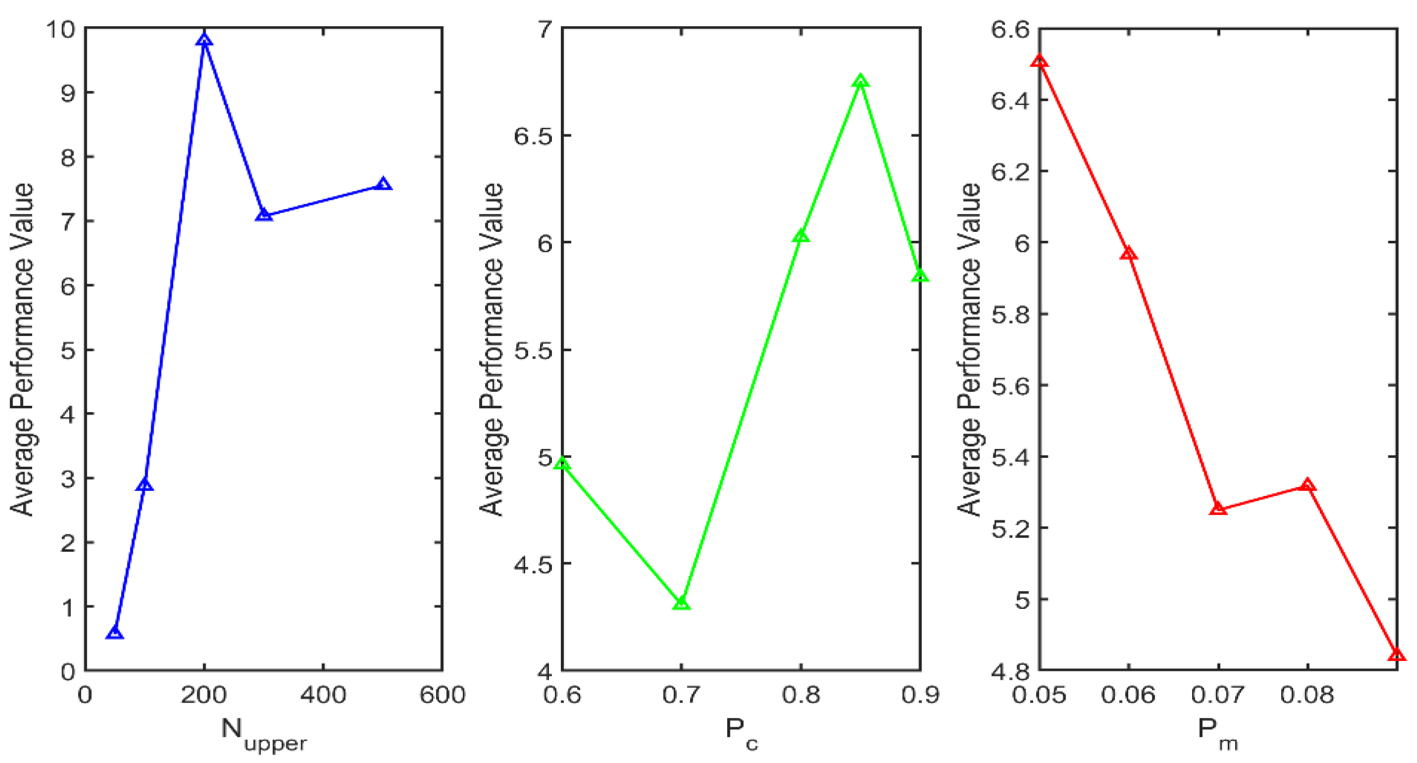
Table 5 summarizes the average performance and range analysis for each parameter level, which supports identifying the most influential parameters. This indicates that among the three parameters, population size has the most significant impact on the performance of the NSGA-II algorithm, and an excessively small population size can negatively affect algorithm performance.
Furthermore,
Figure 8 more clearly illustrates the impact of variations in the three parameters on algorithm performance, based on the calculations in
Table 5. Specifically,
Figure 8 visualizes the relationship between each parameter level and the corresponding average performance, providing an intuitive understanding of how the parameters affect the model outcomes. As shown in
Figure 8, the algorithm achieves the best performance when the population size is set to 200, the crossover probability is set to 0.85, and the mutation probability is set to 0.05. Therefore, this combination is identified as the optimal algorithm parameter setting.
5.3. Comparison Results and Analysis
To validate the advantages of the proposed NSGA-II-MOEA/D-CIS hybrid algorithm in model solving, this case study first combines the upper and lower layers with NSGA-II and MOEA/D algorithms in pairs, resulting in three additional hybrid models: MOEA/D in both the upper and lower layers, NSGA-II in both the upper and lower layers, and MOEA/D in the upper layer with NSGA-II in the lower layer. Additionally, two other multi-objective optimization algorithms are introduced for comparison: Multi-Objective Particle Swarm Optimization (MOPSO) and Strength Pareto Evolutionary Algorithm 2 (SPEA2). MOPSO extends Particle Swarm Optimization (PSO) for multi-objective optimization problems and is widely used in supply chain optimization due to its strong global search capability and rapid convergence. Meanwhile, SPEA2, with its elite archiving mechanism and diversity maintenance, is highly regarded in decision optimization research.
Then, to comprehensively compare the advantages and disadvantages of the hybrid algorithms, this section evaluates them from three dimensions: algorithm performance, model-solving results, and algorithm execution efficiency. To ensure fairness, the parameters of each hybrid algorithm are set according to the parameter configuration method outlined in
Section 5.2, ensuring that all algorithm combinations operate at their optimal performance. Additionally, to address probabilistic variations, each algorithm combination is executed 50 times, and the results are averaged. Furthermore, the collaborative iterative strategy proposed in this paper is applied to all hybrid models.
- (1)
Multi-objective performance comparison. The convergence and distribution of the Pareto solution set are evaluated using indicators such as Hypervolume (HV), Inverted Generational Distance (IGD), Spacing Metric (SP), and Maximum Spread (MS). To facilitate data processing and visualization, all indicator values are normalized to the [0,1] range using min–max normalization. The final comparison results are shown in
Table 6, where ↑ indicates that a larger value within the normal range corresponds to better algorithm performance, while ↓ indicates that a smaller value within the normal range corresponds to better algorithm performance (all subsequent comparison tables follow this notation). Furthermore, each of the four indicators is assigned an equal weight of 25%, resulting in a comprehensive ranking of algorithm performance.
The results indicate that the proposed combination of NSGA-II in the upper layer and MOEA/D in the lower layer achieves the best performance in terms of HV, IGD, and MS metrics, with only a slight disadvantage in the SP metric compared to the NSGA-II-based dual-layer combination. According to the evaluation criteria, the proposed NSGA-II-MOEA/D-CIS algorithm ranks first in overall performance, demonstrating its superiority in solving the optimization problem.
- (2)
Comparison of model solution results. The performance of each algorithm is evaluated based on the obtained Pareto front (only the results of the lower-layer order reorganization are presented). The comparison considers dominance relationships and the number of non-dominated solutions to assess algorithmic effectiveness.
Figure 9 illustrates the Pareto fronts obtained by different algorithmic combinations. The results indicate that NSGA-II-MOEA/D-CIS achieves a superior Pareto front in optimizing both production costs and delayed delivery time compared to other algorithms. Additionally, the number of Pareto solutions obtained by NSGA-II-MOEA/D-CIS is tied for first place (equivalent to the NSGA-II-NSGA-II combination). Furthermore, the findings reveal that NSGA-II exhibits a stronger global search capability than MOEA/D (as evidenced by NSGA-II-NSGA-II ranking second and MOEA/D-MOEA/D ranking sixth). Therefore, incorporating NSGA-II within the hybrid framework significantly enhances the model’s solution quality.
- (3)
Comparison of algorithmic efficiency. The efficiency of each algorithmic combination is evaluated based on convergence generations, execution time, and memory consumption. These factors directly impact the feasibility of solving large-scale problems and the practical applicability of the algorithms. The comparative results are presented in
Table 7. The analysis reveals a dichotomy in the efficiency of homogeneous algorithmic combinations. The MOEA/D-MOEA/D configuration demonstrates superior efficiency due to the natural compatibility of its decomposition strategy, significantly reducing computational redundancy and achieving optimal convergence generations and execution time. This highlights the advantage of algorithmic consistency in strongly coupled multi-objective optimization scenarios. In contrast, the NSGA-II-NSGA-II configuration suffers from the cumulative computational burden of dual-layer non-dominated sorting and crowding distance calculations, leading to high memory consumption and prolonged convergence time. This exposes the limitations of algorithmic consistency in high-complexity problem settings. Furthermore, a deeper analysis of combination patterns reveals that the upper-layer algorithm’s global search capability and the lower-layer algorithm’s constraint-handling efficiency collectively determine the performance ceiling. For instance, MOPSO-MOEA/D leverages the upper-layer MOPSO’s swarm intelligence for rapid exploration of the solution space, while the lower-layer MOEA/D efficiently decomposes subproblems, striking a balance between computational speed and solution stability.
After conducting a comparative analysis of each algorithm across three dimensions—algorithm performance, solution quality, and computational efficiency—a comprehensive ranking was synthesized, yielding the integrated ranking results presented in
Table 8 (with equal weights assigned to each dimension). The results clearly demonstrate that the proposed NSGA-II-MOEA/D-CIS algorithm achieves the highest overall ranking, thereby conclusively validating its applicability in solving bi-level optimization problems.
5.4. Effectiveness Analysis of the Collaborative Iterative Strategy
This section aims to verify whether the collaborative iterative strategy effectively improves the NSGA-II-MOEA/D hybrid algorithm and to what extent. To ensure fairness, both algorithms share identical parameters except for the application of the collaborative iterative strategy. Each algorithm runs 50 times, and the best result is selected.
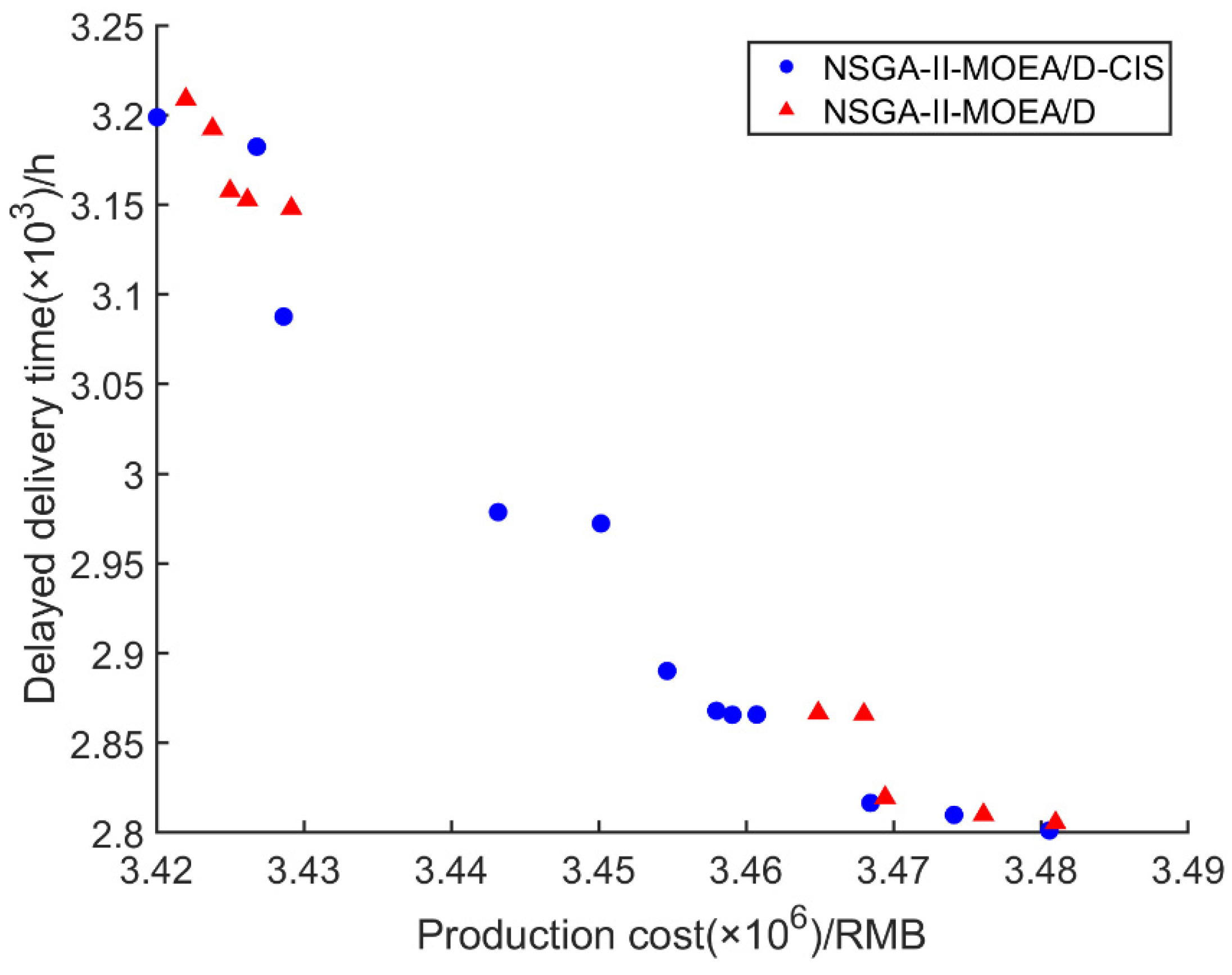
Figure 10 presents the Pareto front comparison between the NSGA-II-MOEA/D-CIS algorithm with the collaborative iterative strategy and the NSGA-II-MOEA/D algorithm without it. As shown in
Figure 10, the Pareto front of NSGA-II-MOEA/D-CIS is broader and exhibits a more evenly distributed solution space. In contrast, the Pareto front of NSGA-II-MOEA/D is more concentrated, either in the region of low production cost with high delayed delivery time or in the region of high production cost with low delayed delivery time. Additionally, NSGA-II-MOEA/D-CIS obtained 12 non-dominated solutions, whereas NSGA-II-MOEA/D obtained only 10. These findings demonstrate that the collaborative iterative strategy effectively expands the solution space and enhances solution diversity.
Moreover, the proposed collaborative iterative strategy is essentially designed to accelerate the convergence process of the algorithm and obtain higher-quality solutions. Therefore, it is necessary to compare the HV indicator (evaluating the uniformity of the solution set) and the IGD indicator (evaluating the proximity of the solution set) for both algorithms.
Figure 11 presents the comparison of the HV and IGD variation curves with and without the collaborative iterative strategy. It can be observed that the NSGA-II-MOEA/D-CIS algorithm reaches convergence at approximately 100 generations, whereas the NSGA-II-MOEA/D algorithm takes around 120 generations to complete convergence, with lower final convergence values than NSGA-II-MOEA/D-CIS. Thus, it can be demonstrated that the collaborative iterative strategy effectively improves the uniformity and proximity of the solution set.
5.5. Scalability Analysis of the Proposed Model and Algorithm
To rigorously evaluate the scalability and computational efficiency of the proposed model under larger problem sizes, this paper conducted extensive simulations using synthetically generated datasets for 30, 60, and 100 orders. These datasets were designed to reflect plausible operational scenarios while focusing on stress-testing the model’s performance under increased scale. The evaluation focuses on four indicators: final Pareto set size, average cost per order, average generations to convergence, and average runtime. The results are summarized in
Table 9 and visually depicted in
Figure 12.
As shown in
Table 9 and
Figure 12, with the number of orders increasing, the size of the final Pareto set grows steadily from 12 to 37, indicating that the algorithm maintains strong diversity and continues to discover a wide range of non-dominated solutions in more complex problem spaces. This suggests good scalability in terms of solution richness. Meanwhile, the average cost per order shows a slight but consistent downward trend from 1.695 to 1.671. This aligns with the expected economies of scale, where larger production volumes allow better resource utilization and cost allocation, thereby reducing unit costs. In addition, the average number of generations required for convergence increases from 84 to 188, which is reasonable as larger-scale problems introduce more decision variables and a broader search space. Similarly, the average runtime increases from 1178 s (15 orders) to 9775 s (100 orders), reflecting the added computational effort required to solve higher-dimensional problems. Nevertheless, the growth remains within acceptable bounds for offline optimization in industrial applications.
In summary, the proposed model and algorithm demonstrate strong scalability, capable of handling increased order complexity while maintaining solution quality, diversity, and computational feasibility.
6. Conclusions and Future Research
To address the challenges of enterprise order scheduling in multi-variety customization environments, this study proposes a bi-level collaborative optimization approach based on multi-dimensional and multi-scale order reconstruction. The proposed framework consists of two core components: an order decomposition level and an order recombination level. The decomposition level optimizes splitting costs and decomposition granularity, and then transmits the results to the recombination layer. Upon receiving the decomposed data, the recombination level generates final regrouping schemes with the dual objectives of minimizing production costs and reducing delivery delays. To solve this bi-level optimization model, a composite bi-layer multi-objective evolutionary algorithm incorporating collaborative iteration strategies is developed. Experimental validation through comparative case studies demonstrates the effectiveness of the algorithm in addressing this class of optimization problems, particularly its superior performance in balancing solution quality and computational efficiency compared to conventional methods. The proposed bi-level collaborative optimization model has strong potential for application in real-world manufacturing settings. In particular, it can be applied to small- and medium-sized enterprises in the medical consumables industry to support intelligent decision making for order splitting, task reorganization, and resource allocation.
In the order splitting and reorganization model, this study considers various factors involved in the order reconstruction process from multiple dimensions (e.g., materials, processes, equipment, and work efficiency) and multiple scales (e.g., finished products, components, subassemblies, and parts). However, while the proposed model demonstrates strong performance in structured and controlled scenarios, certain limitations should be noted. First, the current model assumes deterministic demand, processing times, and capacities, which may not fully capture real-world uncertainty. Second, although the model is designed to be scalable, its computational complexity may become challenging in large-scale industrial applications. Therefore, future research could incorporate uncertainties in demand and resources into the modeling process and employ fuzzy theory to handle and optimize problems characterized by vague or imprecise boundaries.


