Abstract
The reliable operation of rotating machinery is critical in industrial production, necessitating advanced fault diagnosis and maintenance strategies to ensure operational availability. This study employs supervised machine learning algorithms to apply multi-label classification for fault detection in rotating machinery, utilizing a real dataset from multi-sensor systems installed on a suction fan in a typical manufacturing industry. The presented system focuses on multi-modal data analysis, such as vibration analysis, temperature monitoring, and ultrasound, for more effective fault diagnosis. The performance of general machine learning algorithms such as kNN, SVM, RF, and some boosting techniques was evaluated, and it was shown that the Random Forest achieved the best classification accuracy. Feature importance analysis has revealed how specific domain characteristics, such as vibration velocity and ultrasound levels, contribute significantly to performance and enabled the detection of multiple faults simultaneously. The results demonstrate the machine learning model’s ability to retrieve valuable information from multi-sensor data integration, improving predictive maintenance strategies. The presented study contributes a practical framework in intelligent fault diagnosis as it presents an example of a real-world implementation while enabling future improvements in industrial condition-based maintenance systems.
1. Introduction
Industrial rotating machinery is the engine that powers economies through continuous production. Therefore, they must be reliable and efficient to operate without unexpected failures, especially in manufacturing industries. Their failure would lead to costly, unscheduled downtime as well as safety and productivity losses [1,2]. For these reasons, effective maintenance strategies are essential.
Maintenance approaches are categorized into three parts: reactive, preventive, and predictive maintenance [2,3,4]. Among these, predictive maintenance (PdM) has gained popularity due to its ability to predict and prevent failures before they occur. Real-time sensors and monitoring systems can assess the rotating machinery’s health and minimize unplanned downtime, production loss, and associated costs. It is also possible to apply advanced technologies, such as IoT devices and machine learning-based early warning systems, to deliver practical monitoring insights. As a result, PdM has become an integral part of modern industrial systems.
PdM utilizes several diagnostic techniques, among which vibration analysis, temperature monitoring, and ultrasound are the most widely used methods [5,6,7,8,9]. Vibration monitoring is used to identify mechanical faults such as misalignment, imbalance, and gear and bearing defects [1,10,11]. Temperature monitoring is used to observe whether there are overheating issues and/or inefficient lubrication [12,13,14]. Ultrasound can detect early-stage wear and structural defects in bearings and gears that would otherwise be detected later by vibration analysis [5]. Although each parameter provides insight into the working conditions of the rotating parts, integrating them into multi-modal data is still a significant challenge, especially when dealing with complex datasets [15,16].
Fault diagnosis through ultrasound and vibration analysis helps to understand the health status of industrial machines [1,2]. Historically, the relationship between data monitoring and the health status of machines has been observed by engineers’ fault diagnosis skills based on field experience. For example, motor faults can be diagnosed through sounds, while vibration signals collected by portable devices have been manually analyzed to locate bearing faults [17]. However, automating this process would not only shorten the maintenance cycle but could also increase diagnostic accuracy. In this context, a special term has been attributed to the application of machine learning methods in machine fault diagnosis: intelligent fault diagnosis (IFD) [18,19]. This approach proposes machine learning algorithms to train diagnostic tools using the data collected from machines, rather than providing a diagnosis based on the knowledge of maintenance engineers.
Applying machine learning to improve fault classification for the detection and diagnosis of machine faults has been the focus of academic research since the 1990s, and studies in this area have gained momentum since 2015 [17]. Intelligent fault diagnosis expands the capabilities of engineers limited by traditional methods, providing a faster, more accurate, and data-driven diagnostic process. This approach reduces human-induced errors in fault detection and enhances the efficiency of industrial machinery.
Processing data from multiple sensors enables machine learning models to provide conclusive evidence for known failures and generate more accurate predictions. However, integrating multi-sensor data poses unique challenges [20,21]. Fault diagnosis is typically performed on machine components designed to reduce friction and ease rotational movement, such as bearings [9,22], stators [23], gears [24,25], rotors [26], shafts [27,28], and others [29].
This study is motivated by the need to fill the gaps in the existing literature, particularly the limited exploration of multi-modal data integration for fault classification in rotating machinery [30]. These machines are valuable testbeds to study predictive maintenance techniques and are hereby utilized to develop a robust machine learning-based classifier that leverages multi-sensor data fusion for fault detection and classification.
One of the challenges of IFD is the lack of a real-world dataset collected under industrial working conditions. Most studies are based on datasets generated under laboratory conditions [31,32,33,34,35]. However, such datasets often exclude or lack factors such as environmental and operational variables. In fact, these factors can significantly affect machine performance indicators and therefore need to be considered [29] for a robust condition monitoring regime. Datasets that reflect real-world conditions are critical for developing more reliable and generalizable models sensitive to environmental and operational changes. In this context, one of the highlights of this study is that it provides a new dataset collected under real-world conditions. The machine subject analyzed here had a known developing issue of an imbalance in the rotor—which was also verified by examining the data collected via industrial portable analyzers producing a dominant frequency component in the velocity spectrum at exactly the rotation frequency in both the horizontal and vertical directions—generating an extra load due to centrifugal force on the bearings [2]. Such a mechanical fault resulted in an excessive level of velocity amplitudes (mm/s) in the horizontal and vertical axes due to the mismatch of the center of mass and the axis of rotation and a high level of ultrasound due to the increased level of angular contact affecting a relatively smaller diameter (load zone) in the bearing races [36]. As such, this dataset will contribute to research in the field of IFD, allowing a better understanding of the effects of environmental and operational variables.
This study focuses on the following topics:
- Introducing a novel framework for integrating and analyzing multi-modal sensor data for fault diagnosis.
- Benchmarking machine learning classifiers to identify the most effective methods for fault classification.
- Providing insight into the practical implementation of such methodologies in industrial applications.
- Studying possible performance issues related to the quality of raw data, indexes derived from raw data, and identifying the need for additional parameters, both in the time and frequency domains.
- Another, and perhaps the most important, contribution of this study is that it allows for the development of more reliable and generalizable models using a new dataset collected under real-world conditions.
The structure of this article is organized as follows: In Section 2, previous studies are presented in a review of the literature. In Section 3, the theoretical background and machine learning algorithms used in this study are discussed in detail. Comprehensive information on data collection methods, preparation stages, dataset characteristics, and the experimental environment is presented in Section 3.2. In Section 4, the analysis results are discussed, and the performance of the models is compared and analyzed. Finally, in Section 5, the findings and conclusions are summarized, and in Section 6, the study is concluded by including limitations and suggestions for future research.
2. Related Works
In recent years, machine learning and signal processing techniques have made significant advances in fault detection and predictive maintenance in rotating machines. The increasing availability of real and synthetic datasets has offered researchers the opportunity to develop various algorithms in areas such as early fault diagnosis, system monitoring, and maintenance planning and test them on different datasets. This section focuses on current studies on motor and bearing fault detection using vibration analysis, signal processing methods, and machine learning-based approaches. The reviewed literature presents significant developments in the field by addressing the effectiveness and limitations of existing approaches within the framework of the methods used, the nature of the data, and the findings obtained.
Romanssini et al. [3] provided a comprehensive review of vibration monitoring techniques widely used for the predictive maintenance of rotating machinery. They emphasized the importance of vibration measurement as a non-invasive method to diagnose faults in rotating machine components, crucial in preventing unexpected maintenance stops and reducing overall operational costs in heavy industries. The conclusion was that selecting the appropriate vibration monitoring technique is crucial for effective assessments, and the integration of IoT devices could enable real-time monitoring to automatically diagnose mechanical faults.
Pinheiro et al. [5] explored the use of Support Vector Machines (SVMs) to classify rotational unbalanced faults in rotary machines. They used vibration analysis data from an experimental setup using a rigid-shaft rotor. Their study demonstrated that the SVM is effective in classifying faults that are related to the balance of the machine’s axis.
It is hard to identify problems in rolling element bearings, especially when there are strong interfering signals from other machine components such as gears. Randall and Antoni [37] explained how bearing signals have a cyclostationary behavior and used the spectral kurtosis technique to identify the frequency bands where signs of faults are most obvious. Since rolling element-bearing signals are stochastic, they can be separated from deterministic signals, such as those from gears. They coined the term pseudo-cyclostationary to model such signals and observed that discrete/random separation (DRS) is the most efficient technique for separation. DRS works by removing discrete frequency noise from signals. Later, spectral kurtosis is used to describe the identity of the frequency bands where the impulsivity is most pronounced.
Rai and Upadhyay [38] reviewed different signal processing techniques used to detect faults in rolling element bearings. They segmented these techniques into historical stages and highlighted recent advancements that enhanced the diagnostic capabilities. They categorized signal processing methods into three stages based on their historical development: Stage I (pre–2001), Stage II (2001–2010), and Stage III (2011–present). They conclude that selecting the correct signal processing technique is crucial for fault classification accuracy.
Ozkat [39] proposed a machine learning-based methodology to estimate the remaining service life of bearings. Feature extraction, data processing, dimension reduction, and merging steps were applied to calculate the machine’s health indicator from vibration data. Vibration data collected in the time domain was converted to the frequency domain with the Welch method, and feature extraction was performed with traditional statistical indicators.
Pan et al. [9] proposed an improved bearing fault diagnosis method that combines a convolutional neural network (CNN) and a long short-term memory (LSTM) network by processing raw signal data without using any pre-processing or traditional feature extraction steps. While the CNN automatically extracted features from high-dimensional data, LSTM allowed for more effective identification of fault types by considering time dependencies. In their study, they demonstrated that the proposed method achieved over 99% accuracy on the test dataset and that this method outperformed other algorithms for bearing fault diagnosis.
Huynh et al. [7] investigated the use of machine learning techniques, specifically SVMs, to detect ten different failure states in rotating machinery using publicly available datasets obtained from a tachometer, two accelerometers, and a microphone. A total of fifty-eight features were extracted from the time and frequency domains using the short-time Fourier transform, with a window size of 1000 samples and 50% overlap. They achieved a failure classification accuracy of 99.8% using all 58 features with the SVM model. They also aimed to reduce the dimensionality by sorting the features with a decision tree model to rank the important predictors, allowing for the selection of eleven key features. They demonstrated that their approach reduced the training complexity while maintaining a high classification accuracy of 99.7%, achieved in less than half of the training time.
Shandhoosh et al. [40] investigated the performance of different classifiers using statistical, histogram, and ARMA features extracted from vibration data using machine learning techniques for early fault diagnosis in dry friction clutch systems. In the evaluations made with classifiers such as the SVM, k-Nearest Neighbor (kNN), and multilayer perceptron (MLP), the highest accuracy was achieved with methods such as the Random Forest (RF) and kNN. Ensembles consisting of three classifiers combined with the voting strategy achieved higher accuracy rates than the classifiers alone. As a result of the studies conducted, they revealed that the correct feature selection and classifier combination are important in fault identification.
Neupaneve et al. [41] used semi-supervised anomaly detection (AD) techniques to overcome the limitations of supervised learning methods due to the lack of labeled fault data. The study compared the effectiveness of the AD method between traditional techniques and deep learning-based methods and revealed that traditional methods exhibited similar or sometimes superior performance when compared to deep learning techniques. The results obtained indicated that the simplicity and low computational requirements of traditional methods provide advantages and suggested that future research should start with traditional approaches.
Table 1 presents a comparative summary of selected studies on motor fault detection, highlighting the use of both real and synthetic datasets. These works differ in terms of data sources, fault types, and applied methods.

Table 1.
Summary of studies on motor fault detection using real and synthetic datasets.
3. Materials and Methods
3.1. Background
The first approach for a given problem with multiple related parameters is to create a model to solve it. However, the problem might arise with a high level of complexity to formulate a model for several reasons: the problem might inherit non-linearly correlated parameters, or there has not been enough research or attempts to produce reliable models to experiment on. However, if there is information-rich observation data, machine learning algorithms can be used to create models with little or no human intervention [45].
Machine learning can be classified into three categories: supervised learning, unsupervised learning, and reinforcement learning. Unsupervised learning does not operate on labeled datasets but identifies hidden patterns in the data by optimizing a measure of merit [36,46,47]. Reinforcement learning trains models to make sequential decisions by rewarding them through trial and error. Supervised learning is based on training models on labeled datasets and making predictions based on input training data [48]. Input data may be numeric, categorical, textual, etc., and the output data are either continuous values (regression) or a class label (classification).
A classification task involves separating the data into two datasets: a training set and a test set. Each data point in the training set contains several attributes and a target value (label). The goal is to build a model that can predict the target value of the given data with the attributes the model is trained on. The success of the classifier is quantified by validating the test data and presenting it using the performance metrics.
To determine which classification method to use, the best way is to follow a trial-and-error approach [49]. Algorithms such as decision trees, Support Vector Machines, and neural networks are commonly used in supervised learning tasks. Within these methods, the RF, SVM, and boosted DTs are reported as classifiers with relatively higher accuracies [50]. Ensemble methods can also improve model performance by combining multiple weak learners to create a more robust and predictive system [25]. It should also be stated that the effectiveness of supervised learning models is highly dependent on the quality and quantity of the dataset. Insufficient or biased datasets can lead to overfitting or underfitting. To overcome this, methods such as cross-validation and feature selection can be utilized to improve model reliability.
The presented study evaluates the performance of the following machine learning algorithms for fault detection and classification: the SVM, kNN, RF, decision trees (DTs), and several boosting algorithms (XGBoost, Gradient Boosting, AdaBoost, CatBoost, and LightGBM). Due to the large number of classifiers, the following section will define the top performers.
3.1.1. Support Vector Machines (SVMs)
An SVM is a supervised learning algorithm that is used for both classification and regression [51]. It aims to find the optimal hyperplane that separates data points of different classes in the feature space. If the dataset is linearly separable, the SVM aims to maximize the margin between the closest points of support vectors. However, for non-linearly separable data, it is possible to use different kernels (linear, polynomial, radial basis function, etc.) for projecting the data into a higher-dimensional space such that linear separation can be applied. The performance of SVM is enhanced when there is a gap in the feature space in the distribution of inputs [49].
3.1.2. K-Nearest Neighbors (kNNs)
The KNN is an instance-based classification algorithm. It classifies data points based on the majority class of their K-Nearest Neighbors. To classify a data point, it first identifies the closest K neighbors from the training data using a distance metric such as the Euclidean distance [52]. Later, the class is determined based on the majority class using a classification rule such as a majority rule or a weighted rule. Due to its ease of implementation and flexibility for different types, it is a popular classifier.
3.1.3. Ensemble Learning
Ensemble learning is a machine learning technique where multiple models are combined to produce a stronger and more accurate model. They can be broadly categorized into two sections: bagging and boosting. Both bagging and boosting use decision trees (DTs) as base learners due to their simplicity. A decision tree is a non-parametric supervised machine learning algorithm used for classification and regression tasks. The DT aims to create a model that predicts the target value by learning from data features. Being able to handle both categorical and numerical features makes it a versatile method for a wide range of predictive tasks. It consists of a root node, interior nodes, and terminal nodes, where the nonterminal nodes are linked to decisions and the terminal nodes represent the final classifications [53,54].
The bagging (bootstrap aggregating) method is an ensemble learning technique designed to stabilize high-variance weak learners. The main idea is to generate multiple subsets of the training dataset using random sampling with replacement (bootstrap sampling) and to train an independent base model on each subset. The predictions of these individual models are then aggregated [54]. For classification tasks, the final prediction is obtained through majority voting, whereas for regression tasks, it is determined by averaging the outputs, as shown in Equations (1) and (2):
For regression,
For classification,
A prominent example is the Random Forest. The Random Forest [55] is an ensemble learning method used for classification and regression problems. It operates by building multiple decision trees, each trained with different subsets of data. These trees are later merged to obtain more accurate and stable predictions. Due to inherent randomness and feature selection, it is robust against overfitting and noise. Another example of bagging is extra trees (extremely randomized trees). Extra trees [56] is an extension of the Random Forest algorithm, introducing additional randomness to the process of tree-building. Like the Random Forest, it selects a random subset of features to train each base estimator [57], but with one difference. The Random Forest identifies the optimal split point for each selected feature. However, extra trees randomly selects the split point without evaluating the quality. Furthermore, Random Forest uses bootstrap replicas of the dataset to train each tree, whereas extra trees uses the entire dataset for training [58].
Boosting is a method that aims to build a strong ensemble model by training a series of weak learners in succession. Each new model learns by taking into account the errors of the previous model, thus reducing the prediction errors step by step. This structure increases the accuracy while reducing the model bias [59]. The basic formulation of boosting is seen in Equation (3):
where represents the ensemble model at the m-th iteration, represents the weak learner trained at the m-th iteration to address the errors of the previous ensemble, and represents the learning rate controlling the contribution of each new weak learner.
At each step, the new model is trained on negative gradients of the loss function according to the predictions of the existing ensemble model, as shown in Equation (4):
Here, denotes the pseudo-residual for the i-th training example at iteration m, indicating both the direction and magnitude of the correction needed. represents the loss between the true target value and the model prediction . Common loss functions include squared error for regression and log-loss for classification.
Gradient Boosting [60] is a popular ensemble learning method based on the boosting technique. It is designed to build strong models from multiple weak learners. It starts with a decision tree making an initial prediction. Later, it calculates the difference between the actual values and predicted values (residuals). In light of that data, a new decision tree is trained to predict these residuals. This new model’s predictions are added to the previous predictions to increase the accuracy, and it repeats for multiple iterations. It reduces the error by optimizing a loss function, which varies due to the nature of the application. However, Gradient Boosting can be computationally expensive and may have low performance with large datasets. To overcome such limitations, there are several implementations introducing enhancements. XGBoost [61] by Chen and Guestrin provides several improvements over traditional Gradient Boosting to improve performance and computational speed. By employing enhancements such as second-order gradient optimization and L1 (lasso) and L2 (ridge) regularization to improve generalization, XGBoost has established its position as one of the most efficient machine learning algorithms. LightGBM [62] by Microsoft is a variant of Gradient Boosting that uses a histogram-based algorithm to construct trees. This speeds up construction and reduces memory usage. Traditional boosting algorithms construct trees level by level. However, LightGBM uses a leaf-wise growth strategy, extending the leaf with the highest possible loss reduction. Also, by employing techniques such as exclusive feature bundling (EFB) and gradient-based one-sided sampling (GOSS), it can outperform other Gradient Boosting algorithms [63]. CatBoost by Yandex is designed to handle categorical features effectively. This makes it a popular and effective gradient boosting algorithm in several domains, especially with mixed data types. It employs order boosting to make sure that the model is only using past data for tree construction, thereby reducing target leakage and overfitting [64]. It uses symmetric trees as the base model, improving training and inference speed by maintaining consistent feature splits [65].
3.1.4. Hyperparameter Optimization
Hyperparameter optimization focuses on fine-tuning the parameters to achieve optimal performance. Model parameters are learned during training. However, hyperparameters are set before training and therefore directly influence the learning process. This helps to increase the model’s ability to generalize. The goal is to find the configuration with minimized errors and maximized predictive performance by evaluating different combinations of hyperparameters. Common techniques to explore the hyperparameter space are grid search, random search, Bayesian optimization, etc. [66,67]
3.1.5. Performance Metrics
In the realm of machine learning, true positives () refer to the number of correctly predicted positives. True negatives () refer to the number of correctly predicted negatives. False positives () refer to the number of incorrectly predicted positives. False negatives () refer to the number of incorrectly predicted negatives. To evaluate the performance of each algorithm, we used accuracy, precision, recall, and F1 scores.
- Accuracy measurement is used to measure the overall correctness of the model. It is defined as the ratio of correct predictions to total observations, as shown in Equation (5). It is especially useful when the classes are well-balanced.
- Precision measures the accuracy of the positive predictions by evaluating the ratio of true positives to total predicted positives; it is mathematically defined in Equation (6).
- Recall is used to measure the ratio of true positives to the actual positives (# of true positives + # of false negatives), as shown in Equation (7). It answers the following question: “How many did the model correctly identify from the set of all actual positives?”. It is crucial in situations where the cost of false negatives is high.
- The F1 score is the harmonic mean of precision and recall. It presents a way to combine both parameters into a single measure. If there is an uneven class distribution, the F1 score helps to strike a balance between the two parameters, as shown in Equation (8).
This study focuses on training supervised classifiers on multi-sensor data from a cloud-based condition monitoring system to track industrial rotating machines. This highly reliable system collects vibration, temperature, and ultrasound data from multiple sensors, enabling real-time analysis and early fault detection. It adapts to varying operating conditions, allowing the continuous monitoring of machine performance. The data collection procedure and the particular parameters used are explained in the following sections.
3.2. Data Collection
The cloud-based condition monitoring system represented in Figure 1 consists of an IP-66 class multi-mode sensor that inherits a MEMS (Micro-Electro-Mechanical System) 3-axial accelerometer, an ultrasound, and a temperature sensor. The 3-axial MEMS accelerometer has a bandwidth of 1.75 kHz provided by a sampling rate of 4.5 kHz, having a full range of +/− 16 g and producing a typical Root Mean Square (RMS) noise of approximately 7 mg. The ultrasound sensor, on the other hand, covers a total bandwidth of 70 kHz provided by a sampling rate of 180 kHz, producing acoustic data with a signal-to-noise ratio (SNR) of 64.3 dB at a total harmonic distortion of 0.20%. The data collected at equal time intervals (decided by the user) is then transferred via a 20 cm cable to the transmitter, which also stands as an embedded system. The pre-processing step of estimating peak, peak-to-peak, and RMS acceleration for each axis and ultrasound, as well as ISO 10816-3 vibration velocity (mm/s) and higher-order statistics (HOS) such as kurtosis, takes place at the battery-powered transmitter. The time-window length (duration) of the signals collected depends solely on the rotational speed of the machine being monitored. To capture all possible periodic events, comparatively longer-duration vibration signals (approximately 3–4 s) are collected from machines rotating under 600 rpm (10 Hz), and relatively shorter-duration signals (approximately 0.5 to 1 s) are read from machines rotating over 600 rpm by the MEMS sensor. As the ultrasound sensor is located beneath the multi-mode unit to transmit and receive sound waves propagating perpendicular to the mounting surface, creating only longitudinal waves in a non-dispersive medium where plane waves are transmitted [68], and since the speed of sound and attenuation are frequency-dependent to avoid interference from noise generated by nearby machinery, the scope of the presented study is delimited to cover only the highest frequency-band ultrasound RMS levels. The ultrasound signal that has a bandwidth of around 70 kHz, standing as a feature here, is collected within a time window as short as 20 microseconds. The raw vibration and ultrasound signals collected by the AC-coupled sensors are subject to averaging (simply a low-pass filter) to suppress Gaussian noise and possible normally distributed environment noise, after removing possible trends (mean) and normalizing with the standard deviation. The estimated metrics are then compressed into a data package and sent to a LoRa-WAN (Long Range-Wide Area Network) gateway (with a range of 200 m), which routes the estimated time series trend data to a cloud server or the factory’s automation system, as depicted in Figure 1 [69].
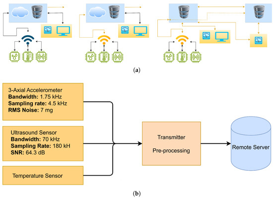
Figure 1.
The cloud-based condition monitoring system. (a) Interconnected devices communicating to a central server. (b) The collection and processing of data from a multi-mode sensor mounted on machinery and transmitting it to a remote server.
The data examined in this paper were collected from an industrial coupled suction (radial) fan that nominally rotates at 3000 rpm at 50 Hz, collecting the dust from the production process to exhaust it to the atmosphere, as can be seen in Figure 2. Since there is a driver–controller (typical PID) that adjusts the rotation speed of the motor according to the amount of dust to be collected (i.e., load), the rotation speed, as will be shown in forthcoming sections, is time-varying. The rotation speed is estimated by detecting the peak with the greatest magnitude around a given rotation speed range, typically [3000, 4200] rpm ([50, 70] Hz) in the velocity spectrum. This method is subject to a certain level of error that can be neglected given the methods employed in this work. The sensor is attached to the drive end (DE) of the motor with a double-sided industrial tape, allowing the capture of information-rich signals related to rotor imbalance, rotor blade faults, bearing (6313 ZZ/C3) defects, and possibly loose or abrasive bearing housing.
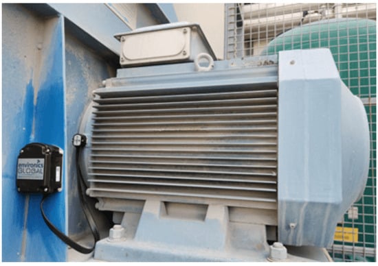
Figure 2.
Industrial coupled suction (radial) fan that nominally rotates at 3000 rpm with the multi-sensor attached on the drive end.
The data consists of the following estimates: rotation speed (rpm), surface temperature (celcius), ultrasound level (dB), 3D kurtosis, 3D peak acceleration, 3D RMS acceleration (g), 3D vibration speed (mm/s), and classification level. The rotation speed indicates the shaft rotation speed of the motor, while the surface temperature reflects the heating status of the motor. The ultrasound level indicates the ultrasonic vibrations in the system, and 3D kurtosis describes the sharpness of the signal’s probability density function. Three-dimensional peak acceleration represents the highest acceleration in the vibration signal amplitude, while 3D RMS acceleration represents the overall acceleration level of the signal. Finally, 3D vibration speed represents the velocity derived from the acceleration signal, and the classification level determines whether the signal is produced by a healthy machine or indicates a mechanical fault. These parameters are used to detect anomalies and performance variations in the monitored machine [70]. To begin with, all the signals mentioned above will be represented with their discrete-time counterparts due to the analog-to-digital conversion inherent in the transmitter. A discrete-time zero-mean vector is represented as x[n], where n denotes the total number of elements in the observed dataset, and the kurtosis of the sampled signal is estimated by employing the expectation operator as in Equation (9).
These features capture fault-prone behaviors and dynamic (and highly non-linear) interactions that are essential parts of the machinery’s operational state. The temporal dynamics of these aspects are highlighted in Figure 3, which shows how variables including vibration acceleration, vibration velocity, kurtosis, rotational speed, and ultrasonic levels change over time. The trends and fluctuations highlight industrial systems’ complex and dynamic behavior and the need for sophisticated pre-processing and analytical techniques to gain valuable insights from such complicated data. As mentioned in previous sections, the motor has been driven above 50 Hz during most of the operation time, rotating over its nominal speed and amplifying the imbalance in the rotor. The extra imbalance created in the coupled fan (even though standing on the vibration dampers it) produces improper clearance and concentrated load distribution in the bearing outer race [2], increasing metal–metal contact by destroying the lubrication film oil, which finally increases the ultrasound level.
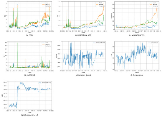
Figure 3.
Temporal trends of key features in the database. (a) Peak values. (b) Vibration acceleration. (c) Vibration velocity. (d) Kurtosis across the axial, vertical, and horizontal axes. (e) Rotation speed. (f) Surface temperature. (g) Ultrasound levels.
The original raw dataset comprised 3413 rows and 24 features. Data pre-preparation was applied to remove redundant readings and outliers, reducing the data sample points. The steps involved in data preparation were as follows: The raw data were pre-processed for missing values, and baseline scaling was applied to numerical features of the import for homogeneity, selecting the information from the features relevant to model training. Noise reduction methods were also implemented to improve signal clarity, given the complex nature of sensor data. Feature engineering has been crucial in extracting any pertinent signal from the raw data; for instance, higher-order statistics—such as but not limited to kurtosis—play an essential role in the fault detection process. Data cleaning ensured that outliers or irrelevant data points were removed, and thus the dataset was prepared for training machine learning models against unnecessary noise and inaccuracies.
As illustrated in Figure 3, the vibration data solely consists of time-domain features without transforming the data into another domain to isolate and focus the study on determining the best-performing classification task on such multi-modal data collected from real working conditions [71]. Improving the data quality through more sophisticated pre-processing steps, denoising approaches, and adding well-known features such as frequency band power estimations are out of the scope of this study and will be subject to examination in future research depending on the availability of data from industry.
Figure 4 provides a comprehensive overview of the distribution of key numerical features through individual box plots, including rotation speed, temperature, kurtosis, peak values, and vibration measurements across axial, vertical, and horizontal directions. Each subplot illustrates the interquartile range (IQR), central tendency (median), spread, whiskers, and outliers. The IQR, representing the middle 50% of the data, provides insight into data variability, while the median indicates the central value. The whiskers extend to cover the majority of data points, and values outside these whiskers are considered outliers, which may indicate anomalies or early-stage faults in the machinery. The spread of the data reveals fluctuations in machine performance; a larger spread indicates higher variability. By comparing different features such as vibration acceleration and ultrasound levels, parameters with higher variability or extreme values can be identified, potentially indicating mechanical issues such as bearing faults or rotor imbalance. This distribution analysis aids in setting thresholds for anomaly detection, enabling predictive maintenance by triggering alerts when machine behavior deviates from normal operating ranges, thus improving fault detection and maintenance planning accuracy.
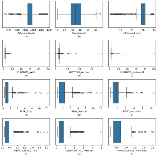
Figure 4.
Distribution of numerical features using box plots: (a) Rotation Speed, (b) Temperature, (c) Ultrasound Level, (d–f) Kurtosis in the axial, vertical, and horizontal axes, (g–i) Peak values in the axial, vertical, and horizontal axes, (j–l) Vibration accelerations in the axial, vertical, and horizontal axes.
The features shown in each subplot of Figure 4 are as follows: (a) rotation speed; (b) temperature, reflecting thermal conditions; (c) ultrasound level, sensitive to minor faults; (d–f) kurtosis values along axial, vertical, and horizontal axes, indicating sharpness in vibration signals and transient faults; (g–i) peak values along the three axes, representing maximum vibration amplitudes, which may signal mechanical stress or faults; and (j–l) vibration acceleration measurements in axial, vertical, and horizontal directions, reflecting dynamic mechanical responses.
3.3. Possible Mechanical Faults to Be Detected in PdM
Mechanical faults that have the potential to cause a breakdown can be listed in two major categories according to their occurrence in the observable frequency range [2,72,73]:
- Low frequency: Considering industrial machinery rotating in a speed range of 10–4000 rpm, mechanical faults that are directly associated with rotation frequency and its harmonics are considered here. These can be given as unbalance in the shaft or fan rotor, turbulence in rotating parts such as fan blades or pump vanes, imbalance of the motor stator/rotor, misalignment in the coupling of bearing races or pulleys, a soft foot, mechanical looseness, a bent shaft, eccentricity, and finally loose belts. Within the collected set of parameters, rotation speed (rpm or Hz) and overall velocity (mm/s) are used to classify these faults [74].
- Rest of the frequency range:
- –
- Mid- and High-Frequency Range: Applying the same considerations on the machinery given at point 1, that is, bearing race defects such as cracks or pits producing periodic impulses exciting the entire frequency range and gear faults, bearing/gear wear and fatigue damage give rise to vibrations in the mid- and high-frequency range. Within the collected set of parameters, peak, peak acceleration, RMS acceleration, as well as Kurtosis are used to classify the faults listed hereby.
- –
- Ultra-High-Frequency Range: Metal–metal contact due to a lack of lubrication, pressurized vapor, or fluid leak, as well as cavitation and subsurface cracks in bearings and gears, produces sound waves above the audible frequency range (>20 kHz). Within the collected set of parameters, the ultrasound RMS level (dB) is used to classify the faults in this category.
The mechanical faults given in Table 2 [3,4,6,10,69] were categorized according to the definitions given above. In any industrial machinery and its common rotating parts—such as bearings and gears—subsurface defects that might start to occur due to the low-frequency failures in point 1 will manifest themselves within the ultrasonic range, as high-frequency shock waves will be generated due to metal–metal contact. Detecting these faults in their early stages would provide a lead time for maintenance personnel. Categorization then proceeds with developed bearing or gear defects and finally ends with low-frequency defects related to shaft rotation.
Table 2.
Fault category with symptoms and possible root causes.
3.4. Model Training and Validation
Data training and validation are conducted with the Python programming language using scikitlearn, XGBoost, LightGBM, matplotlib, seaborn, pandas, and numpy on an Intel Core i7 device with an onboard graphics processor, 512 GB of SSD storage, and 16 GB of RAM.
The MSDCP (Machine learning-based Systematic Dataset Comparison and Prediction) algorithm automates the steps of pre-processing, feature selection, model training, and performance evaluation on a given dataset, aiming to conduct a comparative analysis of different machine learning algorithms. The overall procedure of the MSDCP approach is described in detail in the pseudocode provided in Algorithm 1. The MSDCP function takes four main input parameters: D represents the raw dataset. A denotes the list of algorithms to be evaluated. F refers to the selected features or feature selection criteria, and P indicates the pre-processing settings. During the pre-processing phase, the dataset is prepared based on the specified configurations; subsequently, selected features are used to optimize the dataset. The processed data is then split into the training and testing sets, with 80% allocated for training and 20% for testing. The training data is used to build models, while the test data is reserved for evaluating model performance. In this stage, various machine learning algorithms (e.g., the SVM, the RF, etc.) are trained and tested. To enhance model accuracy, hyperparameter optimization is performed, allowing fine-tuning of the model parameters. The results are ranked based on performance and visualized. The performance outcomes for each algorithm are presented in Table 3, and the overall workflow is depicted in Figure 5.
| Algorithm 1 Pseudocode of MSDCP. |
|
Table 3.
Performance of classification algorithms.
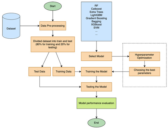
Figure 5.
Flow diagram of the proposed system.
The heatmap visualization in Figure 6 illustrates the interconnections among numerical variables through correlation analysis. The presence of high correlation points to possible redundant features, whereas lower correlation coefficients suggest that certain variables may offer distinct information for fault classification purposes. It would be beneficial to elaborate on how these correlation patterns guide research decisions in feature selection and their subsequent effects on the model’s effectiveness. The following section builds on these findings by examining the resulting classification performance across different algorithms.
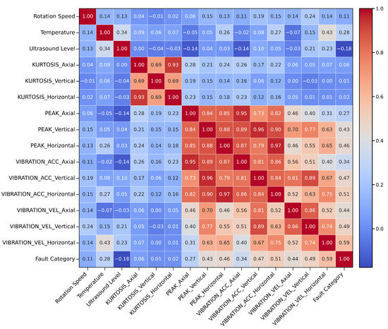
Figure 6.
Correlation heatmap.
4. Results
Table 3 presents a comparative analysis of various classification algorithms for fault detection in rotating machinery, evaluated based on accuracy, precision, recall, F1 scores, and execution times. Among the tested models, the Random Forest stood out not only in classification accuracy (0.768) but also in efficiency, with a notably fast execution time of 0.953 s, followed closely by CatBoost (0.765) and extra trees (0.755). However, the CatBoost model showed a disadvantage in terms of execution time. These ensemble techniques seem to be more effective than the remaining models, which show comparably better performance in fault classification tasks. In contrast, simpler models, such as the ridge classifier (0.624), K-Nearest Neighbors (0.676), and Linear SVC (0.670), reported average accuracy, which suggests that these algorithms could not handle the complexity or non-linearity of the given dataset.
The boosting algorithms LightGBM (0.752), bagging (0.743), and Gradient Boosting (0.731) demonstrated varied levels of performance. Their performances were slightly lower than any of the aforementioned ensemble methods, likely due to greater sensitivity to noise in the dataset. In contrast, Gradient Boosting (0.731), XGBoost (0.715), and the SVM (0.713) achieved moderate performance, indicating their effectiveness but slightly lower generalization capabilities. On the lower end, the decision tree (0.682), K-Nearest Neighbors (0.676), Linear SVC (0.670), and SGD (0.627) displayed average classification abilities, while AdaBoost (0.532) performed the worst, likely due to its sensitivity to noisy data. Overall, the results highlight that ensemble-based models, particularly the Random Forest, are the most effective for fault detection in the given rotating machinery, offering relatively higher accuracy and reliability.
After performance measurement with default values, hyperparameter optimization was conducted for all classifiers using grid search with 5-fold cross-validation. The tuned results are summarized in Table 4. Among the models, the Random Forest achieved the highest classification accuracy (0.771). The Random Forest classifier performs considerably better because it is an ensemble learning method composed of many decision trees. This structure reduces the probability of overfitting compared to individual trees and enhances robustness and stability when handling complex datasets. It brings in randomness at two levels, namely at the level of training data and at the level of features used to build each tree, which ensures diversity in trees and hence better generalization. Besides that, the Random Forest has the capability of evaluating the importance of individual features, which can guide feature selection and improve efficiency. It can cope with large datasets featuring many attributes and avoids overfitting by averaging predictions across multiple trees, making it extremely valuable for handling noisy or high-dimensional data.
Table 4.
Performance comparison of classification models after hyperparameter optimization.
Right after the Random Forest, CatBoost (0.769) and Gradient Boosting (0.763) followed closely. Notably, Gradient Boosting and the bagging classifier, after tuning, showed a marked improvement to an accuracy of 0.763 and 0.761, indicating that they may compete closely with the Random Forest. While CatBoost and XGBoost performed well in terms of accuracy, their significantly higher execution times (870.3 s and 306.5 s, respectively) may limit their suitability for time-sensitive applications. Simpler models such as the decision tree, K-Nearest Neighbors, and the SVM benefited modestly from optimization, yet they were still outperformed by ensemble and boosting techniques. AdaBoost, despite tuning, remained the least effective model, likely due to its sensitivity to noise. These results confirm the importance of hyperparameter tuning and demonstrate that ensemble-based methods, particularly the Random Forest and the bagging classifier, provide robust performance for multi-sensor fault classification tasks under real-world industrial conditions.
A comprehensive range of values was evaluated for each parameter, as presented in Table 5, which also summarizes optimal hyperparameter settings for the Random Forest classifier. These values were selected based on their average validation accuracy scores across the five cross-validation folds. The model performed best with 1000 estimators, indicating that increasing the number of decision trees improves model stability and accuracy by significantly reducing variance. In the Random Forest algorithm, the parameter defines the maximum depth each individual decision tree can grow. Setting it to 10 strikes a reasonable balance between model complexity and the risk of overfitting: deeper trees may overfit the training data, while shallower trees may underfit and fail to capture relevant patterns.
Table 5.
Parameters and best values of RF classifier algorithms with hyperparameter optimization.
The selected values for and indicate that the model is capable of splitting nodes as long as there are at least two samples available, with leaf nodes containing at least one sample. This configuration allows for more detailed splits, thereby enhancing the model’s ability to capture complex patterns without sacrificing accuracy. Additionally, setting ensures that feature selection is performed randomly, which introduces diversity and mitigates the risk of overfitting.
By setting the bootstrap parameter to True, the model can utilize bootstrapped sampling, a core feature of the Random Forest in variance reduction. The Gini criterion was chosen as a measure of the impurity of the nodes, which reflects class homogeneity in the splitting. There were no inputs such as class_weight and max_samples that might signify a balanced dataset that would not require weighting.
To summarize, these hyperparameter values exemplify a well-tuned Random Forest model optimally aligned for stability and generalization. The trees are relatively deep. The number of estimators is high, and the feature selection is random. Together, they contribute to the robustness of the model in classifying faults. To further validate the impact of hyperparameter optimization, we conducted a paired t-test comparing the 5-fold cross-validation accuracy scores of the default and optimized Random Forest models. Prior to the test, the normality of the differences was assessed using the Shapiro–Wilk test (), confirming that the distribution of differences satisfies the normality assumption. The paired t-test revealed a statistically significant improvement in accuracy (, ), based on a significance level of 0.05, supporting the effectiveness of the optimization strategy.
The SHAP-based feature importance analysis (Figure 7) provides a detailed understanding of how individual variables contribute to the classification performance across different fault categories. In particular, features such as VIBRATION_VEL_Vertical (mm/s), VIBRATION_VEL_Horizontal (mm/s), and ultrasound Level (dB) exhibited the highest mean absolute SHAP values, indicating their consistent and dominant influence on the model’s decision-making process. Furthermore, the distribution of SHAP values across multiple classes suggests that certain features play more prominent roles in specific fault types, highlighting the class-dependent relevance of input variables. For example, VIBRATION_VEL_Vertical (mm/s) and VIBRATION_VEL_Horizontal (mm/s) were especially influential in the prediction of Class 0, Class 2, and Class 5, whereas their contribution was relatively lower for Class 6 and Class 7. In contrast, features such as KURTOSIS_Horizontal, KURTOSIS_Vertical, and rotation speed had minimal influence, suggesting that they play a lesser role in the classification decisions.
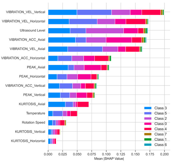
Figure 7.
Mean absolute SHAP values for the optimized RF model.
These findings highlight the importance of domain-specific features such as deflection speed and the effective capture of fault patterns. The SHAP analysis also reveals that some features are consistently informative across fault types, while others contribute minimally and can often be excluded. This supports the potential for dimensionality reduction and simplified models that are efficient enough for real-time applications without sacrificing accuracy.
Moreover, the dominance of vibration velocity and ultrasound levels in feature importance as depicted in Figure 7 aligns with mechanical fault mechanisms: velocity signals reflect rotor imbalance (low-frequency faults), while ultrasound spikes indicate early bearing wear [2,35]. The superiority of the Random Forest stems from its inherent noise tolerance, whereas AdaBoost’s sensitivity to label noise explains its lower accuracy. Notably, the real-world accuracy (76.8%) obtained in this study is lower than lab-based studies [9], underscoring the challenges of industrial data variability.
Figure 8 shows both training and validation accuracy scores of the Random Forest classifier that can generalize relatively better against unseen data. The validation set is a subset of the data that is separate from the training and test sets, used during the training process to tune hyperparameters and assess the model’s ability to generalize to unseen data. Validation accuracy is used to monitor the model’s performance during training and help prevent overfitting, ensuring that the model does not memorize the training data but instead learns to generalize well to new, unseen data. The training and validation scores were approximately similar, with no overfitting or underfitting. This indicates a well-tuned hyperparameter setting. The accuracy has leveled off to a relatively higher score, which means that the model has learned considerably well from the dataset, and also the data has been enough for the classification problem. It also certifies that the Random Forest can be considered a good candidate for fault detection and prediction on multi-sensor data, while the minor difference between the scores further strengthens the robustness of the model. Future work could focus on upscaling certain metrics through cross-validation or other ensemble techniques to improve performance.
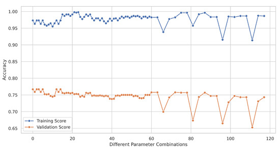
Figure 8.
Training and validation accuracy scores.
The final dataset used in this study consists of 1631 labeled samples, obtained after thorough data cleaning and pre-processing, including removing missing entries. The confusion matrix shown in Figure 9 was generated using the optimized Random Forest model, which was trained using 5-fold cross-validation during hyperparameter tuning. However, these results specifically reflect the performance on the held-out test set, derived from an 80/20 split after shuffling the dataset. This test set was not used during model training or validation, ensuring that the confusion matrix truly represents the model’s generalization performance. Each row represents the true class, and each column represents the predicted class, with the values in the matrix indicating the number of occurrences. The diagonal elements (e.g., 29 for Class 0, 69 for Class 3, and 73 for Class 5) represent the correctly classified instances, indicating good model performance on these classes. However, several misclassifications are evident, especially for certain classes like Class 4 (15 correctly classified and 29 misclassified), Class 2 (46 correctly classified and 5 misclassified), and Class 7 (only 1 predicted correctly). These misclassifications suggest that the model struggles more with certain fault categories, possibly due to class imbalance or the subtle differences between classes. Additionally, the model performs better with larger classes, such as Class 5, which has a large number of samples, compared to smaller classes with fewer samples, leading to potential bias toward the majority class.
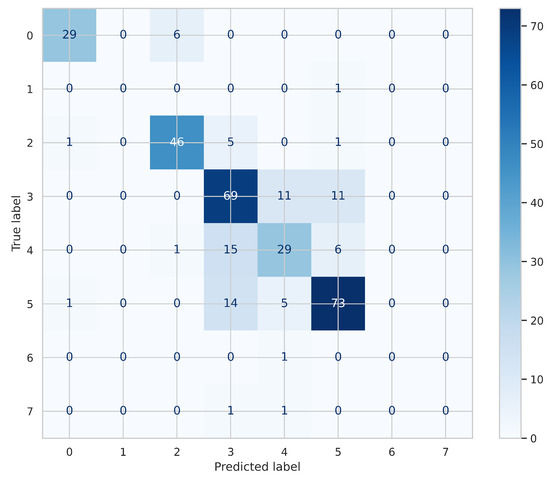
Figure 9.
Confusion matrix showing the optimized Random Forest model performance across fault categories.
The distribution of the labeled data across the eight fault categories is as follows: Class 3 (vibration impulses) contains 474 samples. Class 5 (rotation frequency and harmonics) has 452 samples. Class 2 (wideband vibration impulses) has 263 samples, and Class 4 (high-frequency vibrations) includes 231 samples. In comparison, Class 0 (ultrasonic level) consists of 180 samples, while Class 1, Class 7, and Class 6 are severely underrepresented with only 12, 14, and 5 samples, respectively. This class imbalance is an important factor that affects model performance, particularly for minority classes, and explains the misclassifications observed in the confusion matrix.
5. Conclusions
This paper presents a comparative study on the performance of various machine learning algorithms for fault detection in rotating machines, using multi-modal data collected from real-world conditions in a typical manufacturing industry. The dataset comprises approximately one-year-long organic data, acquired from a coupled suction fan. Our results have shown that the Random Forest classifier achieved the highest accuracy of 77.1%, followed by the CatBoost and Gradient Boosting with 76.9% and 76.3% respectively.
Hyperparameter optimization has resulted in a slight improvement, as the labels used in this study require derived features from the frequency-domain transformation of the raw vibration and ultrasound signals. The original feature space, consisting mostly of time-domain features, is not powerful enough to discriminate the cases, and even the optimized models may perform poorly. Additionally, correlated features may introduce noise rather than contribute representative information. To account for this, alternatives such as iterative feature elimination, mutual information-based selection, or dimensionality reduction (e.g., PCA) can be used to retain only informative features. A possible future study will focus on estimating the Fourier representation of the collected observations with different approaches and inferring the data to re-evaluate the optimization schemes, which are expected to yield better performance. For the sake of clarity and simplicity of the presentation on the available data, only time-domain features in vibration analysis, the highest frequency range of the ultrasound RMS level, revolution speed, and temperature were used in this study. Nevertheless, it has been shown that even without time-dependent and band-selective frequency power (simply short-time Fourier transform) information, the classification algorithms proved a relatively satisfactory performance given the simple raw data indexes from acceleration and ultrasound signals.
Notably, although the observed improvement in classification accuracy through hyperparameter tuning was statistically significant (paired t-test, ), the magnitude of this improvement remains limited. This outcome highlights the importance of more informative and discriminative feature sets to fully leverage the benefits of model optimization. Despite this limitation, the classification system was still able to detect underlying patterns associated with mechanical faults.
In particular, the aforementioned imbalance and its indirect effect of bearing wear were successfully identified, yielding a system that could automatically detect mechanical failures. The importance list of features in Figure 7 proves the fact that the fault-related parameters, velocity, and ultrasound contribute to the classification at a considerably higher level, in line with the observations and expectations.
Limitations
As it is briefly discussed in previous sections, even though the presented framework demonstrates promise on industrial rotating machinery condition monitoring, several limitations can be mentioned. First, the reliance on time-domain features especially on mid- and high-frequency ranges of vibration signals may restrict fault discrimination for high-frequency failures (e.g., bearing spalls and gear cracks), which are better captured by frequency-domain analyses. Second, the model’s validation on a single machine type (coupled radial suction fan) necessitates caution in generalizing to other rotating equipment. In addition to that, the machinery subjected to analysis here rotates above 3000 rpm, excluding relatively harder cases on slowly rotating machinery, that is, below 60 rpm. Future work will integrate multi-domain features and expand datasets to address these gaps.
6. Open Issues & Future Works
The dataset examined in this work demonstrates the complicated relation between observed parameters in industrial rotating machinery, which possesses considerable difficulties due to its non-linear structure and strong feature correlations. Reducing unexpected downtime and unscheduled repairs, optimizing maintenance, and preserving operational safety depend on efficient and accurate defect detection. Although it is relatively easy to collect and process data using modern sensors and communication technologies, it can be challenging to retrieve useful information from this multi-modal, inherently noisy data. In a possible pre-processing step, unsupervised learning approaches are crucial because they can increase the SNR, which can improve future analysis and signal clarity [46,47]. By leveraging labeled data, supervised methods aim to deliver actionable insights that directly support predictive maintenance strategies. These techniques help prepare the data for downstream applications, bridging the gap between analyzing raw sensor data and advanced analytical models. To provide useful insights for predictive maintenance, this paper offers an empirical examination of various supervised learning techniques using real-world industrial data obtained via low-cost, low-power LoRa-WAN devices.
To improve the accuracy and robustness of the model, future studies could investigate combining data from several frequency bands within the acceleration and ultrasound range. LSTMs and CNNs offer promising approaches for identifying temporal and spatial patterns in the data. LSTMs are well-suited to capture sequential dependencies that show the progression of faults, but CNNs are capable of identifying crucial spatial features. Simplifying sensor positioning and data collection techniques may help to further enhance input data quality and boost model performance as a whole. Combining these methods with localized devices in real-time monitoring systems may result in faster reactions and more immediate on-site insights.
Furthermore, by using transfer learning, models may be able to generalize across various datasets or types of machinery, decreasing the requirement for large amounts of labeled data while increasing applicability. These developments are anticipated to make a substantial contribution to the field of intelligent detection as well as to the wider industrial use of predictive maintenance solutions.
Author Contributions
Conceptualization, T.K. and S.B.; methodology, S.D.; software, M.Y.; validation, M.Y. and A.K.O.; formal analysis, S.B.; investigation, T.K. and S.B.; resources, T.K. and S.B.; data curation, M.Y.; writing—original draft preparation, T.K., S.B., A.K.O., M.Y., and S.D.; writing—review and editing, T.K., S.B., A.K.O., M.Y., and S.D.; visualization, S.D. and M.Y.; supervision, A.K.O.; project administration, A.K.O. All authors have read and agreed to the published version of the manuscript.
Funding
The APC (Article Processing Charge) for this manuscript is funded by the authors.
Institutional Review Board Statement
Not applicable.
Informed Consent Statement
Not applicable.
Data Availability Statement
The data used in this study are not publicly available due to restrictions imposed by non-disclosure agreements (NDAs).
Conflicts of Interest
The authors declare no conflicts of interest.
References
- Sunetcioglu, S.; Arsan, T. Predictive Maintenance Analysis for Industries. In Proceedings of the 2024 IEEE International Black Sea Conference on Communications and Networking (BlackSeaCom), Tbilisi, Georgia, 24–27 June 2024; pp. 344–347. [Google Scholar] [CrossRef]
- Yang, Y.; Hu, P.; Luo, J.; An, Z.; Cao, J.; Yu, D.; Cheng, X. Romeo: Fault Detection of Rotating Machinery via Fine-Grained mmWave Velocity Signature. IEEE Trans. Mob. Comput. 2025, 24, 227–242. [Google Scholar] [CrossRef]
- Romanssini, M.; de Aguirre, P.C.C.; Compassi-Severo, L.; Girardi, A.G. A review on vibration monitoring techniques for predictive maintenance of rotating machinery. Eng 2023, 4, 1797–1817. [Google Scholar] [CrossRef]
- Sicard, B.; Alsadi, N.; Spachos, P.; Ziada, Y.; Gadsden, S.A. Predictive Maintenance and Condition Monitoring in Machine Tools: An IoT Approach. In Proceedings of the 2022 IEEE International IOT, Electronics and Mechatronics Conference (IEMTRONICS), Toronto, ON, Canada, 1–4 June 2022; pp. 1–9. [Google Scholar] [CrossRef]
- Pinheiro, A.A.; Brandao, I.M.; Da Costa, C. Vibration analysis in turbomachines using machine learning techniques. Eur. J. Eng. Technol. Res. 2019, 4, 12–16. [Google Scholar]
- Anwarsha, A.; Narendiranath Babu, T. Recent advancements of signal processing and artificial intelligence in the fault detection of rolling element bearings: A review. J. Vibroeng. 2022, 24, 1027–1055. [Google Scholar] [CrossRef]
- Huynh, H.H.; Min, C.H. Rotating Machinery Fault Detection Using Support Vector Machine via Feature Ranking. Algorithms 2024, 17, 441. [Google Scholar] [CrossRef]
- Singh, G.; Sundaram, K. Methods to improve wind turbine generator bearing temperature imbalance for onshore wind turbines. Wind Eng. 2022, 46, 150–159. [Google Scholar] [CrossRef]
- Pan, H.; He, X.; Tang, S.; Meng, F. An improved bearing fault diagnosis method using one-dimensional CNN and LSTM. J. Mech. Eng./Stroj. Vestn. 2018, 64, 443–453. [Google Scholar]
- Chu, T.; Nguyen, T.; Yoo, H.; Wang, J. A review of vibration analysis and its applications. Heliyon 2024, 10, e26282. [Google Scholar] [CrossRef]
- Tahmasbi, D.; Shirali, H.; Souq, S.S.M.N.; Eslampanah, M. Diagnosis and root cause analysis of bearing failure using vibration analysis techniques. Eng. Fail. Anal. 2024, 158, 107954. [Google Scholar] [CrossRef]
- Lv, Y.; Liu, H.; Chen, Z.; Chang, W.; Zhang, H.; Li, H. Lubrication condition monitoring of journal bearings in diesel engine based on thermoelectricity. Friction 2024, 12, 2532–2547. [Google Scholar] [CrossRef]
- Zhu, J.; Gao, H.-L.; Liu, C.; Wang, L.; Yu, J. Experimental study on monitoring the wear of journal bearings of diesel engine by thermoelectric method. DEStech Trans. Environ. Energy Earth Sci. 2018, 166–171. [Google Scholar] [CrossRef] [PubMed]
- Zhu, J.; Gao, H.l.; Pi, D.n.; Xie, Z.q.; Mei, L. Thermoelectric effect of wear of alloy bearing. Eng. Fail. Anal. 2019, 103, 376–383. [Google Scholar] [CrossRef]
- Zhou, P.; Chen, S.; He, Q.; Wang, D.; Peng, Z. Rotating machinery fault-induced vibration signal modulation effects: A review with mechanisms, extraction methods and applications for diagnosis. Mech. Syst. Signal Process. 2023, 200, 110489. [Google Scholar] [CrossRef]
- Zhang, Z.; Huang, W.; Liao, Y.; Song, Z.; Shi, J.; Jiang, X.; Shen, C.; Zhu, Z. Bearing fault diagnosis via generalized logarithm sparse regularization. Mech. Syst. Signal Process. 2022, 167, 108576. [Google Scholar] [CrossRef]
- Lei, Y.; Yang, B.; Jiang, X.; Jia, F.; Li, N.; Nandi, A.K. Applications of machine learning to machine fault diagnosis: A review and roadmap. Mech. Syst. Signal Process. 2020, 138, 106587. [Google Scholar] [CrossRef]
- Duan, L.; Xie, M.; Wang, J.; Bai, T. Deep learning enabled intelligent fault diagnosis: Overview and applications. J. Intell. Fuzzy Syst. 2018, 35, 5771–5784. [Google Scholar] [CrossRef]
- Liu, R.; Yang, B.; Zio, E.; Chen, X. Artificial intelligence for fault diagnosis of rotating machinery: A review. Mech. Syst. Signal Process. 2018, 108, 33–47. [Google Scholar] [CrossRef]
- Jiang, L.l.; Yin, H.k.; Li, X.j.; Tang, S.w. Fault Diagnosis of Rotating Machinery Based on Multisensor Information Fusion Using SVM and Time-Domain Features. Shock Vib. 2014, 2014, 418178. [Google Scholar] [CrossRef]
- Xia, M.; Li, T.; Xu, L.; Liu, L.; De Silva, C.W. Fault diagnosis for rotating machinery using multiple sensors and convolutional neural networks. IEEE/ASME Trans. Mechatron. 2017, 23, 101–110. [Google Scholar] [CrossRef]
- Cao, H.; Shao, H.; Liu, B.; Cai, B.; Cheng, J. Clustering-guided novel unsupervised domain adversarial network for partial transfer fault diagnosis of rotating machinery. IEEE Sens. J. 2022, 22, 14387–14396. [Google Scholar] [CrossRef]
- Sun, W.; Shao, S.; Zhao, R.; Yan, R.; Zhang, X.; Chen, X. A sparse auto-encoder-based deep neural network approach for induction motor faults classification. Measurement 2016, 89, 171–178. [Google Scholar] [CrossRef]
- Yin, A.; Yan, Y.; Zhang, Z.; Li, C.; Sánchez, R.V. Fault diagnosis of wind turbine gearbox based on the optimized LSTM neural network with cosine loss. Sensors 2020, 20, 2339. [Google Scholar] [CrossRef]
- Lee, X.Y.; Kumar, A.; Vidyaratne, L.; Rao, A.R.; Farahat, A.; Gupta, C. An ensemble of convolution-based methods for fault detection using vibration signals. In Proceedings of the 2023 IEEE International Conference on Prognostics and Health Management (ICPHM), Montreal, QC, Canada, 5–7 June 2023; pp. 172–179. [Google Scholar]
- Biot-Monterde, V.; Navarro-Navarro, A.; Zamudio-Ramirez, I.; Antonino-Daviu, J.A.; Osornio-Rios, R.A. Automatic classification of rotor faults in soft-started induction motors, based on persistence spectrum and convolutional neural network applied to stray-flux signals. Sensors 2022, 23, 316. [Google Scholar] [CrossRef] [PubMed]
- Xiong, J.; Zhang, Q.; Peng, Z.; Sun, G.; Xu, W.; Wang, Q. A Diagnosis Method for Rotation Machinery Faults Based on Dimensionless Indexes Combined with K-Nearest Neighbor Algorithm. Math. Probl. Eng. 2015, 2015, 563954. [Google Scholar] [CrossRef]
- Hassan, M.A.; Habib, M.R.; Abul Seoud, R.A.; Bayoumi, A.M. Wavelet-based multiresolution bispectral analysis for detection and classification of helicopter drive-shaft problems. J. Dyn. Syst. Meas. Control 2018, 140, 061009. [Google Scholar] [CrossRef]
- Das, O.; Das, D.B.; Birant, D. Machine learning for fault analysis in rotating machinery: A comprehensive review. Heliyon 2023, 9, e17584. [Google Scholar] [CrossRef]
- Gawde, S.; Patil, S.; Kumar, S.; Kotecha, K. A scoping review on multi-fault diagnosis of industrial rotating machines using multi-sensor data fusion. Artif. Intell. Rev. 2023, 56, 4711–4764. [Google Scholar] [CrossRef]
- Ho, D.; Randall, R.B. Optimization of bearing diagnostic techniques using simulated and actual bearing fault signals. Mech. Syst. Signal Process. 2000, 14, 763–788. [Google Scholar] [CrossRef]
- Mallikarjuna, P.; Sreenatha, M.; Manjunath, S.; Kundur, N.C. Aircraft gearbox fault diagnosis system: An approach based on deep learning techniques. J. Intell. Syst. 2020, 30, 258–272. [Google Scholar] [CrossRef]
- Cao, L.; Qian, Z.; Zareipour, H.; Huang, Z.; Zhang, F. Fault diagnosis of wind turbine gearbox based on deep bi-directional long short-term memory under time-varying non-stationary operating conditions. IEEE Access 2019, 7, 155219–155228. [Google Scholar] [CrossRef]
- Hasan, M.J.; Rai, A.; Ahmad, Z.; Kim, J.M. A fault diagnosis framework for centrifugal pumps by scalogram-based imaging and deep learning. IEEE Access 2021, 9, 58052–58066. [Google Scholar] [CrossRef]
- Tiwari, R.; Bordoloi, D.; Dewangan, A. Blockage and cavitation detection in centrifugal pumps from dynamic pressure signal using deep learning algorithm. Measurement 2021, 173, 108676. [Google Scholar] [CrossRef]
- Hu, D.; Zhang, C.; Yang, T.; Chen, G. An Intelligent Anomaly Detection Method for Rotating Machinery Based on Vibration Vectors. IEEE Sens. J. 2022, 22, 14294–14305. [Google Scholar] [CrossRef]
- Randall, R.B.; Antoni, J. Rolling element bearing diagnostics—A tutorial. Mech. Syst. Signal Process. 2011, 25, 485–520. [Google Scholar] [CrossRef]
- Rai, A.; Upadhyay, S.H. A review on signal processing techniques utilized in the fault diagnosis of rolling element bearings. Tribol. Int. 2016, 96, 289–306. [Google Scholar] [CrossRef]
- Ozkat, E.C. A Degradation Model to Predict the Remaining Useful Life of Bearings. In Proceedings of the International Conference on AI and Big Data in Engineering Applications, Istanbul, Turkey, 14–15 June 2021; p. 227. [Google Scholar]
- Shandhoosh, V.; Chakrapani, G.; Sugumaran, V.; Ramteke, S.M.; Marian, M. Intelligent fault diagnosis for tribo-mechanical systems by machine learning: Multi-feature extraction and ensemble voting methods. Knowl.-Based Syst. 2024, 305, 112694. [Google Scholar] [CrossRef]
- Neupane, D.; Bouadjenek, M.R.; Dazeley, R.; Aryal, S. A Comparative Study of Semi-Supervised Anomaly Detection Methods for Machine Fault Detection. PHM Soc. Eur. Conf. 2024, 8, 10. [Google Scholar] [CrossRef]
- Kim, M.; Jung, J.H.; Ko, J.U.; Kong, H.B.; Lee, J.; Youn, B.D. Direct connection-based convolutional neural network (DC-CNN) for fault diagnosis of rotor systems. IEEE Access 2020, 8, 172043–172056. [Google Scholar] [CrossRef]
- Yuan, X.; He, Y.; Wan, S.; Qiu, M.; Jiang, H. Remote vibration monitoring and fault diagnosis system of synchronous motor based on internet of things technology. Mob. Inf. Syst. 2021, 2021, 3456624. [Google Scholar] [CrossRef]
- Chang, H.C.; Wang, Y.C.; Shih, Y.Y.; Kuo, C.C. Fault Diagnosis of Induction Motors with Imbalanced Data Using Deep Convolutional Generative Adversarial Network. Appl. Sci. 2022, 12, 4080. [Google Scholar] [CrossRef]
- Morales, E.F.; Escalante, H.J. A brief introduction to supervised, unsupervised, and reinforcement learning. In Biosignal Processing and Classification Using Computational Learning and Intelligence; Elsevier: Amsterdam, The Netherlands, 2022; pp. 111–129. [Google Scholar]
- Ovacıklı, A.K.; Pääjärvi, P.; LeBlanc, J.P.; Carlson, J.E. Recovering periodic impulsive signals through skewness maximization. IEEE Trans. Signal Process. 2015, 64, 1586–1596. [Google Scholar] [CrossRef]
- Sawalhi, N.; Randall, R.; Endo, H. The enhancement of fault detection and diagnosis in rolling element bearings using minimum entropy deconvolution combined with spectral kurtosis. Mech. Syst. Signal Process. 2007, 21, 2616–2633. [Google Scholar] [CrossRef]
- Roy, S.; Meena, T.; Lim, S.J. Demystifying supervised learning in healthcare 4.0: A new reality of transforming diagnostic medicine. Diagnostics 2022, 12, 2549. [Google Scholar] [CrossRef]
- Boateng, E.Y.; Otoo, J.; Abaye, D.A. Basic tenets of classification algorithms K-nearest-neighbor, support vector machine, random forest and neural network: A review. J. Data Anal. Inf. Process. 2020, 8, 341–357. [Google Scholar] [CrossRef]
- Maxwell, A.E.; Warner, T.A.; Fang, F. Implementation of machine-learning classification in remote sensing: An applied review. Int. J. Remote Sens. 2018, 39, 2784–2817. [Google Scholar] [CrossRef]
- Shrestha, A.; Mahmood, A. Review of deep learning algorithms and architectures. IEEE Access 2019, 7, 53040–53065. [Google Scholar] [CrossRef]
- Zhang, S. Challenges in KNN classification. IEEE Trans. Knowl. Data Eng. 2021, 34, 4663–4675. [Google Scholar] [CrossRef]
- Bithas, P.S.; Michailidis, E.T.; Nomikos, N.; Vouyioukas, D.; Kanatas, A.G. A survey on machine-learning techniques for UAV-based communications. Sensors 2019, 19, 5170. [Google Scholar] [CrossRef]
- Chelgani, S.C.; Homafar, A.; Nasiri, H. CatBoost-SHAP for modeling industrial operational flotation variables–A “conscious lab” approach. Miner. Eng. 2024, 213, 108754. [Google Scholar] [CrossRef]
- Mohammed, A.; Kora, R. A comprehensive review on ensemble deep learning: Opportunities and challenges. J. King Saud Univ.-Comput. Inf. Sci. 2023, 35, 757–774. [Google Scholar] [CrossRef]
- Zhang, Y.; Liu, J.; Shen, W. A review of ensemble learning algorithms used in remote sensing applications. Appl. Sci. 2022, 12, 8654. [Google Scholar] [CrossRef]
- John, V.; Liu, Z.; Guo, C.; Mita, S.; Kidono, K. Real-time lane estimation using deep features and extra trees regression. In Proceedings of the Image and Video Technology: 7th Pacific-Rim Symposium, PSIVT 2015, Auckland, New Zealand, 25–27 November 2015; pp. 721–733. [Google Scholar]
- Ahmad, M.W.; Reynolds, J.; Rezgui, Y. Predictive modelling for solar thermal energy systems: A comparison of support vector regression, random forest, extra trees and regression trees. J. Clean. Prod. 2018, 203, 810–821. [Google Scholar] [CrossRef]
- Nasiri, H.; Dadashi, A.; Azadi, M. Machine learning for fatigue lifetime predictions in 3D-printed polylactic acid biomaterials based on interpretable extreme gradient boosting model. Mater. Today Commun. 2024, 39, 109054. [Google Scholar] [CrossRef]
- Mienye, I.D.; Sun, Y. A survey of ensemble learning: Concepts, algorithms, applications, and prospects. IEEE Access 2022, 10, 99129–99149. [Google Scholar] [CrossRef]
- Chen, T.; Guestrin, C. Xgboost: A scalable tree boosting system. In Proceedings of the 22nd ACM SIGKDD International Conference on Knowledge Discovery and Data Mining, San Francisco, CA, USA, 13–17 August 2016; pp. 785–794. [Google Scholar]
- Ke, G.; Meng, Q.; Finley, T.; Wang, T.; Chen, W.; Ma, W.; Ye, Q.; Liu, T.Y. Lightgbm: A highly efficient gradient boosting decision tree. Adv. Neural Inf. Process. Syst. 2017, 30. [Google Scholar]
- Rozikin, C.; Buono, A.; Arif, C.; Wahjuni, S. Classification of the Severity of Downy Mildew Disease Using LGBM. In Proceedings of the 2023 International Conference on Informatics, Multimedia, Cyber and Informations System (ICIMCIS), Jakarta Selatan, Indonesia, 7–8 November 2023; pp. 364–368. [Google Scholar]
- Prokhorenkova, L.; Gusev, G.; Vorobev, A.; Dorogush, A.V.; Gulin, A. CatBoost: Unbiased boosting with categorical features. Adv. Neural Inf. Process. Syst. 2018, 31. [Google Scholar]
- Liu, H.; Guo, L.; Li, H.; Zhang, W.; Bai, X. Matching areal entities with CatBoost ensemble method. Geogr. Inf. Sci 2022, 24, 2198–2211. [Google Scholar]
- Bischl, B.; Binder, M.; Lang, M.; Pielok, T.; Richter, J.; Coors, S.; Thomas, J.; Ullmann, T.; Becker, M.; Boulesteix, A.L.; et al. Hyperparameter optimization: Foundations, algorithms, best practices, and open challenges. Wiley Interdiscip. Rev. Data Min. Knowl. Discov. 2023, 13, e1484. [Google Scholar] [CrossRef]
- Fristiana, A.H.; Alfarozi, S.A.I.; Permanasari, A.E.; Pratama, M.; Wibirama, S. A Survey on Hyperparameters Optimization of Deep Learning for Time Series Classification. IEEE Access 2024, 12, 191162–191198. [Google Scholar] [CrossRef]
- Ovacıklı, A.K.; Carlson, J.E.; Pääjärvi, P. Blind pulse compression through skewness maximization on overlapping echoes from thin layers. In Proceedings of the 2016 IEEE International Ultrasonics Symposium (IUS), Tours, France, 18–21 September 2016; pp. 1–4. [Google Scholar]
- Asystom Predictive Maintenance Systems. Available online: https://www.asystom.com/ (accessed on 11 May 2025).
- Mohd Ghazali, M.H.; Rahiman, W. Vibration analysis for machine monitoring and diagnosis: A systematic review. Shock Vib. 2021, 2021, 9469318. [Google Scholar] [CrossRef]
- Kullu, O.; Cinar, E. A deep-learning-based multi-modal sensor fusion approach for detection of equipment faults. Machines 2022, 10, 1105. [Google Scholar] [CrossRef]
- Chen, Y.; Chen, Q.; Wang, R. Bearing Fault Diagnosis Based on Vibration Envelope Spectral Characteristics. Appl. Sci. 2025, 15, 2240. [Google Scholar] [CrossRef]
- Ju, T.; Findikoglu, A.T. Large Area Detection of Microstructural Defects with Multi-Mode Ultrasonic Signals. Appl. Sci. 2022, 12, 2082. [Google Scholar] [CrossRef]
- Arora, J.K.; Rajagopalan, S.; Singh, J.; Purohit, A. Low-frequency adaptation-deep neural network-based domain adaptation approach for shaft imbalance fault diagnosis. J. Vib. Eng. Technol. 2024, 12, 375–394. [Google Scholar] [CrossRef]
Disclaimer/Publisher’s Note: The statements, opinions and data contained in all publications are solely those of the individual author(s) and contributor(s) and not of MDPI and/or the editor(s). MDPI and/or the editor(s) disclaim responsibility for any injury to people or property resulting from any ideas, methods, instructions or products referred to in the content. |
© 2025 by the authors. Licensee MDPI, Basel, Switzerland. This article is an open access article distributed under the terms and conditions of the Creative Commons Attribution (CC BY) license (https://creativecommons.org/licenses/by/4.0/).