Multi-Region OpenFOAM Solver Development for Compact Toroid Transport in Drift Tube

Abstract

Compact toroid (CT) injection, with its characteristics of high plasma density and extremely high injection velocity, is considered a highly promising method for core fueling in fusion reactors. Previous studies have lacked investigation into the transport process of CT within drift tubes. To investigate the dynamic processes of CT in drift tubes, this study developed a compressible magnetohydrodynamics (MHD) solver and a magnetic diffusion solver based on the OpenFOAM platform. They were integrated into a multi-region coupling framework to create a multi-region coupled MHD solver, mhdMRF, for simulating the dynamic behavior of CT in drift tubes and its interaction with finite-resistivity walls. The solver demonstrated excellent performance in simulations of the Orszag–Tang MHD vortex problem, the Brio–Wu shock tube problem, analytical verification of magnetic diffusion, and validation of internal coupling boundary conditions. Additionally, this work innovatively explored the effects of the geometric structure at the end of the inner electrode and finite-resistivity walls on the transport processes of CT. The results indicate that optimizing the geometric structure at the end of the inner electrode can significantly enhance the confinement performance and stability of CT transport. The resistivity of the wall profoundly influences the magnetic field structure and density distribution of CT.

1. Introduction

Core fueling plays an important role in maintaining the steady operation of fusion reactors [1], enhancing fusion power, and reducing the requirement for tritium breeding rate [2,3]. Due to the high-temperature and high-density characteristics of fusion reactors, the commonly used fueling technologies (for example, supersonic molecular beam injection (SMBI) [4], cryogenic pellet injection [5], and gas puffing [6]) have difficulty achieving core fueling. Compact toroids (CTs), which possess high plasma densities (typically up to ten times those of target fusion reactor plasma densities) and stable axisymmetric poloidal and toroidal magnetic field structures, can be accelerated to hundreds of kilometers per second using a CT injection device. Thus, CT injection is considered one of the most promising methods for core fueling. The concept of CT was first proposed by Alfvén in 1958. The ring accelerator experiment at Lawrence Livermore National Laboratory successfully accelerated CT to approximately 2500 km/s [7,8]. In 1988, Parks and Perkins first proposed the application of CT for fueling in fusion devices [9,10]. Over the past decades, CT fueling systems have been widely employed in experimental reactors, including the ENCORE device at the California Institute of Technology [11], the STOR-M device at the University of Saskatchewan in Canada [12], and the JFT-2M device in Japan [13]. China’s first CT injection device, KTX-CTI [14], was developed for fueling experiments on the reversed field pinch (RFP) device KTX at the University of Science and Technology of China. Another device, EAST-CTI, serves as a CT injection system for the Experimental Advanced Superconducting Tokamak (EAST) [15], capable of achieving continuous fueling through multi-pulse, repetitive operation.

Although extensive theoretical [9] and experimental [16,17,18,19] studies have been conducted on the formation and injection processes of CT, the dynamic processes of CT within the injection devices and after injection into the target reactor remain poorly understood due to limitations in diagnostic techniques. MHD simulations under experimental parameter conditions can provide an accurate depiction of CT injection dynamics and offer critical guidance for experimental efforts [20,21,22]. However, numerical simulation studies have been scarce in the past few decades, and most existing numerical simulations have considered the direct injection of an ideal CT into the target plasma, neglecting the variations during the transport process of the CT in the drift tube. For example, Suzuki investigated the effects of penetration depth and injection angle of the CT using three-dimensional MHD numerical simulations employing an ideal CT model [20]. Similarly, Liu explored the influence of different parameter ranges of the CT on injection performance and its evolution in the target plasma using ideal MHD simulations, also assuming an ideal CT model at the initial moment of injection into the target plasma [22]. In recent years, the only numerical simulation study on the transport process of CT in the drift tube was conducted by Suzuki, who examined the deceleration effect of stray magnetic fields from fusion devices on the CT and demonstrated that longer inner electrode lengths lead to poorer confinement [21]. To enable the numerical investigation of CT dynamics within drift tubes, this work develops a multi-region coupled MHD solver named mhdMRF, based on the OpenFOAM platform.

OpenFOAM, short for Open-Source Field Operation and Manipulation, is a computational fluid dynamics (CFD) platform written in C++ and based on the finite volume method [23]. As an open-source framework, it supports dozens of solvers for different physical processes, including compressible and incompressible flows, multiphase flows, electromagnetics, heat transfer, and chemical reactions. Its open architecture allows users to modify or add physical models as needed to meet their simulation requirements. The built-in solver mhdFoam supports simulations of incompressible magnetohydrodynamics, and Xisto later extended it to a compressible MHD solver [24]. Charles developed ideal MHD Riemann solvers based on the Kurganov–Noelle–Petrova (KNP) and Kurganov–Tadmor (KT) schemes [25]. Simone [26], using the multi-region heat transfer solver (chtMultiRegionFoam) as a base, developed a multi-region MHD solver for tritium transport simulation in fusion systems. Lorenzo [27] also developed multi-region, multiphase MHD solvers for liquid metal simulations based on this framework. In this work, we first develop a compressible MHD solver (mhdF), based on the PIMPLE algorithm, and a magnetic diffusion solver capable of simulating resistive wall effects. These solvers are then integrated into a multi-region coupling framework, resulting in the mhdMRF solver. This solver can be applied to numerical simulations of compressible MHD coupled with finite-resistivity walls in two-dimensional (2D) or three-dimensional (3D) domains and can be utilized to investigate the effects of finite-resistivity walls on CT dynamics.

The paper is organized as follows: Section 2 presents a detailed exposition of the physical models, numerical algorithms, coupling strategies, and the formulation of interfacial coupling boundary conditions adopted in the program development. Section 3 verifies the computational accuracy of the mhdF solver and the magnetic diffusion solver through two benchmark cases. Furthermore, the accurate implementation of interfacial coupling boundary conditions in the mhdMRF solver is validated using a comparative case against an analytical solution. Section 4 presents simulation results of the fundamental dynamic processes of the CT propagating through a drift tube based on the developed solver. It investigates, for the first time, the influence of the end geometry of the inner electrode and the finite-resistivity conducting wall on the behavior of the CT. The results reveal that the end geometry of the inner electrode plays a key role in regulating the magnetic and flow field distributions, while the wall resistivity directly affects the rate of magnetic field diffusion and the spatial distribution of plasma density. Finally, Section 5 concludes the study.

2. Models

2.1. Physical Model

The mhdF solver addresses the non-ideal MHD equations, incorporating two primary non-ideal effects in the plasma: electrical resistivity and viscosity. In CT plasmas, the temperature variation is relatively small, and within this temperature range, the electrical conductivity, thermal conductivity, and viscosity do not change significantly. To reduce the complexity of the governing equations, these parameters are therefore treated as constants. This approach has also been commonly adopted in previous magnetohydrodynamic numerical simulations of CT [21]. The governing equations are as follows:

$${\displaystyle \frac{\partial \rho }{\partial t}}+\nabla ·(\rho \mathit{U})=0$$

(1)

$${\displaystyle \frac{\partial (\rho \mathit{U})}{\partial t}}+\nabla ·(\rho \mathit{UU})=-\nabla p+\nabla ·\mathit{\tau }+\mathit{J}\times \mathit{B}$$

(2)

$$\begin{array}{l}{\displaystyle \frac{\partial }{\partial t}}(\rho e)+\nabla ·(\rho e\mathit{U})+{\displaystyle \frac{\partial }{\partial t}}(\rho k)+\nabla ·(\rho k\mathit{U})=\nabla ·(\alpha \nabla e)-\nabla ·(p\mathit{U})\\ +\mathit{U}·\left({\displaystyle \frac{1}{{\mu }_0}}(\nabla \times \mathit{B})\times \mathit{B}\right)+{\displaystyle \frac{1}{{{\mu }_0}^2{\sigma }_p}}(\nabla \times \mathit{B}{)}^2\end{array}$$

(3)

$${\displaystyle \frac{\partial \mathit{B}}{\partial t}}=\nabla \times (\mathit{U}\times \mathit{B})+{\displaystyle \frac{1}{{\mu }_0{\sigma }_p}}{\nabla }^2\mathit{B}$$

(4)

$$\nabla \times \mathit{B}={\mu }_0\mathit{J}$$

(5)

$$p=\rho RT$$

(6)

Here, $\rho$, $\mathit{U}$, $\mathit{B}$, $\mathit{J}$, $T$, and $p$ denote the density, velocity, magnetic flux density, current, temperature, and pressure, respectively; $\mathit{\tau }$ is the stress tensor; $\rho e=\rho c_{v}T$ and $\rho k=1/2\rho {\mathit{U}}^2$ represent internal energy density and kinetic energy density, respectively; $c_v$ is the specific heat capacity at constant volume; $\alpha =\kappa /c_v$ represents the thermal diffusivity (with $\kappa$ being the thermal conductivity); ${\mu }_0$ is the vacuum permeability; and ${\sigma }_p$ is the plasma conductivity. The model is based on the equations derived by Xisto, but the form of the energy equation has been modified [24].

The finite-resistivity wall region includes only the resistive Faraday’s law:

$${\displaystyle \frac{\partial \mathit{B}}{\partial t}}=-\nabla \times ({\displaystyle \frac{1}{{\mu }_0{\sigma }_w}}\nabla \times \mathit{B})$$

(7)

The wall conductivity ${\sigma }_w$ is assumed to be spatially uniform and constant, and $\nabla ·\mathit{B}=0$, so the equation can be simplified to

$${\displaystyle \frac{\partial \mathit{B}}{\partial t}}={\displaystyle \frac{1}{{\mu }_0{\sigma }_w}}{\nabla }^2\mathit{B}$$

(8)

2.2. Implementation of the mhdF Solver Algorithm

The mhdF solver numerically solves the full set of MHD equations using the PIMPLE algorithm—a hybrid of PISO and SIMPLE methods—which employs m outer iterations and n inner iterations for convergence. The main workflow is as follows:

• Momentum prediction: In this step, the pressure gradient $\nabla p$ and Lorentz force term $\mathit{J}\times \mathit{B}$ are treated explicitly to obtain an estimated velocity ${\mathit{U}}^{*}$ for the current time step.
• Energy equation solution: Based on the estimated velocity ${\mathit{U}}^{*}$ and other explicitly treated variables, the energy equation is solved. Subsequently, the estimated temperature $T^{*}$ is derived from the relationship between temperature and internal energy. This allows for the estimation of the compressibility coefficient ${\psi }^{*}=1/(R{T}^{*})$ and the density ${\rho }^{*}={\psi }^{*}P$.
• n inner loops for solving the pressure equation: The pressure equation is derived from the combination of the momentum and continuity equations using the previously estimated velocity ${\mathit{U}}^{*}$, density ${\rho }^{*}$, and the compressibility coefficient ${\psi }^{*}$. After n inner iterations, the corrected pressure value is obtained, the velocity flux and velocity ${\mathit{U}}^{**}$ are updated, and the density is recalculated using the equation of state.
• n inner loops for solving the magnetic induction equation: The algorithm for solving the magnetic induction equation is analogous to the PISO algorithm and fundamentally follows Brackbill’s projection method, aiming to enforce the divergence-free constraint $\nabla ·\mathit{B}=0$. First, the magnetic induction equation is solved to obtain an estimated magnetic flux density ${\mathit{B}}^{*}$. Subsequently, based on Brackbill’s projection method and the relationship between the magnetic flux density and its vector/scalar potentials $\mathit{B}=\nabla \times \mathit{A}+\nabla \varphi$, a Poisson equation for the scalar potential $\varphi$ is formulated and solved. The scalar potential $\varphi$ is then used to correct the magnetic flux density, yielding ${\mathit{B}}^{**}$. After n iterations, the magnetic flux density approximately satisfies the divergence-free constraint.

The magnetic diffusion solver solves the magnetic diffusion equation, which does not involve complex algorithms and can be implemented by modifying OpenFOAM’s existing heat conduction solver. Detailed discussion will be presented in the following example to verify the computational accuracy of this part.

2.3. Multi-Region Coupling Framework and Interface Coupling Boundary Conditions

Multi-region coupling methods are mainly divided into monolithic and segregated coupling. Monolithic coupling integrates the governing equations of multiple regions into a unified system and solves them synchronously with the coupling conditions treated implicitly. Its advantage lies in the direct consideration of interactions between regions and theoretically better convergence, but it faces challenges such as large matrix systems, high computational resource requirements, and high implementation complexity. In contrast, segregated coupling solves equations in each region independently and achieves inter-region coupling through custom internal interface boundary conditions (such as transfer boundary conditions), iterating multiple times until convergence. Segregated coupling often uses non-overlapping domain decomposition methods, also known as Schwarz methods, with the typical example being the Dirichlet–Neumann algorithm. This method imposes Dirichlet boundary conditions and Neumann boundary conditions on opposite sides of the interface to achieve data exchange [28,29]. mhdMRF is based on the chtMultiRegionFoam framework. By modifying the PIMPLE loop and adding n iterations at the outermost level, it performs multi-region coupling iterations to ensure that the coupled physical quantities between regions converge after n cycles. The above mhdF solver and magnetic diffusion solver are embedded into this framework. Through the boundary relationships of magnetic flux density and the flux of magnetic flux density at internal interfaces, data transfer is achieved via custom interface coupling boundary conditions. The internal interface coupling boundary condition of the magnetic field is introduced as follows.

From the boundary relationships in electromagnetic theory,

$$B_{1n}=B_{2n}$$

(9)

$${\mathit{H}}_{\mathbf{1}\mathit{t}}-{\mathit{H}}_{\mathbf{2}\mathit{t}}={\mathit{J}}_{\mathit{s}}$$

(10)

Here, $B_{1n}$, $B_{2n}$ are the normal components of the magnetic flux density at the interface in region 1 and region 2, respectively. The normal direction is taken to be the same. ${\mathit{H}}_{\mathbf{1}\mathit{t}}$ and ${\mathit{H}}_{\mathbf{2}\mathit{t}}$ are the tangential components of the magnetic field intensity in region 1 and region 2, respectively. ${\mathit{J}}_{\mathit{s}}=\underset{h\to \infty }{\lim }\mathit{J}\Delta h$ refers to the surface current density at the interface, where $\mathit{J}$ is the conduction current in the medium and $\Delta h$ denotes the thickness of the computational region. It can be shown that in a finite-conductivity medium, ${\mathit{J}}_{\mathit{s}}=0$, meaning the surface current density at the interface is zero. Since the magnetic permeability of the CT is approximately equal to the vacuum permeability, and if the conductor wall is made of non-magnetic materials such as copper or aluminum, then the magnetic boundary conditions of interface can be simplified to

$$B_{1n}=B_{2n}$$

(11)

$${\mathit{B}}_{\mathbf{1}\mathit{t}}={\mathit{B}}_{\mathbf{2}\mathit{t}}$$

(12)

That is, both the normal and tangential components of the magnetic flux density are continuous at the internal interface. Therefore, the normal and tangential fluxes of magnetic flux density at the interface should also be continuous:

$${\eta }_{m1}{\displaystyle \frac{\partial B_{1n}}{\partial n}}={\eta }_{m2}{\displaystyle \frac{\partial B_{2n}}{\partial n}}$$

(13)

$${\eta }_{m1}{\displaystyle \frac{\partial {\mathit{B}}_{\mathbf{1}\mathit{t}}}{\partial n}}={\eta }_{m2}{\displaystyle \frac{\partial {\mathit{B}}_{\mathbf{2}\mathit{t}}}{\partial n}}$$

(14)

${\eta }_{m1}=1/{\mu }_0{\sigma }_1$ and ${\eta }_{m2}=1/{\mu }_0{\sigma }_2$ represent the magnetic diffusion coefficients in the two media, reflecting the speed at which the magnetic field diffuses in the medium.

With the above conditions of continuity of values and fluxes at the interface, this work implements a custom magnetic field interface coupling boundary condition using the Dirichlet–Neumann algorithm, named magneticCoupleBC.

3. Program Verification

3.1. The mhdF Solver Verification

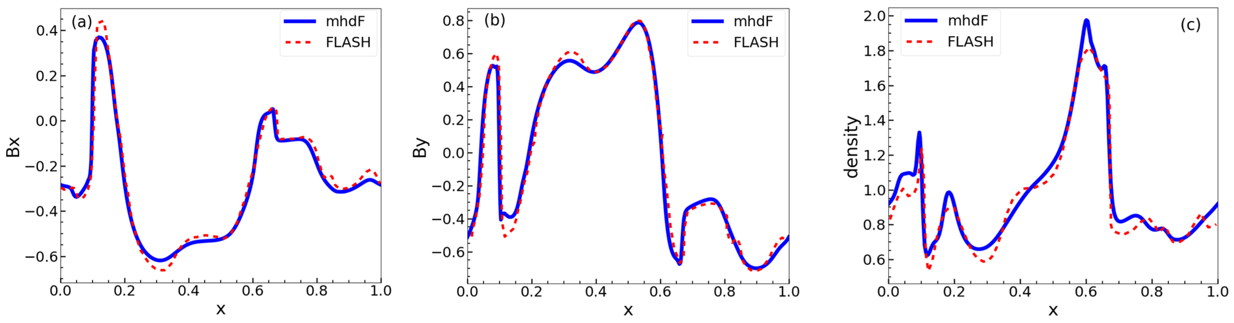
3.1.1. Orszag–Tang MHD Vortex Problem

Here, the classical Orszag–Tang MHD vortex problem is selected as a benchmark case to verify the mhdF solver. This case is a classic two-dimensional numerical test problem in MHD, widely used to verify the accuracy of MHD solvers and their ability to simulate the coupling effects between magnetic fields and fluid dynamics. It demonstrates the nonlinear interaction between magnetic fields and fluid motion, especially complex phenomena such as magnetic field stretching, compression, shock formation, and energy dissipation. This problem does not have an analytical solution but can be verified by comparing the results with those of other standard MHD solvers. After non-dimensionalization, the computational domain is $x, y\in {[0\hspace{0.33em}1]}^2$, and the initial conditions for magnetic flux density and velocity are as follows:

$$B_0=\left[-\sin (2\pi y),\hspace{0.33em}\sin (4\pi x)\right]/\gamma$$

(15)

$$U_0=\left[-\sin (2\pi y),\hspace{0.33em}\sin (2\pi x)\right]$$

(16)

where $\gamma =5/3$ is the adiabatic index; the initial values of pressure and density are $P_0=0.6$, ${\rho }_0=1.0$; and magnetic permeability is $\mu =1$. Here, we compare the results with those computed by the ideal MHD solver of the FLASH code [30]. The simulation results are as follows.

Figure 1 displays the distribution of magnitude of the magnetic flux density and density calculated by the mhdF solver at $t=0.4$. The results exhibit high structural consistency with those from the FLASH code [30], demonstrating identical complex vortex flow patterns.

Figure 2 compares the results calculated by the mhdF solver and the FLASH code at $t=0.4$ along the line $y=0.25$, showing the variations in the magnetic flux density components ($B_x$, $B_y$) and the density along the x-axis. The blue solid lines represent the results calculated by the mhdF solver, while the red dashed lines correspond to the results from the FLASH code. The overall computational results are largely consistent, with some discrepancies at peak values. The PIMPLE algorithm in the mhdF solver explicitly treats the pressure term, resulting in insufficient resolution for transonic shock discontinuities. In contrast, FLASH uses a high-order Godunov method, which better captures shock waves. Nevertheless, for supersonic problems, the calculation has already met the requirements for simulating the dynamic processes of CTs in the drift tube to a certain extent.

Here, the convergence order of the solver mhdF is discussed through relative errors. For the numerical results of the Orszag–Tang vortex simulation on an $N\times N$ grid at time $t$, the relative error of each variable is defined as follows:

$${\delta }_N(W)={\displaystyle \frac{{\displaystyle \mathbf{\sum }_{i=1}^N{\displaystyle \mathbf{\sum }_{k=1}^N\left|W_{i,k}^N-W_{i,k}^{\max }\right|}}}{{\displaystyle \mathbf{\sum }_{i=1}^N{\displaystyle \mathbf{\sum }_{k=1}^N\left|W_{i,k}^{\max }\right|}}}}$$

(17)

Here, $W_{i,k}^{\max }$ represents the simulated value at the coordinate $\left(i,k\right)$ on the high-resolution grid. The value of $\max$ is taken as 512. The combined relative error for multiple variables is defined as follows:

$${\delta }_N={\displaystyle \frac{1}{4}}\left({\delta }_N(U_x)+{\delta }_N(U_y)+{\delta }_N(B_x)+{\delta }_N(B_y)\right)$$

(18)

The corresponding formula for calculating the order of convergence is

$$R_N=-{\displaystyle \frac{\lg ({\delta }_N/{\delta }_{N_0})}{\lg (N/N_0)}}$$

(19)

Here, let $N_0=50$, which refers to the number of grid points in the coarsest grid, and $N_0<N$. The results at time $t=0.4$ show the distribution of relative errors and convergence orders for the two velocity components and the two magnetic field components, as illustrated in

Table 1. Relative errors and convergence orders of the velocity components and magnetic induction components for the Orszag–Tang MHD vortex problem.

$\mathit{N}$	${\mathit{\delta }}_{\mathit{N}}({\mathit{B}}_{\mathit{x}})$	${\mathit{\delta }}_{\mathit{N}}({\mathit{B}}_{\mathit{y}})$	${\mathit{\delta }}_{\mathit{N}}({\mathit{U}}_{\mathit{x}})$	${\mathit{\delta }}_{\mathit{N}}({\mathit{U}}_{\mathit{y}})$	${\mathit{\delta }}_{\mathit{N}}$	${\mathit{R}}_{\mathit{N}}$
50	0.19712	0.20513	0.23659	0.19642	0.20881	—
100	0.11271	0.11359	0.13713	0.10884	0.11807	0.82
200	0.05668	0.05661	0.06963	0.05531	0.05956	0.90
300	0.03443	0.03243	0.04792	0.03846	0.03831	0.95
400	0.01792	0.01764	0.02222	0.01736	0.01878	1.16

. It can be observed that as the grid resolution increases, the relative errors of each variable gradually decrease, and the convergence order of the mhdF solver falls within the range of 1 to 2. Although its convergence efficiency is lower than that of solvers using denser basis representations, it offers higher stability and demonstrates better fidelity in problems involving scattered optimization.

Through the simulation of the Orszag–Tang MHD vortex problem, the reliability of the mhdF solver in ideal magnetohydrodynamic scenarios has been systematically verified. This demonstrates that the program possesses engineering applicability in complex magnetic field coupling problems and meets the basic requirements for compact toroidal MHD simulations. In the following, another test case is used to verify the spatial convergence and temporal stability of the mhdF solver.

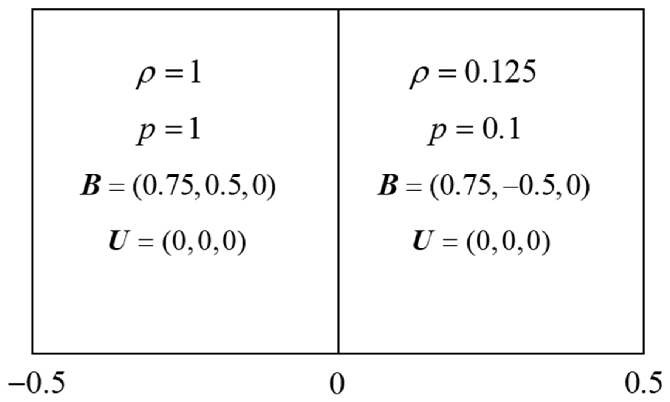
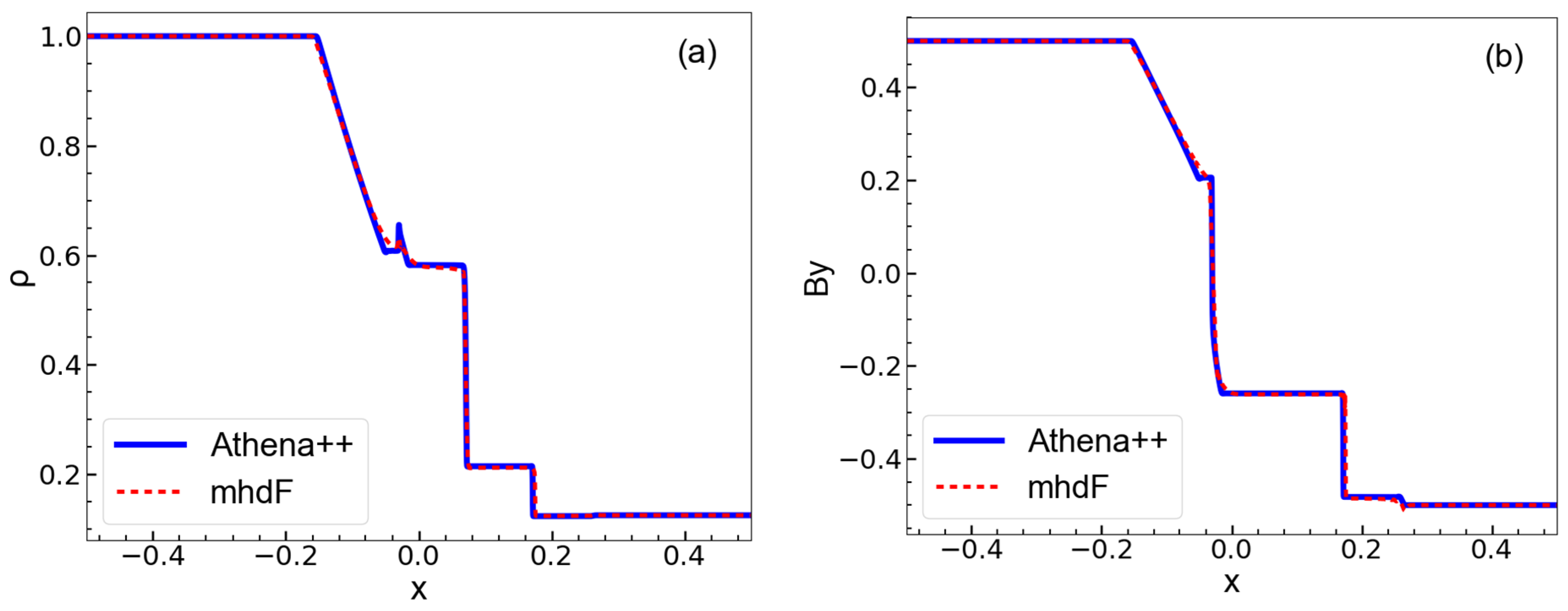
3.1.2. Brio–Wu Shock Tube Problem

The Brio–Wu shock tube problem is a classic one-dimensional benchmark test in magnetohydrodynamics (MHD) used to evaluate a solver’s ability to handle the interaction between magnetic fields and shock waves [31]. It was first proposed by Brio and Wu in 1988. After non-dimensionalization, the initial conditions are shown in Figure 3. At time $t=0$, the thin layer between the two regions ruptures, and the gases on either side interact to form a system of shock waves in the center of the tube. Due to the limited capability of the mhdF solver in handling shock problems, a modification was made to the original initial conditions: the magnetic field was reduced from 1 to 0.5. Figure 4 shows the simulation results at time t from both the mhdF solver and the Roe solver implemented in the Athena++ code. It can be seen that the results for the magnetic field component $B_y$ and the density $\rho$ produced by the two solvers are largely consistent.

The following section analyzes the Brio–Wu shock tube problem to examine the temporal stability and spatial convergence of the mhdF solver. The relative numerical error in density is defined as follows:

$${\delta }_N(\rho )={\displaystyle \frac{{\displaystyle \sum _{i=1}^N\left|{\rho }_i^N-{\rho }_i^{\mathrm{exact}}\right|}}{{\displaystyle \sum _{i=1}^N\left|{\rho }_i^{\mathrm{exact}}\right|}}}$$

(20)

Here, ${\rho }_i^{\mathrm{exact}}$ refers to the density value at position $x_i$ computed by the Roe solver in the Athena++ code with a grid resolution of $N=3072$, which is treated as the reference solution. The relative errors in density computed by the mhdF solver under grid resolutions of $N=500,1000,2000$ are then evaluated, and the results are shown in Figure 5. For all simulations—including both the Athena++ Roe solver and the mhdF solver—the one-dimensional Courant number $Co\equiv U_{\max }\Delta t/\Delta x$ is kept below 0.2. Here, $\Delta t$ denotes the time step size and $\Delta x$ the spatial grid spacing. The results show that the error produced by the mhdF solver does not exhibit abrupt changes over time and remains relatively stable, indicating good temporal stability. Moreover, as the number of grid points increases, the error decreases significantly, and the fluctuation in the error over time is also suppressed to a certain extent. This demonstrates that the mhdF solver has good spatial convergence properties.

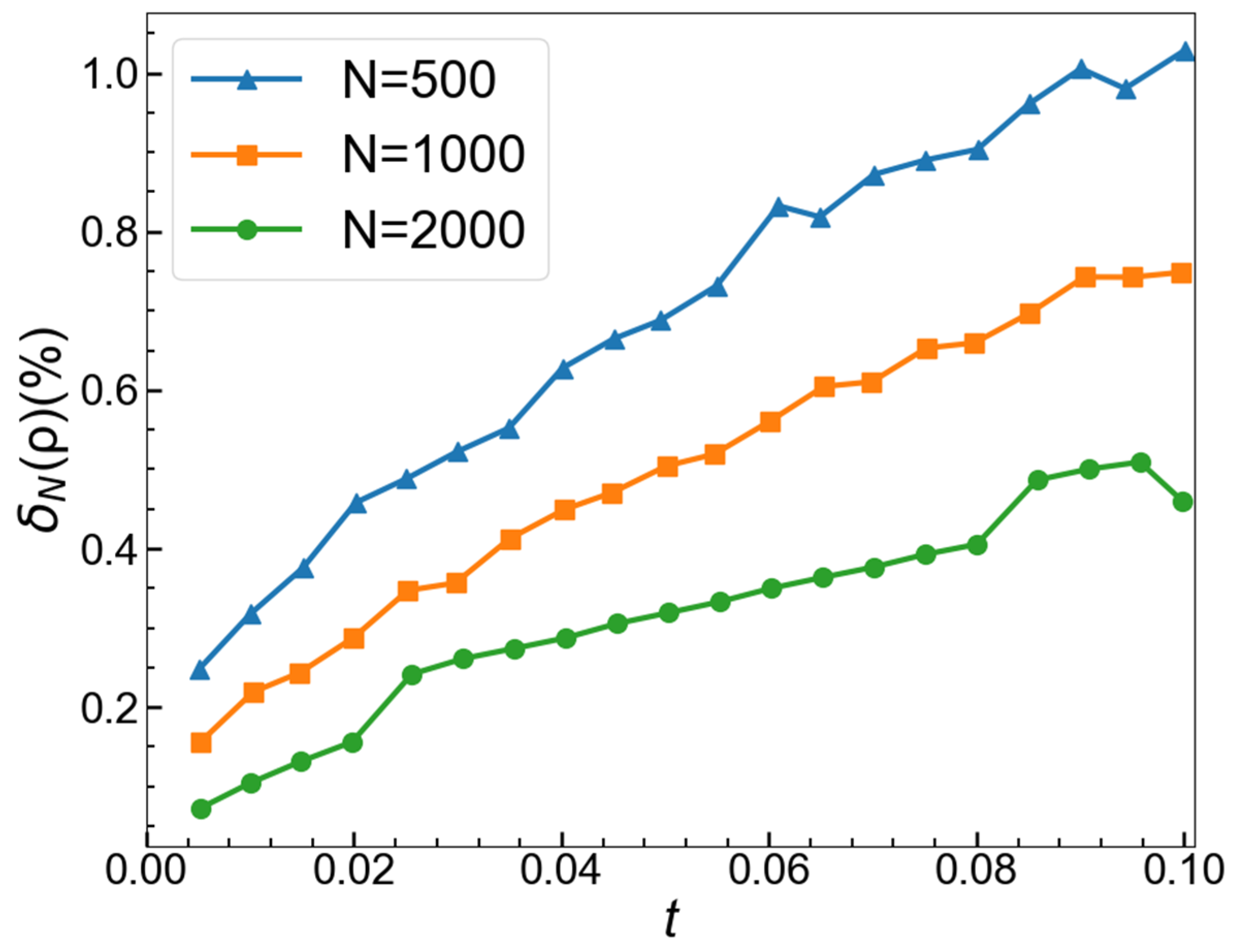
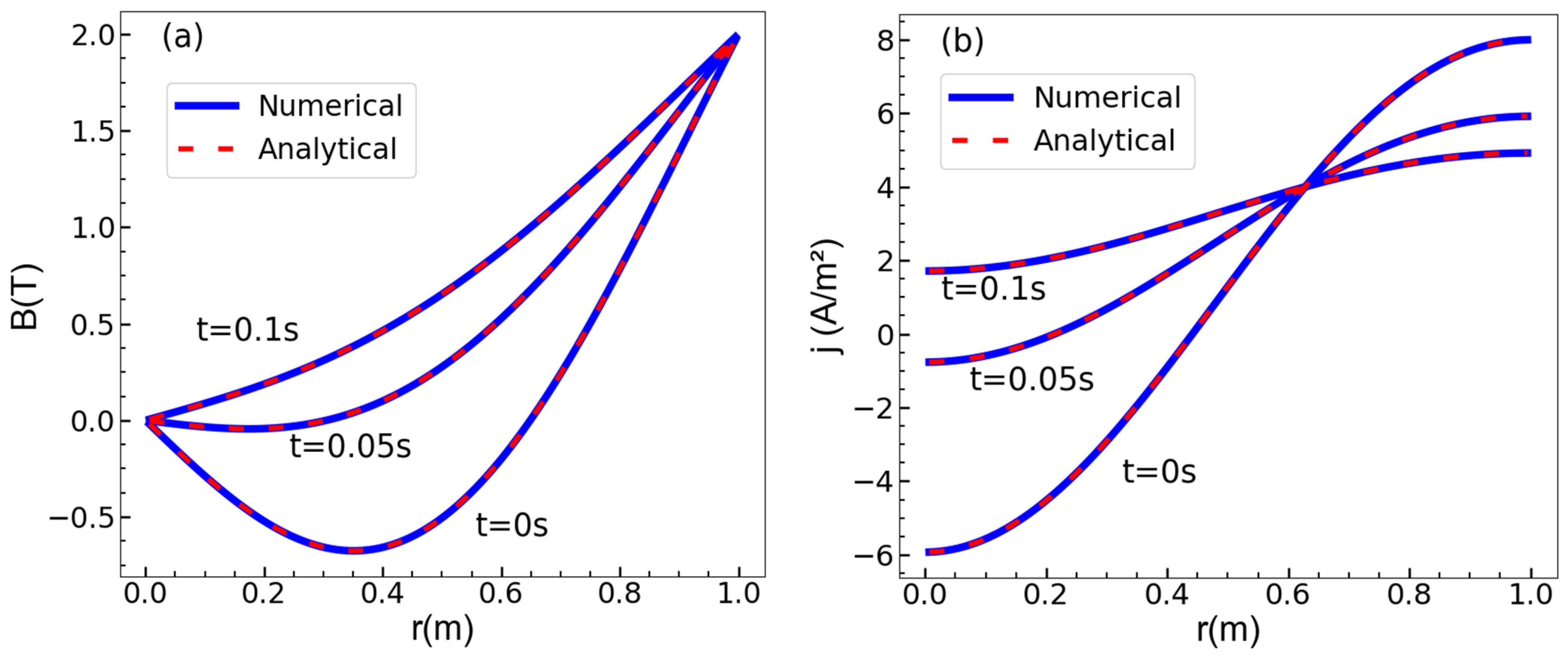
3.2. Magnetic Diffusion Solver Verification

To verify the accuracy of the magnetic diffusion solver, this study selects the conductive cylinder model with analytical solutions proposed by Miller [32] for numerical testing. This model considers an axisymmetric 2D cylindrical conductor, where the current source is applied axially, and the magnetic field is distributed only in the azimuthal direction and is a function of radius $r$ and time $t$, assuming the electrical conductivity $\sigma$ is a spatially uniform constant and both ends of the cylinder apply zero normal flux boundary conditions. If the total current is $S(t)$, the magnetic field at the surface of the cylindrical conductor can be calculated using the integral form of Ampère’s law:

$$B{(r,t)}_{\mathrm{exterior}}={\displaystyle \frac{2S(t)}{r}}$$

(21)

When the total current is a constant $S(t)=S_0$, the analytical solutions for magnetic flux density and current density are

$$B(r,t)={\displaystyle \frac{2r{S}_0}{R_w^2}}\left[1+2{\displaystyle \sum _{n=1}^{\infty }\frac{R_w}{r{y}_n}}{\displaystyle \frac{J_1\left(\frac{r}{R_w}{y}_n\right)}{J_0(y_n)}}{e}^{-t{\displaystyle \frac{y_n^2}{b^2}}}\right]$$

(22)

$$j(r,t)={\displaystyle \frac{S_0}{\pi R_w^2}}\left[1+{\displaystyle \sum _{n=1}^{\infty }\frac{J_0\left(\frac{r}{R_w}{y}_n\right)}{J_0(y_n)}}{e}^{-t{\displaystyle \frac{y_n^2}{b^2}}}\right]$$

(23)

where $b=R_w\sqrt{{\mu }_0\sigma }$ and $y_n$ are the n-th non-zero roots of $J_1\left(y\right)=0$.

Numerical simulation parameters are set as follows: total current $S_0=1.0\mathit{A}$, cylinder radius $R_w=1.0\mathrm{m}$, vacuum permeability ${\mu }_0=1.256\times {10}^{-6}{\mathrm{N}/\mathrm{A}}^2$, electrical conductivity $\sigma =1.0\mathrm{S}/\mathrm{m}$. The initial value of magnetic flux density is

$$B(r,0)={\displaystyle \frac{2r{S}_0}{R_w^2}}\left[1+2{\displaystyle \frac{R_w}{r{y}_1}}{\displaystyle \frac{J_1\left(\frac{r}{R_w}{y}_1\right)}{J_0(y_1)}}\right]$$

(24)

The magnetic diffusion solver is used to compute and compare the numerical solution with the analytical solution at $t=0, 0.05, 0.1 \mathrm{s}$. As shown in Figure 6, the blue solid lines represent the numerical solutions, and the red dashed lines denote the analytical solutions. The numerical and analytical solutions match closely in the distribution of magnetic flux density and current density, indicating that the magnetic diffusion solver can accurately capture the dynamic process of magnetic field diffusion.

3.3. The mhdMRF Solver Verification

To verify the mhdMRF solver, based on the validations of the two individual solvers above, this study designs a one-dimensional analytical example to verify the correctness of the interface coupling boundary conditions. This model assumes a very small velocity field, so that magnetic field evolution in the fluid region approximately follows the magnetic diffusion equation. Then, the governing equation in both regions simplifies to

$${\displaystyle \frac{\partial B(x,t)}{\partial t}}={\displaystyle \frac{\partial }{\partial x}}\left[{\eta }_m{\displaystyle \frac{\partial B(x,t)}{\partial x}}\right]$$

(25)

where ${\eta }_m=1/\mu \sigma$ is the magnetic diffusion coefficients. The computational domain is defined as $x\in [-L,L]$, with the material interface at $x=0$, and the electrical conductivities in the solid region $x\in [-L,0]$ and fluid region $x\in [0,L]$ are as follows:

$$\sigma (x)=\left\{\begin{array}{cc}{\sigma }_1,\hfill & x\in [-L,0],\hfill \\ {\sigma }_2,\hfill & x\in [0,L],\hfill \end{array}\right.$$

(26)

Boundary conditions:

$$B(-L,t)=0, B(L,t)=0$$

(27)

At the interface, continuity of field and flux must be satisfied:

$$B(0^{-},t)=B(0^{+},t)$$

(28)

$${\eta }_{m1}{\displaystyle \frac{dB(0^{-},t)}{dx}}={\eta }_{m2}{\displaystyle \frac{dB(0^{+},t)}{dx}}$$

(29)

Using the method of separation of variables, the analytical solution can be expressed as an eigenfunction expansion:

$$B(x,t)={\displaystyle \sum _{n=1}^{\infty }{a}_n}{X}_n(x)e^{-{\lambda }_{n}t}$$

(30)

The eigenfunction $X_n(x)$ is expressed in the solid and fluid regions as

$$X_n(x)=\left\{\begin{array}{ll}{A}_n\sin \left[k_{1,n}(x+L)\right],\hfill & x\in [-L,0]\hfill \\ C_n\sin \left[k_{2,n}(L-x)\right],\hfill & x\in [0,L]\hfill \end{array}\right.$$

(31)

where $k_{1,n}=\sqrt{{\lambda }_n/{\eta }_{m1}}$, $k_{2,n}=\sqrt{{\lambda }_n/{\eta }_{m2}}$, and coefficients $A_n$, $C_n$ are determined by interface matching conditions:

$$A_n\sin (k_{1,n}L)=C_n\sin (k_{2,n}L)$$

(32)

The eigenvalue ${\lambda }_n$ is determined by the transcendental equation:

$${\displaystyle \frac{\sin (k_{1,n}L)}{\sin (k_{2,n}L)}}=-\sqrt{{\displaystyle \frac{{\eta }_{m1}}{{\eta }_{m2}}}}{\displaystyle \frac{\cos (k_{1,n}L)}{\cos (k_{2,n}L)}}$$

(33)

The first eigenvalue is ${\lambda }_1\approx 0.771$. Simulation parameters: $L=1$, $\mu =1$, ${\sigma }_1=10$, ${\sigma }_2=1$. Initial condition:

$$B(x,0)=X(x)=\left\{\begin{array}{ll}A\sin \left[k_1(x+L)\right],\hfill & x\in [-L,0]\hfill \\ C\sin \left[k_2(L-x)\right],\hfill & x\in [0,L]\hfill \end{array}\right.$$

(34)

Taking $C=0.1$, we find $A\approx 0.216$ based on matching conditions. Other variables in the fluid region are set to small values to avoid interfering with magnetic field evolution.

Figure 7 compares analytical and numerical solutions at $t=0.4, 0.8, 1.2$; the blue solid line represents the numerical solution calculated by the solver, while the red dashed line corresponds to the analytical solution. The results show high spatial agreement. The relative error of magnetic induction is defined as follows:

$${\delta }_N(B)={\displaystyle \frac{{\displaystyle \sum _{i=1}^N\left|B_i^{anl}-B_i^{n\mathit{U}m}\right|}}{{\displaystyle \sum _{i=1}^N\left|B_i^{anl}\right|}}}$$

(35)

The error at each time point is approximately ${\delta }_N(B)\approx 1\times {10}^{-4}$. The continuity of field and flux is correctly implemented through the custom interface coupling boundary condition. This shows that the mhdMRF solver can accurately handle the dynamic matching of magnetic fields and fluxes at interfaces.

Figure 7. Comparing the analytical and numerical solutions for the validation case of the mhdMRF solver.

Figure 7. Comparing the analytical and numerical solutions for the validation case of the mhdMRF solver.

4. Numerical Simulation of CT Magnetohydrodynamics

This section aims to conduct numerical simulation of the motion process of CTs in drift tubes using the developed mhdF solver and mhdMRF solver, focusing on the influence of the inner electrode end geometry and finite resistivity wall on the magnetic field distribution and overall dynamic characteristics.

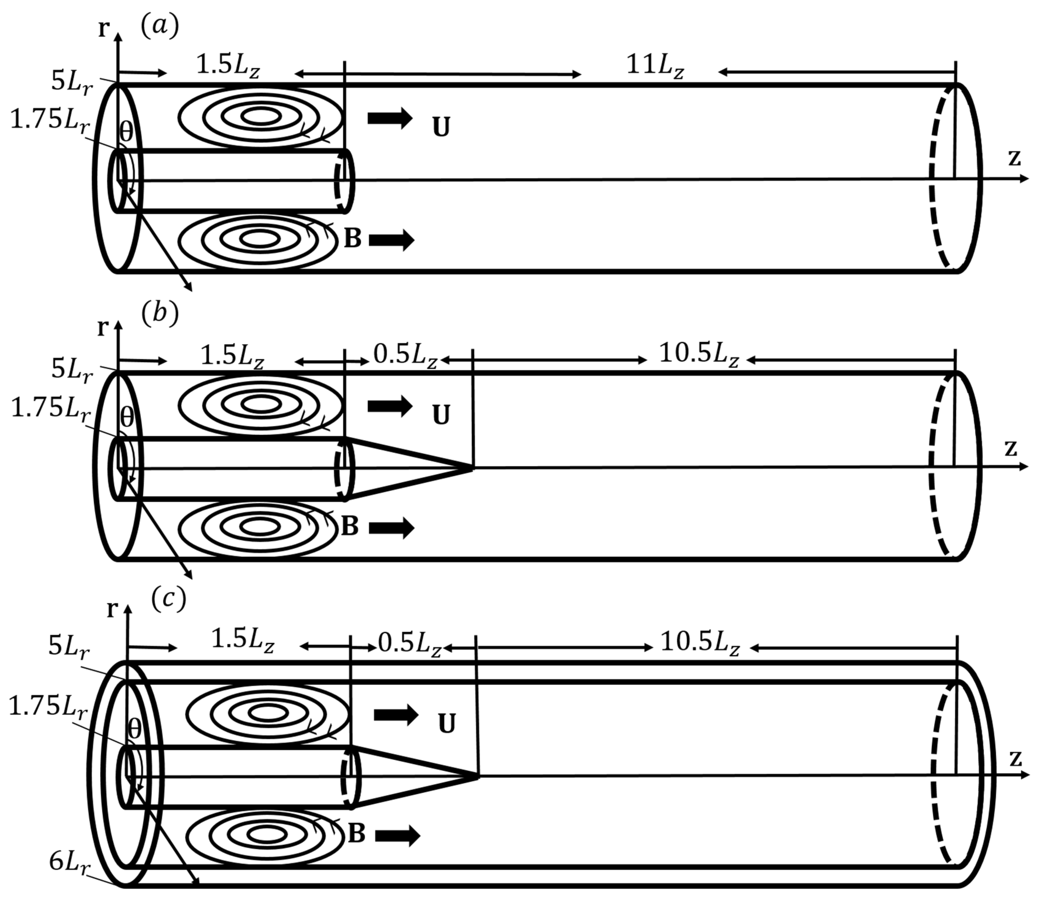
4.1. Geometric Structure and Simulation Parameter Settings

In the CT injection device, the acceleration region adopts a cylindrical metal conductor as the inner electrode. To investigate the influence of the inner electrode end geometry on the MHD behavior of the CT, this paper innovatively introduces a conical transition section at the end of the cylinder. To systematically study this problem and simultaneously consider the effect of the finite resistive wall, four typical cases are designed. The simulation domains can be categorized into three types, as shown in Figure 8.

• Case 1: the internal metal electrode is a pure cylinder (hereinafter referred to as the cylindrical inner electrode);
• Case 2: a conical transition section is added to the end of the cylinder (hereinafter referred to as the conical inner electrode);
• Cases 3 and 4: based on the geometry of Case 2, an outer finite resistivity wall region is added, with different wall resistivity values in each case.

In terms of simulation parameters, the inner electrode radius, $r_{in}=1.75L_r$, and the outer radius from the central axis to the wall, $r_{out}=5L_r$, are based on the EAST-CTI device parameters [15], where $L_r=0.01 \mathrm{m}$ and the axial length $L_z=0.1 \mathrm{m}$. The initial magnetic field distribution of the CT is calculated using the analytical solution by Degnan [33] under perfectly conducting wall conditions. The magnetic field is distributed within the region of inner radius $1.75L_r$, outer radius $5L_r$, and axial length $L_z$, that is, the region from $z=-0.2 \mathrm{m}$ to $z=-0.1 \mathrm{m}$, and the characteristic value is set as the minimum value. The initial magnetic field in other regions is zero. The initial density of the CT is given by the poloidal flux function ${\psi }_{pol}=r{A}_{\theta }$, satisfying the following expression [21]:

$$\rho ={\rho }_{\min }+({\rho }_{\max }-{\rho }_{\min }){\displaystyle \frac{\left|{\psi }_{\mathrm{pol}}\right|}{\left|{\psi }_{\mathrm{axis}}\right|}}$$

(36)

Here, the peak density and background plasma density of the CT are ${\rho }_{\max }=2\times {10}^{-5} \mathrm{kg}/{\mathrm{m}}^3$ (corresponding to $n_{CT}={10}^{22} {\mathrm{m}}^{-3}$) and ${\rho }_{\min }=2\times {10}^{-7} \mathrm{kg}/{\mathrm{m}}^3$, respectively, and ${\psi }_{\mathrm{axis}}$ is the poloidal flux at the axis. The background density equals 1% of the peak density of the CT. Experimentally measured CT temperatures typically range within $1 \mathrm{eV}–10 \mathrm{eV}$. Here, the initial temperature at the location of the maximum CT density is taken as $5 \mathrm{eV}$. The initial pressure across the entire domain is kept equal, calculated via the ideal gas equation of state, yielding approximately $2.4\times {10}^3 \mathrm{Pa}$. The initial velocity of the CT and other regions is set to a typical experimental value of $100 \mathrm{km}/\mathrm{s}$, in the positive z-direction. Magnetic permeability is set to vacuum permeability, dynamic viscosity is $\mu =0.001 \mathrm{kg}/(\mathrm{m}·\mathrm{s})$, and thermal conductivity is $\kappa =1\mathrm{w}/(\mathrm{m}·\mathrm{K})$. The resistivity of the CT is estimated using the Spitzer resistivity formula as ${\eta }_{CT}=1\times {10}^{-5} \mathsf{\Omega }·\mathrm{m}$, and the finite resistive wall resistivity in Cases 3 and 4 are set as ${\eta }_w=1\times {10}^{-7} \mathsf{\Omega }·\mathrm{m}$ and ${\eta }_w=1\times {10}^{-5} \mathsf{\Omega }·\mathrm{m}$, respectively.

In Cases 1 and 2, the surfaces of the inner electrode and the outer wall use zero-gradient conditions for temperature and pressure and perfectly conducting wall conditions for magnetic flux density. Since viscous effects are largely neglected in the simulation, slip boundary conditions are used for velocity at the wall. In Cases 3 and 4, the inner surface of the finite resistive wall is set to zero-gradient conditions for temperature and pressure and slip conditions for velocity, and the magnetic flux density uses the custom internal coupling boundary condition mentioned in Section 2. The outer surface of the finite conductive wall is set to fixed zero magnetic field. Moreover, since the CT satisfies toroidal symmetry, all four cases adopt OpenFOAM’s built-in wedge boundary condition (for solving axisymmetric problems), reducing the 3D problem to 2D r-z plane simulation. The maximum grid size is $4\mathrm{mm}$.

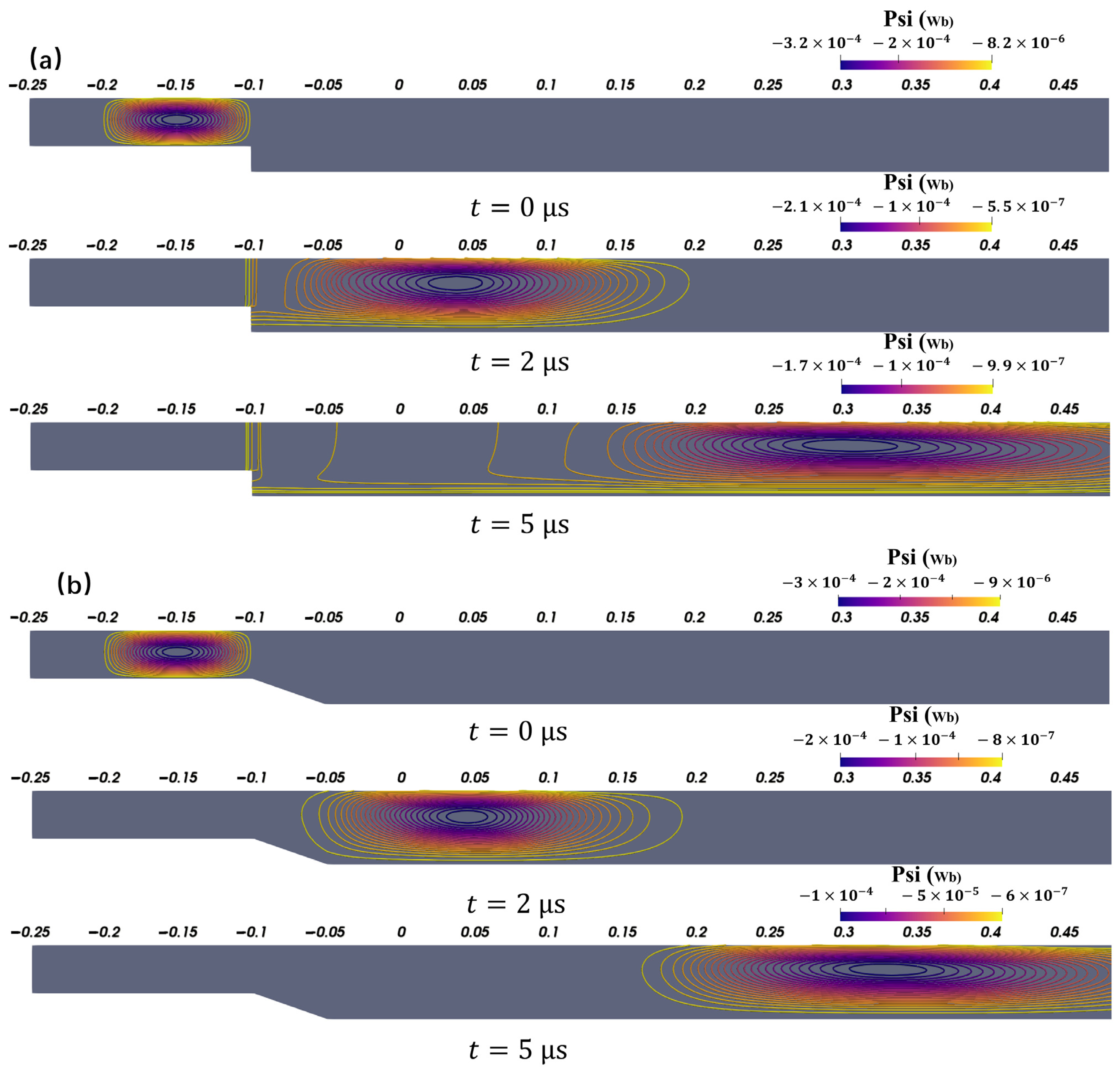
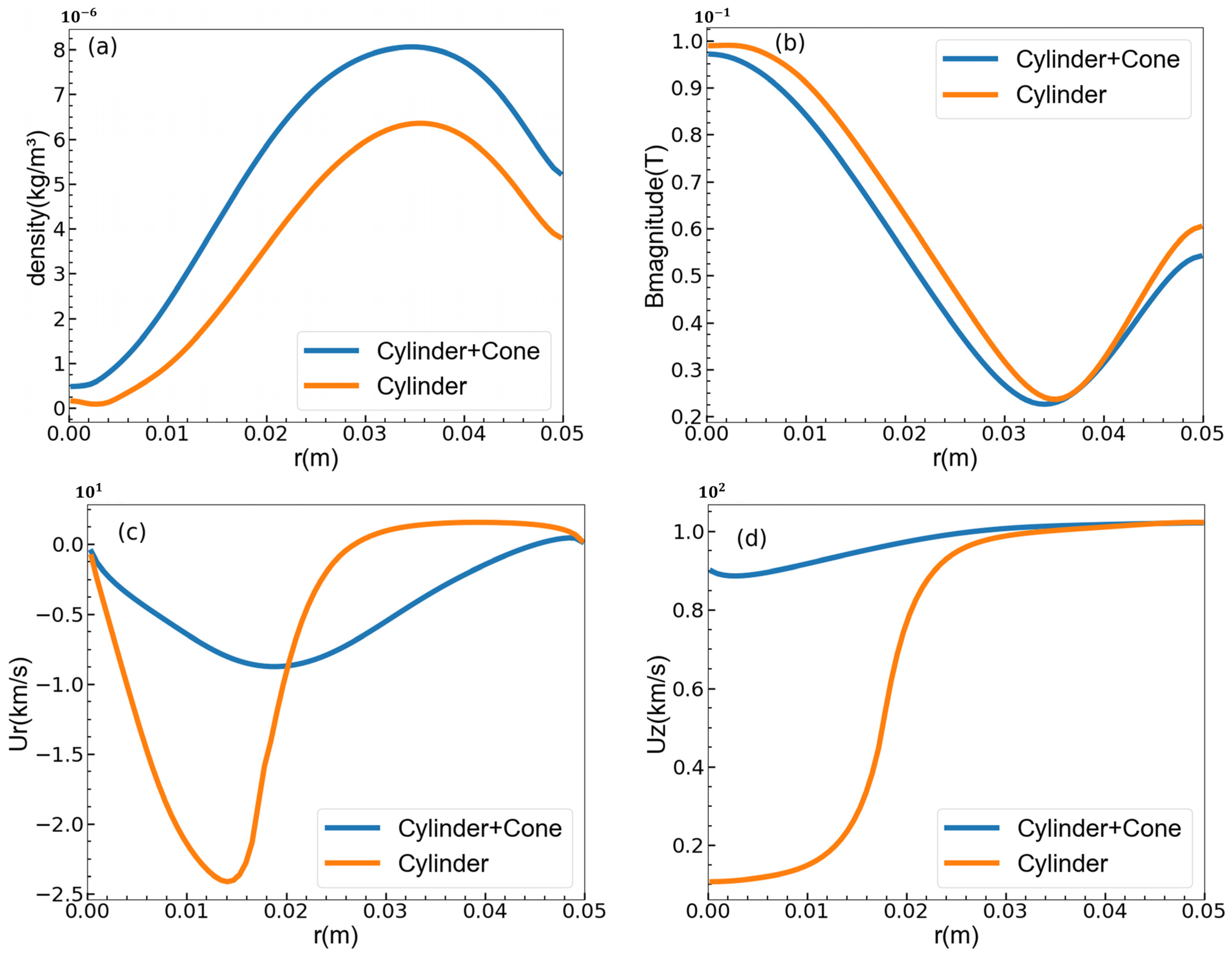
4.2. Influence of Inner Electrode End Geometry on CTs

By comparing the simulation results of the cylindrical inner electrode and the conical inner electrode, significant differences in the magnetic field evolution of the compact toroid under the two structures can be observed. Figure 9a,b, respectively, show the distributions of poloidal magnetic flux at time $t=0, 2, 5 \mathsf{\mu }\mathrm{s}$ in the two cases. The definition of poloidal magnetic flux is

$${\psi }_{\mathit{pol}}=\int B_z·d{S}_p$$

(37)

where $S_p$ is a circular area with radius $r$ starting from the z-axis. The color shade reflects the magnitude of the magnetic flux. The scale above represents the coordinate along the z-axis in meters. The results show that in the case of the cylindrical inner electrode, the originally closed magnetic field structure near the end region of the inner electrode (located near the z-axis) is disrupted, and the outer magnetic field is stretched in the negative z-direction. In contrast, under the conical inner electrode structure, the magnetic field structure is better preserved, and the overall distribution is more complete.

In addition, Figure 10a,b show the distribution of density and magnetic flux density magnitude along the radial direction (r-direction) near the CT density peak (located at $z=0.305 \mathrm{m}$ for Case 1 and $z=0.335 \mathrm{m}$ for Case 2) at time $t=5 \mathsf{\mu }\mathrm{s}$. The comparison clearly shows that under the conical inner electrode configuration, the density peak is steeper and more concentrated (the maximum density for the cylindrical inner electrode is approximately $6.4\times {10}^{-5} {\mathrm{kg}/\mathrm{m}}^3$, and that for the conical inner electrode is approximately $8.1\times {10}^{-5} {\mathrm{kg}/\mathrm{m}}^3$), indicating that the introduction of the transition region improves the confinement effect of the CT. Meanwhile, in the area near the z-axis, the magnetic field strength under the cylindrical inner electrode is generally slightly higher, which is likely caused by velocity non-uniformity.

Based on the spatial distribution of velocity, Figure 10c,d compare the velocity components in the radial direction, including the radial component $U_r$ and the axial component $U_z$. Figure 10c displays results for Case 1 at $t=0.5 \mathsf{\mu }\mathrm{s}$, $z=-0.1 \mathrm{m}$; Figure 10d displays results for Case 2 at $t=1 \mathsf{\mu }\mathrm{s}$, $z=-0.05 \mathrm{m}$. (Here, the z-coordinates indicate locations where velocity variations are most pronounced, and the times correspond to moments when the compact torus traverses these positions.) A considerable variation in velocity is observed in the region $0 \mathrm{m}\le r\le 0.03 \mathrm{m}$ under the configuration of a cylindrical inner electrode. In the case of the conical inner electrode, the presence of a transitional region effectively reduces the velocity gradient in the corresponding area, resulting in a smoother propagation process of the CT.

This indicates that the geometric structure at the end of the inner electrode has a significant influence on the motion of the CT within the drift tube. In addition to serving as an accelerating component in the acceleration zone, the inner electrode also acts as a perfectly conducting wall, providing effective confinement for the CT. However, for a cylindrical inner electrode, this confinement effect abruptly disappears at the electrode’s terminal point, where the original wall boundary is suddenly replaced by a free boundary, leading to rapid changes in both magnetic field and velocity in that region. By incorporating a conical transition section at the end of a cylindrical inner electrode, the velocity variation can be effectively mitigated, thereby facilitating stable transport of the CT. Moreover, this structural modification significantly enhances the confinement capability and better preserves the integrity of the magnetic field configuration.

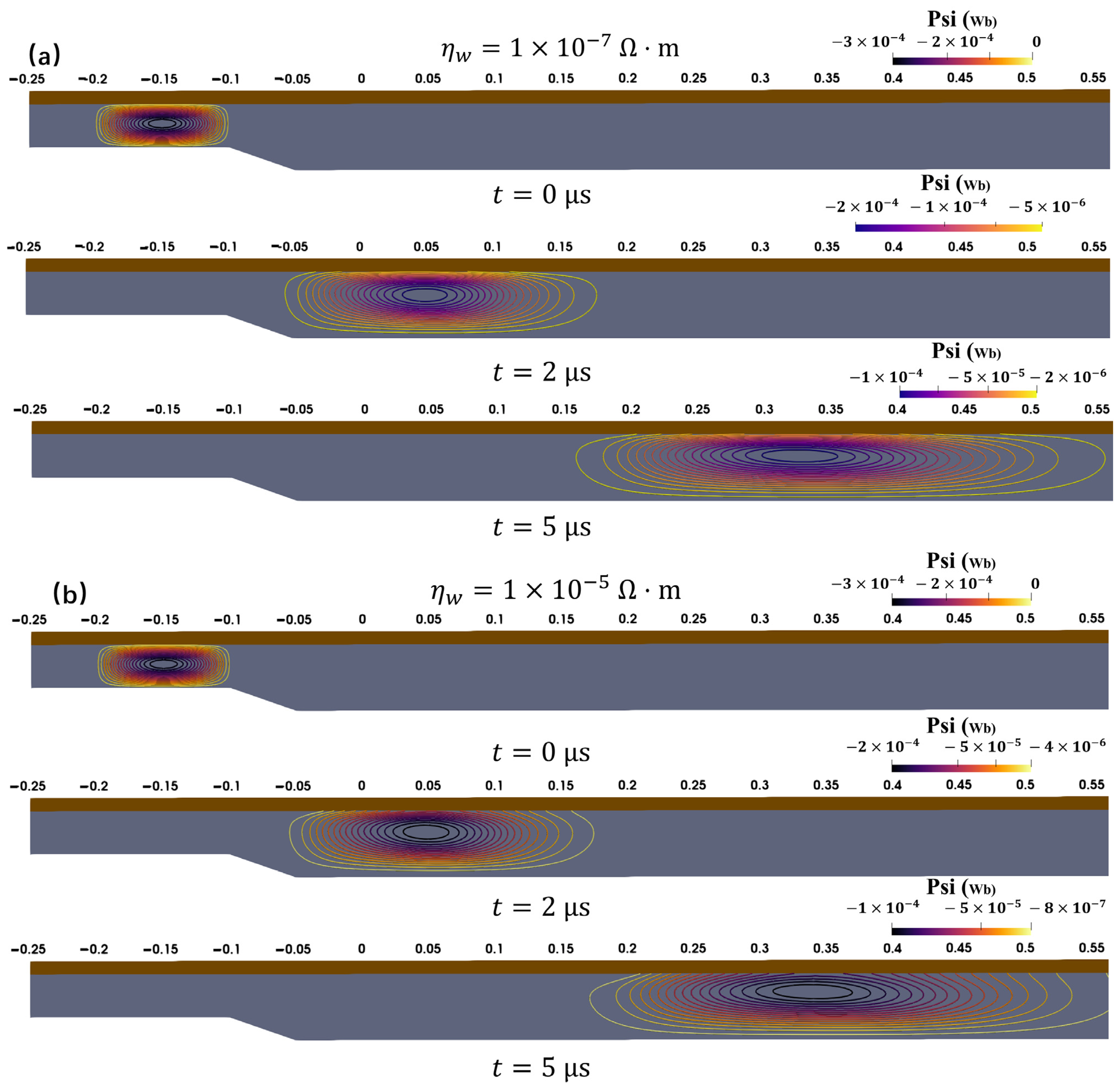
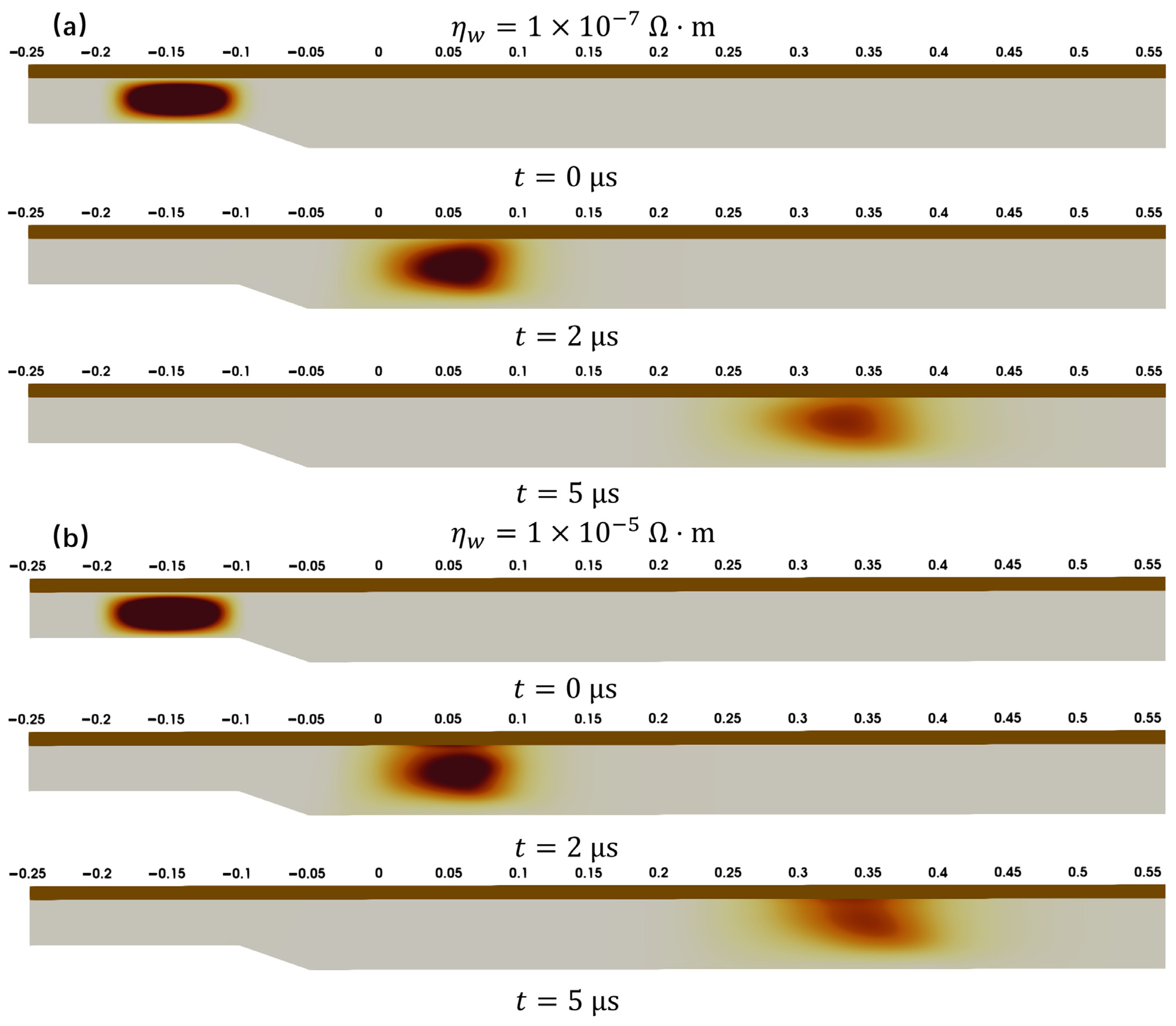
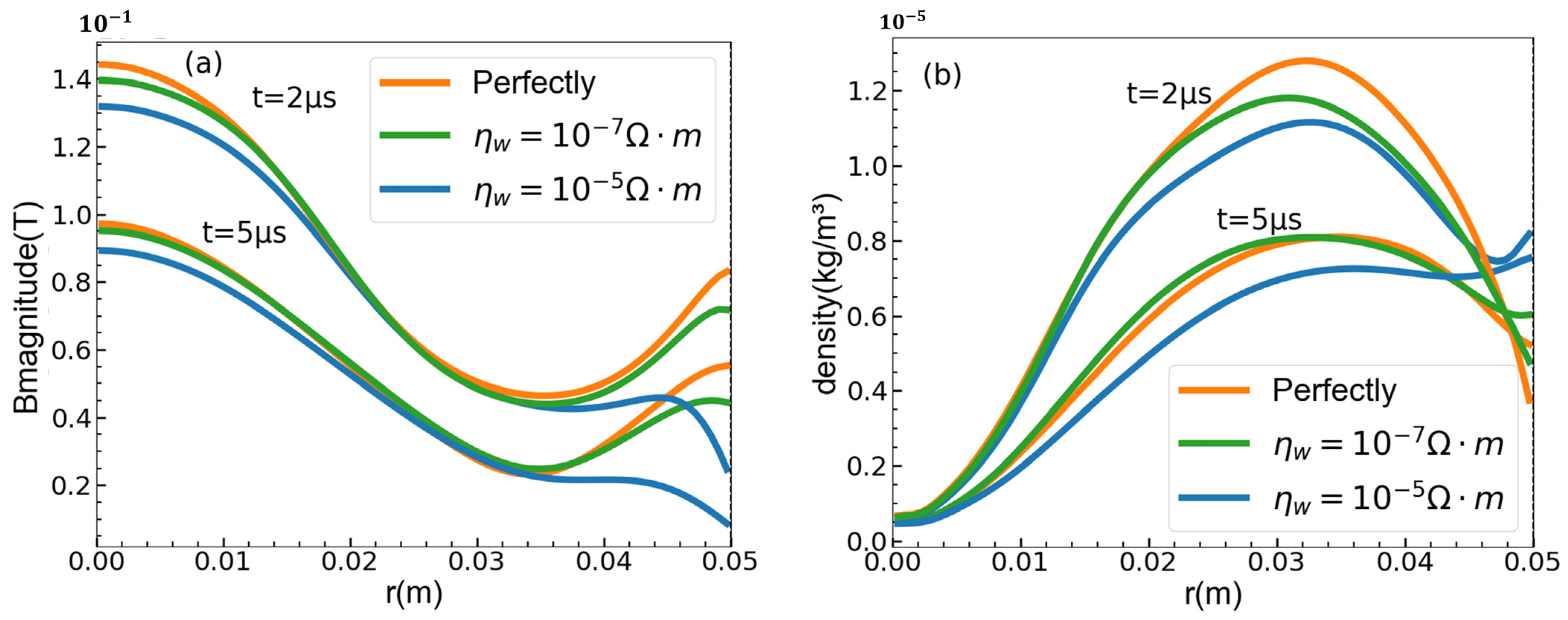
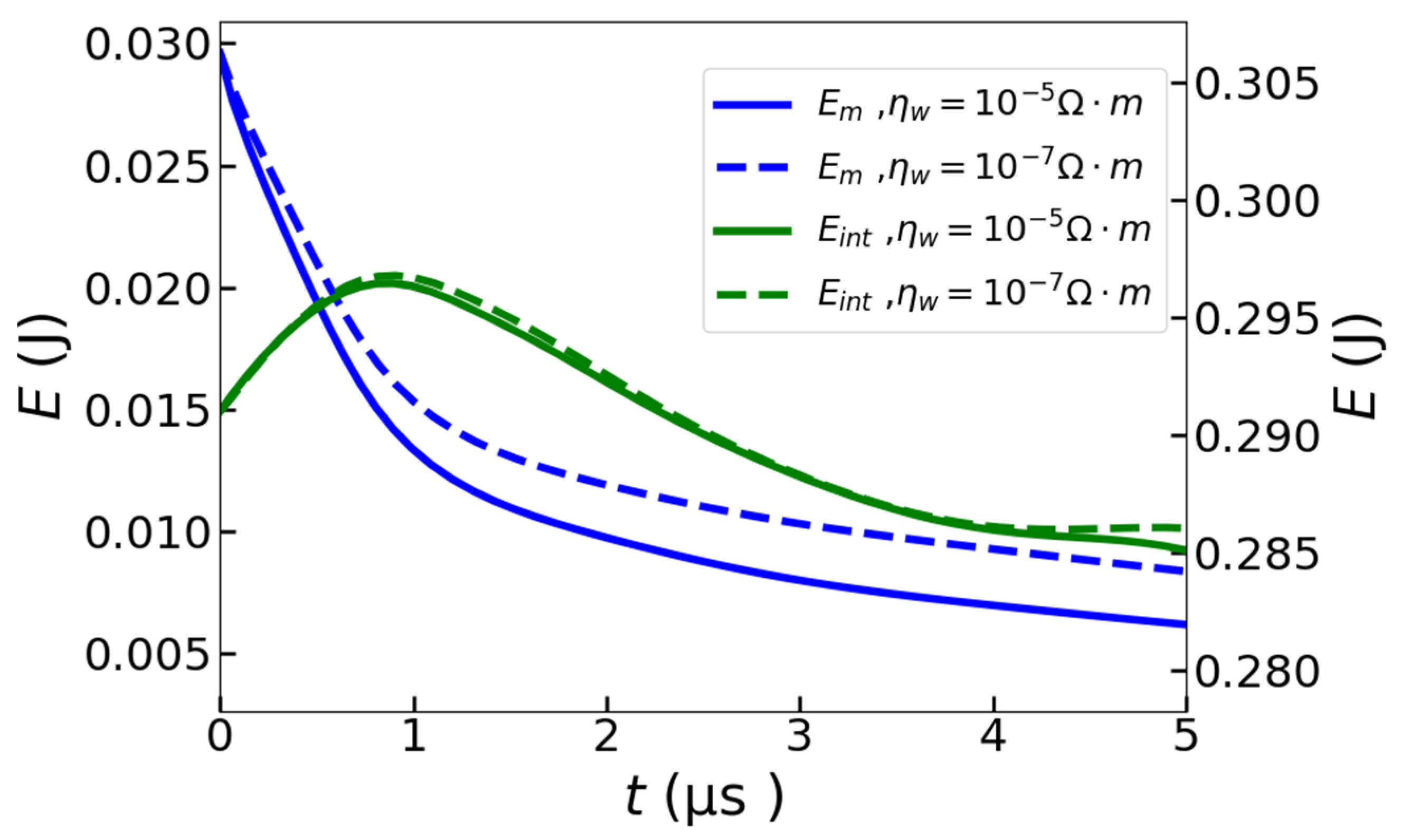
4.3. Influence of Finite-Resistivity Walls on CTs

Cases 3 and 4 are solved using the mhdMRF solver. Figure 11a,b show the distributions of poloidal magnetic flux at $t=0, 2, 5 \mathsf{\mu }\mathrm{s}$ for the two cases with different resistivities of the finite resistivity wall: ${\eta }_w=1\times {10}^{-7} \mathsf{\Omega }·\mathrm{m}$ (small resistivity) and ${\eta }_w=1\times {10}^{-5} \mathsf{\Omega }·\mathrm{m}$ (large resistivity), respectively. The depth of color reflects the magnitude of the poloidal magnetic flux, while the closure of contour lines indicates the integrity of the magnetic field structure. By observing Figure 11a,b, it is evident that closed magnetic field structures near the wall surfaces gradually disappear over time. In the case of small wall resistivity, the magnetic field structure is more complete compared with the large-resistivity case. The poloidal magnetic flux values are also larger in the lower resistivity case. This is because the higher the wall resistivity, the faster the magnetic field of the CT diffuses into the wall and the more the magnetic structure at the wall surface is affected.

Figure 12a,b compare the spatial density distributions of two cases at $t=0, 2, 5 \mathsf{\mu }\mathrm{s}$. Darker colors indicate higher densities, which also reflect the confinement effectiveness. In this study, the density evolution is primarily driven by the diffusion effects of the CT itself, as thermal conduction effects of the plasma are included. However, compared with the lower-resistivity case, the density distribution in the higher-resistivity case shows a significant shift toward the finite-resistivity walls. At $t=2,5 \mathsf{\mu }\mathrm{s}$, the darker colors near the walls in Figure 12b compared with Figure 12a suggest enhanced particle accumulation in the vicinity of the walls under higher resistivity conditions.

By comparing the radial distributions of physical quantities under different conditions, the influence of finite-resistivity walls on the CT can be visualized more directly. Figure 13 presents the radial distributions of magnetic flux density magnitude and density at $t=2, 5 \mathsf{\mu }\mathrm{s}$ under three configurations: perfectly conducting wall (Case 2) and finite-resistivity walls with resistivity values of $1\times {10}^{-7} \mathsf{\Omega }·\mathrm{m}$ and $1\times {10}^{-5} \mathsf{\Omega }·\mathrm{m}$. The z-coordinates selected correspond to the locations where the magnetic flux density magnitude or density reaches its maximum value. The influence of finite-resistivity walls on the CT magnetic field exhibits regional variations in the radial direction. The influence of wall resistivity on the magnetic field is primarily concentrated within the range of $0.036 \mathrm{m}\le r\le 0.05 \mathrm{m}$. In contrast, within the core region $0 \mathrm{m}\le r\le 0.012 \mathrm{m}$, the effect is minimal, with virtually no observable difference in the central region. Under the large-resistivity case, there is obvious density accumulation near the wall, and the peak density is relatively low. In contrast, in the small-resistivity case and the perfectly conducting wall case, the density distribution remains well peaked.

This type of radial transport of density is likely caused by differences in magnetic field diffusion rates at the wall surface when the compact torus interacts with the boundary. The boundary conditions for a compact torus forming a force-free magnetic field configuration differ from those in the drift tube. As a result, when the compact torus moves into the drift tube, its original force-free magnetic configuration gradually decays, leading to the emergence of Lorentz forces. The higher the resistivity of the conducting wall, the faster the force-free magnetic configuration of the compact torus deteriorates, resulting in differences in its radial transport behavior. Figure 14 examines the time evolution of magnetic energy $E_m={\displaystyle \int \frac{B^2}{2{\mu }_0}dV}$ and internal energy $E_{int}={\displaystyle \int \rho C_{v}TdV}$ for two simulation cases, where $V$ denotes the volume of the computational domain. The blue line represents magnetic energy, the green line represents internal energy, solid lines correspond to a resistivity of $1\times {10}^{-5} \mathsf{\Omega }·\mathrm{m}$, and dashed lines correspond to a resistivity of $1\times {10}^{-7} \mathsf{\Omega }·\mathrm{m}$. The change in internal energy shows little difference between the two resistivity cases; however, the internal energy is slightly higher when the resistivity is lower. This is because magnetic field dissipation at the boundary occurs more slowly, allowing more magnetic energy to be converted into internal energy via Ohmic dissipation. In contrast, there is a significant difference in magnetic energy dissipation. With a resistivity of $1\times {10}^{-5} \mathsf{\Omega }·\mathrm{m}$, the magnetic energy drops to one-third of its initial value after approximately $1.8 \mathsf{\mu }\mathrm{s}$, while with a resistivity of $1\times {10}^{-7} \mathsf{\Omega }·\mathrm{m}$, it takes about $3.6 \mathsf{\mu }\mathrm{s}$ to reach the same level—a difference of nearly a factor of two in time.

5. Conclusions

This study developed a compressible MHD solver, mhdF, and a magnetic diffusion solver on the OpenFOAM platform. These solvers are integrated into a multi-region coupling framework to create a multi-region coupled compressible MHD solver, mhdMRF, aimed at investigating the dynamic processes of CT in drift tubes and the influence of finite-resistivity walls. The solvers’ accuracy and engineering applicability in addressing MHD and magnetic diffusion problems were validated. By implementing custom interface coupling boundary conditions, the magnetic field coupling between fluid regions and finite-resistivity wall regions was achieved. The research further explored the effects of the geometric structure of the inner electrode tip and finite-resistivity walls on the MHD behavior of the CT. Numerical results demonstrate that during the transition of the CT from the acceleration zone to the drift tube, the geometric structure of the inner electrode tip plays a critical role in regulating the distributions of the magnetic and flow fields. Introducing a conical transition section to the traditional cylindrical inner electrode significantly reduces local velocity gradients, enhances magnetic field structural integrity, and improves CT confinement. These findings provide crucial design guidelines for optimizing device configurations. The resistivity of finite-resistivity walls directly impacts the magnetic field diffusion rate. A lower resistivity slows magnetic field dissipation and suppresses plasma accumulation near the walls, thereby enhancing CT stability. Although the solver achieved ideal numerical simulation results for CT magnetohydrodynamics processes, limitations remain in capturing transonic shock phenomena and incorporating coupled effects of magnetic fields on material properties (e.g., dynamic viscosity, thermal conductivity). Future work will focus on algorithm improvements, coupled effect modeling, and experimental validation.

References

1. Xiao, C.; Rohollahi, A.; Onchi, T.; Dreval, M.; Elgriw, S.; Hirose, A. Momentum injection and repetitive CT operation experiments. Radiat. Eff. Defects Solids 2017, 172, 713–717. [Google Scholar] [CrossRef]
2. Rohollahi, A.; Elgriw, S.; Basu, D.; Wolfe, S.; Hirose, A.; Xiao, C. Modification of toroidal flow velocity through momentum Injection by compact torus injection into the STOR-M tokamak. Nucl. Fusion 2017, 57, 056023. [Google Scholar] [CrossRef]
3. Jackson, G.L.; Chan, V.S.; Stambaugh, R.D. An Analytic Expression for the Tritium Burnup Fraction in Burning-Plasma Devices. Fusion Sci. Technol. 2013, 64, 8. [Google Scholar] [CrossRef]
4. Wang, E.Y. An Introduction to the Supersonic Molecular Beam Injection. Plasma Sci. Technol. 2001, 3, 673. [Google Scholar]
5. Rêgo, I.d.S.; Sato, K.N.; Aoki, T.; Goto, K.; Miyoshi, Y.; Thang, D.H.; Sakamoto, M.; Kawasaki, S. Cryogenic pellets with controlled length for pellet ablation studies. Fusion Eng. Des. 2006, 81, 2649. [Google Scholar] [CrossRef]
6. Bhatt, S.B.; Kumar, A.; Subramanian, K.P.; Atrey, P.K.; Team, A. Gas puffing by molecular beam injection in Aditya tokamak. Fusion Eng. Des. 2005, 75–79, 655–661. [Google Scholar] [CrossRef]
7. Hammer, J.H.; Hartman, C.W.; Eddleman, J.L.; McLean, H.S. Experimental Demonstration of Acceleration and Focusing of Magnetically Confined Plasma Rings. Phys. Rev. Lett. 1988, 61, 2843. [Google Scholar] [CrossRef]
8. Taylor, J.B. Relaxation and magnetic reconnection in plasmas. Rev. Mod. Phys. 1986, 58, 741. [Google Scholar] [CrossRef]
9. Perkins, L.J.; Ho, S.K.; Hammer, J.H. Deep penetration fuelling of reactor-grade tokamak plasmas with accelerated compact toroids. Nucl. Fusion 1988, 28, 1365. [Google Scholar] [CrossRef]
10. Parks, P.B. Refueling Tokamaks by Injection of Compact Toroids. Phys. Rev. Lett. 1988, 61, 1364. [Google Scholar] [CrossRef]
11. Brown, M.R.; Bellan, P.M. Efficiency and scaling of current drive and refuelling by spheromak injection into a tokamak. Nucl. Fusion 1992, 32, 1125. [Google Scholar] [CrossRef]
12. Sen, S.; Xiao, C.; Hirose, A.; Cairns, R.A. Role of Parallel Flow in the Improved Mode on the STOR-M Tokamak. Phys. Rev. Lett. 2002, 88, 185001. [Google Scholar] [CrossRef] [PubMed]
13. Ogawa, T.; Fukumoto, N.; Nagata, M.; Ogawa, H.; Maeno, M.; Hasegawa, K.; Shibata, T.; Uyama, T.; Miyazawa, J.; Kasai, S. Compact toroid injection experiment in JFT-2M. Nucl. Fusion 1999, 39, 1911. [Google Scholar] [CrossRef]
14. Chen, C.; Lan, T.; Xiao, C. Development of a compact torus injection system for the Keda Torus eXperiment. Plasma Sci. Technol. 2022, 24, 045102. [Google Scholar] [CrossRef]
15. Kong, D.; Zhuang, G.; Lan, T. Design and platform testing of the compact torus central fueling device for the EAST tokamak. Plasma Sci. Technol. 2023, 25, 065601. [Google Scholar] [CrossRef]
16. Mozgovoy, A.G.; Romadanov, I.V.; Ryzhkov, S.V. Formation of a compact toroid for enhanced efficiency. Phys. Plasmas 2014, 21, 022501. [Google Scholar] [CrossRef]
17. Dunlea, C.; Xiao, C.; Hirose, A. A model for plasma–neutral fluid interaction and its application to a study of CT formation in a magnetized Marshall gun. Phys. Plasmas 2020, 27, 062103. [Google Scholar] [CrossRef]
18. Fukumoto, N.; Inoo, I.; Nomura, M.; Nagata, M.; Uyama, T.; Ogawa, H.; Kimura, H.; Uehara, U.; Shibata, T.; Kashiwa, Y.; et al. An experimental investigation of the propagation of a compact toroid along curved drift tubes. Nucl. Fusion 2004, 44, 982. [Google Scholar] [CrossRef]
19. Matsumoto, T.; Roche, T.; Allfrey, I.; Sekiguchi, J.; Asai, T.; Gota, H.; Cordero, M.; Garate, E.; Kinley, J.; Valentine, T.; et al. Characterization of compact-toroid injection during formation, translation, and field penetration. Rev. Sci. Instrum. 2016, 87, 11D406. [Google Scholar] [CrossRef]
20. Suzuki, Y.; Watanabe, T.-H.; Sato, T.; Hayashi, T. Three dimensional simulation study of spheromak injection into magnetized plasmas. Nucl. Fusion 2000, 40, 277. [Google Scholar] [CrossRef]
21. Suzuki, Y.; Hayashi, T.; Kishimoto, Y. Dynamics of spheromak-like compact toroids in a drift tube. Nucl. Fusion 2001, 41, 769. [Google Scholar] [CrossRef]
22. Liu, W.; Hsu, S.; Hui, L. Ideal magnetohydrodynamic simulations of low beta compact toroid injection into a hot strongly magnetized plasma. Nucl. Fusion 2009, 49, 095008. [Google Scholar] [CrossRef]
23. Weller, H.G.; Tabor, G.; Jasak, H.; Fureby, C. A tensorial approach to computational continuum mechanics using object-oriented techniques. Comput. Phys. 1998, 12, 620–631. [Google Scholar] [CrossRef]
24. Xisto, C.M.; Páscoa, J.C.; Oliveira, P.J.; Nicolini, D.A. Implementation of a 3D Compressible MHD Solver able to Model Transonic Flows. In Proceedings of the European Conference on Computational Fluid Dynamics, Lisbon, Portugal, 14–17 June 2010. [Google Scholar]
25. Chelem Mayigué, C.; Groll, R. A density-based method with semi-discrete central-upwind schemes for ideal magnetohydrodynamics. Arch. Appl. Mech. 2017, 87, 667–683. [Google Scholar] [CrossRef]
26. Hattab, F.; Siriano, S.; Giannetti, F. An OpenFOAM multi-region solver for tritium transport modeling in fusion systems. Fusion Eng. Des. 2024, 202, 114362. [Google Scholar] [CrossRef]
27. Siriano, S.; Melchiorri, L.; Pignatiello, S.; Tassone, A. A multi-region and a multiphase MHDOpenFOAM solver for fusion reactor analysis. Fusion Eng. Des. 2024, 200, 114216. [Google Scholar] [CrossRef]
28. Alkafri, H.; Habes, C.; Fadeli, M.E.; Hess, S.; Beale, S.B.; Zhang, S.; Jasak, H.; Marschall, H. multiRegionFoam: A Unified Multiphysics Framework for Multi-Region Coupled Continuum-Physical Problems. Eng. Comput. 2024, 41, 1051–1084. [Google Scholar] [CrossRef]
29. Uekermann, B.; Gatzhammer, B.; Mehl, M. Coupling Algorithms for Partitioned Multi-Physics Simulations. Lecture Notes in Informatics (LNI), Proceedings—Series of the Gesellschaft fur Informatik (GI). 2014. Available online: https://www.researchgate.net/publication/277077418 (accessed on 15 October 2024).
30. FLASH User’s Guide Version 4.5. Available online: http://flash.uchicago.edu/site/publications/flash_pubs.shtml (accessed on 15 October 2024).
31. Brio, M.; Wu, C.C. An upwind differencing scheme for the equations of ideal magnetohydrodynamics. J. Comput. Phys. 1988, 75, 400. [Google Scholar] [CrossRef]
32. Miller, D.S. Exact Magnetic Diffusion Solutions for Magnetohydrodynamic Code Verification. In Proceedings of the Nuclear Explosives Code Developers Conference, Los Alamos, NM, USA, 18–22 October 2010. [Google Scholar]
33. Degnan, J.H.; Peterkin, R.E.; Baca, G.P.; Beason, J.D.; Bell, D.E.; Dearborn, M.E.; Dietz, D.; Douglas, M.R.; Englert, S.E.; Englert, T.J.; et al. Compact toroid formation, compression, and acceleration. Phys. Fluids B Plasma Phys. 1993, 5, 2938. [Google Scholar] [CrossRef]
Figure 1. Displays the magnitude of the magnetic flux density and density distribution of the Orszag–Tang MHD vortex calculated by the mhdF solver at t = 0.4 .
Applsci 15 07569 g001
Figure 2. The variations in three physical quantities along the x-axis at y = 0.25 and t = 0.4 . (a) B x , (b) B y , (c) density.
Applsci 15 07569 g002
Figure 3. Initial conditions of the Brio–Wu shock tube problem.
Applsci 15 07569 g003
Figure 4. Simulation results of the Brio–Wu shock tube problem at time t = 0.1 : (a) distribution of the y-component of magnetic induction intensity; (b) distribution of density.
Applsci 15 07569 g004
Figure 5. Time evolution of density error under different grid resolutions for the Brio–Wu problem.
Applsci 15 07569 g005
Figure 6. Comparison of numerical and analytical solutions for the magnetic diffusion problem in a conducting cylinder. (a) Magnetic flux density; (b) current density.
Applsci 15 07569 g006
Figure 8. Schematic diagrams of the simulation domains for each case, where (ac) correspond to Case 1, Case 2, and Cases 3–4, respectively. (a) The internal metal electrode is a pure cylinder. (b) A conical transition section is added to the end of the cylinder. (c) Based on the geometry of (b), an outer finite resistivity wall region is added.
Applsci 15 07569 g008
Figure 9. (a,b) display the simulation results for Case 1 and Case 2, respectively, showing the distribution of poloidal magnetic flux at t = 0 ,   2 ,   5   μ s .
Applsci 15 07569 g009
Figure 10. Radial distributions of four physical quantities: (a) density ρ , (b) magnetic flux density magnitude B m a g n i t u d e , (c) radial velocity component U r , and (d) axial velocity component U z .
Applsci 15 07569 g010
Figure 11. Comparison of poloidal magnetic flux spatial distribution at t = 0 ,   2 ,   5   μ s for finite-resistivity walls with resistivity values: (a) 1 × 10 7   Ω · m and (b) 1 × 10 5   Ω · m .
Applsci 15 07569 g011
Figure 12. Comparison of density spatial distribution at t = 0 ,   2 ,   5   μ s for finite-resistivity walls with resistivity values: (a) 1 × 10 7   Ω · m and (b) 1 × 10 5   Ω · m .
Applsci 15 07569 g012
Figure 13. Simulation results under three configurations: perfectly conducting wall and finite-resistivity walls with resistivity values of 1 × 10 7   Ω · m and 1 × 10 5   Ω · m . (a) Radial distribution of magnetic flux density magnitude; (b) radial distribution of density.
Applsci 15 07569 g013
Figure 14. Time evolution of magnetic energy and internal energy under different electrical resistivities of finite-resistance walls.
Applsci 15 07569 g014