Adaptive Motion Planning Leveraging Speed-Differentiated Prediction for Mobile Robots in Dynamic Environments

Abstract

This paper presents a novel motion planning framework for mobile robots operating in dynamic and uncertain environments, with an emphasis on accurate trajectory prediction and safe, efficient obstacle avoidance. The proposed approach integrates search-based planning with deep learning techniques to improve both robustness and interpretability. A multi-sensor perception module is designed to classify obstacles as either static or dynamic, thereby enhancing environmental awareness and planning reliability. To address the challenge of motion prediction, we introduce the K-GRU Kalman method, which first applies K-means clustering to distinguish between high-speed and low-speed dynamic obstacles, then models their trajectories using a combination of Kalman filtering and gated recurrent units (GRUs). Compared to state-of-the-art RNN and LSTM-based predictors, the proposed method achieves superior accuracy and generalization. Extensive experiments in both simulated and real-world scenarios of varying complexity demonstrate the effectiveness of the framework. The results show an average planning success rate exceeding 60%, along with notable improvements in path safety and smoothness, validating the contribution of each module within the system.

1. Introduction

Autonomous mobile robots can be widely used in complex multiple tasks such as exploration and patrol. In this work, we focus on the deployment of mobile robots in dynamic indoor environments, such as the home environment. When robots operate in real-world environments, particularly when they interact with humans, ensuring safety becomes a critical requirement [1,2]. While end-to-end learning-based decision-making methods have demonstrated remarkable progress in recent years, they remain inferior to classical planning-based methods in terms of interpretability, robustness, and safety. The key is to predict the future trajectories of the surrounding traffic participants. Current autonomous driving systems treat prediction and planning as separate and sequential parts, and the prediction module is independent of the planning module. However, these two tasks are inherently interdependent: effective planning relies on informed predictions, and prediction outcomes can be influenced by the robot’s intended actions. Another fundamental challenge is the formulation of an appropriate cost function that can simultaneously evaluate future motion plans and balance competing objectives—such as minimizing the risk of collision while maximizing navigation efficiency. Achieving this trade-off is crucial for robust, real-time decision-making in uncertain environments.

When operating in environments that contain both dynamic and static obstacles, a robot must be capable of accurately identifying and characterizing each type. The motion of dynamic obstacles, including their direction and speed, often exhibits significant randomness and variability [3]. Many existing motion prediction systems rely on single-speed or fixed-pattern models, which fail to account for such fluctuations. As a result, these systems are often ineffective in scenarios involving variable-speed obstacles. This limitation restricts the robot’s ability to formulate flexible and adaptive movement strategies, thereby reducing its effectiveness in navigating complex and dynamic environments.

To address the aforementioned challenges in motion planning, this paper proposes a novel method that incorporates high- and low-speed prediction. First, accurate obstacle detection and data fusion are achieved through multi-sensor perception and classification techniques, enabling the development of a comprehensive dynamic environment perception system. Next, a high- and low-speed prediction framework is introduced using the K-GRU method, which effectively performs feature classification and trajectory prediction for both static and dynamic obstacles moving at varying speeds. Finally, path planning in complex dynamic environments is accomplished by integrating heuristic search algorithms with predictive motion optimization strategies, enabling efficient avoidance of previously unknown dynamic obstacles.

In summary, the contributions of this work are as follows:

(1) High-and low-speed obstacle prediction: A novel viewpoint-based method leveraging a spatiotemporal joint model is proposed to accurately predict dynamic obstacle trajectories across varying speeds in unstructured environments.

(2) Adaptive motion planning optimization: An adaptive adjustment factor is integrated into the planning framework to dynamically tune parameters based on real-time obstacle information, enhancing dynamic obstacle avoidance and path optimality.

(3) Validation and code release: The method achieves strong performance in both simulation and real-world tests. The source code is publicly available (Source code: https://github.com/ltf1001/IMPP-AD.git, accessed on 14 May 2025).

2. Related Work

To address motion planning and exploration challenges involving dynamic obstacles in unknown environments, this work focuses on two key aspects: perception and motion planning.

2.1. Perception of Dynamic Obstacles

Effective environmental exploration requires environment mapping and dynamic/static obstacle distinction [4]. For static obstacles, pixel-based occupancy methods are prevalent [1] but computationally intensive for large scales. Octree-based representations (e.g., OctoMap [2], UFOMap [3]) offer superior memory efficiency and effectively model occupied/unknown space. Hybrid approaches such as Post-D-Map [4] combine sensor data to improve static mapping accuracy. For dynamic obstacles, vision/depth methods prevail: enabling perception through depth images [5], asynchronous fusion for speed [6], or combined RGB depth for improved accuracy [7]. Point-cloud methods employ ICP for identification [8] or stereo camera clustering [9], with particle maps used for refined modeling [10]. However, a significant limitation is that these methods are predominantly specialized: focusing either on static mapping or dynamic detection. Consequently, they are often insufficient for complex environments containing multi-state obstacles, lacking integrated handling of both types simultaneously.

2.2. Robot Motion Planning in Dynamic Environments

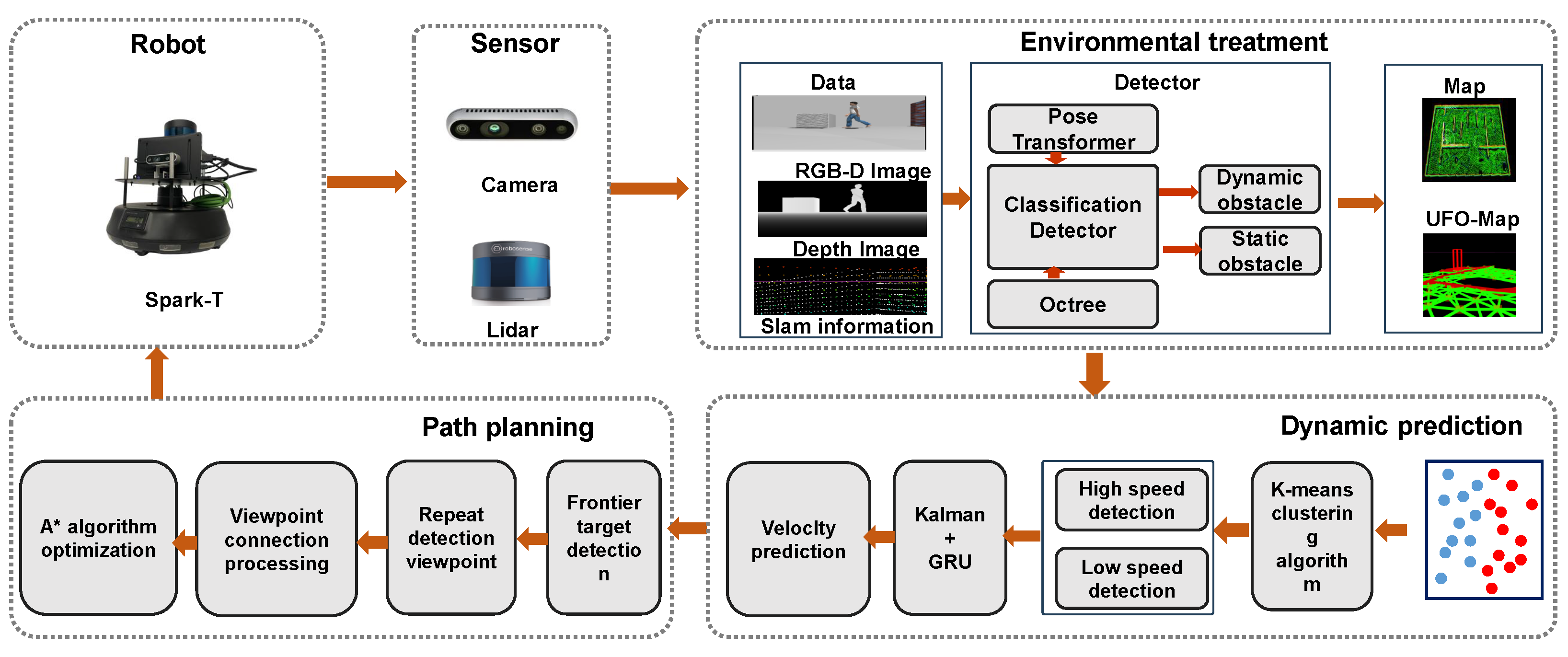
Motion planning in unknown environments with dynamic obstacles presents significant challenges. Frontier-based methods [11,12,13] and sampling-based approaches [12,13,14] are effective for incremental exploration of unknown spaces, achieving completeness or near-optimality through boundary identification, random sampling, hierarchical planning, and viewpoint integration. However, these techniques primarily focus on exploration and static mapping; their effectiveness diminishes significantly when confronted with unpredictable dynamic obstacles.

The existing motion planning approaches for dealing with dynamic obstacles include prediction-based motion planning methods, artificial potential field, and model-based methods [15,16,17,18]. The work in [15] uses avoidance actions based on the position and velocity of the robot and the obstacles. The work in [16] further refined the potential field of obstacles in the APE framework to improve the performance of online obstacle avoidance. The work in [17] uses the MPC method to represent uncertainty using the chance constraint. The work in [18] added gradient optimization and further improved the dynamic model to achieve efficient dynamic obstacle avoidance.

Effective prediction and tracking of dynamic obstacles remain challenging. To address this, we propose the “K-GRU Kalman” framework. This hybrid approach strategically integrates Kalman filtering (KF) [19,20] and Gated Recurrent Unit (GRU) networks [21,22], motivated by their complementary strengths in handling uncertainty and complex dynamics. Critically, raw sensor data undergoes initial processing via K-means clustering [23,24] for efficient obstacle segmentation (e.g., velocity-based classification [25]). The Kalman filter (KF) provides uncertainty-aware filtering and short-term state propagation, leveraging its recursive structure for real-time efficiency. The gated recurrent unit (GRU) then processes the KF estimates as refined inputs, enabling explicit recognition of motion patterns and capturing complex, nonlinear velocity variations that challenge purely stochastic models. Thus, the information flow progresses from segmentation and stochastic filtering (KF) to learned pattern modeling (GRU). This synergistic integration mitigates the limitations of each component: KF’s linearity assumptions are compensated by GRU’s ability to learn complex trajectories, while GRU’s reliance on large datasets is alleviated through KF’s robust preprocessing. By jointly leveraging uncertainty quantification through the Kalman filter (KF) and adaptive learning via gated recurrent units (GRU), the framework aims to enhance robustness in environments with mixed static and variable-speed dynamic obstacles under uncertainty.

3. Methodology

Motion planning in environments with both static and dynamic obstacles remains challenging, especially when the robot enters a completely unknown environment denoted as $M_{\mathrm{unknown}}\subset M$. The environment is incrementally discovered through frontier detection, and corresponding environmental information is acquired via viewpoints. In the presence of dynamic obstacles, the environment evolves continuously over time. Without an accurate estimation of $M_{\mathrm{known}}$, reliable viewpoints cannot be obtained, increasing the risk of collisions due to incorrect perception. Therefore, accurately determining the next position $P_i$ is crucial for safe and effective exploration. The overall framework is illustrated in Figure 1.

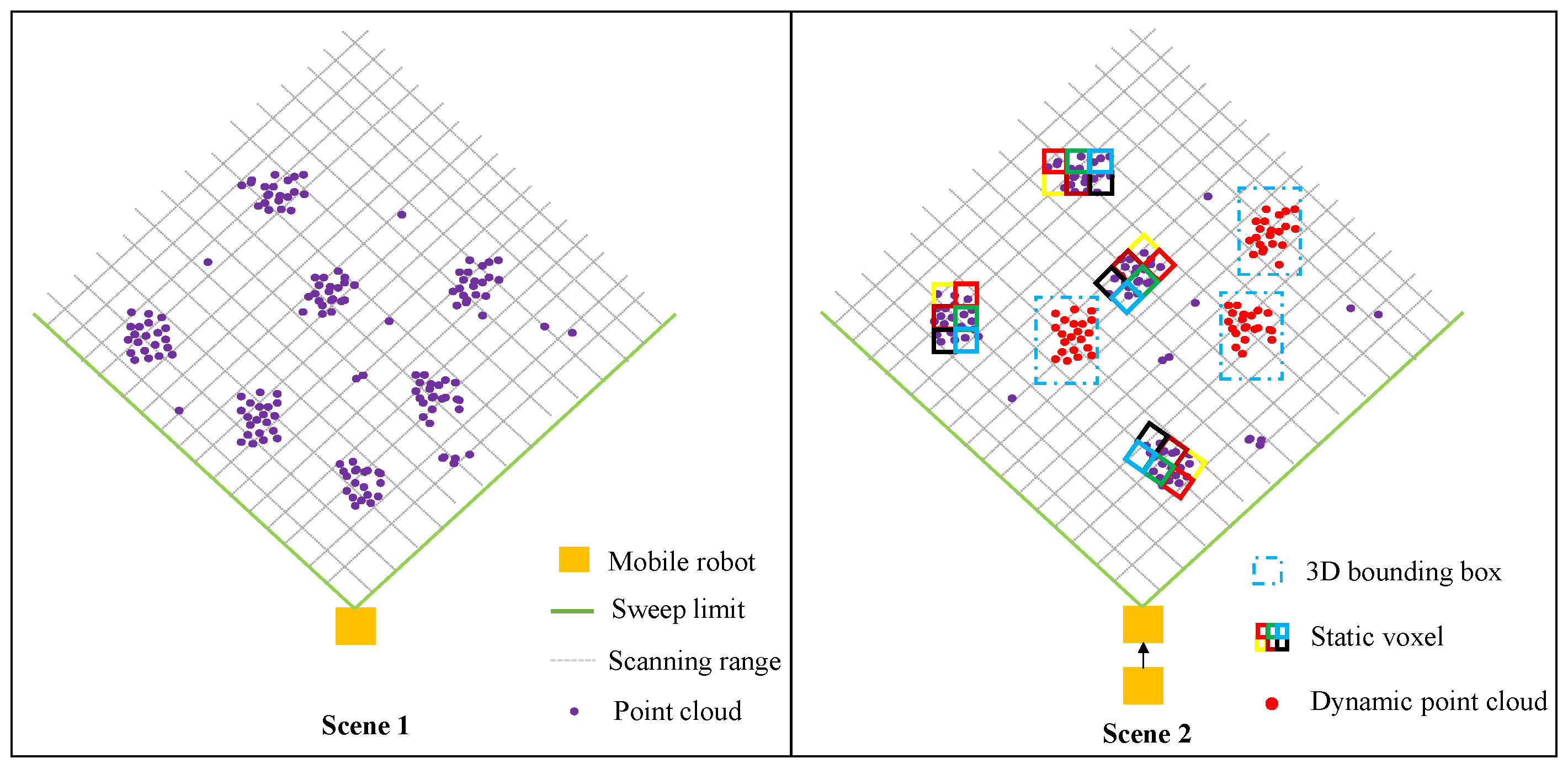
3.1. Environment Map Construction

Obstacles are categorized as either static or dynamic, with distinct representation methods adopted for each type. Figure 2 illustrates the classification of point clouds corresponding to static and dynamic obstacles.

(1) Classification of dynamic and static obstacles: In this paper, a depth camera is employed to obtain the corresponding point cloud data to classify dynamic and static obstacles. First, the 3D information is obtained. When the camera obtains point cloud data, the obstacles are represented as point cloud clusters. The corresponding point cloud cluster data is then clustered into point cloud clustering, and the corresponding center point is obtained from the point cloud clustering.

After receiving the corresponding obstacle information, the camera continuously obtains environmental images. At this point, the offset of the corresponding clustered point cloud is obtained while obtaining the corresponding image of each frame. As the static obstacle itself does not move, the offset will remain stable within the threshold. However, because of its own motion, the offset of the dynamic obstacle will be larger than the corresponding threshold if it moves.

(2) Static Obstacles: When dealing with static obstacles, LiDAR is used to obtain environmental information about static obstacles. The LiDAR on the mobile robot scans for SLAM information corresponding to the environment. After obtaining the corresponding SLAM information, the data is processed, and voxels are used to represent the corresponding environmental information. Finally, the corresponding environment information is stored in the information octree to represent the corresponding environments in three states: occupied, idle, and unknown. After the corresponding environment information is stored in the node, the corresponding environment information is processed to accelerate the traversal of the octree. When the information changes with the environment, the corresponding information begins to be automatically generated and automatically deleted, thus obtaining the maximum number of static obstacles.

3.2. Prediction of Obstacles

The proposed K-GRU Kalman method integrates three components: K-means clustering of obstacle velocity data, Kalman filtering for trajectory prediction, and a Gated Recurrent Unit (GRU) neural network for real-time tracking of dynamic obstacles. The process begins by clustering detected obstacles into low- and high-speed groups using K-means based on real-time average speed calculations. This clustering determines subsequent processing priorities: high-speed obstacles are buffered for delayed handling, while low-speed obstacles are prioritized. The Kalman filter then processes these low-speed obstacles, using historical state data (position and velocity) alongside motion models and current observations to execute prediction and correction steps. A four-dimensional state vector is constructed to represent the most recent state of each obstacle. These state vectors are serialized into temporal sequences and fed into the GRU network, which utilizes its gating mechanisms to capture long-term dependencies in obstacle motion. The GRU then directly outputs the predicted position and velocity for each low-speed obstacle at the next time step.

(1) K-means clustering: The K-means clustering algorithm is applied to the velocity data of obstacles to distinguish between low-speed and high-speed groups. The process begins by computing the average velocity of all detected obstacles. For each object i, with positions moving from $(x_i,t_i,y_i,t_i)$ to $(x_{i,t+\Delta t},y_{i,t+\Delta t})$, the average velocity is computed as follows:

$$\begin{array}{cc}\hfill v_x& ={\displaystyle \frac{x_{i,t+\Delta t}-x_{i,t}}{\Delta t}}\hfill \end{array}$$

(1)

$$\begin{array}{cc}\hfill v_y& ={\displaystyle \frac{y_{i,t+\Delta t}-y_{i,t}}{\Delta t}}\hfill \end{array}$$

(2)

Subsequently, the centroids are initialized by randomly selecting $k=2$ initial points, denoted as $c_1^{\left(0\right)}$ and $c_2^{\left(0\right)}$, from the velocity data. Next, at each iteration t, clusters are assigned based on the nearest principle. Each sample $v_i=(v_x,v_y)$ is assigned the same label as the nearest centroid. If $\left|\right|v_i-c_1^{(t-1)}{\left|\right|}^2<\left|\right|v_i-c_2^{(t-1)}{\left|\right|}^2$, then it is classified as belonging to the low-speed group; otherwise, if $\left|\right|v_i-c_1^{(t-1)}{\left|\right|}^2>\left|\right|v_i-c_2^{(t-1)}{\left|\right|}^2$, it is classified as belonging to the high-speed group.

After separating into low-speed and high-speed groups, centroids are updated. For each class j, the new centroid $c_j^{\left(t\right)}$ is the mean of all samples $v_i=(v_x,v_y)$ assigned to that class, given as follows:

$$c_j^{\left(t\right)}={\displaystyle \frac{1}{|S_j|}}\sum _{i\in S_j}{v}_i$$

(3)

where $S_j$ is a set containing all sample indices assigned label j at time $t-1$. The iterative process will continue until convergence is reached, which is manifested by the fact that the centroid no longer changes significantly or that the maximum number of preset iterations is reached.

(2) Kalman Filter: Based on the classification of low-speed and high-speed groups using the K-means clustering algorithm, the high-speed group is stored and the trajectory prediction is performed on the large number of low-speed groups. Here, the update equations of the Kalman filter for predicting the system’s state at the next time step are employed. The state prediction and update are computed as shown in Equations (4) and (5), respectively:

$$x_{t+1|t}=A{x}_{t|t-1}+w_t$$

(4)

$$x_{t+1}=x_{t+1|t}+K(y-Hx)$$

(5)

where A is the state transition matrix, $w_t$ is the process noise, K is the Kalman gain, x, y are observations, and H is the observation matrix. In this experiment, a Brownian motion model [26] is adopted, where state transitions are sampled from a probability distribution, typically a normal distribution. In this scenario, the system matrix A is set to the identity matrix $I_n$, where $n=4$, which represents position and velocity. The velocity of positions $(x,y)$ is observed; thus, these elements are included in the state vector. In a two-dimensional space, the state of each obstacle can be represented as $\mathbf{x}={[x,y,v_x,v_y]}^T$, where $v_x$ and $v_y$ are the velocities in the x and y directions, respectively.

Utilizing the random walk model as the underlying motion model and assuming no control input, the system matrix A is defined as follows:

$$A=\left[\begin{array}{cccc}1& 0& \Delta t& 0\\ 0& 1& 0& \Delta t\\ 0& 0& 1& 0\\ 0& 0& 0& 1\end{array}\right]$$

(6)

Here, $\Delta t$ denotes the time step. The new position includes a random perturbation added to the previous position, modeled by the process noise covariance $Q_t$. The state transition is given by $x_{t+1}=A{x}_{t-1}+w_t$, where $w_t\sim \mathcal{N}(0,Q_t)$ represents zero-mean Gaussian process noise.

Since all four state variables are directly observable, the observation matrix H is defined as a $4\times 4$ identity matrix. Accordingly, at each time step $t+1$, the Kalman filter generates a prediction based on the previous estimate $x_{j,t}$.

$$x_{j,t+1}=A{x}_{j,t}+B\mu +w_t$$

(7)

Here, the parameter $\mu$ represents the control input, and B is the control input coefficient.

Subsequently, the predicted value is corrected based on actual observations:

$$x_{j,t+1}=x_{j,t+1}y+K(y-Hx)$$

(8)

where K is the Kalman gain, P represents error covariance, and R represents observation noise covariance.

(3) GRU Neural Network: Following the aforementioned steps, a sequence predicted by the Kalman filter is obtained, providing position and velocity information of obstacles at each time step. These data are organized into a four-dimensional vector ${\mathbf{x}}_t=[x_{pos},y_{pos},v_x,v_y]$, which is then fed into the GRU network.

Firstly, the hidden state $h_0$ is initialized, serving as the memory unit that stores past information within the model. Then, for each frame, the following operations are performed:

The update gate and reset gate are computed as shown in Equations (9) and (10), respectively:

$$z_t=\sigma (W_z[h_{t-1},x_t]+b_z)$$

(9)

$$r_t=\sigma (W_r[h_{t-1},x_t]+b_r)$$

(10)

The candidate hidden state is generated by combining the current input with the adjusted previous hidden state through the reset gate:

$${\tilde{h}}_t=tanh\left(W_h[r_t\odot h_{t-1},x_t]+b_h\right)$$

(11)

The final hidden state at time step t is then computed by interpolating between the previous hidden state and the candidate state, weighted by the update gate:

$$h_t=(1-z_t)\odot h_{t-1}+z_t\odot {\tilde{h}}_t$$

(12)

After processing all time steps, the final hidden state $h_T$—which encodes information from the entire input sequence—is obtained. This vector serves as a high-level abstract representation of the overall dynamic trajectory features. Typically, $h_T$ is passed through one or more fully connected layers to generate the final prediction. For predicting the position and velocity of obstacles at the next time step, the following formula is employed:

$${\widehat{x}}_{t+1}=W_0{h}_t+b_0$$

(13)

where ${\widehat{x}}_{t+1}$ represents the model’s estimate of the future state, and $W_0$ and $b_0$ are parameters of the output layer.

The GRU network is composed of two layers: (1) GRU Layer: This is a variant of a recurrent neural network (RNN) comprising 50 hidden units, accepting input with a shape of (1, 4), i.e., processing one sequence at a time, with each sequence having four features. Unlike standard RNNs, GRU employs update and reset gates to control information flow. (2) Dense Fully Connected Layer: This layer concatenates all outputs generated by the preceding layer and is used to generate the final prediction results. The model is configured with four output nodes corresponding to the predicted positions $x,y$ and their velocities ${\displaystyle \frac{dx}{dt}},{\displaystyle \frac{dy}{dt}}$.

After obtaining enhanced predictions for the low-speed group, the high-speed group’s data undergoes similar prediction processing. The predictions for the high-speed group are then updated after those of the low-speed group to provide real-time updates for subsequent obstacle avoidance, thus reducing the computational load of parallel computing.

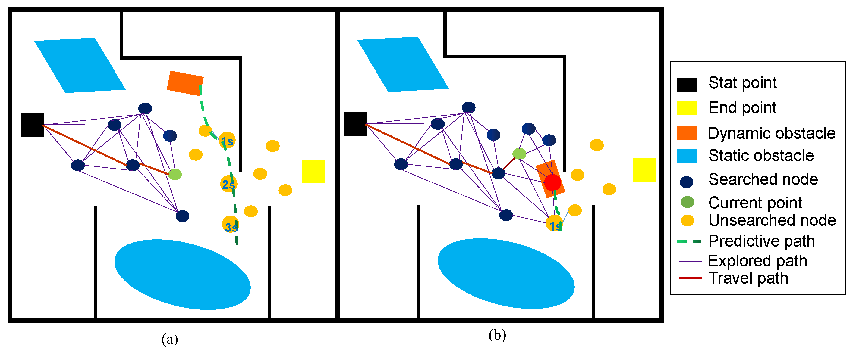
3.3. Motion Planning

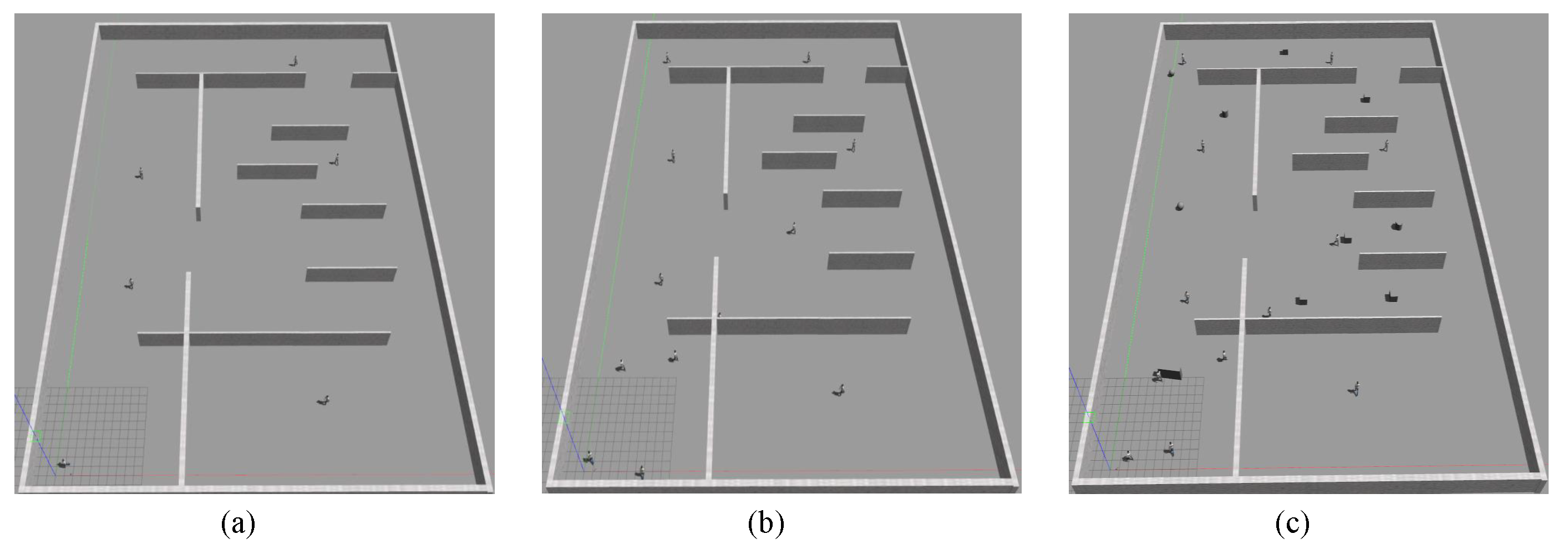
Prediction of dynamic obstacles is integrated with a sampling-based method to achieve path planning.

(1) Sample point generation: The multi-sensor fusion method acquires environmental information within the complex space M for analysis. As the robot moves, the sensing range of the sensor at step i is denoted by $f_i$. With continuous motion, the perception regions at consecutive steps overlap, represented by $f_i\cap f_{i+1}$. According to the corresponding boundary information obtained, the occupied map $M_{\mathrm{oc}}$, the free map $M_{\mathrm{fr}}$, and the corresponding unknown map $M_{\mathrm{unknown}}$ in the map are obtained. After obtaining the corresponding free map $M_{\mathrm{fr}}$, the corresponding observation viewpoint I is randomly generated in the free area, and in the corresponding observation viewpoint I, the environmental information around the viewpoint is obtained.

(2) Node queries and connections Given that this environment state needs to be continuously updated, new nodes do not directly establish a connection after they are generated. We use a judgment method similar to a time window to query the judgment points. As the motion of the obstacle is predicted, the potential for interference between the viewpoint and the obstacles can be calculated at a subsequent moment. If we predict that there will be an obstacle in the field at a viewpoint in the next moment, the viewpoint will not be added to our path map. As shown in Figure 3, we calculate the time it takes for each moving obstacle to approach the viewpoint, at which point in time it is not taken into account in planning. To better realize the planning of the robot, the planning time of the robot is considered to be:

$$T_p=T_1\cap T_2\cap T_3\cap T_v$$

(14)

where $T_p$ is used to limit the robot’s driving when the robot’s planning time is at the intersection of three times. $T_1$, $T_2$, and $T_3$ represent the time interval for the dynamic obstacle to reach viewpoint 1, viewpoint 2, and viewpoint 3, respectively, and $T_v$ is the time for the robot to move to these three positions. The effective time is obtained by calculating the intersection of the robot’s arrival time and the obstacle’s arrival time $T_p$. If the corresponding viewpoint selection is not completed within the intersection time, the selection will be made again within the time. Although the planning speed will be slower than other planning algorithms, dynamic obstacles can be avoided within the maximum fault tolerance.

(3) Path optimization: When the mobile robot is driving, collisions with obstacles can be avoided to a great extent by selecting the viewpoint ahead. But, this will lead to a situation where the solution is not the optimal path. At this time, in order to better compensate for the path problem, the corresponding path optimization is adopted, in which the position of the next coordinate $P_{i+1}$ performs the corresponding calculations:

$$P_{i+1}=P_i+T_p\times v$$

(15)

where v represents the current speed of the robot, and the corresponding speed is calculated as:

$$v=\sum _{k=1}^n{\displaystyle \frac{C_k}{n}}{v}_0$$

(16)

where n is all obstacles within the implementation, $v_0$ represents the initial speed of the robot, and $C_k$ is the corresponding predictor. The predictors are calculated as follows:

$$C_k=ln{\displaystyle \frac{V_i}{{\delta }_k}}\eta$$

(17)

where $\eta$ is the normalization factor, and $V_i$ is the predicted speed information of the obstacle.

${\delta }_k$ denotes the Euclidean distance between the mobile robot and the predicted position, corresponding to coordinates $(x_s,y_s)$ used to estimate the position of dynamic obstacle t.

$${\delta }_k=\sqrt{{(x_s-x_i)}^2+{(y_s-y_i)}^2}$$

(18)

4. Experiments

Experimental validation of the proposed algorithm was conducted in both simulated and physical environments. The simulation platform was powered by an Intel Core i9-13700K CPU and an NVIDIA RTX 4000 GPU. To evaluate the performance of the proposed algorithm, it is deployed in a simulation environment and verified using the Jackal robot platform. For real-world deployment, a Spark robot, featuring an Intel Core i7-8700K CPU and 32 GB of RAM, was used as the experimental platform.

4.1. Ablation Experiment

(1) Parameter settings: The LiDAR sensing range of the mobile robot in the simulation environment is 6 m, the frequency is 10 Hz, the depth camera sensing range is 3 m, the viewing angle is 87°, and the maximum speed of the robot is 1.5 m/s. In Figure 4a–c, the starting point of the navigation movement is set at 1 m above the lower right corner of the wall, while the end point is set at 1 m above the upper left corner of the wall.

(2) Implementation: The environment shown in Figure 4 contains a limited number of dynamic and static obstacles. The dynamic obstacles move back and forth within the environment at velocities ranging from 0.4 m/s to 0.6 m/s.

(3) Algorithm Configurations

• Algorithm 1: This algorithm is derived from the TARE algorithm proposed in [13].
• Algorithm 2: This configuration excludes the prediction algorithm module from the system. The path optimization algorithm is incorporated on top of Algorithm 1 to improve performance.
• Ours: This refers to the algorithm proposed in this paper.

As shown in

Table 1. Performance of ablation experiments in different environments.

Environment	Algorithm	Time(s)			Success Rate (%)
		min	avg	max
	Algorithm 1	172.3	186.7	222.5	90
Scenario (a)	Algorithm 2	169.4	180.2	204.3	70
	Ours	166.7	184.3	210.2	90
	Algorithm 1	197.4	208.8	230.2	60
Scenario (b)	Algorithm 2	186.4	210.4	226.9	40
	Ours	192.6	202.3	220.4	80
	Algorithm 1	203.1	226.7	233.2	40
Scenario (c)	Algorithm 2	207.2	233.8	235.6	20
	Ours	208.4	221.3	238.9	60

, all methods perform well in low-complexity dynamic scenes. However, with a substantial increase in obstacle density, both the obstacle avoidance success rate and target accessibility of Algorithm 1 and Algorithm 2 decline noticeably, especially in Scene C. This limitation primarily stems from their inability to effectively coordinate avoidance among dynamic obstacles moving at varying speeds, resulting in a higher collision risk. Additionally, in densely cluttered environments, factors such as occlusions in the robot’s perception system and limited sensing range further increase the likelihood of collisions in complex scenarios like Scene C. In contrast, the method proposed herein significantly enhances motion robustness by integrating a dynamic trajectory prediction model and optimizing the node selection strategy. Although this improvement may cause a slight decrease in overall system efficiency, it substantially increases navigation reliability under challenging conditions.

4.2. Experiments on Prediction

In the simulated environments, three sets of comparative experiments were designed within a 10 m × 10 m area: five low-speed moving obstacles and one high-speed obstacle; nine low-speed obstacles and one high-speed obstacle; nine low-speed obstacles and one ultra-high-speed obstacle. During data acquisition, low-speed obstacles were simplified as circular mobile robots with a radius of 0.15 m and speed threshold below 0.2 m/s. In contrast, high-speed obstacles were simplified similarly with a radius of 0.15 m and speed threshold above 1.1 m/s. In the third comparative experiment, the speed threshold of the ultra-high-speed obstacle was above 3 m/s. We obtained position and velocity information in the X and Y directions of obstacle Brownian motion for 10 s in the simulated 10 m × 10 m environment of the three comparative experiments, forming our dataset.

To quantitatively evaluate the performance of our system, we compared the proposed method with traditional and state-of-the-art dynamic obstacle trajectory predictors on mobile robot platforms [27,28].

Table 2. Comparison of different algorithms on ADE and FDE metrics across various scenes.

Environment	Algorithm	ADE	FDE
Scene1	ours	0.024	0.053
	LSTM [29]	0.067	0.292
	Kalman [19]	1.250	2.033
	Particle filter [30]	1.250	2.033
	UKF  [31]	2.281	4.360
Scene2	ours	0.021	0.020
	LSTM [29]	0.096	0.108
	Kalman [19]	1.182	2.375
	Particle filter [30]	1.166	2.375
	UKF [31]	2.150	5.466
Scene3	ours	0.026	0.058
	LSTM [29]	0.110	0.298
	Kalman [19]	1.278	2.033
	Particle filter [30]	1.277	2.033
	UKF [31]	2.208	5.784

presents the comparison of Average Displacement Error (ADE) [28] and Final Displacement Error (FDE) [28] for both position and velocity estimates. As shown in Table 2, the proposed method achieves superior accuracy in positional estimation. Experimental results indicate that the inferior performance of other methods stems from their inability to differentiate between low-speed and high-speed obstacles, causing positional jumps in fast-moving obstacles that introduce noise and reduce trajectory estimation accuracy for slow-moving objects.

The results also show that, compared to Method II, our trajectory prediction system delivers improved velocity predictions while maintaining comparable positional accuracy. Although Method II employs Recurrent Neural Networks (RNNs) and Long Short-Term Memory (LSTM) networks for trajectory prediction, it struggles to produce accurate results when there are significant variations in displacement magnitudes.

In contrast, our proposed method uses a speed-based classification approach that stores only limited data on high-velocity dynamic obstacles. By focusing first on accurately predicting a large number of slower-moving objects, the method reduces noise introduced by faster entities, thereby yielding more precise trajectory estimates.

4.3. Experiments in the Real World

A D435 depth camera was used, featuring an RGB frame rate of 30 fps, a minimum depth range of 28 cm, and a field of view (FOV) of 87° × 58°. To thoroughly evaluate system performance, additional dynamic obstacles with varied sizes and speeds were introduced in the real test environment, with more complex obstacle placements. For safety considerations, the maximum speed of dynamic obstacles was limited to 0.4 m/s.

As demonstrated in Figure 5, experimental results and analyses conducted in real-world scenarios confirm that the proposed system enables accurate perception and identification of both static and dynamic obstacles in complex, dynamic environments. The system robustly detects 3D bounding boxes of dynamic obstacles and predicts their motion states, including velocity variations. Leveraging this environmental awareness and predictive capability, the robot effectively navigates toward its designated target. Furthermore, comprehensive field tests in diverse, unstructured environments validate the robustness and generalization of the proposed perception and planning framework. These results demonstrate successful perception, recognition, and motion planning performance in complex scenes containing both static and dynamic elements.

5. Conclusions and Future Work

A comprehensive framework for dynamic obstacle avoidance and trajectory prediction is proposed, applicable to both simulated and real-world environments. The method begins by dynamically classifying obstacles, followed by accurate prediction of high- and low-speed motion patterns of dynamic obstacles. Overall motion planning efficiency is enhanced through optimization of node connectivity strategies. Experimental results from both simulation and real-world scenarios demonstrate that the proposed framework significantly improves motion safety in dynamic environments. Future work will focus on addressing motion planning challenges under perception-constrained conditions such as occlusion. Moreover, further improvements in motion safety and trajectory planning robustness are anticipated through optimization of multimodal perception fusion and dynamic risk assessment mechanisms.

References

1. Roth-Tabak, Y.; Jain, R. Building an environment model using depth information. Computer 1989, 22, 85–90. [Google Scholar] [CrossRef]
2. Hornung, A.; Wurm, K.M.; Bennewitz, M.; Stachniss, C.; Burgard, W. OctoMap: An efficient probabilistic 3D mapping framework based on octrees. Auton. Robot. 2013, 34, 189–206. [Google Scholar] [CrossRef]
3. Duberg, D.; Jensfelt, P. UFOMap: An Efficient Probabilistic 3D Mapping Framework That Embraces the Unknown. IEEE Robot. Autom. Lett. 2020, 5, 6411–6418. [Google Scholar] [CrossRef]
4. Cai, Y.; Kong, F.; Ren, Y.; Zhu, F.; Lin, J.; Zhang, F. Occupancy Grid Mapping Without Ray-Casting for High-Resolution LiDAR Sensors. IEEE Trans. Robot. 2024, 40, 172–192. [Google Scholar] [CrossRef]
5. Lin, J.; Zhu, H.; Alonso-Mora, J. Robust Vision-based Obstacle Avoidance for Micro Aerial Vehicles in Dynamic Environments. In Proceedings of the IEEE International Conference on Robotics and Automation (ICRA), Paris, France, 31 May–4 June 2020. [Google Scholar]
6. He, B.; Li, H.; Wu, S.; Wang, D.; Zhang, Z.; Dong, Q. FAST-Dynamic-Vision: Detection and Tracking Dynamic Objects with Event and Depth Sensing. In Proceedings of the IEEE/RSJ International Conference on Intelligent Robots and Systems (IROS), Prague, Czech Republic, 25–29 October 2021; pp. 3071–3078. [Google Scholar] [CrossRef]
7. He, J.; Sun, Z.; Cao, N.; Ming, D.; Cai, C. Target Attribute Perception Based UAV Real-Time Task Planning in Dynamic Environments. In Proceedings of the IEEE/RSJ International Conference on Intelligent Robots and Systems (IROS), Detroit, MI, USA, 1–5 October 2023; pp. 888–895. [Google Scholar] [CrossRef]
8. Newcombe, R.A.; Izadi, S.; Hilliges, O.; Molyneaux, D.; Kim, D.; Davison, A.J. KinectFusion: Real-time dense surface mapping and tracking. In Proceedings of the 10th IEEE International Symposium on Mixed and Augmented Reality, Basel, Switzerland, 26–29 October 2011; pp. 127–136. [Google Scholar] [CrossRef]
9. Eppenberger, T.; Cesari, G.; Dymczyk, M.; Siegwart, R.; Dubé, R. Leveraging Stereo-Camera Data for Real-Time Dynamic Obstacle Detection and Tracking. In Proceedings of the IEEE/RSJ International Conference on Intelligent Robots and Systems (IROS), Las Vegas, NV, USA, 12–16 October 2020; pp. 10528–10535. [Google Scholar] [CrossRef]
10. Chen, G.; Dong, W.; Peng, P.; Alonso-Mora, J.; Zhu, X. Continuous Occupancy Mapping in Dynamic Environments Using Particles. IEEE Trans. Robot. 2023, 40, 64–84. [Google Scholar] [CrossRef]
11. Yamauchi, B. A frontier-based approach for autonomous exploration. In Proceedings of the 1997 IEEE International Symposium on Computational Intelligence in Robotics and Automation CIRA ’97. “Towards New Computational Principles for Robotics and Automation”, Monterey, CA, USA, 28 July–1 August 1997; pp. 146–151. [Google Scholar] [CrossRef]
12. Zhu, B.; Zhang, Y.; Chen, X.; Shen, S. FUEL: Fast UAV Exploration Using Incremental Frontier Structure and Hierarchical Planning. IEEE Robot. Autom. Lett. 2021, 6, 779–786. [Google Scholar] [CrossRef]
13. Cao, C.; Zhu, H.; Choset, H.; Zhang, J. TARE: A hierarchical framework for efficiently exploring complex 3D environments. Front. Robot. AI Syst. 2021, 5. [Google Scholar] [CrossRef]
14. LaValle, S. Rapidly-Exploring Random Trees: A New Tool for Path Planning; Research Report 9811; Department of Computer Science, Iowa State University: Ames, IA, USA, 1998. [Google Scholar]
15. Fiorini, P.; Shiller, Z. Motion, planning in dynamic environments using velocity obstacles. Int. J. Robot. Res. 1998, 17, 760–772. [Google Scholar] [CrossRef]
16. Malone, N.; Chiang, H.T.; Lesser, K.; Oishi, M.; Tapia, L. Hybrid dynamic moving obstacle avoidance using a stochastic reachable-set-based potential field. IEEE Trans. Robot. 2017, 33, 1121–1138. [Google Scholar] [CrossRef]
17. Blackmore, I.; Ono, M.; Williams, B.C. Chance-Constrained Optimal Path Planning With Obstacles. IEEE Trans. Robot. 2011, 27, 1080–1094. [Google Scholar] [CrossRef]
18. Wang, T.; Ji, J.; Wang, Q.; Xu, C.; Gao, F. Autonomous Flights in Dynamic Environments with Onboard Vision. In Proceedings of the IEEE/RSJ International Conference on Intelligent Robots and Systems (IROS), Prague, Czech Republic, 25–29 October 2021; pp. 1966–1973. [Google Scholar] [CrossRef]
19. Kalman, R.E. A New Approach to Linear Filtering and Prediction Problems. J. Basic Eng. 1960, 82, 35–45. [Google Scholar] [CrossRef]
20. Welch, G.; Bishop, G. An Introduction to the Kalman Filter; University of North Carolina at Chapel Hill Chapel Hill: Chapel Hill, NC, USA, 2006. [Google Scholar]
21. Cho, K.; van Merrienboer, B.; Gulcehre, C.; Bahdanau, D.; Bougares, F.; Schwenk, H.; Bengio, Y. Learning phrase representations using RNN encoder-decoder for statistical machine translation. In Proceedings of the Conference on Empirical Methods in Natural Language Processing (EMNLP), Doha, Qatar, 25–29 October 2014. [Google Scholar]
22. Chung, J.; Gulcehre, C.; Cho, K.; Bengio, Y. Empirical evaluation of gated recurrent neural networks on sequence modeling. arXiv 2014, arXiv:1412.3555. [Google Scholar]
23. Jain, A.K. Data clustering: 50 years beyond K-means. Pattern Recognit. Lett. 2010, 31, 651–666. [Google Scholar] [CrossRef]
24. Lloyd, S. Least squares quantization in PCM. IEEE Trans. Inf. Theory 1982, 28, 129–137. [Google Scholar] [CrossRef]
25. Aryal, M. Object Detection, Classification, and Tracking for Autonomous Vehicle. Master’s Thesis, Grand Valley State University, Allendale, MI, USA, 2018. [Google Scholar]
26. Karatzas, I.; Shreve, S.E. Brownian Motion. In Brownian Motion and Stochastic Calculus; Springer: New York, NY, USA, 1998; pp. 47–127. [Google Scholar]
27. Ondruska, P.; Posner, I. Deep Tracking: Seeing Beyond Seeing Using Recurrent Neural Networks. Proc. AAAI Conf. Artif. Intell. 2016, 30, 1. [Google Scholar] [CrossRef]
28. Alahi, A.; Goel, K.; Ramanathan, V.; Robicquet, A.; Fei-Fei, L.; Savarese, S. Social LSTM: Human Trajectory Prediction in Crowded Spaces. In Proceedings of the IEEE Conference on Computer Vision and Pattern Recognition, Las Vegas, NV, USA, 26 June–1 July 2016; pp. 961–971. [Google Scholar]
29. Hochreiter, S.; Schmidhuber, J. Long Short-Term Memory. Neural Comput. 1997, 9, 1735–1780. [Google Scholar] [CrossRef]
30. Djuric, P.M. Particle Filtering. IEEE Signal Process. Mag. 2003, 20, 19–38. [Google Scholar] [CrossRef]
31. Wan, E.A.; Merwe, R.V.D. The unscented Kalman filter for nonlinear estimation. In Proceedings of the IEEE 2000 Adaptive Systems for Signal Processing, Communications, and Control Symposium (Cat. No.00EX373), Lake Louise, AB, Canada, 10–13 September 2000; pp. 153–158. [Google Scholar]
Figure 1. Motion planning framework for unknown dynamic environments: acquiring multi-sensor data (camera/LiDAR) enables dynamic–static obstacle modeling, feeding velocity prediction modules where K-means analysis generates motion forecasts, ultimately driving trajectory optimization for collision-free navigation.
Applsci 15 07551 g001
Figure 2. Classification of dynamic and static obstacle point clouds. Combinations of several solid squares indicate the static obstacles, and blue dashed rectangles indicate the bounding boxes of dynamic obstacles.
Applsci 15 07551 g002
Figure 3. (a) illustrates the generation of the robot’s viewpoint at the current position along with the predicted information of relevant obstacles, while (b) depicts the robot’s movement based on the generated viewpoint and the corresponding prediction data.
Applsci 15 07551 g003
Figure 4. Scene (a) includes six dynamic obstacles; scene (b) includes twelve dynamic obstacles; and scene (c) contains twelve dynamic obstacles along with ten static obstacles.
Applsci 15 07551 g004
Figure 5. Dynamic obstacle prediction in real-world environments using the K-GRU Kalman framework with dynamic bounding boxes. (a) perspective generation for robots in static environments, (b) single obstacle detection and (c) detection of multi-dynamic obstacles.
Applsci 15 07551 g005