A Fiber-Optic Six-Axis Force Sensor Based on a 3-UPU-Compliant Parallel Mechanism


Abstract
1. Introduction
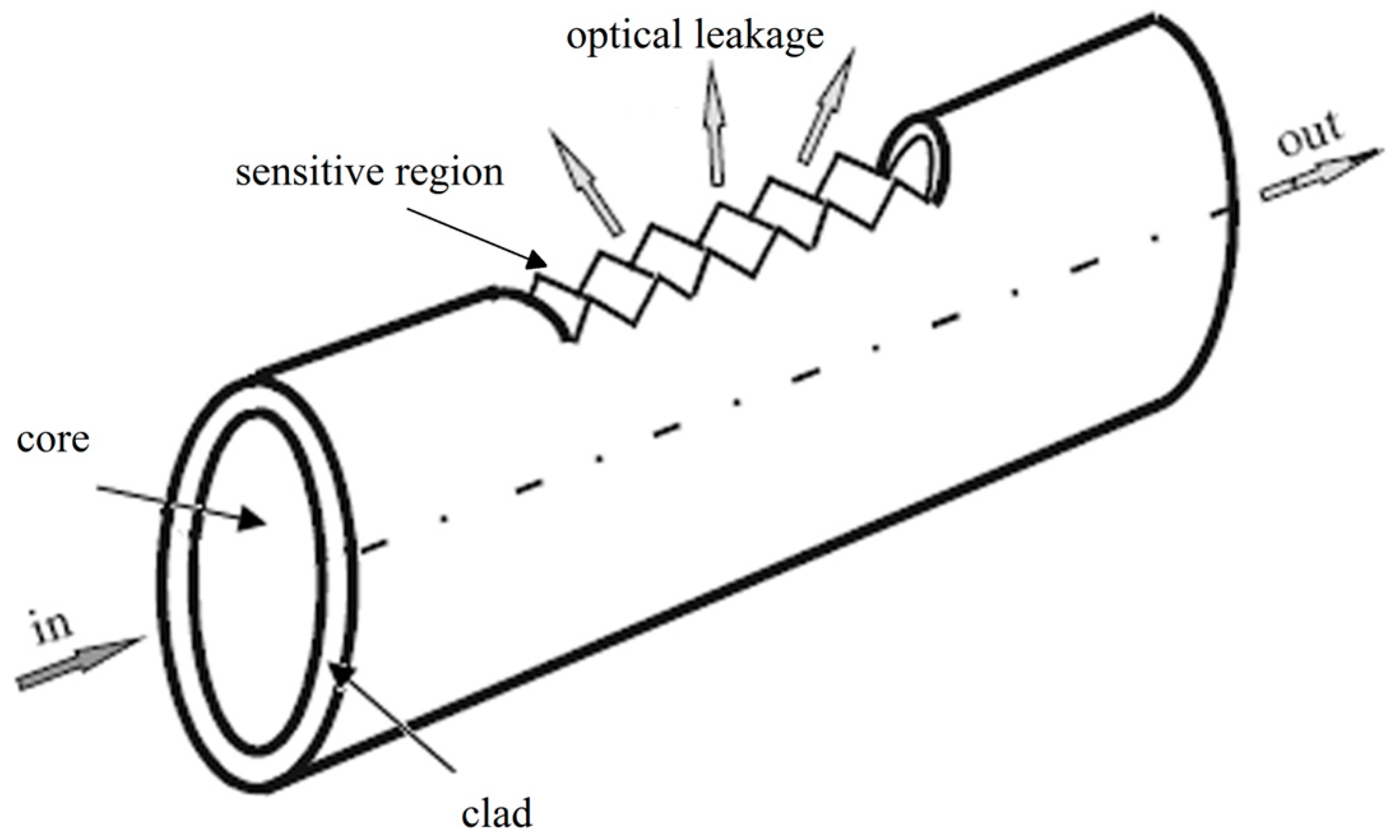
2. Bending-Sensitive Optical Fiber
2.1. Characteristics of Bending-Sensitive Optical Fiber
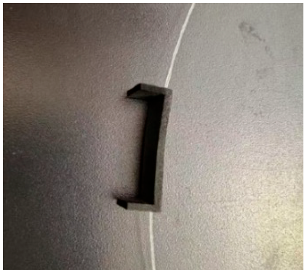
2.2. Encapsulation of Bending-Sensitive Optical Fiber
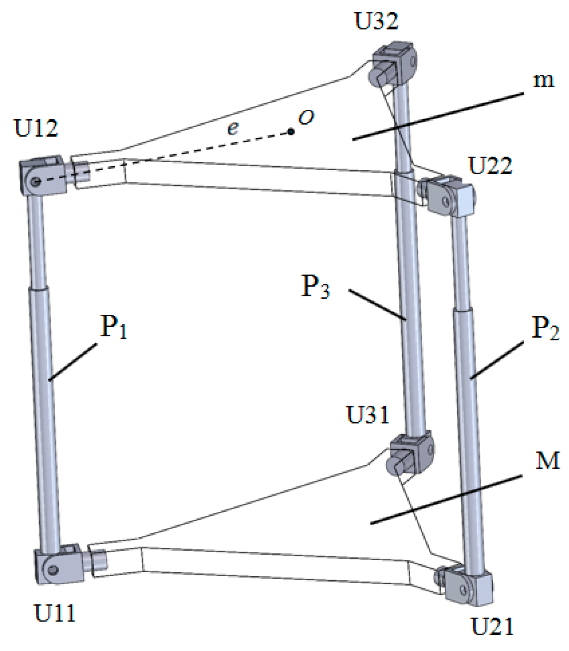
3. Structure Design and Detection Principle of Six-Axis Force Sensor
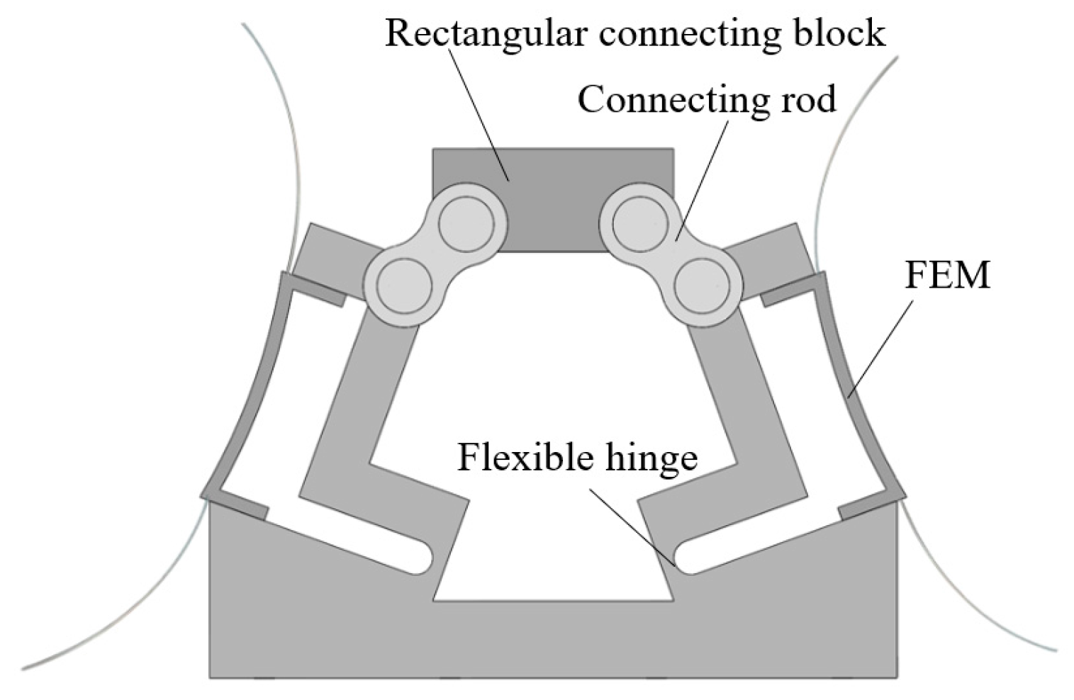
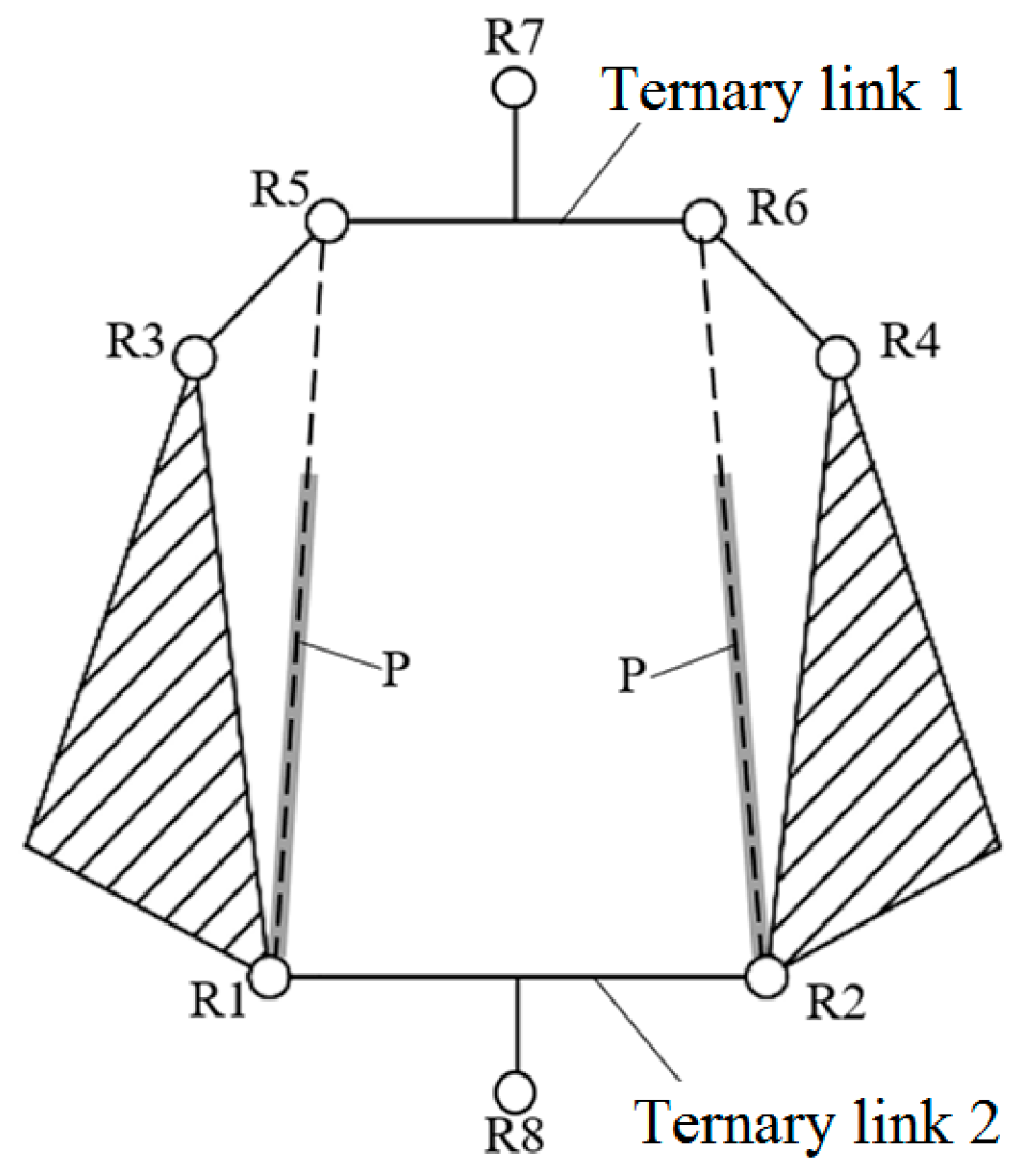
3.1. Structural Design
3.2. Force Detection Principle
4. Analysis of the Force Mapping Matrix for the Six-Axis Force Sensor
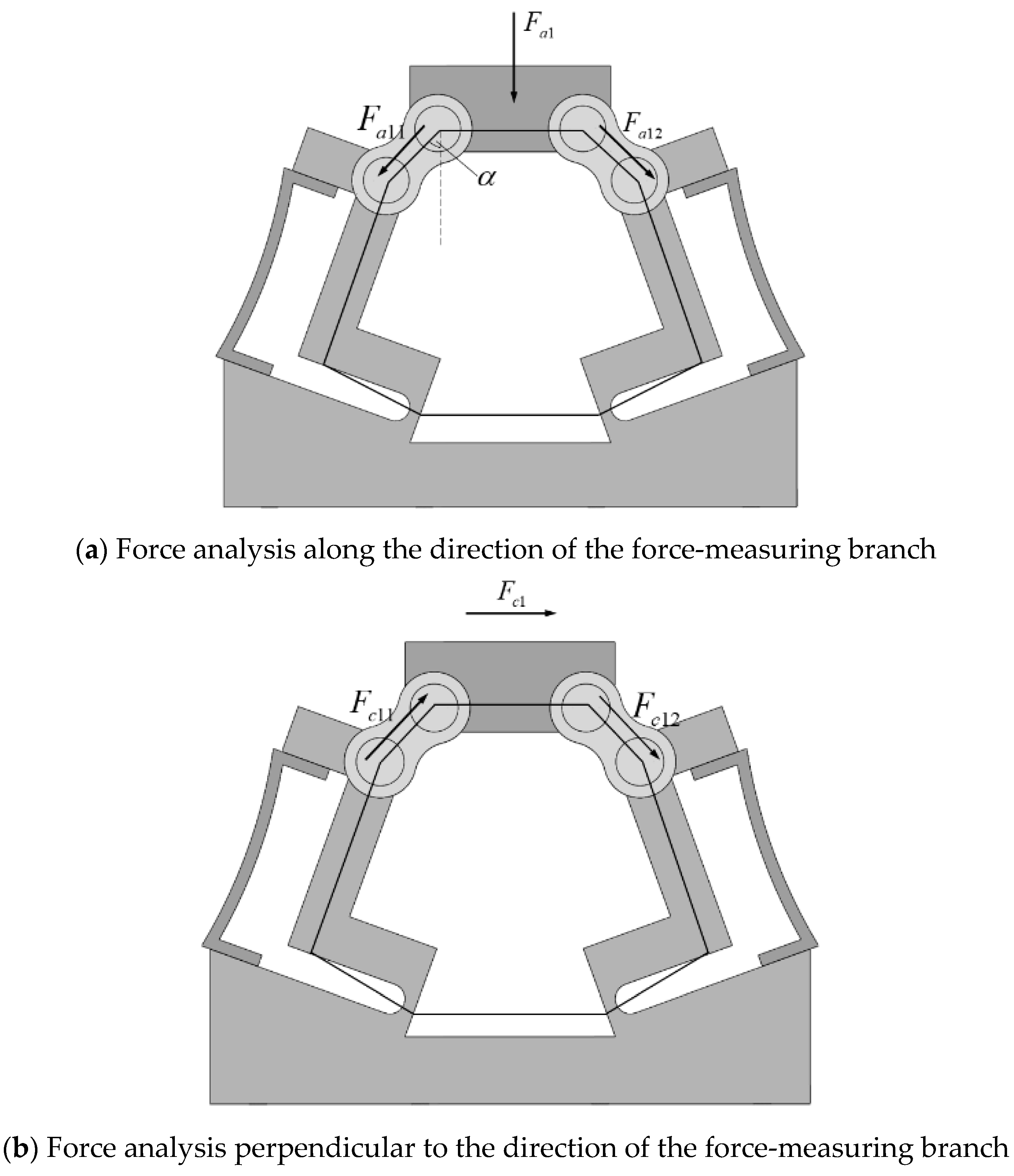
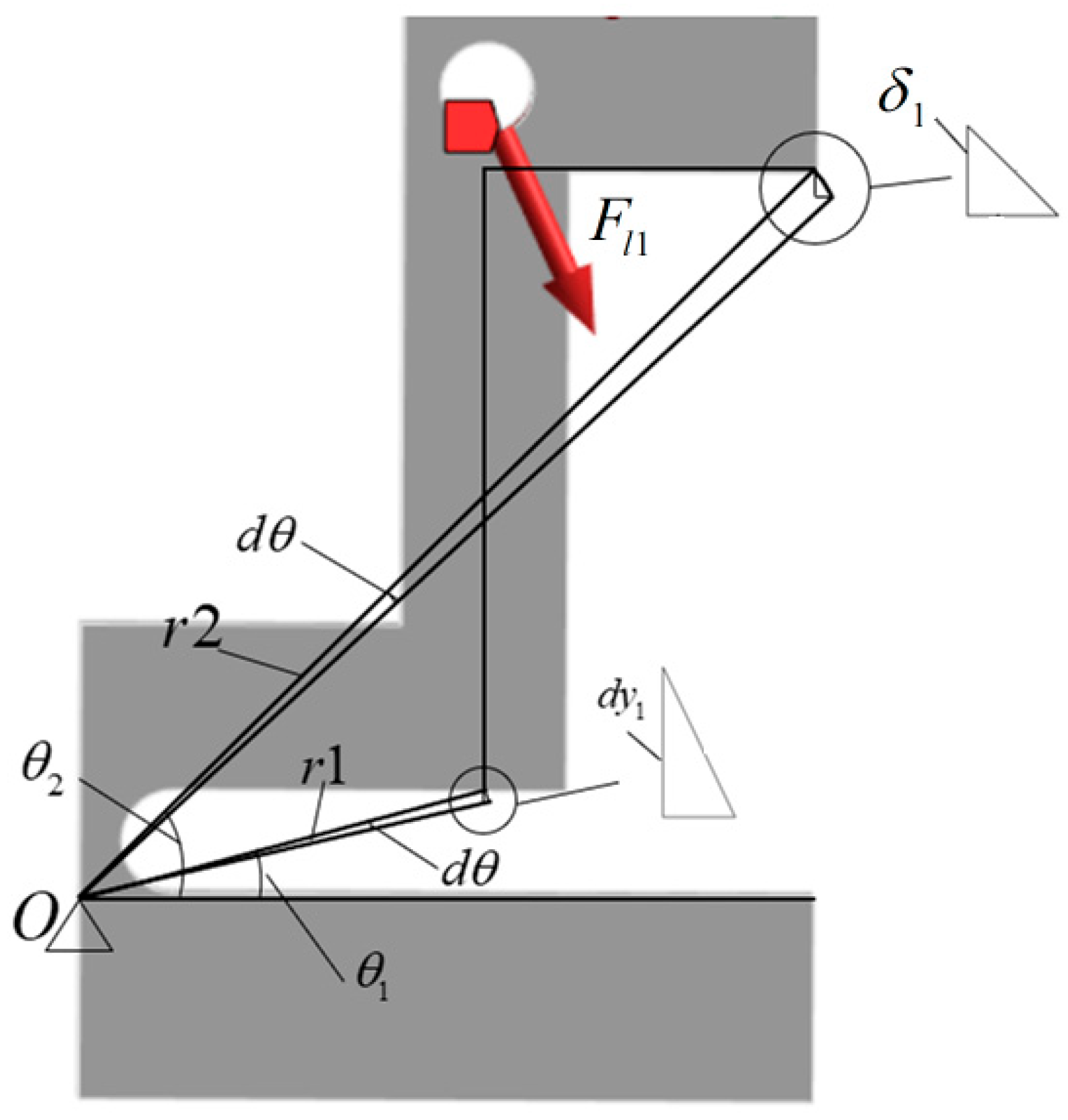
4.1. Static Analysis of the Sensor
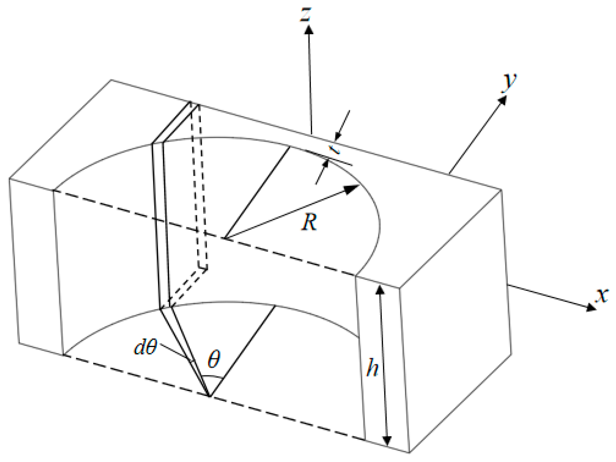
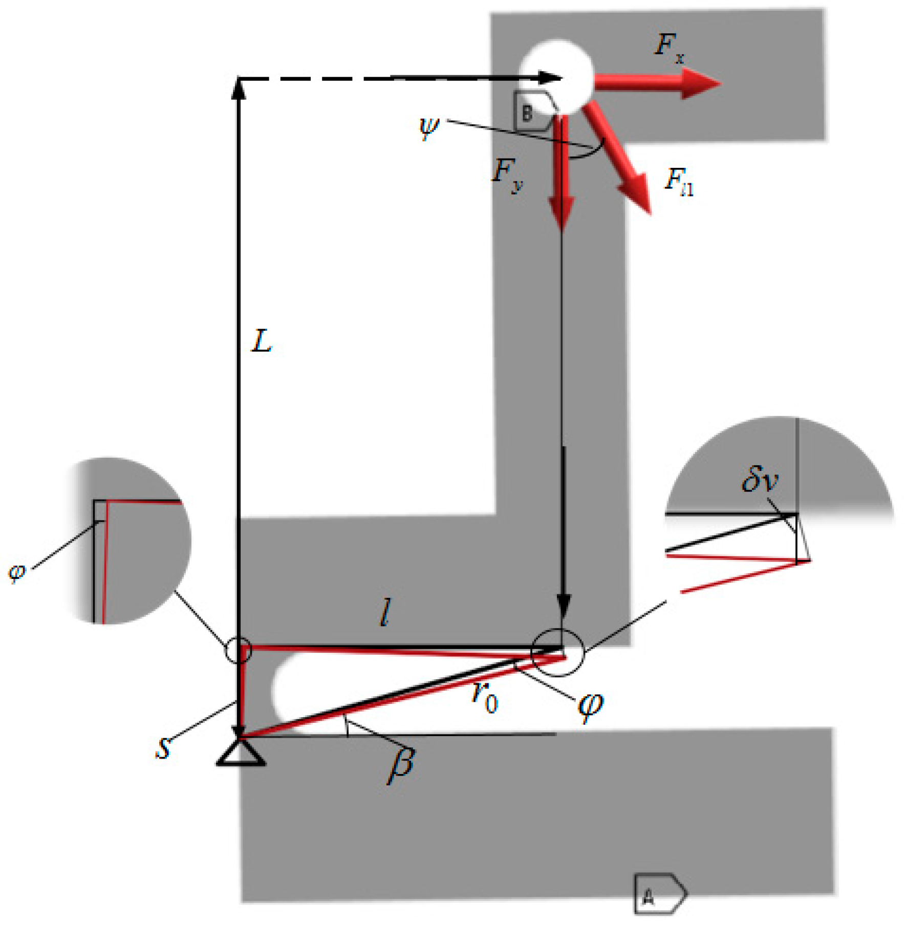
4.2. Stiffness Analysis of the Force-Measuring Branch
5. Experiments and Results Analysis
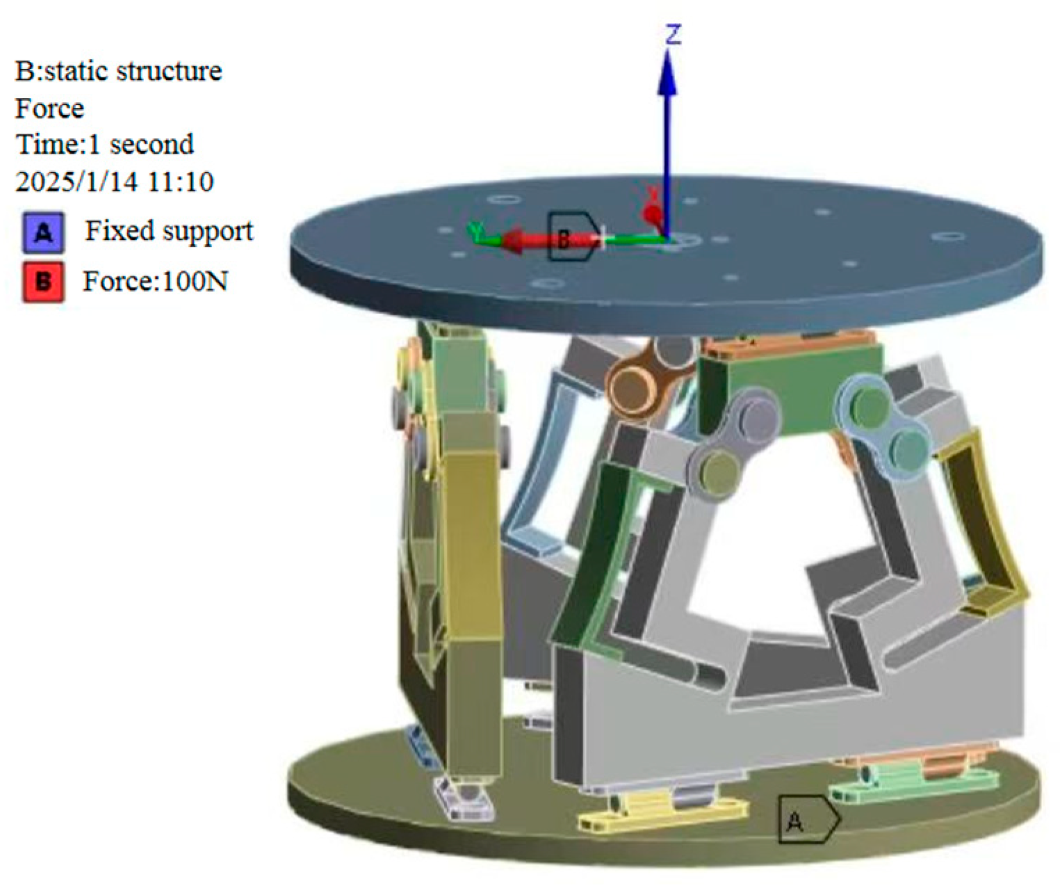
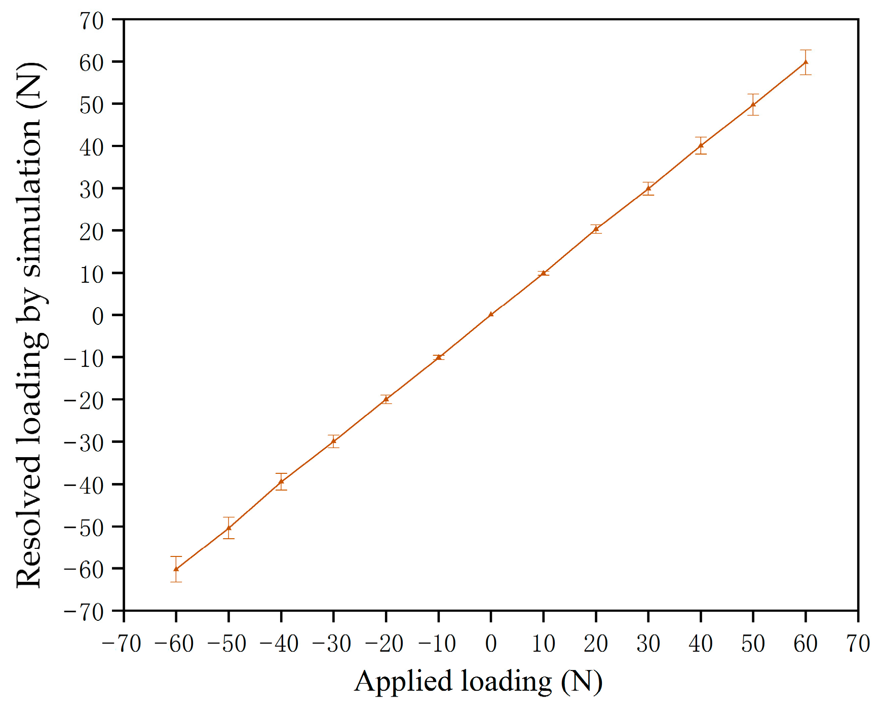
5.1. Simulation
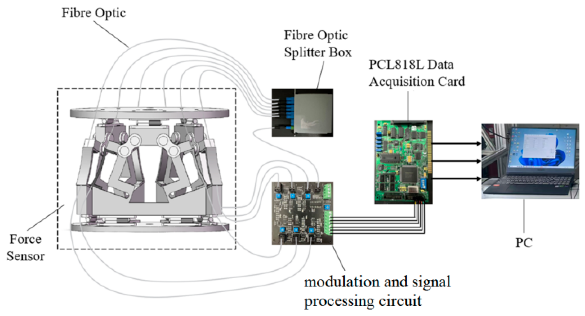
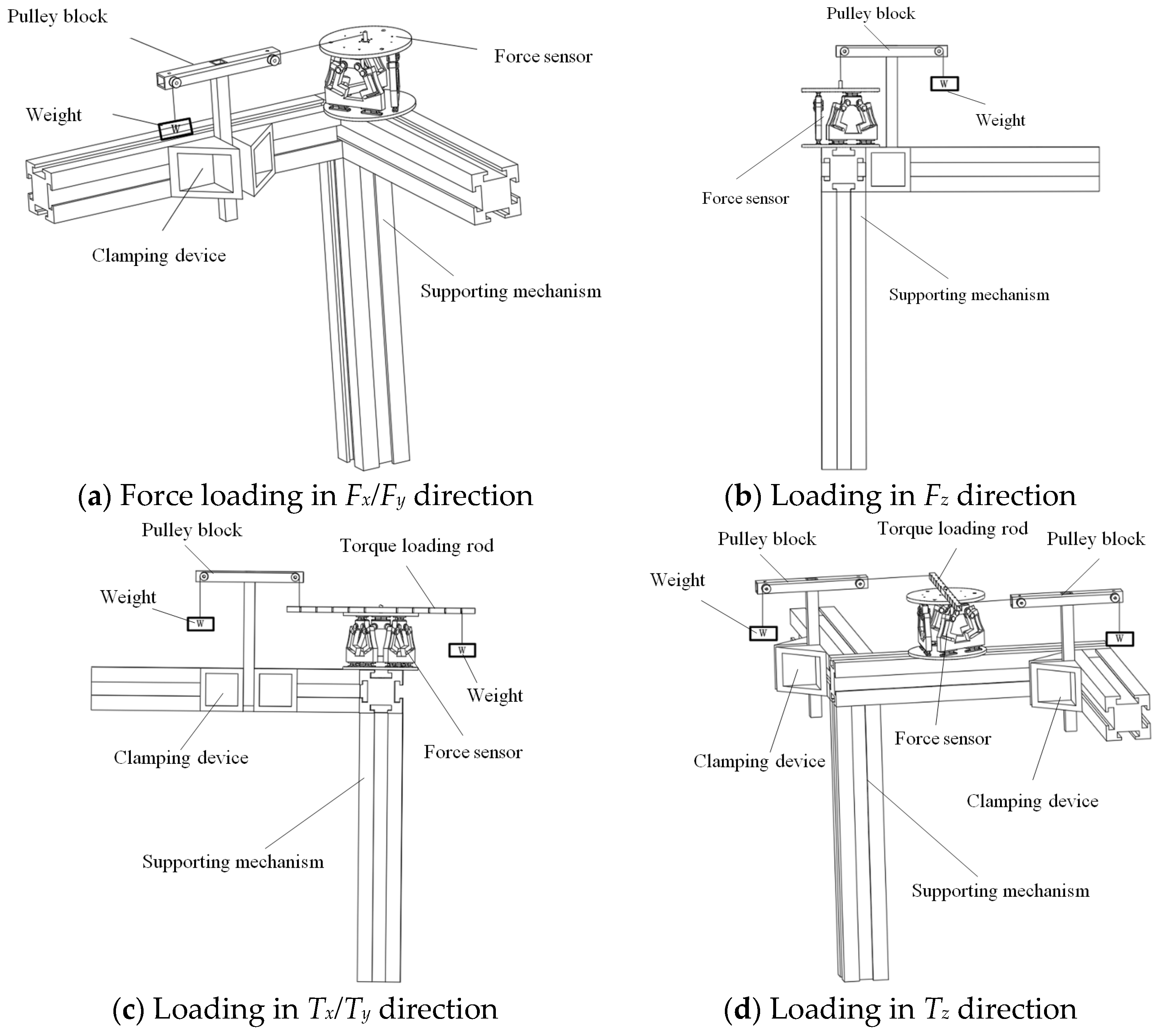
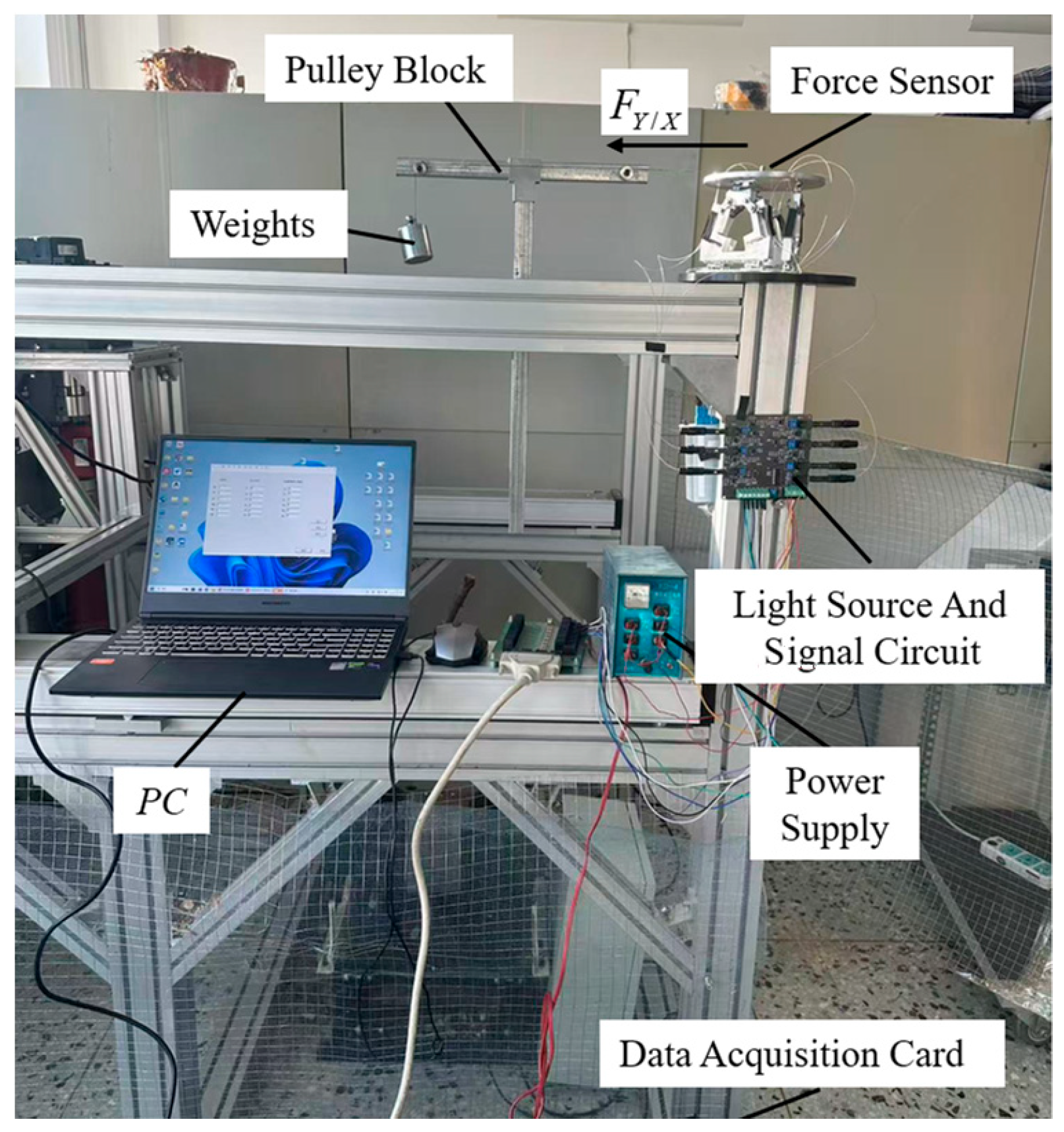
5.2. Experiment
5.3. Results and Analysis
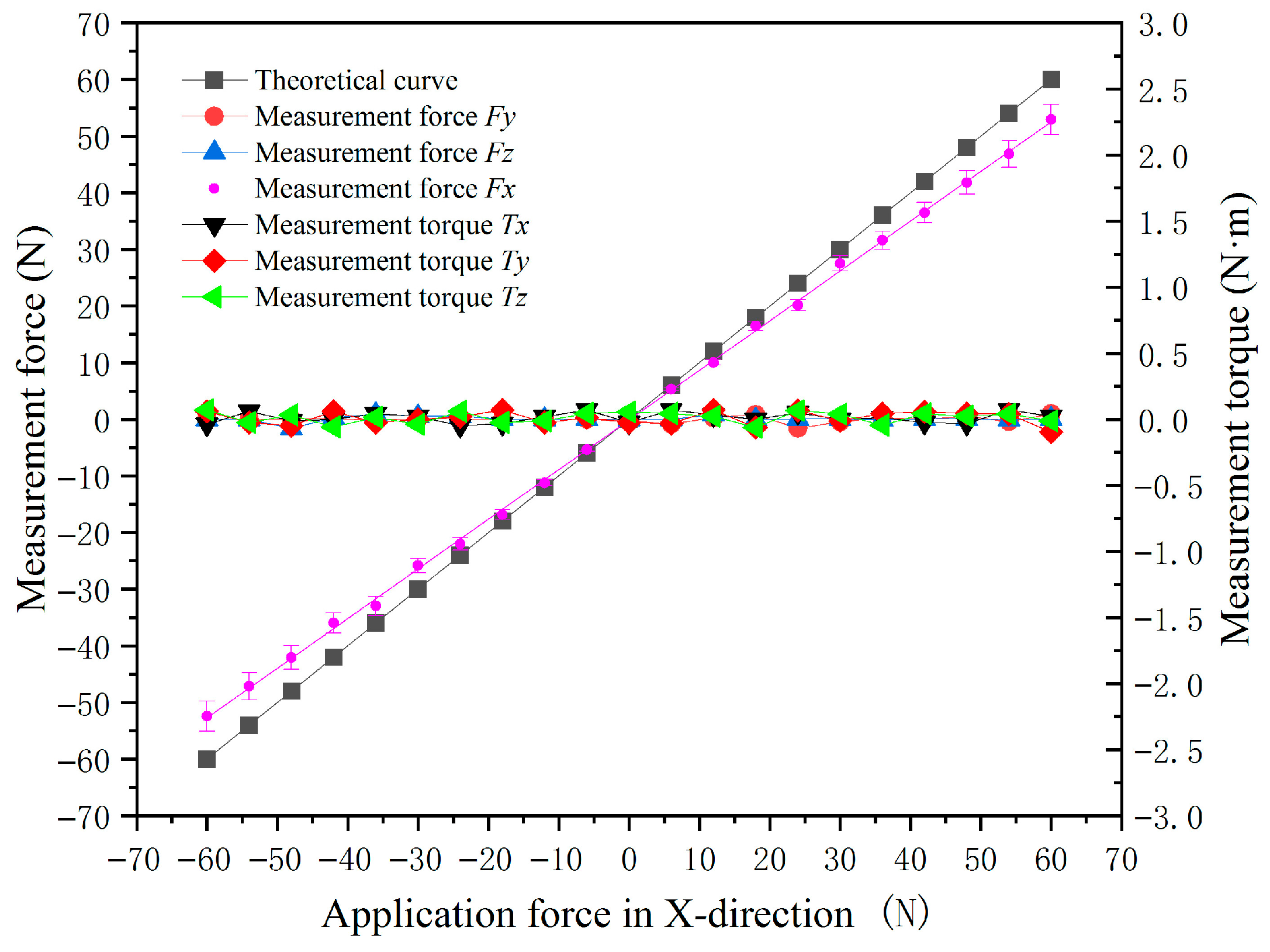
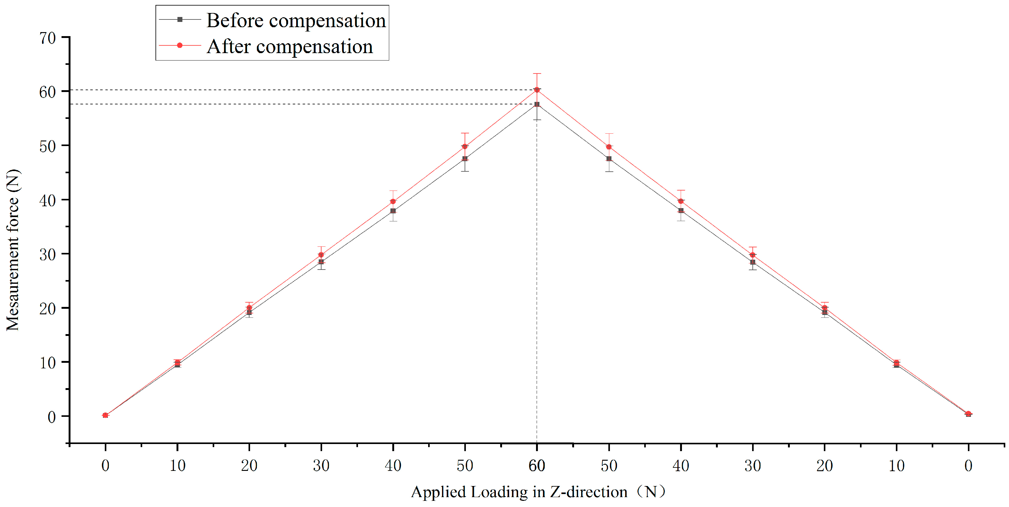
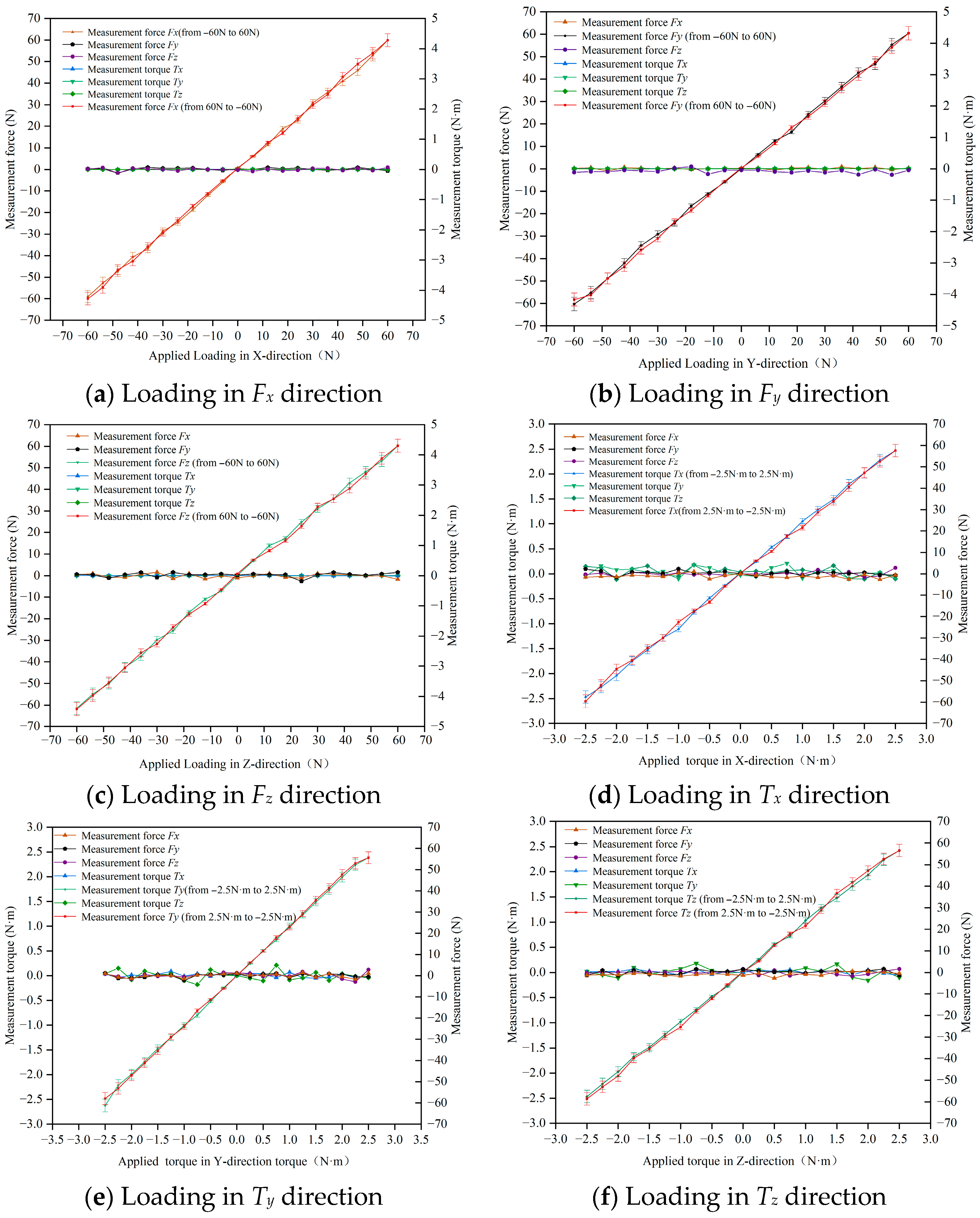
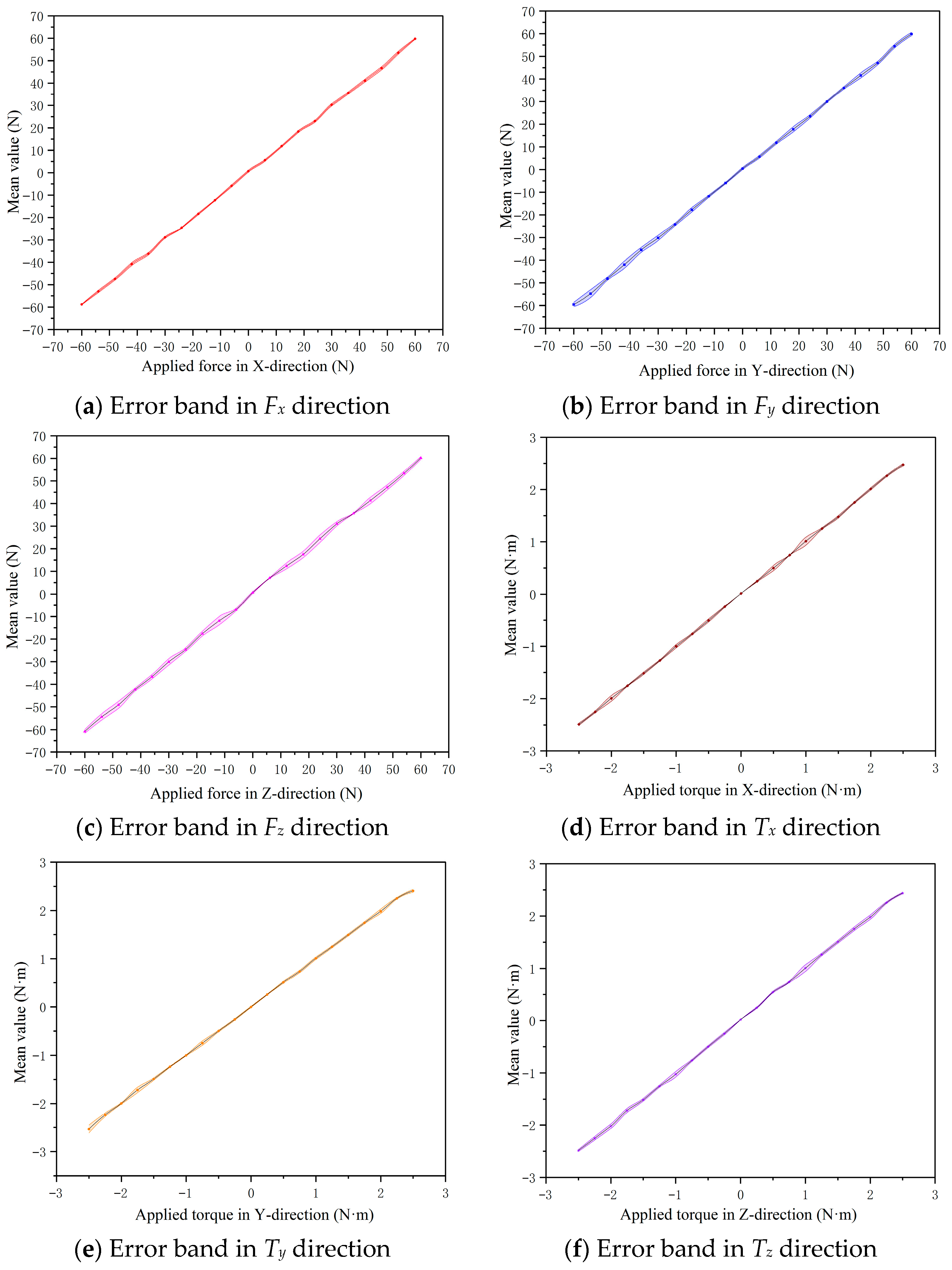
5.3.1. Accuracy and Hysteresis
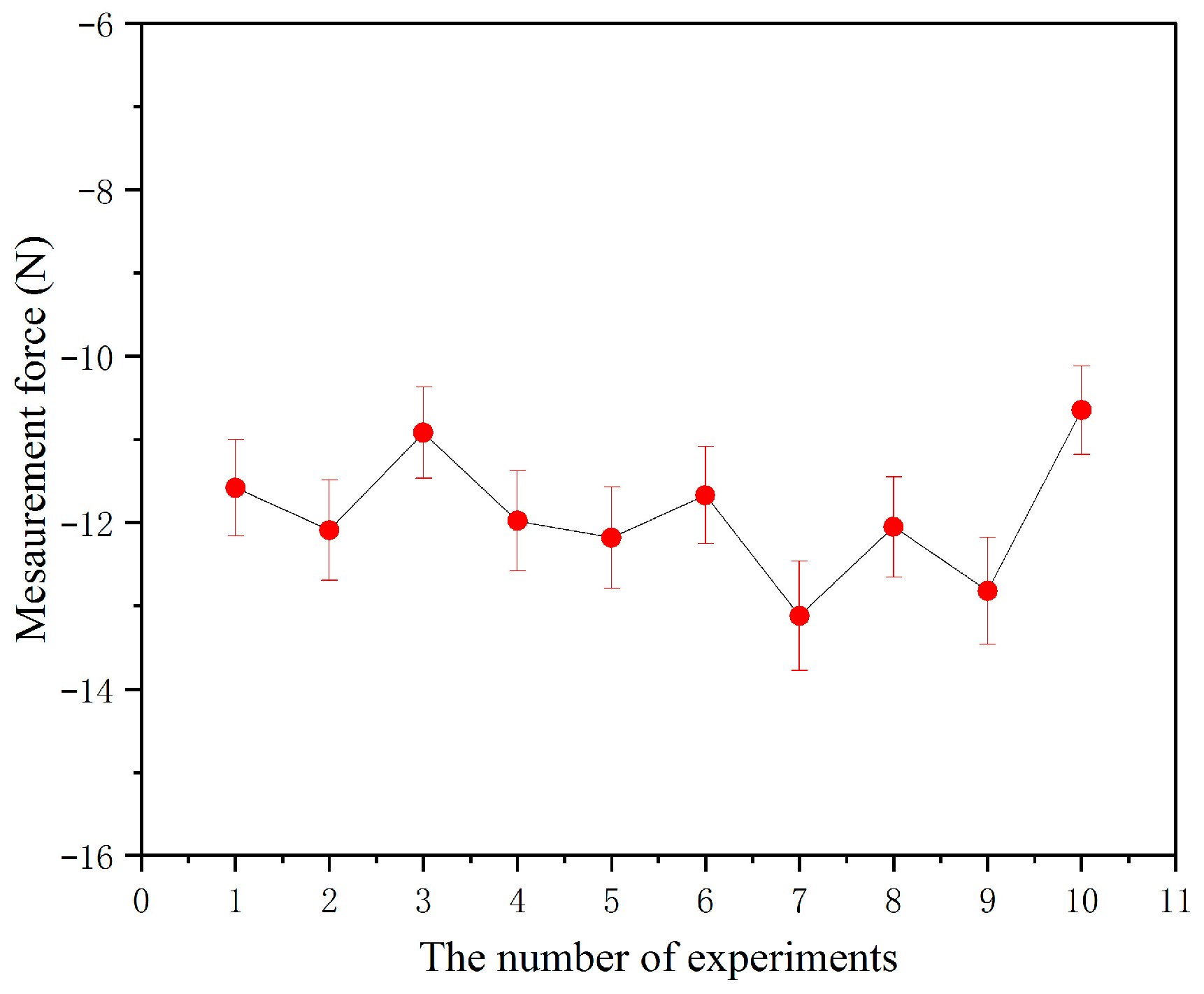
5.3.2. Repeatability
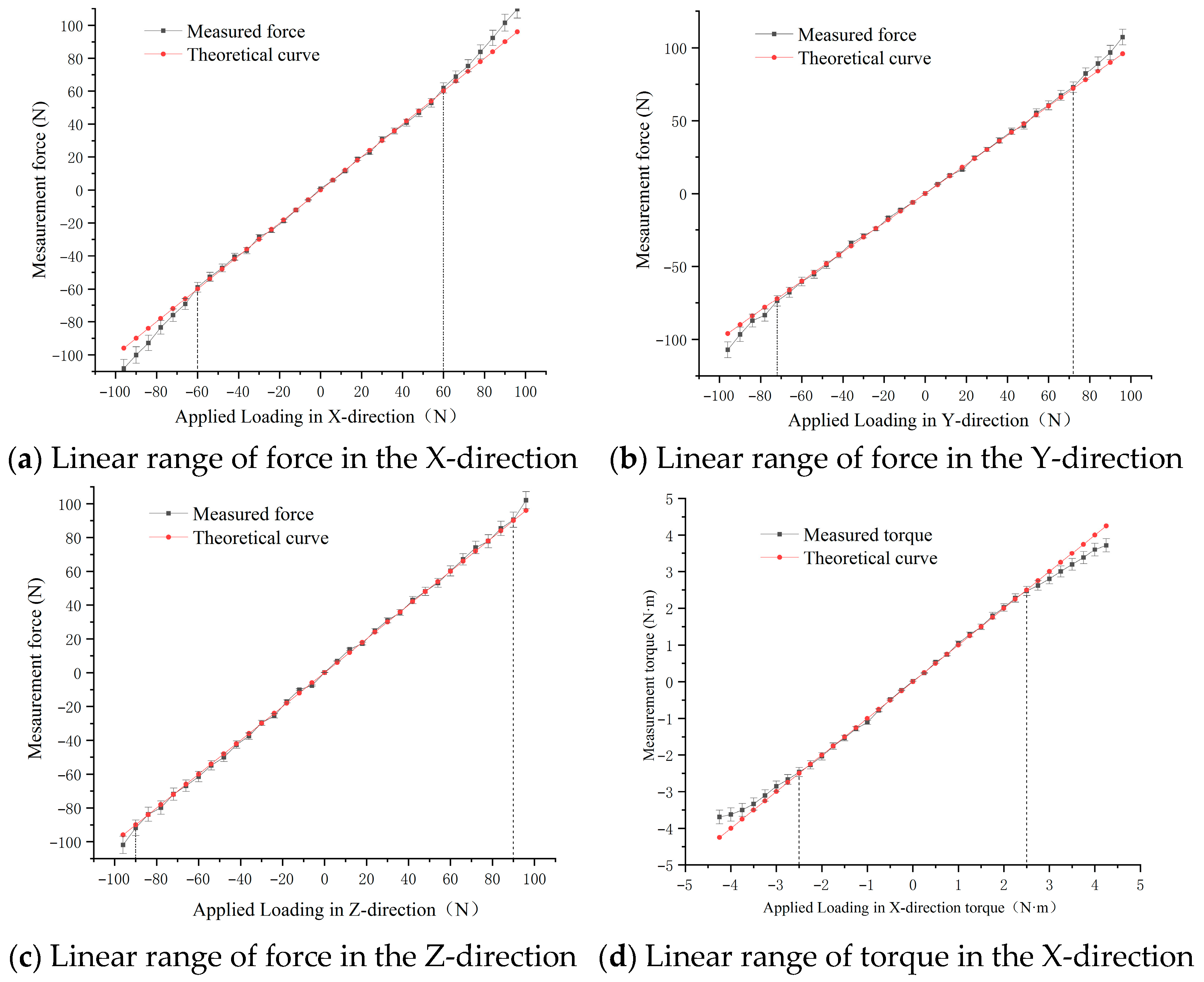
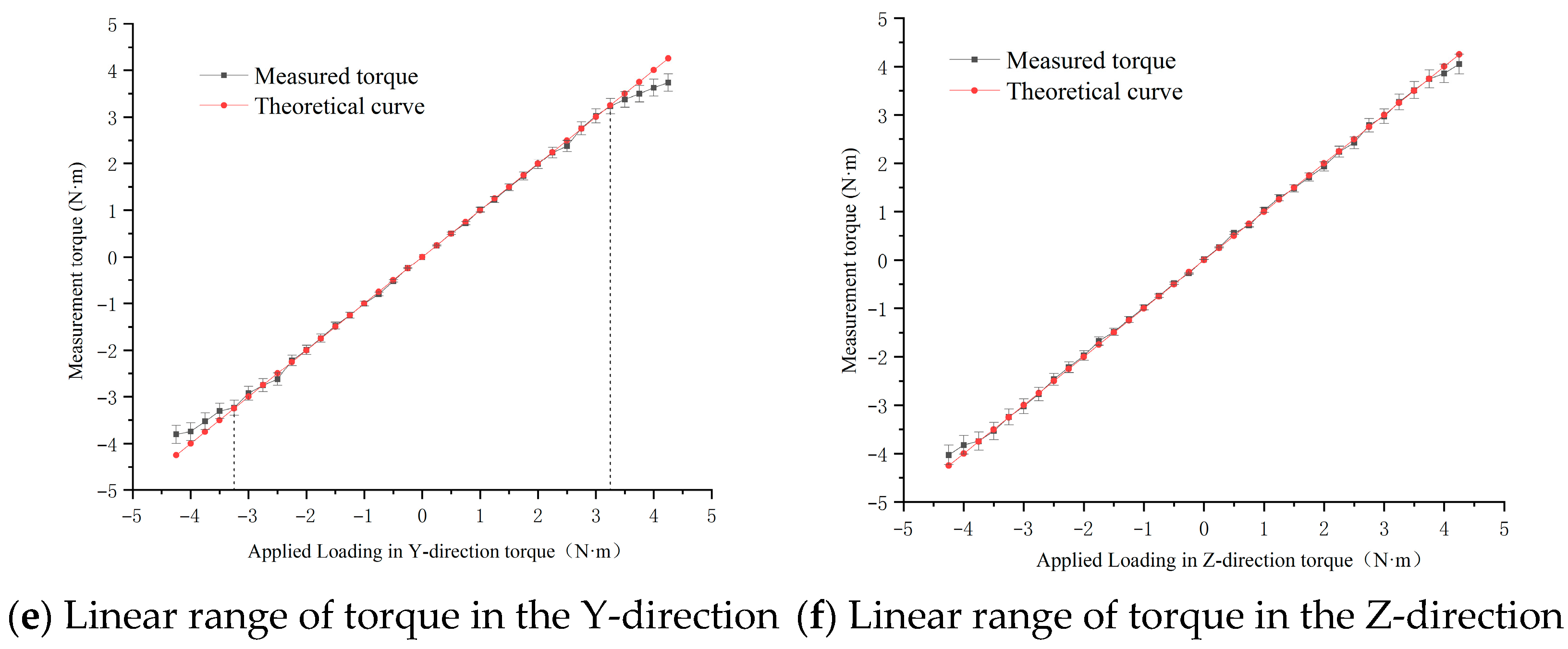
5.3.3. Linear Range and Strength Limits
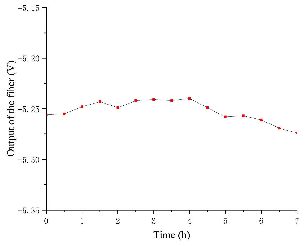
5.3.4. Thermal Effects
6. Conclusions
Author Contributions
Funding
Institutional Review Board Statement
Informed Consent Statement
Data Availability Statement
Conflicts of Interest
References
- Ogihara, T.; Kokubo, Y.; Heki, K.; Igarashi, K.; Hirano, H.; Ishii, K.; Negishi, S.; Shimizu, T.; Morikawa, K.; Hoshino, T. Development of a device for measuring bite force on individual teeth using a capacitive surface pressure distribution sensor. Pediatr. Dent. J. 2025, 35, 100348. [Google Scholar] [CrossRef]
- Nguyen, T.H.; Pham, H.T.; Tran, N.D.K.; Wang, D.A. Design and characterization of a compliant six axis force/torque sensor with low cross-axis sensitivity. Measurement 2025, 252, 117348. [Google Scholar] [CrossRef]
- Zhao, Y.; Chai, J.; Wang, L.; Wang, C. A six-axis force sensor based on four-column structure. Sens. World 2017, 23, 7–12. [Google Scholar]
- Yao, J.; Hou, Y.; Wang, H.; Zhou, T.; Zhao, Y. Spatially isotropic configuration of stewart platform-based force sensor. Mech. Mach. Theory 2011, 46, 142–155. [Google Scholar] [CrossRef]
- Wang, C.; Jiang, X.; Qu, W.; Huang, Q. Temperature compensation method of six-axis force/torque sensor for space manipulator. Syst. Simul. Technol. 2025, 21, 50–55. [Google Scholar]
- Zhou, Y.; Li, Y.; Li, H.; Wang, G. Thermal stress analysis of piezoelectric force sensors under thermal-structural coupling. J. Xi’an Jiaotong Univ. 2025, 59, 194–205. [Google Scholar]
- Pu, M.; Yang, Y.; Xue, B. Design of double L-beam capacitive six-axis force sensor. Instrum. Tech. Sens. 2024, 8, 12–18. [Google Scholar]
- Niu, Z.; Liu, Y.; Kang, Z.; Li, T.; Yang, G.; Zhou, J. Measurement performance and experimental study of a stiffness-adjustable over-constrained parallel six-axis force sensor. Measurement 2025, 253, 117461. [Google Scholar] [CrossRef]
- Li, Y.; Wang, G.; Zhang, S.; Zhou, Y.; Li, H.; Qi, Z. Design and calibration of spoke piezoelectric six-dimensional force/torque sensor for space manipulator. Chin. J. Aeronaut. 2024, 37, 218–235. [Google Scholar] [CrossRef]
- Pu, M.; Liang, Q.; Luo, Q.; Zhang, J.; Zhao, R.; Ai, Z.; Su, F. Design and optimization of a novel capacitive six-axis force/torque sensor based on sensitivity isotropy. Measurment 2022, 203, 111868. [Google Scholar] [CrossRef]
- Liang, L.; Cao, Y.; Jiang, K.; Tong, X.; Wang, H.; Dai, S. Enhanced pressure sensitivity of side-hole fiber bragg grating sensor for downhole pressure and temperature measurement. Sens. Actuators A Phys. 2025, 391, 136692. [Google Scholar] [CrossRef]
- Anjana, K.; Herath, M.; Epaarachchi, J.; Priyankara, N.H. Development of an optical fibre sensor system for ground displacement and pore water pressure monitoring. Measurement 2025, 253, 117770. [Google Scholar] [CrossRef]
- Di, H. Sensing principle of fiber-optic curvature sensor. Opt. Laser Technol. 2014, 62, 44–48. [Google Scholar] [CrossRef]
- Di, H.; Fu, Y. Characteristics and structural optimization of fiber-optic deformation sensor. J. Optoelectron. Laser 2014, 25, 1092–1097. [Google Scholar]
- Li, Y.; Di, H.; Xin, Y.; Jiang, X. Optical fiber data glove for hand posture capture. Optik 2021, 233, 166603. [Google Scholar] [CrossRef]
- Hussain, S.; Ghaffar, A.; Mehdi, M.; Haider, M.S.U.K.; Chen, G.Y.; Chen, C.; Hussain, B.; Niusan, K.; Qureshi, K.K.; Alam, Z. Water waves detection by utilizing optical fiber surface microchannel sensor. Opt. Laser Technol. 2025, 188, 112918. [Google Scholar] [CrossRef]
- Al-Lami, S.S.; Atea, H.K.; Salman, A.M.; Al-Janabi, A. Adjustable optical fiber displacement-curvature sensor based on macro-bending losses with a coding of optical signal intensity. Sens. Actuators A Phys. 2024, 373, 115403. [Google Scholar] [CrossRef]
- Di, H.; Sun, S.; Yu, J.; Liu, R. Novel optical fiber sensor for deformation measurement. SPIE 2010, 7656, 76561C. [Google Scholar]
- Liu, X.; Sui, Y.; Li, R.; Chen, W.; Dai, P.; Dong, T.; Sun, Y.; Cong, Z.; Liu, X.; Jiang, C. Capillary-encapsulated single-fiber optical tweezer for vibration sensing. Opt. Laser Technol. 2025, 186, 112644. [Google Scholar] [CrossRef]
- Lu, Y.; Hu, B. Unification and simplification of velocity/acceleration of limited-dof parallel manipulators with linear active legs. Mech. Mach. Theory 2008, 43, 1112–1128. [Google Scholar] [CrossRef]
- Liu, Q.; Wang, Z.; Yu, C. Compliances calculation and performance analysis of the right circular Elliptical. Hybrid Mult.-Axis Flexure Hinge Mach. Tool Hydraul. 2019, 47, 39–43. [Google Scholar]
- Zhang, T.; Yang, D.; Xiao, X. Research on calibration method of Stewart six-component force sensor. Chin. J. Sens. Actuators 2020, 33, 1274–1278. [Google Scholar]
- Pérez-Higareda, J.R.; Torres, J.A.; Leyva-Porras, C.; Solís-Canto, O.O.; Torres-Torres, C.; Oliver, A.; Torres-Torres, D. Mechanical effects of ion-implanted gold nanoparticles on the surface properties of silica glass. Int. J. Appl. Glass Sci. 2025, e70002. [Google Scholar] [CrossRef]


| Load Limits | Fx = 130 N | Fy = 160 N | Fz = 200 N | Tx = 4.9 N·m | Ty = 6.5 N·m | Tz = 7.6 N·m |
|---|---|---|---|---|---|---|
| corresponding stress (MPa) | 395.7 | 405.8 | 400.2 | 402.6 | 408.3 | 415.2 |
Disclaimer/Publisher’s Note: The statements, opinions and data contained in all publications are solely those of the individual author(s) and contributor(s) and not of MDPI and/or the editor(s). MDPI and/or the editor(s) disclaim responsibility for any injury to people or property resulting from any ideas, methods, instructions or products referred to in the content. |
© 2025 by the authors. Licensee MDPI, Basel, Switzerland. This article is an open access article distributed under the terms and conditions of the Creative Commons Attribution (CC BY) license (https://creativecommons.org/licenses/by/4.0/).
Share and Cite
Ma, J.; Chen, S.; Di, H.; Liu, K. A Fiber-Optic Six-Axis Force Sensor Based on a 3-UPU-Compliant Parallel Mechanism. Appl. Sci. 2025, 15, 7548. https://doi.org/10.3390/app15137548
Ma J, Chen S, Di H, Liu K. A Fiber-Optic Six-Axis Force Sensor Based on a 3-UPU-Compliant Parallel Mechanism. Applied Sciences. 2025; 15(13):7548. https://doi.org/10.3390/app15137548
Chicago/Turabian StyleMa, Jiachen, Siyi Chen, Haiting Di, and Ke Liu. 2025. "A Fiber-Optic Six-Axis Force Sensor Based on a 3-UPU-Compliant Parallel Mechanism" Applied Sciences 15, no. 13: 7548. https://doi.org/10.3390/app15137548
APA StyleMa, J., Chen, S., Di, H., & Liu, K. (2025). A Fiber-Optic Six-Axis Force Sensor Based on a 3-UPU-Compliant Parallel Mechanism. Applied Sciences, 15(13), 7548. https://doi.org/10.3390/app15137548