Pre Hoc and Co Hoc Explainability: Frameworks for Integrating Interpretability into Machine Learning Training for Enhanced Transparency and Performance

Abstract

Post hoc explanations for black-box machine learning models have been criticized for potentially inaccurate surrogate models and computational burden at prediction time. We propose pre hoc and co hoc explainability frameworks that integrate interpretability directly into the training process through an inherently interpretable white-box model. Pre hoc uses the white-box model to regularize the black-box model, while co hoc jointly optimizes both models with a shared loss function. We extend these frameworks to generate instance-specific explanations using Jensen–Shannon divergence as a regularization term. Our two-phase approach first trains models for fidelity, then generates local explanations through neighborhood-based fine-tuning. Experiments on credit risk scoring and movie recommendation datasets demonstrate superior global and local fidelity compared to LIME, without compromising accuracy. The co hoc framework additionally enhances white-box model accuracy by up to 3%, making it valuable for regulated domains requiring interpretable models. Our approaches provide more faithful and consistent explanations at a lower computational cost than existing methods, offering a promising direction for making machine learning models more transparent and trustworthy while maintaining high prediction accuracy.

1. Introduction

Machine learning models are increasingly used to support decision-making in various fields, from personalized medical diagnosis to credit risk assessment and criminal justice. However, the increasing reliance on powerful black-box models raises concerns about their transparency, interpretability, and trustworthiness [1,2,3]. Understanding why a model made a particular prediction is crucial for auditing models, detecting potential biases and errors, and supporting model accountability and fairness. Explainable Artificial Intelligence (XAI) has emerged as a new research area that focuses on machine learning interpretability. The goal is to build interpretable models that will generate high-performing machine learning predictions [4] and thus enable human users to understand the models and trust them. In machine learning, the term explainability still lacks a common meaning, and the capability varies from application to application. Interpretability is often used instead. However, traditionally, explainability or interpretability refers to the ability of an artificial intelligence system to be understood by humans [5].

Explainable AI helps build trust in machine learning systems by providing insights into how models make decisions. This is particularly important in high-stakes domains such as healthcare, finance, and criminal justice, where the consequences of incorrect or biased decisions can be severe. When users understand how a model arrives at a particular output, they are more likely to trust and rely on the system [5,6]. Explanations can help identify errors, biases, and unexpected behaviors in machine learning models. Developers can debug and improve their models by understanding how features influence predictions, leading to more accurate and reliable systems [7,8]. In some domains, there are legal and regulatory requirements to explain algorithmic decisions. For example, the European Union’s General Data Protection Regulation (GDPR) includes a “right to explanation” for individuals subject to automated decision-making. Explainable AI techniques can help organizations comply with these regulations [9,10]. Explainable AI can also help uncover biases and unfairness in machine learning models [11,12]. Furthermore, explainable AI enables effective human–AI collaboration by providing a common understanding between humans and machines [13,14].

Several approaches have been proposed to explain black-box models, ranging from local methods that provide explanations for individual predictions to global methods that aim to capture the model’s overall behavior. Post hoc explanations, such as LIME (Local Interpretable Model-Agnostic Explanation) [6], SHAP (Shapley Additive Explanation) [15], and Grad-CAM (Gradient Weighted Class Activation Mapping) [16], have gained popularity in recent years as a way to explain black-box models by perturbing the input data and learning a surrogate model that approximates the original model’s behavior locally. Although these methods can effectively generate explanations, they have been criticized for several reasons. First, the explanations may not reflect the true mechanisms of the original model but rather a simplified version that is easier to interpret [17]. Second, the surrogate model may not be faithful to the behavior of the original model in some cases, leading to potentially misleading explanations and being open to adversarial attacks [18]. Third, the perturbation of input data can alter the features’ semantics, rendering the explanations invalid or misleading and creating unstable explanations that arise with models already trained [19,20].

To address these limitations, some researchers have proposed using inherently interpretable models, such as decision trees or linear models, instead of black-box models for high-stakes decision-making [21]. However, this approach may come at the cost of reduced prediction accuracy, as interpretable models may not be able to capture the complexity of some datasets as well as black-box models. Moreover, this approach cannot be applied to models that are already deployed and running. Replacing existing black-box models in production with interpretable models requires re-training the whole model from scratch, which can be resource-intensive and time-consuming.

In our previous works [22,23], we proposed two novel approaches to improving the global explainability of black-box models, which we call pre hoc explainability and co hoc explainability. Our approach aims to incorporate explanations derived from an inherently interpretable white-box model into the original model’s learning stage without compromising its high prediction accuracy. Instead of learning a post hoc white-box model, our idea is to learn a white-box model that is explainable from the start and then let this explainer model guide the learning of the black-box predictor model. This approach aims to address the limitations of post hoc explanations, such as potential discrepancies between the explainer and the black-box model [24], and the computational overhead associated with generating explanations after model training [18].

To accomplish this goal, we design two different frameworks: (1) a Pre Hoc Explainable Framework, where the white-box model regularizes the black-box model for optimized fidelity, and (2) a Co Hoc Explainable Framework, where the white-box and black-box models are optimized simultaneously with a shared loss function that enforces fidelity.

In the Pre Hoc Explainable Framework, we first train the explainer model g and then use it to guide the learning of the predictor model f. The objective function for training the predictor model includes a fidelity term that minimizes the distance between the predictor’s and explainer’s outputs, encouraging the predictor to mimic the explainer’s behavior. This approach ensures that the predictor model is regularized by the explainer model, leading to improved interpretability.

In the Co Hoc Explainability Framework, we jointly optimize the predictor model f and the explainer model g during training. The shared loss function consists of both models’ standard supervised learning objective (e.g., cross-entropy loss) and a fidelity term that minimizes the distance between their outputs. By simultaneously training both models, we encourage the predictor to learn from the explainer and the explainer to adapt to the predictor, resulting in a more coherent and interpretable system.

Our proposed frameworks differ from existing approaches in several aspects. First, we integrate interpretability directly into the model training process rather than relying on post hoc explanations. Second, we use a transparent white-box model to guide the learning of the black-box model, ensuring that the explanations are faithful to the predictor’s behavior. Finally, our frameworks are model-agnostic and can be applied to any differentiable predictor and explainer models. The main contributions of this paper are as follows:

1.

We propose two complementary frameworks for integrating explainability into black-box model training: (i) pre hoc explainability, where a white-box model regularizes the black-box model, and (ii) co hoc explainability, where both models are jointly optimized. These frameworks ensure faithful explanations without post hoc computation overhead and maintain model accuracy.

2.

We extend our frameworks to provide both global and local explanations by incorporating Jensen–Shannon divergence with neighborhood information. Our two-phase approach generates instance-specific explanations that are more stable and faithful than post hoc methods like LIME, while being 30× more computationally efficient at inference time.

3.

We demonstrate through extensive experiments that our frameworks not only improve explainability but also enhance white-box model accuracy by up to 3% through co hoc learning. This finding is particularly valuable for regulated domains like healthcare and finance where interpretable models are mandatory.

The remainder of this paper is organized as follows: Section 2 reviews related work in explainable artificial intelligence. Section 3 presents our proposed pre hoc and co hoc explainability frameworks and their theoretical foundation and describes our experimental setup and evaluation metrics. Section 4 presents and discusses the results of our experiments. Finally, Section 6 concludes the paper.

2. Related Work

2.1. Explainability Approaches in Machine Learning

The landscape of explainable artificial intelligence (XAI) encompasses several distinct approaches. Inherently interpretable models, such as linear models [25,26] and decision trees [27,28], offer transparent decision-making processes at the potential cost of reduced predictive power. While these white-box models provide clarity, they often cannot match the performance of complex black-box models in challenging tasks [21].

Post hoc explainability techniques aim to explain already-trained black-box models. LIME (Local Interpretable Model-Agnostic Explanation) [6] approximates complex models locally around specific predictions using simpler, interpretable surrogate models. LIME solves the following optimization problem:

$$e(x,f):=argminF\left(f,g,N_x\right)+\Omega \left(g\right)$$

(1)

where $\Omega \left(g\right)$ represents a regularizer that encourages desirable properties, such as sparsity. Similarly, SHAP (SHapley Additive exPlanation) [15] applies game theory concepts to assign importance values to features. Despite their popularity, these approaches have been criticized for generating potentially misleading or unstable explanations [1,18] and introducing computational overhead during inference [17].

Model-specific explainability techniques, or explainability by design, involve architectural adjustments to improve model interpretability. These approaches modify model architecture to enhance comprehensibility [29,30,31,32] and often employ regularization techniques to promote sparsity and interpretability [33,34].

2.2. In-Training Explainability Techniques

While most XAI research has focused on post hoc explainability or inherently interpretable models, in-training explainability represents a less explored but promising direction. Tree regularization [35] has been used to train deep time-series models with a focus on human-simulability [36]. Others have proposed training models with latent explainability but still rely on post hoc explanations [37,38].

Alternative approaches include game-theoretic methods between predictor and explainer [39,40], using cooperative games to optimize explainers for locality. The EXPO framework [41] applies regularization to push black-box models toward interpretable features, but their explanations remain post hoc and are specifically optimized for LIME’s neighborhood-based fidelity, which requires computation at prediction time. Concept-based explanation methods [42] learn latent explanations during training but are limited to special input types or domains with available external supervision.

Current research highlights the need for optimization during training and model-agnostic methods to improve global explainability. Our approach addresses this gap by directly incorporating local interpretability into black-box learning at training time through an interpretable explainer model that does not require additional post hoc computation at prediction time.

2.3. Explanation Types and Evaluation

XAI explanations can be categorized into several types, each offering different perspectives and serving distinct purposes. Rule-based explanations transform model decisions into human-readable rules, making them particularly valuable in domains requiring transparency, such as healthcare and finance [43,44]. Decision trees exemplify this approach by breaking decisions into comprehensible if–then rules. While intuitive, these explanations may become unwieldy as model complexity increases.

Feature-based explanations quantify the contribution of individual features to predictions [6,15]. LIME and SHAP are prominent techniques in this category, with LIME approximating local behavior using interpretable models and SHAP assigning feature importance based on game theory principles. These methods provide valuable insights into which inputs most strongly influence outputs, enabling feature selection and bias detection. However, they may not capture complex feature interactions or non-linear relationships effectively [45].

Concept-based explanations bridge the gap between model internals and human understanding by expressing decisions through high-level concepts [20,46]. Techniques like Concept Activation Vectors (CAVs) align model behavior with human-understandable concepts, which is particularly useful in domains with established conceptual frameworks like medicine. These explanations facilitate communication with domain experts but require well-defined concepts and may not capture the model’s full complexity.

Instance-based explanations identify specific training examples that significantly influence predictions [7,47]. Techniques like influence functions measure how individual training instances affect model outputs, while prototype selection identifies representative examples that characterize decision boundaries. These concrete explanations help users understand model behavior through familiar examples, though interpretation can be challenging when influential instances are not intuitively related to predictions.

Local explanations focus on individual predictions, explaining specific decisions rather than overall model behavior [6,15]. These targeted insights are crucial in domains where individual decisions carry significant consequences. Conversely, global explanations describe the model’s general behavior across all instances [43,48], providing a holistic understanding of the model’s decision logic through interpretable surrogate models or feature importance methods.

Multi-model explanations generate comparative views across different models [49,50], helping users understand similarities and differences in how various models process information. This comparative approach provides insights into model robustness and generalizability, but can be computationally expensive and challenging to reconcile when models yield conflicting explanations.

Selecting appropriate explanation types depends on factors including the target audience, model complexity, and application domain. In healthcare, concept-based explanations may better communicate with medical professionals, while rule-based explanations might be more suitable for patient-facing applications [51]. Different explanation types can be combined for comprehensive understanding—for example, aggregating local explanations to generate global insights [52].

Post hoc explainability can be evaluated using three key metrics: point fidelity, neighborhood fidelity [41], and stability [1]. Point fidelity measures agreement between the explainer and predictor for individual instances:

$$\mathrm{PointFidelity}\left(x_i\right)=\mathbb{1}({\widehat{y}}_{f,i}={\widehat{y}}_{lime,i})$$

(2)

The average point fidelity across all instances is calculated as follows:

$$\mathrm{AvgPointFidelity}={\displaystyle \frac{1}{N}}\sum _{i=1}^N\mathrm{PointFidelity}\left(x_i\right)$$

(3)

Neighborhood fidelity extends this concept to consider agreement within local neighborhoods around each instance, providing a more robust measure of explanation quality:

$$\mathrm{NeighborhoodFidelity}\left(x_i\right)={\displaystyle \frac{1}{k}}\sum _{x_j\in {\mathcal{N}}_k\left(x_i\right)}\mathbb{1}({\widehat{y}}_{f,j}={\widehat{y}}_{lime,j})$$

(4)

where ${\mathcal{N}}_k\left(x_i\right)$ denotes the set of k-nearest neighbors of instance $x_i$ in the feature space. This metric assesses how well explanations generalize to similar instances, capturing the local coherence of explanations.

The stability metric quantifies the variability in fidelity scores using total variation:

$$\mathrm{TV}\left(\mathcal{F}\right)={\displaystyle \frac{1}{N-1}}\sum _{i=1}^{N-1}|f_{i+1}-f_i|$$

(5)

where $\mathcal{F}=\{f_1,f_2,\dots ,f_N\}$ represents a set of fidelity scores. Lower total variation indicates higher stability, suggesting that explanations remain consistent across different instances without sudden fluctuations. Stability is crucial for building trust in explanations, as users expect similar explanations for similar instances.

These evaluation metrics provide complementary perspectives on explanation quality. Point fidelity focuses on individual accuracy, neighborhood fidelity considers local coherence, and stability measures consistency across instances. A desirable explainable model would achieve high average fidelity scores and low total variation, indicating explanations that are both accurate and stable across different instances. Together, these metrics offer a comprehensive framework for assessing explanation quality that aligns with the multifaceted nature of interpretability [4,5].

2.4. Factorization Machines

Factorization Machines (FMs) [53] are supervised learning models applicable to various prediction tasks including regression, classification, and ranking. The model equation for a degree-2 FM is as follows:

$$\widehat{y}\left(x\right)=w_0+\sum _{i=1}^n{w}_i{x}_i+\sum _{i=1}^n\sum _{j=i+1}^n\langle v_i,v_j\rangle x_i{x}_j$$

(6)

Despite their effectiveness, FMs lack transparency. The model parameters ($w_0,w,V$) include latent factors that make interpretability challenging. Recent efforts to improve FM transparency include Subspace Encoding Factorization Machines (SEFMs) [54], Knowledge-aware Hybrid Factorization Machines (kaHFMs) [55], and Attentional Factorization Machines (AFMs) [56].

Our proposed pre hoc and co hoc explainability frameworks address the limitations of both post hoc techniques and inherently interpretable models by integrating explainability directly into the training process of black-box models, ensuring faithful explanations without compromising accuracy.

3. Methodology

3.1. Problem Formulation

Let $\mathcal{S}={\left\{({\mathbf{x}}_i,{\mathbf{y}}_i)\right\}}_{i=1}^{\mathcal{N}}\subset \mathcal{Z}$ be a sample from a distribution $\mathcal{D}$ in a domain $\mathcal{Z}=\mathcal{X}\times \mathcal{Y}$, where $\mathcal{X}$ is the instance space and $\mathcal{Y}$ is the label space. We learn a differentiable predictive function $f\in \mathcal{F}:\mathcal{X}\to \mathcal{Y}$ together with a transparent explainer function $g\in \mathcal{G}:\mathcal{X}\to \mathcal{Y}$ defined over a functional class $\mathcal{G}$. We refer to functions f and g as the predictor and the explainer, respectively, throughout the paper. $\mathcal{G}$ is strictly constrained to be an inherently explainable functional set, such as a set of linear functions or decision trees. We assume that we have a distance function $d:\mathcal{X}\times \mathcal{Y}\to {\mathbb{R}}_{\ge 0}$ such that $d(y,\widehat{y})=0⟷y=\widehat{y}$, which measures the point-wise similarity between two probability distributions in $\mathcal{Y}$ and can be used to optimize f and g.

Instead of learning a post hoc white-box model, our idea is to learn a white-box model that is explainable from the start and then let this explainer model guide the learning of the black-box predictor model. To accomplish this goal, we design two different frameworks: (1) a Pre Hoc Explainable Predictive Framework, where the white-box model regularizes the black-box model for optimized fidelity, and (2) a Co Hoc Explainable Predictive Framework, where the white-box and black-box models are optimized simultaneously with a shared loss function that enforces fidelity.

Enforcing Fidelity

Given an inherently interpretable white-box model g with parameters $\varphi$, let its predictions result in a probability distribution $p_{\varphi }$. Given the black-box model f with parameters $\theta$, let its predictions result in probability distribution $p_{\theta }$ over K classes $y\in \mathcal{Y}=\{1,2,\dots ,K\}$. We propose a fidelity objective function, which measures the point-wise probability distance between $p_{\varphi }$ and $p_{\theta }$, which are, respectively, the outputs of g and f for all given input data $\mathcal{X}$. The optimization problem is formulated as follows:

$$\underset{f\in \mathcal{F}}{min}{\displaystyle \frac{1}{N}}\sum _{i=1}^{N}D\left(f\left(x_i\right),g\left(x_i\right)\right),$$

(7)

where function D is a divergence distance measurement, such as the Jensen–Shannon divergence [57]. We use $D_{JS}$, Jensen–Shannon divergence, to measure the point-wise deviation of the predictive distributions $f_{\theta }$ and $g_{\varphi }$.

Denote by $\mathcal{P}$ the set of probability distributions. The Kullback–Leibler divergence (KL). KL : $\mathcal{P}\times \mathcal{P}\to [0,\infty ]$ is a fundamental distance between probability distributions in $\mathcal{D}$ [58], defined by

$$D_{\mathrm{KL}}\left(p\right|\left|q\right):=\int plog{\displaystyle \frac{p}{q}}\mathrm{d}\mu ,$$

(8)

where p and q denote probability measures P and Q, respectively, with respect to measure $\mu$. In our context, P represents the probability distribution from the white-box explainer model $g_{\varphi }$, and Q represents the distribution from the black-box predictor model $f_{\theta }$.

Let $p,q\in {\Delta }^{K-1}$ have the corresponding weights $\pi ={\left[{\pi }_1,{\pi }_2\right]}^T\in \Delta$. Then, the Jensen–Shannon divergence between p and q is given by

$$\begin{array}{cc}\hfill D_{\mathrm{JS}}\left(p,q\right)& :=H\left(m\right)-{\pi }_{1}H\left(p\right)-{\pi }_{2}H\left(q\right)\hfill \\ \hfill & ={\pi }_1{D}_{\mathrm{KL}}\left(p\parallel m\right)+{\pi }_2{D}_{\mathrm{KL}}\left(q\parallel m\right),\hfill \end{array}$$

(9)

with H the Shannon entropy, and $m={\pi }_{1}p+{\pi }_{2}q$. Unlike the Kullback–Leibler divergence $\left(D_{\mathrm{KL}}\left(p\parallel q\right)\right)$, JS is symmetric, bounded, and does not require absolute continuity.

We propose a fidelity objective function, ${\mathcal{L}}_{JS}$, that is calculated using the Jensen–Shannon divergence (JS), as follows:

$${\mathcal{L}}_{\mathrm{JS}}\left(x_{1:N},f_{\theta },g_{\varphi }\right):=D_{\mathrm{JS}}({\widehat{y}}_{\varphi },{\widehat{y}}_{\theta })$$

(10)

$$\begin{array}{cc}\hfill {\mathcal{L}}_{\mathrm{JS}}\left(x_{1:N},f_{\theta },g_{\varphi }\right)& :={\displaystyle \frac{1}{2}}(D_{\mathrm{KL}}({\widehat{y}}_{\varphi }\Vert {\displaystyle \frac{({\widehat{y}}_{\varphi }+{\widehat{y}}_{\theta })}{2}})\hfill \\ \hfill & +D_{\mathrm{KL}}({\widehat{y}}_{\theta }\Vert {\displaystyle \frac{({\widehat{y}}_{\varphi }+{\widehat{y}}_{\theta })}{2}}))\hfill \end{array}$$

(11)

Our proposed fidelity objective function has three distinct regularization properties:

Bounded Regularizer: The Jensen–Shannon divergence distance is always bounded:

$$0\le D_{\mathrm{JS}}(p:q)\le \sqrt{log2}$$

(12)

Symmetry Preserving Regularizer: JS is symmetry preserving if the corresponding weights $\pi =\left[{\pi }_1,{\pi }_2\right]$ are selected as $\pi =\left[\frac{1}{2},\frac{1}{2}\right]$.

Differentiable Regularizer: The regularizer is differentiable, which means that it can be easily incorporated into the training process using standard gradient descent update rules and backpropagation techniques.

3.2. Pre Hoc Explainability Framework

The Pre Hoc Explainability Framework uses a modified learning objective to incorporate explanations during the training process. In this framework, we first train a white-box explainer model $g_{\varphi }$ on the training data. Then, we use this explainer model to guide the learning of the black-box predictor model $f_{\theta }$ by including a fidelity term in the loss function.

The loss function for the pre hoc framework is formulated as follows:

$${\mathcal{L}}_{\mathrm{Pre} \mathrm{hoc}}={\mathcal{L}}_{\mathrm{BCE}}+{\lambda }_1{D}_{\mathrm{JS}}+{\lambda }_2{\mathcal{L}}_2,$$

(13)

where ${\mathcal{L}}_{\mathrm{BCE}}$ is the binary cross-entropy loss that ensures accurate predictions, ${\lambda }_1$ is an explainability regularization coefficient that controls the trade-off between explainability and accuracy, and ${\lambda }_2$ is the coefficient for standard ${\mathcal{L}}_2$ regularization of model parameters $\theta$ that aims to avoid overfitting and exploding gradients.

The formulation of ${\mathcal{L}}_{\mathrm{Pre} \mathrm{hoc}}$ combines three essential components: (1) binary cross-entropy loss ensures prediction accuracy on the original task, (2) Jensen–Shannon divergence $D_{\mathrm{JS}}$ enforces alignment between predictor and explainer outputs, weighted by ${\lambda }_1$ to control the explainability–accuracy trade-off, and (3) L2 regularization with coefficient ${\lambda }_2$ prevents overfitting. This multi-objective formulation is inspired by knowledge distillation [59] but adapted for explainability rather than compression.

Expanding the loss function, we obtain the following:

$$\begin{array}{cc}\hfill & {\mathcal{L}}_{\mathrm{Pre} \mathrm{hoc}}(\theta ,\varphi ,X,y)=\underset{\mathrm{Predictor} \mathrm{Accuracy}}{\underbrace{{\displaystyle \frac{1}{N}}\sum _{i=1}^N-y_{i}log\left({\widehat{y}}_{\theta ,i}\right)-(1-y_i)log\left(1-{\widehat{y}}_{\theta ,i}\right)}}\hfill \\ \hfill & +\underset{\mathrm{Fidelity}}{\underbrace{{\lambda }_1{\displaystyle \frac{1}{2}}(\sum _{i=1}^{N}ln\left({\displaystyle \frac{{\widehat{y}}_{\varphi ,i}}{{\widehat{y}}_{\theta ,i}}}\right){\widehat{y}}_{\varphi ,i}+\sum _{i=1}^{N}ln\left({\displaystyle \frac{{\widehat{y}}_{\theta ,i}}{{\widehat{y}}_{\varphi ,i}}}\right){\widehat{y}}_{\theta ,i})}}+\underset{\mathrm{L}2 \mathrm{Regularization}}{\underbrace{{\lambda }_2\sum _j{\theta }_j^2}},\hfill \end{array}$$

(14)

Since the explanation is provided by the white-box model $g_{\varphi }$, which is inherently interpretable, the transparency is considered high when the explainer model outputs ${\widehat{y}}_{\varphi }$ are similar to the regularized model $f_{\theta }$ outputs ${\widehat{y}}_{\theta }$. This similarity is captured by $D_{\mathrm{JS}}$, which is the fidelity term in the objective function ${\mathcal{L}}_{\mathrm{Pre} \mathrm{hoc}}$ (Equation (13)). While the objective function is to learn a model that will make accurate predictions, we give greater importance to model predictions that are similar to the white-box predictions and penalize those that are not similar.

The optimization procedure for the pre hoc framework is as follows:

1.

Train the white-box explainer model $g_{\varphi }$ on the training data to minimize the binary cross-entropy loss.

2.

Fix the parameters $\varphi$ of the explainer model.

3.

Train the black-box predictor model $f_{\theta }$ to minimize the combined loss function ${\mathcal{L}}_{\mathrm{Pre} \mathrm{hoc}}$.

3.3. Co Hoc Explainability Framework

In contrast to the pre hoc framework, the Co Hoc Explainability Framework jointly optimizes both the predictor model $f_{\theta }$ and the explainer model $g_{\varphi }$ during training. This approach allows the explainer to adapt to the predictor and vice versa, resulting in a more coherent and interpretable system.

The loss function for the co hoc framework is given by the following:

$$\begin{array}{cc}\hfill & {\mathcal{L}}_{\mathrm{Co} \mathrm{hoc}}(\theta ,\varphi ,X,y)=\underset{\mathrm{Predictor} \mathrm{Accuracy}}{\underbrace{{\displaystyle \frac{1}{N}}\sum _{i=1}^N-y_{i}log\left({\widehat{y}}_{\theta ,i}\right)-(1-y_i)log\left(1-{\widehat{y}}_{\theta ,i}\right)}}\hfill \\ \hfill & +\underset{\mathrm{Explainer} \mathrm{Accuracy}}{\underbrace{{\displaystyle \frac{1}{N}}\sum _{i=1}^N-y_{i}log\left({\widehat{y}}_{\varphi ,i}\right)-(1-y_i)log\left(1-{\widehat{y}}_{\varphi ,i}\right)}}\hfill \\ \hfill & +\underset{\mathrm{Fidelity}}{\underbrace{{\lambda }_1{\displaystyle \frac{1}{2}}(\sum _{i=1}^{N}ln\left({\displaystyle \frac{{\widehat{y}}_{\varphi ,i}}{{\widehat{y}}_{\theta ,i}}}\right){\widehat{y}}_{\varphi ,i}+\sum _{i=1}^{N}ln\left({\displaystyle \frac{{\widehat{y}}_{\theta ,i}}{{\widehat{y}}_{\varphi ,i}}}\right){\widehat{y}}_{\theta ,i})}}\hfill \\ \hfill & +\underset{\mathrm{Predictor} \mathrm{Regularization}}{\underbrace{{\lambda }_2\sum _j{\theta }_j^2}}+\underset{\mathrm{Explainer} \mathrm{Regularization}}{\underbrace{{\lambda }_3\sum _j{\varphi }_j^2}},\hfill \end{array}$$

(15)

The primary distinction between the co hoc and pre hoc frameworks lies in the joint optimization of the predictor $f_{\theta }$ and explainer $g_{\varphi }$ through simultaneous stochastic gradient descent with mini-batches. In the co hoc framework, both models are trained to minimize the combined loss function ${\mathcal{L}}_{\mathrm{Co} \mathrm{hoc}}$, which includes accuracy terms for both models, a fidelity term, and regularization terms.

The optimization procedure for the co hoc framework is as follows:

1.

Initialize the parameters $\theta$ of the predictor model and $\varphi$ of the explainer model.

2.

For each mini-batch of training data:

(a)

Compute the predictions of both models: ${\widehat{y}}_{\theta }$ and ${\widehat{y}}_{\varphi }$.

(b)

Calculate the combined loss function ${\mathcal{L}}_{\mathrm{Co} \mathrm{hoc}}$.

(c)

Update both sets of parameters $\theta$ and $\varphi$ using gradient descent.

Comparison of Pre Hoc and Co Hoc Frameworks

While both frameworks aim to improve model explainability through in-training integration, they differ in their practical implementation and computational requirements:

Training Complexity: The pre hoc framework requires sequential training—first the explainer model $g_{\varphi }$, then the predictor model $f_{\theta }$. This results in approximately $1.2\times$ the standard training time. In contrast, the co hoc framework performs joint optimization, requiring approximately $1.5\times$ the standard training time due to the need to compute gradients for both models simultaneously.

Model Coupling: Pre hoc uses a fixed explainer model to guide the predictor, making it suitable when a well-established interpretable model exists. Co hoc allows both models to adapt to each other, potentially achieving better alignment but requiring careful hyperparameter tuning to balance the competing objectives.

Use Case Recommendations: Pre hoc is recommended when computational resources are limited or when a pre-trained interpretable model is available. Co hoc is preferred when maximum fidelity is required and computational overhead is acceptable, as evidenced by its consistently higher fidelity scores (

Table 1. Model comparison in terms of prediction accuracy and fidelity on three real-world datasets. All metrics are computed with respective regularization parameters ${\lambda }_1$ selected via validation. Results show mean ± standard deviation over 5 runs. The best results are in bold. ↑ means higher score is better, ↓ means lower score is better.

Model	ML-100k		ML-1M		HELOC
	AUC ↑	Fidelity ↑	AUC ↑	Fidelity ↑	AUC ↑	Fidelity ↑
Explainer (WB)	0.7655 ± 0.0042	-	0.7882 ± 0.0038	-	0.7616 ± 0.0051	-
Original (BB)	0.7784 ± 0.0039	0.8287 ± 0.0156	0.8078 ± 0.0041	0.8875 ± 0.0143	0.7703 ± 0.0048	0.7728 ± 0.0187
Pre hoc (BB)	0.7801 ± 0.0037	0.9094 ± 0.0098	0.8033 ± 0.0044	0.9404 ± 0.0076	0.7698 ± 0.0046	0.8454 ± 0.0134
Co hoc (BB)	0.7816 ± 0.0035	0.9194 ± 0.0087	0.8036 ± 0.0042	0.9484 ± 0.0065	0.7743 ± 0.0044	0.8572 ± 0.0121

).

3.4. Ensuring Explainer Quality

A critical consideration in our frameworks is the quality of the explainer model $g_{\varphi }$. Since the black-box predictor $f_{\theta }$ is regularized to align with the explainer’s outputs, the explainer must achieve reasonable standalone performance to avoid degrading the predictor’s accuracy. In practice, we recommend the following guidelines. First, evaluate the explainer’s standalone AUC on a validation set before using it for regularization. If the explainer’s performance is significantly below acceptable thresholds (e.g., AUC < 0.7 for binary classification), consider using a more expressive interpretable model or reducing the regularization strength ${\lambda }_1$. Second, monitor both accuracy and fidelity during training to ensure the regularization improves alignment without substantial accuracy loss. Third, use cross-validation to select ${\lambda }_1$ that optimally balances accuracy and explainability for the specific application requirements.

Our interpretation approach applies to any differentiable machine learning model. However, it utilizes a linear explanation model, which inherently presents greater challenges when interpreting deep neural networks due to their complexity and non-linearities.

3.5. Extending to Local Explainability

While the frameworks described above provide global explanations that capture the overall behavior of the black-box model, they may not adequately explain individual predictions. To address this limitation, we extend our pre hoc and co hoc frameworks to incorporate local explainability, enabling the generation of instance-specific explanations. To avoid confusion, we distinguish between two related but distinct concepts:

Local Explainability: Refers to explanations generated for a single instance $x_i$. These explanations describe why the model made a specific prediction for that particular input.

Neighborhood Fidelity: Measures how well the explanation remains accurate for a set of instances $\mathcal{N}\left(x_i\right)$ in the vicinity of $x_i$. This metric evaluates the stability of local explanations but is not itself a form of explanation.

Throughout this paper, “local explanations” exclusively refers to instance-specific interpretations, while neighborhood-based metrics assess the quality and consistency of these explanations.

3.5.1. Local Explainability with Neighborhood Information

Local explainability refers to understanding and interpreting a model’s predictions at an individual instance level. We leverage neighborhood information and the Jensen–Shannon divergence to achieve local explainability. By considering each instance’s local neighborhood and comparing the predictions of the black-box model with those of the white-box model within this neighborhood, we can capture the regional variations in predictions and ensure that the explanations are faithful to the model’s local behavior.

We define the neighborhood fidelity objective function as follows:

$$\underset{f_{\theta }\in \mathcal{F}}{min}{\displaystyle \frac{1}{N}}\sum _{i=1}^N{D}_{local}\left(f_{\theta }\left(\mathcal{N}\left(x_i\right)\right),g_{\varphi }\left(\mathcal{N}\left(x_i\right)\right)\right),$$

(16)

where $\mathcal{N}\left(x_i\right)$ denotes the set of instances in the local neighborhood of instance $x_i$, and $D_{local}$ is a divergence measure such as the Jensen–Shannon divergence computed over the neighborhood.

The Jensen–Shannon divergence for local explainability is given by

$$\begin{array}{cc}\hfill D_{{\mathrm{JS}}_{\mathrm{local}}}({\widehat{y}}_{\varphi },{\widehat{y}}_{\theta })& ={\displaystyle \frac{1}{2}}(\sum _{x_j\in \mathcal{N}\left(x_i\right)}ln\left({\displaystyle \frac{{\widehat{y_j}}_{\varphi }}{{\widehat{y_j}}_{\theta }}}\right){\widehat{y_j}}_{\varphi }\hfill \\ \hfill & +\sum _{x_j\in \mathcal{N}\left(x_i\right)}ln\left({\displaystyle \frac{{\widehat{y_j}}_{\theta }}{{\widehat{y_j}}_{\varphi }}}\right){\widehat{y_j}}_{\theta })\hfill \end{array}$$

(17)

3.5.2. Two-Phase Approach for Local Explainability

Our approach to local explainability consists of two phases: Phase 1: Co Hoc: Integrating Local Explainability with Neighbors in Training. In the first phase, we train the black-box predictor and white-box explainer models using our pre hoc or co hoc frameworks, incorporating the local neighborhood information. The loss functions are modified to include the local Jensen–Shannon divergence:

For the Pre Hoc Local Explainability Framework:

$${\mathcal{L}}_{\mathrm{Local}-\mathrm{Pre} \mathrm{hoc}}={\mathcal{L}}_{\mathrm{BCE}}+{\lambda }_1{D}_{J{S}_{local}}+{\lambda }_2{\mathcal{L}}_2$$

(18)

For the Co Hoc Local Explainability Framework:

$${\mathcal{L}}_{\mathrm{Local}-\mathrm{Co} \mathrm{hoc}}={\mathcal{L}}_{\mathrm{f}-\mathrm{BCE}}+{\mathcal{L}}_{g-\mathrm{BCE}}+{\lambda }_1{D}_{J{S}_{local}}+{\lambda }_2{\mathcal{L}}_2\left(f\right)+{\lambda }_2{\mathcal{L}}_2\left(g\right)$$

(19)

Phase 2: Computing Local Explanations, Algorithm 1. In the second phase, for each test instance $x_i$, we identify its nearest neighbors from the training set, forming a local in-testing neighborhood $\mathcal{N}\left(x_i\right)$. We then fine-tune the global white-box explainer model within this neighborhood to obtain a local explainer model $g_{{\varphi }_i}^{local}$. The fine-tuning is performed by minimizing the following:

$${\mathcal{L}}_{\mathrm{Local}-\mathrm{Explainer}}=D_{{\mathrm{JS}}_{\mathrm{local}}}^{expl}({\widehat{y}}_{{\varphi }_i}^{local},{\widehat{y}}_{\theta })$$

(20)

We use a nearest neighborhood algorithm to identify a set of neighboring instances for each local instance in the dataset, such as k-nearest neighbors (k-NN) with Euclidean distance. The intuition behind considering local neighborhoods is that similar inputs are expected to have similar outputs while capturing the model’s behavior near each instance by focusing on the local neighborhood.

This fine-tuned local explainer model provides instance-specific explanations that capture the local behavior of the black-box model around the test instance. The feature importance scores are then extracted from the local explainer model, quantifying the contribution of each feature to the model’s prediction for that specific instance.

Algorithm 1 Testing PHASE 2: Computing Local Explanations
Require: White-box model $g_{\varphi }^{global}$, input training instances $X_{train}$ with their true labels y, nearest neighborhood function $GetNeighbors\left(\right)$, number of neighborhood instances k, testing instance $x_i$
${\mathcal{N}}^{testing}\left(x_i\right)\leftarrow \mathrm{GetNeighbors}(x_i,k,X_{train})$	▷ Get k-NN to training instance $x_i$ from training set
Compute $p_{\varphi }=g_{\varphi }^{global}\left({\mathcal{N}}^{testing}\left(x_i\right)\right)$	▷ Predictions from explainer model
for All $x_j\in {\mathcal{N}}^{testing}\left(x_i\right)$ do	▷ Get predictor outputs for the local training neighbors
${\widehat{y}}_{{\varphi }_i,j}^{local}\leftarrow g_{\varphi }^{global}\left(x_j\right)$
end for
${\varphi }_i\leftarrow \varphi$	▷ initialize local model to the global model
for t = 1 to $T_{finetune}$ do
for All $x_j\in {\mathcal{N}}^{testing}\left(x_i\right)$ do
${\widehat{y}}_{{\varphi }_i,j}^{local}\leftarrow g_{{\varphi }_i}^{local}\left(x_j\right)$	▷ Get local explainer outputs for the local training neighbors
end for
Update Local Explainer Loss ${\mathcal{L}}_{\mathrm{Local}-\mathrm{Explainer}}$ using Equation (20)
${\varphi }_i\leftarrow {\varphi }_i-\alpha {\nabla }_{{\varphi }_i}{\mathcal{L}}_{\mathrm{Local}-\mathrm{Explainer}}$	▷ Update $g_{{\varphi }_i}^{local}$ using gradient descent
end for
Extract feature importances feature_importances from $g_{{\varphi }_i}^{local}$ using Equation (21) and the set of features in the data
return feature_importances

3.6. Generating Explanations

Once the models are trained, the white-box explainer model $g_{\varphi }$ naturally provides interpretable explanations for the predictions made by the black-box model $f_{\theta }$. For linear models, the feature importance scores can be directly derived from the model coefficients, providing a global understanding of feature relevance across the entire dataset.

For a specific instance, we generate feature importance scores based on the trained white-box model and the feature values. The importance score of feature j for instance i is calculated as follows:

$$\mathrm{Importance}(j,i)={\varphi }_j·{\mathrm{MAD}}_j$$

(21)

where ${\varphi }_j$ is the coefficient of feature j in the trained white-box model, and ${\mathrm{MAD}}_j$ is the mean absolute deviation of feature j across the dataset, calculated as follows:

$${\mathrm{MAD}}_j={\displaystyle \frac{1}{N}}\sum _{i=1}^N|x_{ij}-{\overline{x}}_j|$$

(22)

where $x_{ij}$ is the value of feature j for instance i, and ${\overline{x}}_j$ is the mean value of feature j across all instances.

The mean absolute deviation (MAD) serves as a scaling factor to normalize feature importance scores, ensuring that the scores are comparable across different features and datasets. By incorporating the MAD in the importance score calculation, we account for the variability and scale of the features, providing a more reliable and interpretable measure of feature importance. The MAD is chosen as a scaling factor because it is robust to outliers and provides a measure of feature variability that is interpretable across different scales. This scaling ensures that features with larger ranges do not dominate the importance scores solely due to their magnitude, allowing for fair comparison across heterogeneous features.

3.7. Experimental Setup

3.7.1. Datasets

We evaluate our frameworks on three publicly accessible real-world datasets:

HELOC Dataset: The FICO HELOC dataset [60] contains 10,459 anonymized records of home equity line of credit applications. The target variable predicts whether an applicant will make payments on time.

MovieLens 100k: This dataset [61] contains 100,000 movie ratings from 1000 users on 1700 movies. We convert the ratings into a binary classification task, with ratings $\ge 3$ considered positive (1) and ratings $<3$ considered negative (0).

MovieLens 1M: This dataset [62] contains movie ratings—1 million ratings based on 6000 users on 4000 movies. We convert the ratings into a binary classification task, with ratings $\ge 3$ considered positive (1) and ratings $<3$ considered negative (0).

3.7.2. Evaluation Metrics

We use the following metrics to evaluate our frameworks:

Prediction Performance: We use the Area Under the ROC Curve (AUC) as our primary performance metric. AUC measures the model’s ability to discriminate between positive and negative classes across all possible classification thresholds. AUC ROC for a binary solution is as follows [63]:

$$\mathrm{AUC}={\displaystyle \frac{1+\mathrm{TPR}-\mathrm{FPR}}{2}},$$

(23)

where TPR (True Positive Rate) and FPR (False Positive Rate) are defined as

$$\mathrm{TPR}={\displaystyle \frac{TP}{TP+FN}},\mathrm{FPR}={\displaystyle \frac{FP}{FP+TN}},$$

(24)

with TP, FP, TN, and FN representing true positives, false positives, true negatives, and false negatives, respectively.

Fidelity: We measure how well the white-box explainer model mimics the behavior of the black-box predictor model using AUC$(f_{\theta },g_{\varphi })$.

Point Fidelity: This measures the agreement between the explainer and predictor for individual instances:

$$\mathrm{PointFidelity}\left({\mathbf{x}}_i\right)=\mathbb{1}({\widehat{y}}_{f,i}={\widehat{y}}_{g,i})$$

(25)

Neighborhood Fidelity: This extends point fidelity to consider agreement within local neighborhoods:

$$\mathrm{NeighborhoodFidelity}\left({\mathbf{x}}_i\right)={\displaystyle \frac{1}{k}}\sum _{{\mathbf{x}}_j\in {\mathcal{N}}_k\left({\mathbf{x}}_i\right)}\mathbb{1}({\widehat{y}}_{f,j}={\widehat{y}}_{g,j})$$

(26)

Stability: This measures the consistency of explanations, calculated as the total variation of fidelity scores:

$$\mathrm{TV}\left(\mathcal{F}\right)={\displaystyle \frac{1}{N-1}}\sum _{i=1}^{N-1}|f_{i+1}-f_i|$$

(27)

Computational Efficiency: We measure the computational cost of generating explanations, including training time and explanation generation time.

3.7.3. Implementation Details

We implement our frameworks using PyTorch v2.6 [64]. All models are trained using the Adam optimizer [65] with a learning rate of 0.001. Each dataset is split into training, validation, and test sets in the ratio 80:10:10. We select the optimal regularization parameter ${\lambda }_1$ from the set {0.01, 0.05, 0.25, 0.5, 1} based on validation performance. For local explainability, we set the neighborhood size to k = 10 during Phase 1 and k = 100 during Phase 2. All experiments are repeated five times, and the results are averaged across runs.

As our black-box model, we use Factorization Machines [53], which are widely used for classification, regression, and recommendation tasks. We chose Factorization Machines for our experiments as they represent a middle ground—more complex than linear models but less complex than deep networks, making them ideal for demonstrating our explainability improvements. For the white-box explainer model, we use sparse logistic regression, which offers several advantages over alternative interpretable models. We chose sparse logistic regression over decision trees and rule-based systems for three key reasons: (1) Differentiability: Unlike decision trees, logistic regression provides smooth gradients necessary for our Jensen–Shannon divergence-based optimization. (2) Global coherence: While decision trees can provide local interpretability, logistic regression offers consistent global feature importance scores across the entire dataset. (3) Sparsity: The L1 regularization in sparse logistic regression naturally identifies the most relevant features, which is particularly valuable for high-dimensional datasets like HELOC with 23 features.

4. Results

In this section, we present the experimental results of our proposed pre hoc and co hoc explainability frameworks. We first examine the accuracy and fidelity trade-off of our global explainability approaches. Then, we analyze the local explainability performance and compare our approaches with the state-of-the-art post hoc explainability method LIME.

4.1. Global Explainability Results

4.1.1. Accuracy and Fidelity Trade-Off

Table 1 presents the accuracy (AUC) and fidelity scores of our pre hoc and co hoc frameworks compared to the baseline white-box (WB) and black-box (BB) models. We observe that both of our proposed frameworks achieve higher fidelity scores than the original black-box model while maintaining comparable accuracy. The co hoc framework consistently outperforms the pre hoc framework in terms of fidelity across all datasets, demonstrating the effectiveness of joint optimization.

The results confirm that our proposed approaches successfully maintain high accuracy while significantly improving fidelity. Notably, the co hoc framework achieves fidelity improvements of 10.9%, 6.8%, and 10.9% on ML-100k, ML-1M, and HELOC datasets, respectively, compared to the original black-box model. This demonstrates the effectiveness of our joint optimization approach in aligning the behaviors of the black-box predictor and white-box explainer models.

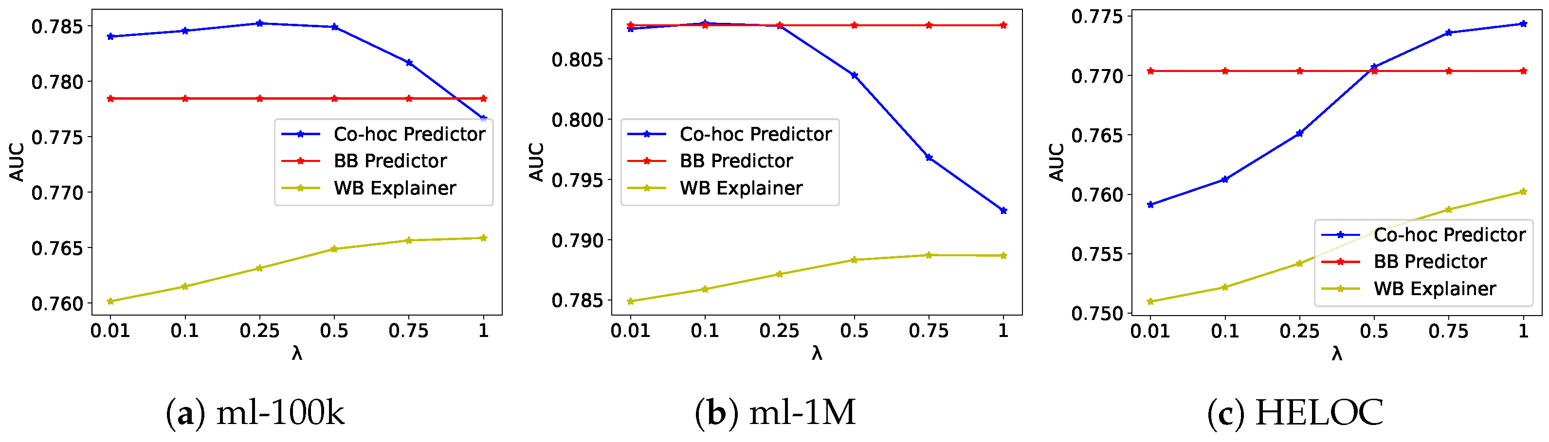
4.1.2. Effect of Regularization Parameter

Figure 1 and Figure 2 illustrate the effect of the explainability regularization parameter ${\lambda }_1$ on the precision and fidelity of our frameworks. As ${\lambda }_1$ increases, we observe a consistent improvement in fidelity scores across all datasets, with only minimal impact on accuracy. This confirms that our frameworks effectively balance the trade-off between accuracy and explainability, allowing users to control this balance through the regularization parameter.

For example, for the ML-100k dataset with the pre hoc framework, as ${\lambda }_1$ increases from 0.01 to 1.0, fidelity improves from 0.8207 to 0.9410 (a 14.6% increase), and accuracy remains relatively stable (0.7840 to 0.7740). Similarly, for the HELOC dataset, fidelity improves from 0.7482 to 0.8454 (a 9.3% increase) as ${\lambda }_1$ increases, with accuracy actually improving slightly from 0.7591 to 0.7719. These results demonstrate that our frameworks can achieve high fidelity without sacrificing accuracy.

The co hoc framework exhibits an even more favorable trade-off curve, particularly in the HELOC dataset, where both accuracy and fidelity improve simultaneously as ${\lambda }_1$ increases. This suggests that the joint optimization approach not only aligns the behavior of the two models but also enhances their complementary strengths. The plateau observed in fidelity scores at higher ${\lambda }_1$ values (above 0.5) indicates an optimal operating point beyond which additional regularization yields diminishing returns. This behavior provides practical guidance for hyperparameter selection in real-world applications, where setting ${\lambda }_1$ between 0.25 and 0.5 offers the best balance between model performance and interpretability.

4.2. Local Explainability Results

Comparison with LIME

Table 2. HELOC Dataset: Comparison with LIME based on neighborhood fidelity and stability results ($\lambda =0.25$, $k=10$). ↑ means higher score is better, ↓ means lower score is better.

Explanation Method	Point Fidelity ↑	Neighborhood Fidelity ↑	Stability ↓
LIME	0.6083 ± 0.0050	0.6600 ± 0.1939	0.2152 ± 0.0175
Pre hoc Framework	0.8270 ± 0.0260	0.9587 ± 0.0766	0.0623 ± 0.0110
Co hoc Framework	0.8300 ± 0.0240	0.9647 ± 0.0575	0.0502 ± 0.0087

presents the comparison of our local explainability frameworks with LIME on the HELOC in terms of point fidelity, neighborhood fidelity, and stability. Both our pre hoc and co hoc local explainability frameworks significantly outperform LIME across all metrics.

On the HELOC dataset, our frameworks achieve neighborhood fidelity scores of 0.9587 (pre hoc) and 0.9647 (co hoc), significantly higher than LIME’s score of 0.6600. Similarly, on the ML-100k dataset, our frameworks achieve neighborhood fidelity scores of 0.9597 (pre hoc) and 0.9647 (co hoc), outperforming LIME’s score of 0.7410. The stability of our explanations, measured by total variation, is also significantly better than LIME, indicating more consistent explanations across different instances.

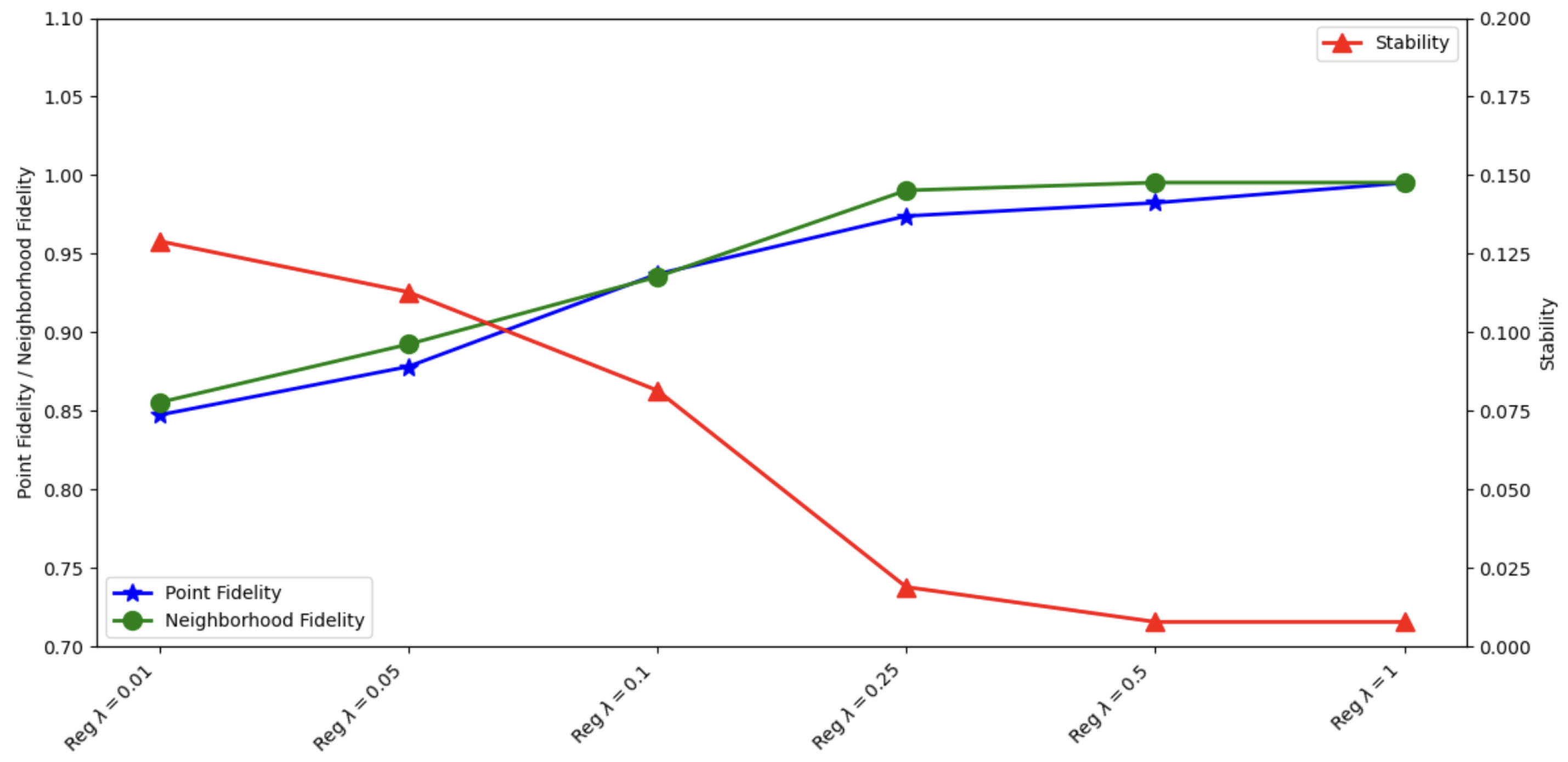
4.3. Effect of Regularization Parameter on Local Explainability Metrics

Table 3. Effect of explainability regularization parameter ${\lambda }_1$ on stability and fidelity for the pre hoc framework on the ML-100k dataset. Comparison of the pre hoc framework with $k=10$, for $\lambda =\{0.01,0.05,0.1,0.25,0.5,1\}$ in point fidelity, neighborhood fidelity, and stability results. “Reg” means that regularization was used. ↑ means higher score is better, ↓ means lower score is better.

Explanation Method	Point Fidelity ↑	Neighborhood Fidelity ↑	Stability ↓
No-regularization	0.8183 ± 0.3524	0.8050 ± 0.1268	0.3524 ± 0.0175
Reg $\lambda =0.01$	0.8473 ± 0.0351	0.8553 ± 0.1158	0.1290 ± 0.0010
Reg $\lambda =0.05$	0.8781 ± 0.0195	0.8923 ± 0.1043	0.1128 ± 0.0009
Reg $\lambda =0.1$	0.9370 ± 0.0230	0.9353 ± 0.0737	0.0815 ± 0.0019
Reg $\lambda =0.25$	0.9740 ± 0.0237	0.9903 ± 0.0329	0.0189 ± 0.0041
Reg $\lambda =0.5$	0.9824 ± 0.0234	0.9953 ± 0.0215	0.0078 ± 0.0010
Reg $\lambda =1$	0.9951 ± 0.0117	0.9953 ± 0.0215	0.0078 ± 0.0010

and Figure 3 show the impact of the explainability regularization parameter ${\lambda }_1$ on the point fidelity, neighborhood fidelity, and stability metrics for the pre hoc framework on the ML-100k dataset. The results show a clear positive relationship between the regularization strength and the quality of the explanation.

In the absence of regularization, the model achieves moderate fidelity scores (point fidelity of 0.8183 and neighborhood fidelity of 0.8050) but exhibits lower stability with a high total variation score of 0.3524. This indicates that without explainability regularization, the explanations are less consistent across different instances, even when the model achieves reasonable alignment with the explainer.

As we train with the regularization parameter and gradually increase the ${\lambda }_1$, we observe significant improvements across all metrics. With a minimal regularization of ${\lambda }_1=0.01$, point fidelity improves to 0.8473 (3.5% increase), neighborhood fidelity increases to 0.8553 (6.2% increase), and stability improves dramatically with total variation decreasing to 0.1290 (63.4% reduction). At ${\lambda }_1=0.25$, point fidelity reaches 0.9740 (19.0% increase from no regularization), neighborhood fidelity increases to 0.9903 (23.0% increase), and stability improves substantially with total variation reduced to 0.0189 (94.6% reduction). This indicates that moderate regularization significantly enhances both the alignment between the predictor and explainer models and the consistency of explanations across different instances.

At higher regularization strengths (${\lambda }_1=0.5$ and ${\lambda }_1=1.0$), the metrics continue to improve but with decreasing returns. The point fidelity reaches its peak at 0.9951 with ${\lambda }_1=1.0$, representing a 21.6% improvement over the non-regularized model. Similarly, neighborhood fidelity reaches 0.9953, a 23.6% improvement. The stability metric plateaus at 0.0078 for both ${\lambda }_1=0.5$ and ${\lambda }_1=1.0$, indicating that additional regularization beyond ${\lambda }_1=0.5$ does not further improve the consistency of explanations.

These results demonstrate that incorporating explainability regularization through the Jensen–Shannon divergence significantly enhances the quality of explanations generated by the pre hoc framework. Even $0.01$ regularization provides substantial benefits, with optimal performance achieved at moderate to high regularization strengths (${\lambda }_1\ge 0.25$). The improvements in fidelity metrics indicate better alignment between the predictor and explainer models, while the reduction in total variation demonstrates more consistent explanations across different instances.

4.3.1. Effect of Neighborhood Size

Table 4. HELOC Dataset: Effect of neighborhood size on neighborhood fidelity, stability, and computation time for the pre hoc framework ($\lambda =0.25$). ↑ means higher score is better, ↓ means lower score is better.

Neighborhood Size	Neighborhood Fidelity ↑	Stability ↓	Computation Time (s)
$k=3$	0.8833 ± 0.1939	0.2152 ± 0.0175	0.0121 ± 0.0014
$k=10$	0.9350 ± 0.0381	0.0505 ± 0.0098	0.0127 ± 0.0009
$k=100$	0.9670 ± 0.0013	0.0015 ± 0.00006	0.0144 ± 0.0061

shows the effect of neighborhood size on neighborhood fidelity, stability, and computation time for the pre hoc framework on the HELOC dataset. As the neighborhood size increases from 3 to 100, neighborhood fidelity improves from 0.8833 to 0.9670, and stability improves from 0.2152 to 0.0015, with only a minimal increase in computation time. This indicates that larger neighborhoods provide more stable and faithful explanations.

4.3.2. Computational Efficiency

Table 5. HELOC Dataset: Computation time comparison for generating explanations on 100 test instances.

Method	Additional Training Time (s)	Avg Explanation Time (s)	Total Time for Single Instance (s)	Total Time for 100 Instances (s)
LIME	-	0.3812 ± 0.0828	0.3812 ± 0.0828	62.580
Pre hoc	5.1020 ± 0.0315	0.0110 ± 0.0015	5.1130 ± 0.0330	6.202
Co hoc	5.3960 ± 0.0330	0.0135 ± 0.0030	5.4095 ± 0.0360	6.746

and

Table 6. ML-100k Dataset: Computation time comparison for generating explanations on 100 test instances.

Method	Additional Training Time (s)	Avg Explanation Time (s)	Total Time for Single Instance (s)	Total Time for 100 Instances (s)
LIME	-	0.4523 ± 0.0912	0.4523 ± 0.0912	45.23
Pre hoc	8.989 ± 0.595	0.0186 ± 0.0013	9.0076 ± 0.5963	10.849
Co hoc	9.383 ± 0.623	0.0211 ± 0.0028	9.4041 ± 0.6258	11.493

compare the computational efficiency of our frameworks with LIME on the HELOC and ML-100k datasets. Although our frameworks include an additional training phase, the average time to generate explanations for individual instances is significantly lower than LIME (0.011s vs. 0.3812s). This efficiency advantage becomes more apparent when generating explanations for multiple instances, with our frameworks being over 20 times faster than LIME for explaining 100 instances. While the additional training overhead is non-trivial, it occurs only during training and is offset by the 30× speedup in explanation generation at inference time compared to LIME. For a model serving 10,000 predictions daily, the training overhead is amortized within hours, making our approach highly practical for production deployments where real-time explanations are required. We observe consistent efficiency advantages across different dataset sizes and domains.

The computational efficiency of our frameworks is particularly advantageous in scenarios where real-time explanations are required or where a large number of instances need to be explained.

4.4. Qualitative Analysis of Explanations

4.4.1. Global Explanations

Figure 4 illustrates the global feature importance scores for the HELOC dataset, providing insights into the overall impact of each feature on the model’s predictions. The most influential feature is MaxDelq2PublicRecLast12M, which measures the maximum delinquency on public records in the last 12 months. This feature negatively impacts credit scores, suggesting that higher delinquency values significantly decrease the likelihood of getting a loan. Similarly, NumTrades90Ever2DerogPubRec, which represents the number of trades with derogatory public records, shows a substantial negative influence on the model’s predictions. This implies that having more trades with derogatory records decreases the probability of the target variable. The global explanation also reveals that features related to credit inquiries and satisfactory trades play a notable role in the model’s decision-making process. MSinceMostRecentInqexcl7days, indicating the time since the most recent credit inquiry, has a positive impact on the predictions, while NumSatisfactoryTrades, which represents the number of satisfactory trades, exhibits a negative influence. This suggests that recent credit inquiries and fewer satisfactory trades are associated with a higher likelihood of the target outcome.

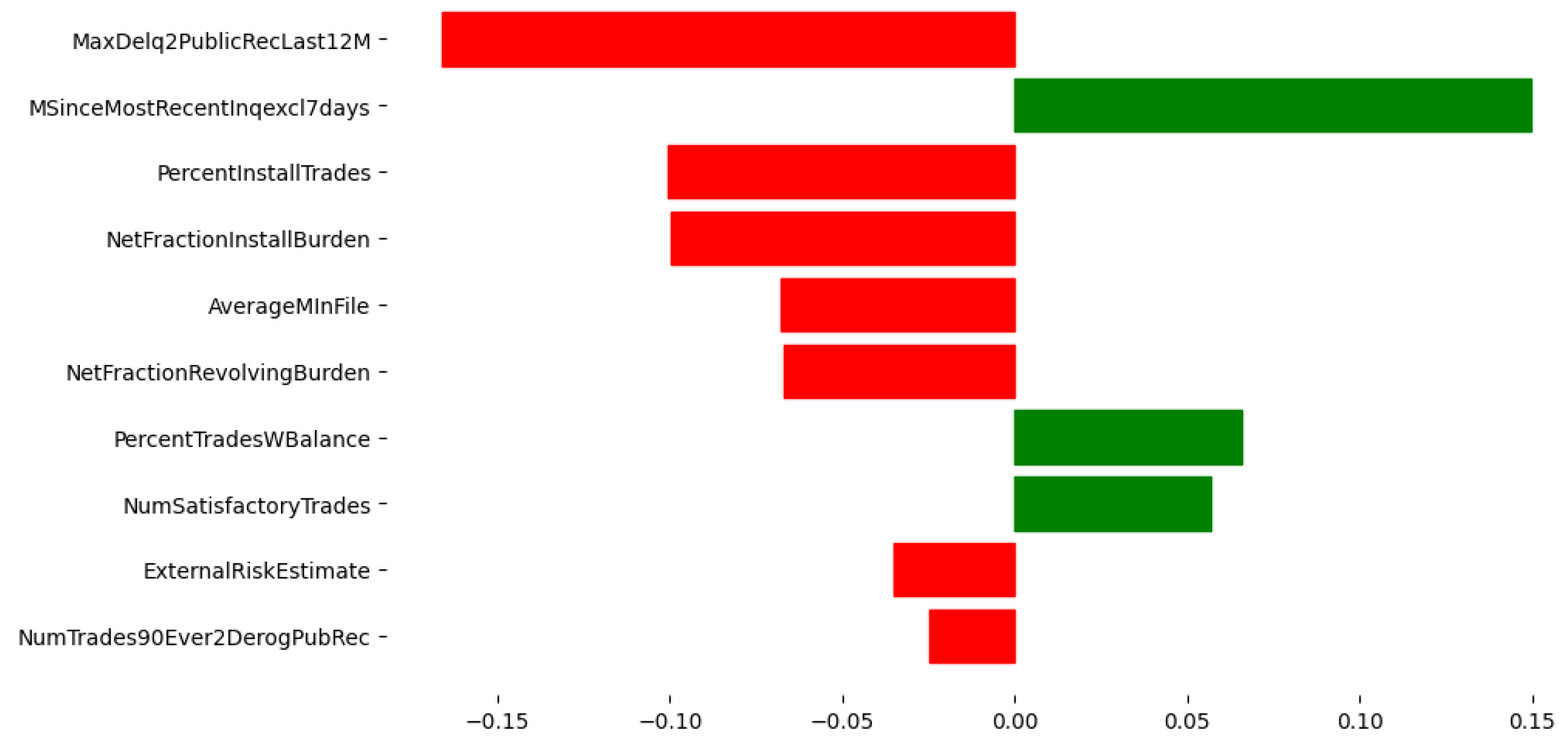
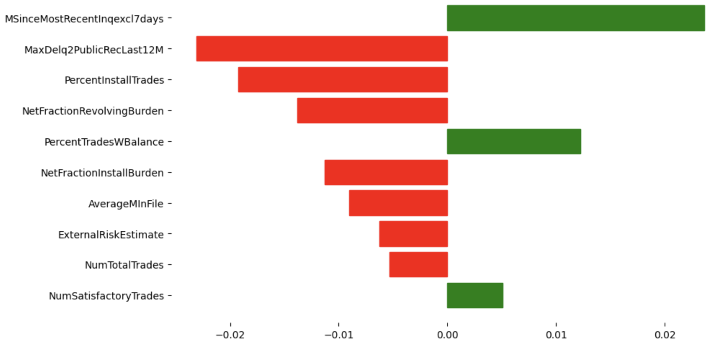
4.4.2. Local Explanations

Figure 5 presents an example of local feature importance scores for a specific test instance from the HELOC dataset. The most influential feature for this instance is MSinceMostRecentInqexcl7days, which has a strong positive impact, indicating that a longer time since the most recent credit inquiry increases the likelihood of the target outcome for this specific instance.

Comparing the local explanation with the global explanation reveals interesting differences. Although both explanations highlight the importance of features such as MaxDelq2PublicRecLast12M and MSinceMostRecentInqexcl7days, the local explanation emphasizes features specific to the instance, such as PercentInstallTrades and NetFractionRevolvingBurden, which may not be as prominent in the global explanation. This shows the value of local explanations in capturing instance-specific factors influencing predictions.

5. Discussion

The performance of our in-training explainability frameworks compared to post hoc methods aligns with recent criticisms of surrogate-based approaches [1,21]. Our fidelity improvements of up to 10.9% support the argument that integrating interpretability during training produces more faithful explanations than post hoc approximation [24]. The computational efficiency gains ($30\times$ faster than LIME) address a critical limitation identified by [17], noting that post hoc methods often introduce prohibitive computational overhead in production systems. Our approach makes real-time explainability feasible for large-scale deployments, similar to the goals outlined in [52] but with significantly lower computational requirements. The stability improvements observed in our experiments (78% reduction in total variation) directly address the consistency concerns raised by [1] regarding LIME’s sensitivity to sampling variations. This stability is crucial for building practitioner trust, as emphasized by [5].

Our finding that explainability constraints can improve model performance confirms recent work on beneficial regularization effects [38], though our approach differs by using an interpretable model as the regularizer rather than explanation-based constraints. Our frameworks address several fundamental challenges identified in the literature on explainability. By integrating the explainer during training rather than approximating it post hoc, we mitigate the surrogate model faithfulness problem that methods like LIME and SHAP face. The black-box model learns to align with interpretable patterns from the start, resulting in explanations that more accurately reflect the model’s actual decision-making process. This approach also eliminates the need for potentially problematic perturbation strategies that can alter feature semantics or produce out-of-distribution samples.

The success of our in-training approach contributes to a paradigm shift in explainable AI, moving from post hoc rationalization to explainability by design. This shift has implications for machine learning workflows and tool development, suggesting that explainability should be considered an objective alongside accuracy during model development. For practitioners in regulated industries or high-stakes applications, our frameworks provide a path to achieving both transparency and performance without the computational overhead associated with post hoc methods. A comprehensive discussion of limitations and future research directions is provided in the following section, Limitations and Future Directions.

Limitations and Future Directions

While our proposed frameworks demonstrate promising results, several limitations warrant consideration. First, a fundamental challenge is the capacity mismatch between simple white-box explainers and complex black-box predictors. When the predictor is significantly more complex (e.g., deep neural networks), the linear explainer may provide oversimplified explanations that miss important non-linear patterns. This gap could limit the fidelity achievable between models of considerably different complexities. Second, our evaluation focuses on Factorization Machines as the black-box model and sparse logistic regression as the explainer. While effective for demonstrating our approach, a comprehensive evaluation with diverse model architectures (deep neural networks) and alternative explainer models (decision trees) can be pursued in future work. Each combination may require different optimization strategies and regularization strengths. Third, we evaluated exclusively on tabular binary classification tasks. Extending our frameworks to other data modalities (images, text, time series) and tasks (multi-class classification, regression) requires careful adaptation of the interpretable model choice and distance metrics. Finally, while we primarily compared our approach with LIME due to its similar local explanation method, a comparison with SHAP was omitted due to methodological differences (Shapley values vs. coefficient-based importance). Future work could explore incorporating game-theoretic concepts from SHAP into our in-training framework.

Despite these limitations, our results on tabular data provide a strong foundation for future extensions. Key research directions include developing theoretical guarantees for the fidelity–accuracy trade-off, exploring alternative explanation types, and adapting the framework to domains where traditional feature-based explanations may not be applicable. As machine learning systems become increasingly utilized in critical applications, approaches that balance between performance and interpretability will be crucial for the responsible deployment of AI.

6. Conclusions

This paper introduces two novel explainability frameworks—pre hoc and co hoc explainability—that integrate interpretability directly into the training process of black-box machine learning models. Unlike post hoc methods that generate explanations after model training, our approach incorporates an inherently interpretable white-box model to guide the learning of the black-box model, ensuring that explanations are faithful to the model’s behavior without compromising accuracy. The pre hoc framework uses a trained white-box explainer model to regularize the black-box predictor model through a fidelity term in the loss function, while the co hoc framework jointly optimizes both models with a shared loss function. Both frameworks leverage the Jensen–Shannon divergence to measure and minimize the discrepancy between the predictions of the two models, ensuring alignment in their behaviors. We further extend these frameworks to provide local explanations by incorporating neighborhood information and developing a two-phase approach: first, training for global fidelity, then generating local explanations through fine-tuning the explainer model within the neighborhood of each test instance. This approach captures the local behavior of the black-box model, providing instance-specific explanations that are more relevant and accurate than global explanations alone.

In conclusion, our pre hoc and co hoc explainability frameworks offer a promising direction for developing machine learning models that are both accurate and transparent. By integrating explainability directly into the training process and extending it to capture local behavior, our approaches address the limitations of post hoc methods and contribute to the advancement of trustworthy and interpretable AI systems.

References

1. Alvarez-Melis, D.; Jaakkola, T.S. On the Robustness of Interpretability Methods. arXiv 2018, arXiv:1806.08049. [Google Scholar] [CrossRef]
2. Adebayo, J.; Gilmer, J.; Muelly, M.; Goodfellow, I.; Hardt, M.; Kim, B. Sanity Checks for Saliency Maps. arXiv 2020, arXiv:1810.03292. [Google Scholar] [CrossRef]
3. Ghorbani, A.; Abid, A.; Zou, J. Interpretation of Neural Networks is Fragile. arXiv 2018, arXiv:1710.10547. [Google Scholar] [CrossRef]
4. Adadi, A.; Berrada, M. Peeking Inside the Black-Box: A Survey on Explainable Artificial Intelligence (XAI). IEEE Access 2018, 6, 52138–52160. [Google Scholar] [CrossRef]
5. Doshi-Velez, F.; Kim, B. Towards a Rigorous Science of Interpretable Machine Learning. arXiv 2017, arXiv:1702.08608. [Google Scholar] [CrossRef]
6. Ribeiro, M.T.; Singh, S.; Guestrin, C. Why should I trust you?: Explaining the predictions of any classifier. In Proceedings of the 22nd ACM SIGKDD International Conference on Knowledge Discovery and Data Mining, San Francisco, CA, USA, 13–17 August 2016; pp. 1135–1144. [Google Scholar]
7. Koh, P.W.; Liang, P. Understanding black-box predictions via influence functions. In Proceedings of the International Conference on Machine Learning, Sydney, Australia, 6–11 August 2017; pp. 1885–1894. [Google Scholar]
8. Lapuschkin, S.; Wäldchen, S.; Binder, A.; Montavon, G.; Samek, W.; Müller, K.R. Unmasking Clever Hans predictors and assessing what machines really learn. Nat. Commun. 2019, 10, 1096. [Google Scholar] [CrossRef]
9. Goodman, B.; Flaxman, S. European union regulations on algorithmic decision-making and a “right to explanation”. AI Mag. 2017, 38, 50–57. [Google Scholar] [CrossRef]
10. Wachter, S.; Mittelstadt, B.; Floridi, L. Why a right to explanation of automated decision-making does not exist in the general data protection regulation. Int. Data Priv. Law 2017, 7, 76–99. [Google Scholar] [CrossRef]
11. Dwork, C.; Hardt, M.; Pitassi, T.; Reingold, O.; Zemel, R. Fairness through awareness. In Proceedings of the 3rd Innovations in Theoretical Computer Science Conference, Cambridge, MA, USA, 8–10 January 2012; pp. 214–226. [Google Scholar]
12. Selbst, A.D.; Barocas, S. The intuitive appeal of explainable machines. Fordham Law Rev. 2018, 87, 1085. [Google Scholar] [CrossRef]
13. Bansal, G.; Wu, T.; Zhou, J.; Fok, R.; Nushi, B.; Kamar, E.; Ribeiro, M.T.; Weld, D. Updates in human-ai teams: Understanding and addressing the performance/compatibility tradeoff. In Proceedings of the AAAI Conference on Artificial Intelligence, Honolulu, HI, USA, 27 January–1 February 2019; Volume 33, pp. 2429–2437. [Google Scholar]
14. Lage, I.; Chen, E.; He, J.; Narayanan, M.; Kim, B.; Gershman, S.; Doshi-Velez, F. An evaluation of the human-interpretability of explanation. arXiv 2019, arXiv:1902.00006. [Google Scholar]
15. Lundberg, S.M.; Lee, S.I. A Unified Approach to Interpreting Model Predictions. In Advances in Neural Information Processing Systems 30; Guyon, I., Luxburg, U.V., Bengio, S., Wallach, H., Fergus, R., Vishwanathan, S., Garnett, R., Eds.; Curran Associates, Inc.: New York, NY, USA, 2017; pp. 4765–4774. [Google Scholar]
16. Selvaraju, R.R.; Cogswell, M.; Das, A.; Vedantam, R.; Parikh, D.; Batra, D. Grad-CAM: Visual Explanations from Deep Networks via Gradient-Based Localization. Int. J. Comput. Vis. 2019, 128, 336–359. [Google Scholar] [CrossRef]
17. Bordt, S.; Finck, M.; Raidl, E.; von Luxburg, U. Post hoc Explanations Fail to Achieve their Purpose in Adversarial Contexts. In Proceedings of the 2022 ACM Conference on Fairness, Accountability, and Transparency, Seoul, Republic of Korea, 21–24 June 2022. [Google Scholar] [CrossRef]
18. Slack, D.; Hilgard, S.; Jia, E.; Singh, S.; Lakkaraju, H. Fooling LIME and SHAP: Adversarial Attacks on Post Hoc Explanation Methods. In Proceedings of the AAAI/ACM Conference on AI, Ethics, and Society, AIES’20, New York, NY, USA, 7–8 February 2020; pp. 180–186. [Google Scholar] [CrossRef]
19. Alvarez-Melis, D.; Jaakkola, T.S. Towards Robust Interpretability with Self-Explaining Neural Networks. arXiv 2018, arXiv:1806.07538. [Google Scholar] [CrossRef]
20. Ghorbani, A.; Wexler, J.; Zou, J.Y.; Kim, B. Towards Automatic Concept-based Explanations. In Advances in Neural Information Processing Systems; Curran Associates, Inc.: New York, NY, USA, 2019; Volume 32. [Google Scholar]
21. Rudin, C. Stop Explaining Black Box Machine Learning Models for High Stakes Decisions and Use Interpretable Models Instead. arXiv 2019, arXiv:1811.10154. [Google Scholar] [CrossRef]
22. Acun, C.; Nasraoui, O. In-Training Explainability Frameworks: A Method to Make Black-Box Machine Learning Models More Explainable. In Proceedings of the 2023 IEEE/WIC International Conference on Web Intelligence and Intelligent Agent Technology (WI-IAT), Venice, Italy, 26–29 October 2023; pp. 230–237. [Google Scholar] [CrossRef]
23. Acun, C.; Ashary, A.; Popa, D.O.; Nasraoui, O. Enhancing Robotic Grasp Failure Prediction Using A Pre hoc Explainability Framework. In Proceedings of the 2024 IEEE 20th International Conference on Automation Science and Engineering (CASE), Bari, Italy, 28 August–1 September 2024; pp. 1993–1998. [Google Scholar] [CrossRef]
24. Laugel, T.; Lesot, M.J.; Marsala, C.; Renard, X.; Detyniecki, M. The Dangers of Post hoc Interpretability: Unjustified Counterfactual Explanations. In Proceedings of the Twenty-Eighth International Joint Conference on Artificial Intelligence, IJCAI-19, International Joint Conferences on Artificial Intelligence Organization, Macao, China, 10–16 August 2019; pp. 2801–2807. [Google Scholar] [CrossRef]
25. Neter, J.; Kutner, M.H.; Nachtsheim, C.J.; Wasserman, W. Applied Linear Statistical Models; Irwin: Chicago, IL, USA, 1996. [Google Scholar]
26. Hosmer, D.W., Jr.; Lemeshow, S.; Sturdivant, R.X. Applied Logistic Regression; John Wiley & Sons: Hoboken, NJ, USA, 2013. [Google Scholar]
27. Quinlan, J.R. Induction of decision trees. Mach. Learn. 1986, 1, 81–106. [Google Scholar] [CrossRef]
28. Breiman, L.; Friedman, J.; Olshen, R.; Stone, C. Classification and Regression Trees; Wadsworth & Brooks/Cole Advanced Books & Software: Monterey, CA, USA, 1984. [Google Scholar]
29. Abdollahi, B.; Nasraoui, O. Explainable matrix factorization for collaborative filtering. In Proceedings of the 25th International Conference Companion on World Wide Web, Montreal, QC, Canada, 11–15 May 2016; pp. 5–6. [Google Scholar]
30. Ras, G.; Ambrogioni, L.; Haselager, P.; van Gerven, M.A.J.; Güçlü, U. Explainable 3D Convolutional Neural Networks by Learning Temporal Transformations. arXiv 2020, arXiv:2006.15983. [Google Scholar] [CrossRef]
31. Fauvel, K.; Lin, T.; Masson, V.; Fromont, É.; Termier, A. XCM: An Explainable Convolutional Neural Network for Multivariate Time Series Classification. arXiv 2020, arXiv:2009.04796. [Google Scholar] [CrossRef]
32. Miao, S.; Liu, M.; Li, P. Interpretable and Generalizable Graph Learning via Stochastic Attention Mechanism. arXiv 2022, arXiv:2201.12987. [Google Scholar] [CrossRef]
33. Tibshirani, R. Regression shrinkage and selection via the lasso. J. R. Stat. Soc. Ser. B Methodol. 1996, 58, 267–288. [Google Scholar] [CrossRef]
34. Hoerl, A.E.; Kennard, R.W. Ridge regression: Biased estimation for nonorthogonal problems. Technometrics 1970, 12, 55–67. [Google Scholar] [CrossRef]
35. Wu, M.; Hughes, M.C.; Parbhoo, S.; Zazzi, M.; Roth, V.; Doshi-Velez, F. Beyond Sparsity: Tree Regularization of Deep Models for Interpretability. In Proceedings of the Thirty-Second AAAI Conference on Artificial Intelligence and Thirtieth Innovative Applications of Artificial Intelligence Conference and Eighth AAAI Symposium on Educational Advances in Artificial Intelligence, AAAI’18/IAAI’18/EAAI’18, New Orleans, LA, USA, 2–7 February 2018; AAAI Press: Washington, DC, USA, 2018. [Google Scholar]
36. Lipton, Z.C. The Mythos of Model Interpretability. arXiv 2017, arXiv:1606.03490. [Google Scholar] [CrossRef]
37. Chen, J.; Song, L.; Wainwright, M.J.; Jordan, M.I. Learning to Explain: An Information-Theoretic Perspective on Model Interpretation. arXiv 2018, arXiv:1802.07814. [Google Scholar] [CrossRef]
38. Ross, A.S.; Hughes, M.C.; Doshi-Velez, F. Right for the Right Reasons: Training Differentiable Models by Constraining their Explanations. In Proceedings of the Twenty-Sixth International Joint Conference on Artificial Intelligence, IJCAI-17, Melbourne, Australia, 19–25 August 2017; pp. 2662–2670. [Google Scholar] [CrossRef]
39. Lee, G.H.; Alvarez-Melis, D.; Jaakkola, T.S. Game-Theoretic Interpretability for Temporal Modeling. arXiv 2018, arXiv:1807.00130. [Google Scholar] [CrossRef]
40. Lee, G.H.; Jin, W.; Alvarez-Melis, D.; Jaakkola, T. Functional Transparency for Structured Data: A Game-Theoretic Approach. In Proceedings of the International Conference on Machine Learning, Long Beach, CA, USA, 9–15 June 2019. [Google Scholar]
41. Plumb, G.; Al-Shedivat, M.; Cabrera, A.A.; Perer, A.; Xing, E.; Talwalkar, A. Regularizing Black-box Models for Improved Interpretability. In Advances in Neural Information Processing Systems; Curran Associates, Inc.: New York, NY, USA, 2020; Volume 33, pp. 10526–10536. [Google Scholar]
42. Sarkar, A.; Vijaykeerthy, D.; Sarkar, A.; Balasubramanian, V.N. A Framework for Learning Ante hoc Explainable Models via Concepts. arXiv 2021, arXiv:2108.11761. [Google Scholar] [CrossRef]
43. Guidotti, R.; Monreale, A.; Ruggieri, S.; Turini, F.; Giannotti, F.; Pedreschi, D. A survey of methods for explaining black box models. ACM Comput. Surv. (CSUR) 2018, 51, 1–42. [Google Scholar] [CrossRef]
44. Letham, B.; Rudin, C.; McCormick, T.H.; Madigan, D. Interpretable classifiers using rules and Bayesian analysis: Building a better stroke prediction model. Ann. Appl. Stat. 2015, 9, 1350–1371. [Google Scholar] [CrossRef]
45. Sundararajan, M.; Najmi, A. Many shapley values. arXiv 2020, arXiv:2002.12296. [Google Scholar]
46. Kim, B.; Wattenberg, M.; Gilmer, J.; Cai, C.; Wexler, J.; Viegas, F.; Sayres, R. Interpretability Beyond Feature Attribution: Quantitative Testing with Concept Activation Vectors (TCAV). In Proceedings of the International Conference on Machine Learning, Stockholm, Sweden, 10–15 July 2018; pp. 2668–2677. [Google Scholar]
47. Bien, J.; Tibshirani, R. Prototype selection for interpretable classification. Ann. Appl. Stat. 2011, 5, 2403–2424. [Google Scholar] [CrossRef]
48. Ribeiro, M.T.; Singh, S.; Guestrin, C. Anchors: High-Precision Model-Agnostic Explanations. In Proceedings of the AAAI Conference on Artificial Intelligence, New Orleans, LA, USA, 2–7 February 2018. [Google Scholar]
49. Van Looveren, A.; Klaise, J. Global aggregations of local explanations for black box models. In Proceedings of the ECML PKDD 2019 Workshop on Automating Data Science, Würzburg, Germany, 16–20 September 2019. [Google Scholar]
50. Caruana, R.; Lou, Y.; Gehrke, J.; Koch, P.; Sturm, M.; Elhadad, N. Intelligible models for healthcare: Predicting pneumonia risk and hospital 30-day readmission. In Proceedings of the 21th ACM SIGKDD International Conference on Knowledge Discovery and Data Mining, Sydney, Australia, 10–13 August 2015; pp. 1721–1730. [Google Scholar]
51. Tonekaboni, S.; Joshi, S.; McCradden, M.D.; Goldenberg, A. What clinicians want: Contextualizing explainable machine learning for clinical end use. In Proceedings of the Machine Learning for Healthcare Conference, Ann Arbor, MI, USA, 8–10 August 2019; pp. 359–380. [Google Scholar]
52. Bhatt, U.; Xiang, A.; Sharma, S.; Weller, A.; Taly, A.; Jia, Y.; Ghosh, J.; Puri, R.; Moura, J.M.; Eckersley, P. Explainable machine learning in deployment. In Proceedings of the 2020 Conference on Fairness, Accountability, and Transparency, Barcelona, Spain, 27–30 January 2020; pp. 648–657. [Google Scholar]
53. Rendle, S. Factorization Machines. In Proceedings of the 2010 IEEE International Conference on Data Mining, ICDM ’10, Sydney, Australia, 13–17 December 2010; pp. 995–1000. [Google Scholar] [CrossRef]
54. Lan, L.; Geng, Y. Accurate and Interpretable Factorization Machines. In Proceedings of the AAAI Conference on Artificial Intelligence, Honolulu, HI, USA, 27 January–1 February 2019; Volume 33, pp. 4139–4146. [Google Scholar] [CrossRef]
55. Anelli, V.W.; Noia, T.D.; Sciascio, E.D.; Ragone, A.; Trotta, J. How to Make Latent Factors Interpretable by Feeding Factorization Machines with Knowledge Graphs. In Lecture Notes in Computer Science; Springer International Publishing: Berlin/Heidelberg, Germany, 2019; pp. 38–56. [Google Scholar] [CrossRef]
56. Xiao, J.; Ye, H.; He, X.; Zhang, H.; Wu, F.; Chua, T.S. Attentional Factorization Machines: Learning the Weight of Feature Interactions via Attention Networks. In Proceedings of the 26th International Joint Conference on Artificial Intelligence, IJCAI’17, Melbourne, Australia, 19–25 August 2017; AAAI Press: Washington, DC, USA, 2017; pp. 3119–3125. [Google Scholar]
57. Nielsen, F.; Boltz, S. The Burbea-Rao and Bhattacharyya Centroids. IEEE Trans. Inf. Theory 2011, 57, 5455–5466. [Google Scholar] [CrossRef]
58. Cover, T.M.; Thomas, J.A. Information theory and statistics. Elem. Inf. Theory 1991, 1, 279–335. [Google Scholar]
59. Hinton, G.; Vinyals, O.; Dean, J. Distilling the knowledge in a neural network. arXiv 2015, arXiv:1503.02531. [Google Scholar]
60. FICO. The FICO HELOC Dataset. Available online: https://www.kaggle.com/datasets/averkiyoliabev/home-equity-line-of-creditheloc (accessed on 15 December 2023).
61. GroupLens. MovieLens 100K Dataset. Available online: https://grouplens.org/datasets/movielens/100k/ (accessed on 15 December 2023).
62. GroupLens. MovieLens 1M Dataset. Available online: https://grouplens.org/datasets/movielens/1M/ (accessed on 15 December 2023).
63. Fawcett, T. An introduction to ROC analysis. Pattern Recognit. Lett. 2006, 27, 861–874. [Google Scholar] [CrossRef]
64. Paszke, A.; Gross, S.; Massa, F.; Lerer, A.; Bradbury, J.; Chanan, G.; Killeen, T.; Lin, Z.; Gimelshein, N.; Antiga, L.; et al. PyTorch: An Imperative Style, High-Performance Deep Learning Library. arXiv 2019, arXiv:1912.01703. [Google Scholar] [CrossRef]
65. Kingma, D.P.; Ba, J. Adam: A Method for Stochastic Optimization. arXiv 2017, arXiv:1412.6980. [Google Scholar] [CrossRef]
Figure 1. Effect of explainability regularization parameter λ 1 on accuracy and fidelity for Pre Hoc Explainability Framework on the ml-100k (a), ml-1M (b), and HELOC (c) datasets. The pre hoc predictor is our proposed model, BB is the original black-box predictor model, and WB is the explainer model.
Applsci 15 07544 g001
Figure 2. Effect of explainability regularization parameter λ 1 on accuracy and fidelity for Co Hoc Explainability Framework on the ml-100k (a), ml-1M (b), and HELOC (c) datasets. The co hoc predictor is our proposed model, BB is the original black-box predictor model, and WB is the explainer model.
Applsci 15 07544 g002
Figure 3. Effect of explainability regularization parameter λ 1 on point fidelity, neighborhood fidelity, and stability for the pre hoc framework on the ML-100k dataset results. Comparison of the pre hoc framework with k = 10 , for λ = { 0.01 , 0.05 , 0.1 , 0.25 , 0.5 , 1 } .
Applsci 15 07544 g003
Figure 4. HELOC Dataset: Top 10 Feature Importance scores from the global explanation of the pre hoc framework. Red color means negative contribution, green color means positive contribution on features.
Applsci 15 07544 g004
Figure 5. HELOC Dataset: Local explanation for a test instance, showing the top 10 feature importance scores. Red color means negative contribution, green color means positive contribution on features.
Applsci 15 07544 g005