The Simulation of Grouting Behavior in the Pea Gravel Filling Layer Behind a Double-Shield TBM Based on the Level Set Method

Abstract

In double-shield TBM tunnel construction, grouting plays a vital role in consolidating the gravel backfill and maintaining the integrity of the segmental lining. To investigate the permeation behavior of grout within the pea gravel layer, a fluid dynamics model was developed in this study. The model directly simulates the flow of grout through the porous medium by solving the Navier–Stokes equations and employs the level set method to track the evolving interface between the grout and air phases. Unlike conventional continuum approaches, this model incorporates particle-scale heterogeneity, allowing for a more realistic analysis of grout infiltration through the non-uniform pore structures formed by gravel packing. Three different grouting port positions and two boundary conditions are considered in the simulation. The results indicate that under pressure boundary conditions, the grout flow rate increases rapidly in the initial stage, and then decreases and stabilizes, with the flow rate peak increasing as the grout port moves upward. Under velocity boundary conditions, the injection pressure grows slowly in the early stage but accelerates with time. Additionally, the rate of pressure change is faster when the grout port is located lower in the backfilling layer. Through theoretical analysis, the existing analytical formula was extended by introducing a gravitational correction term. When the grouting port is near the upper part of the tunnel, the analytical solution aligns well with the numerical simulation results, but as the grout port moves downward, the discrepancy between the two increases.

1. Introduction

With the development of urban underground space, double-shield tunnel boring machines (TBMs) are increasingly applied in various tunnel construction projects due to their advantages, such as minimal impact on the surrounding environment, fast construction progress, and the ability to handle complex geological conditions [1,2,3,4]. Synchronous grouting, as an environmental protection and tunnel stability control technique, plays a crucial role in double-shield TBM construction [5,6,7]. However, due to the unpredictable conditions behind the segmental lining, issues such as grout blockage and insufficient grouting are common during the synchronous grouting process. Therefore, exploring the flow mechanisms of grout has become an important research issue that needs to be addressed in double-shield TBM tunnel construction.

Currently, the common methods used to study the permeability of grouts include theoretical analytical solutions [8,9], physical model experiments [10,11], and numerical research [12,13]. Mittag and Savidis [14] conducted laboratory experiments to investigate the permeability of microfine cement grouts in sandy soils and analyzed the impact of particle size on grout permeability. Maghous et al. [15] derived a macroscopic model for grouting permeability in porous media based on mass balance equations for different components in the grouting medium and the general phenomenological filtration law. Eklund and Stille [16] investigated the effect of the specific surface area of particles on the permeability of grout. The results indicated that finer cement particles have a higher specific surface area and, consequently, a higher surface charge, leading to lower grout permeability. Axelsson et al. [17] analyzed the stopping mechanism of grout during permeation grouting under different water-to-cement ratios through laboratory sand column experiments combined with field grouting. Lee et al.’s [18] experiments showed that adding oscillatory pressure to the steady-state injection pressure can reduce the adhesion of cement particles, thus improving grouting efficiency. Weng et al. [19] conducted a series of permeability grouting experiments on fractured sandstone samples using low-field nuclear magnetic resonance (LF-NMR) technology, investigating the grout injection volume, effective grouting time, and grout filling velocity under different grouting conditions. Wang et al. [20], based on fractal theory, considered the tortuosity of porous media and the time-dependent viscosity behavior of grout, and derived a two-stage column–hemispherical diffusion model of Newtonian fluid. However, most of these studies employed simplified models of porous media, homogenizing the porous structure and neglecting the influence of the microstructure of the porous medium on grout flow.

Many scholars have considered factors such as fluid type and grout viscosity, and developed a variety of analytical models to study grout diffusion patterns under different conditions. Gou et al. [21] treated the shield tail void as a three-dimensional circular thin cake and derived models for the grout filling pressure distribution along the circumferential direction of the shield tail gap under both Newtonian and Bingham fluid conditions. Ye et al. [22] considered the interaction between soil pores and grouting, and developed a hemispherical surface diffusion model to determine the grouting pressure based on soil porosity. Liu et al. [23], based on the characteristics of quasi-rectangular shield tunnels, took into account the viscous resistance during grout filling and diffusion, and derived a three-dimensional spatial distribution model for the diffusion pressure of synchronous grouting in quasi-rectangular shield tunnels. Ma et al. [24] investigated the circumferential, longitudinal, and radial distribution characteristics of grout pressure and developed a pressure distribution and dissipation model that accounts for the time-dependent viscosity of Bingham grout. However, most of the above studies provide steady-state analytical solutions for grout pressure distribution, lacking an analysis of the grout diffusion process.

In this study, the level set method is employed to simulate the interface evolution between grout and air. Through the integration of the discrete element method (DEM) with the finite element method (FEM), a heterogeneous pore structure model of the pea gravel backfill layer is constructed. The grout infiltration behavior within the backfilling layer during the injection process is systematically analyzed, addressing a research gap in the numerical simulation of grout infiltration in the backfill layer of double-shield TBM projects. This study implemented grout injection using both pressure boundary conditions and velocity boundary conditions, obtaining the permeability characteristics of grout within gravel pores and pressure distribution patterns. Building upon previous research, the basic principles of fluid mechanics and the limit equilibrium method are used to establish a mathematical model for synchronous grouting in shield tunnel construction. An expression for grouting pressure is derived and compared with the simulation results to verify the reliability of the model.

2. Numerical Model for Grout Permeability in Backfilling Layers

2.1. Modeling Strategy and Computational Methods

To systematically investigate the grout diffusion process within the pea gravel layer of a double-shield TBM tunnel, a heterogeneous porous media infiltration model was established in this study. The simulation methodology and workflow are presented in Figure 1. The modeling process integrates two software platforms: PFC 5.0 and COMSOL 6.2. The objectives of employing PFC are twofold: (1) to approximate the porosity of the pea gravel layer by simulating its consolidation process; and (2) to generate discrete particles for the construction of a porous media model. On this basis, a porosity model of the pea gravel layer is developed in COMSOL.

The grouting process is treated as a two-phase flow problem involving grout and air. The interface between the two phases is tracked using the level set method, which enables the precise capture of the evolving grout–air boundary. A transient solver is employed to simulate the time-dependent behavior of interface propagation and grout diffusion within the complex pore structure.

The motion of the grout is governed by the Navier–Stokes equations, which express the fundamental laws of momentum conservation. The incompressible form of the Navier–Stokes equations used to describe the two-phase flow is as follows:

$$\rho \left[{\displaystyle \frac{\partial u}{\partial t}}+(u\cdot \nabla )u\right]=\nabla \left[-pI+\mu (\nabla u+\nabla u^T)\right]+F$$

(1)

$$\nabla u=0$$

(2)

where ρ represents the fluid density, u denotes the velocity field of the fluid, p is the pressure, μ is the dynamic viscosity, I is the identity tensor, and F accounts for external forces acting on the fluid.

To model the dynamic interface between two phases (grout and air), the level set method is utilized. This method captures the movement of the interface by solving the following equation:

$${\displaystyle \frac{\partial \varphi }{\partial t}}+u\cdot \nabla \varphi =\nabla \cdot \left[\epsilon \nabla \varphi -\varphi \left(1-\varphi \right){\displaystyle \frac{\nabla \varphi }{\left|\nabla \varphi \right|}}\right]$$

(3)

where ϕ represents the level set function, and ε is the thickness control parameter. The value of ϕ varies between 0 and 1 and can represent the volume fraction of the two phases. When ϕ = 0, the fluid is in the gas phase; when ϕ = 0.5, the fluid is in the liquid phase. When 0 < ϕ < 1, ϕ represents the phase interface with a certain thickness. In post-processing, the iso-surface of ϕ = 0.5 is typically taken as the phase interface.

2.2. Construction of the Numerical Model

The segments are assembled inside the shield machine and then pushed out through the shield tail. An annular gap is formed between the surrounding rock and the segmental lining, which is typically filled with gravel first, followed by grout injection. The grout bonds the gravel, surrounding rock, and segmental lining into an integrated structure, forming a complete backfilling layer (Figure 2a) that serves to transmit the surrounding rock pressure and provide impermeability.

The pea gravel used in the project typically consists of two types—natural pebbles and artificial crushed stones (Figure 2b)—with particle sizes generally ranging from 5 × 10⁻³ m to 1 × 10⁻² m. Natural pebbles are sourced from riverbeds, and their surfaces are smooth and rounded; artificial crushed stones are produced by breaking rocks, resulting in rougher surfaces with sharp edges. After being blown into the gap, the gravel accumulates and fills the void, forming the backfilling layer. The gravel backfilling layer is a typical porous medium. Compared to other porous media, the gravel backfilling layer has larger pore sizes and better connectivity between the pores.

To estimate the porosity of the pea gravel layer, the filling process of gravel particles was simulated using PFC. First, randomly distributed particles are generated within a cubic region, with particle sizes uniformly distributed between 5 × 10⁻³ m and 1 × 10⁻² m. Then, a pressure of 1 MPa is applied in all directions to compact the particle packing, transforming it from a loose to a dense configuration and thereby eliminating excess voids. The number of particles generated in this simulation is 827. The particle density is 2500 kg/m³, with the contact stiffness of particles set to 4 × 10⁷ N/m and contact stiffness of the walls set to 2 × 10⁸ N/m. The friction coefficient is 0.6, and the damping ratio is 0.7. The particle generation and consolidation results are shown in Figure 3, with the overall porosity being approximately 0.4.

From the grouting port, the grout can flow in three directions: circumferential, axial, and radial. Therefore, the diffusion of grout within the backfilling layer is a complex three-dimensional problem. However, in this study, the grout flow is only considered in the circumferential direction for the following three reasons:

• Both segmental lining and surrounding rock can be treated as impermeable layers.
• The circumferential diffusion speed of the grout is generally much greater than the axial diffusion speed in engineering applications [24].
• The circumferential perimeter of the backfilling layer is significantly larger than its thickness and axial length, making circumferential diffusion the dominant mode of grout flow.

The simplified backfilling layer is an annular region with an inner diameter of 2 m and an outer diameter of 2.4 m. Since the grouting positions in tunnel construction are symmetrically distributed on the left and right sides, this study analyzes only the left half of the annular region.

The process of constructing the backfilling layer computational model is shown in Figure 4. The first step is to generate a discrete set of particles using discrete element software. Due to computational resource limitations, this study scaled up the size of the gravel particles when constructing the porous medium model. Based on the results of the particle packing simulation mentioned earlier, the porosity at the time of particle generation is set to 0.4, with particle diameters ranging from 0.02 to 0.04 m.

The second step involves importing the particle set data into COMSOL. The built-in functions in PFC (Particle Flow Code) allow the convenient retrieval of data such as the radius and coordinates of each particle. MATLAB R2024b is used to read the exported particle data, and the particles are re-plotted in COMSOL.

The third step applies Boolean operations to remove particles while preserving the pores between them, resulting in a geometric model of the pores in the backfilling layer.

The fourth step is to convert the obtained pore geometric model into a mesh, which will be used for the subsequent simulation in COMSOL. The generated mesh consists entirely of triangular elements, with a maximum mesh size of 0.02 m and a minimum mesh size of 5.6 × 10⁻⁵ m.

In this study, two fluid materials, air and grout, were used. The relevant material parameters are shown in

Table 1. Calculation parameters.

Density of Air	Viscosity of Air	Density of Grout	Viscosity of Grout
1.204 kg/m3	1.81 × 10−5 Pa·s	1500 kg/m3	0.01 Pa·s

. The material parameters for air were set based on the physical properties under standard atmospheric pressure and a temperature of 20 °C, while the material parameters for cement mortar were based on the experimental data of Rosquot et al. [25].

All the pores are initially filled with air. A small portion of initial fluid elements is created near the entrance as the grout pipe, which is initially filled with grout. Since the model is annular, the azimuth angle can conveniently represent positional information. Therefore, in the following sections of this study, the position descriptions are expressed using the angle α. The values of α corresponding to the grouting port are 30°, 90°, and 150°, as shown in Figure 5a.

Figure 5b shows the setup of the fluid boundary conditions. The boundary condition at the fluid outlet is set as a pressure boundary condition with the pressure value set to zero. Two boundary condition schemes are considered at the inlet:

• Pressure Boundary Condition: A fixed pressure is applied at the inlet.
• Flow Velocity Boundary Condition: A constant flow velocity is applied at the inlet.

Subsequently, the transient solver with default parameters was used to perform the simulation.

The fluid exists only within the pores, with the particle boundaries set as impermeable and no-slip boundary conditions applied at the particle contours. As shown in Figure 5c, the generated porous medium model contains areas that are not connected to other regions, and these areas do not contribute to fluid exchange. Therefore, they are excluded from the model.

3. Analysis of Results

3.1. Diffusion Behavior

Figure 6 illustrates the grout diffusion distance at different time points. The grouting port is positioned at 90°, and the boundary condition at the fluid outlet is a pressure boundary condition. In the figure, the blue region (ϕ = 1) represents grout, while the red region (ϕ = 0) represents air. The interface between the cement mortar and air forms a transition zone (0 < ϕ < 1), which is depicted in green and yellow in the figure.

At the beginning of grouting, the transition zone is relatively short, and the interface between the grout and air is well-defined. As the grout continues to diffuse, the interface becomes irregular, and the transition zone extends.

Figure 7 illustrates the variation in grout diffusion distance over time when the grouting port is positioned at 30° and 150°. Due to the influence of gravity, the downward diffusion velocity of the grout is higher than the upward diffusion velocity. Additionally, during downward diffusion, the interface between the grout and air is irregular, resulting in a longer transition zone. In contrast, during upward diffusion, the interface is well-defined, and the transition zone remains shorter.

Figure 8 illustrates the grout flow in a specific region of the backfilling layer when the grouting port is positioned at 90° and the grouting time reaches 3 s. This region is located above the grouting port, with its exact position marked by the red dashed line in Figure 6. Figure 8a presents the fluid pressure contour map, where the fluid pressure gradually decreases along the direction of grout diffusion. Regions with a larger pressure drop gradient are typically found in narrow particle gaps, whereas in larger pores, the pressure distribution is more uniform.

Figure 8b is the fluid velocity contour map, where regions with higher flow velocity exhibit a slender, tubular distribution. Due to the highly heterogeneous nature of the pore space, certain regions with larger pores and better connectivity serve as primary flow channels, allowing the fluid to preferentially flow through these pathways. As a result, elongated high-velocity regions are formed.

3.2. Pressure Boundary Conditions

Figure 9 shows the variation in the grout diffusion distance over time. The horizontal axis represents the azimuth angle corresponding to the measurement points, while the vertical axis represents the volume fraction of grout. At t = 0 s, grouting begins, and at this time, except for the grouting port, all measurement points have a ϕ value of 0, indicating that the pores are completely filled with air.

At t = 0.6 s, the ϕ value near the grouting port approaches 1, indicating that the voids near the grouting port have been completely filled with grout. Between t = 1.2 s and t = 2.4 s, the curve as a whole moves toward the straight line ϕ = 1, meaning that the grout gradually fills the gaps.

At t = 3 s, the ϕ value at most locations reaches 1. Only at the starting and ending positions does ϕ remain between 0 and 1, indicating that the grout has diffused throughout the entire backfilling layer. However, small amounts of air still remain at the top and bottom of the tunnel. This behavior suggests that while the grout has filled the majority of the backfilling layer, some air pockets remain in the less accessible regions.

Figure 10 illustrates the dissipation of grouting pressure within the gravel backfilling layer. The phase interface is defined at ϕ = 0.5, and its position is indicated by a dashed line in Figure 10. The highest pressure occurs at the grouting port, and the pressure gradually decreases from the grout inlet to the grout outlet, eventually approaching 0 kPa, in line with the expected boundary condition.

As shown in Figure 10a, when the grout injection port is located at the 30° position, the dissipation process of the injection pressure can be divided into two parts—from 0° to 30° and from 30° to 180°—with the injection port serving as the boundary. In the 0° to 30° range, the grout diffuses toward the upper outlet. Due to its proximity to the fluid outlet and the short distance traveled, the pressure dissipates quickly, with the pressure change following a nearly linear trend. In the 30° to 180° range, the grout diffuses toward the lower outlet. Since this part of the grout is farther from the fluid outlet and must travel a greater distance through a large volume of the porous medium, the dissipation of fluid pressure is slower, resulting in a more gradual pressure change.

The distribution of fluid pressure corresponds to the distance over which the grout diffuses, with the fluid pressure typically decreasing to zero at the interface between the grout and air. Figure 10a illustrates the diffusion of grout when the injection port is at the 30° position. At this point, the grout primarily diffuses downward, and the diffusion speed remains relatively steady. Every 0.6 s, the interface between the grout and air moves downward by approximately 20°. For instance, at 0.6 s, the fluid pressure drops to zero at the 90° position, and the grout has diffused to the 100° position; at 1.2 s, the pressure drops to zero at the 120° position, and the grout has diffused to the 130° position. Notably, when the injection port is positioned at 150° (Figure 9c), the grout primarily diffuses upward. In this case, the grout initially maintains the same diffusion speed, but the rate of diffusion slows down in the later stages.

Figure 11 shows the variation in the grout flow rate under pressure boundary conditions. In the initial stage (0 to 0.2 s), the flow rate rises rapidly and reaches its peak at t = 2 s. The peak value is highest when the grouting port is at 30°, reaching 0.251 m²/s, while the peak values at 90° and 150° are lower, at 0.177 m²/s and 0.185 m²/s, respectively. In the middle stage (0.2 to 1 s), the flow rate decreases rapidly. The decrease is most significant when the grouting port is at 30°, dropping to approximately 0.160 m²/s, whereas the flow rate decline is less pronounced at 90° and 150°. In the later stage (1 to 3 s), the flow rate stabilizes. When the grouting port is at 30° and 90°, the flow rates are equal and remain higher than the flow rate at 150°.

This phenomenon can be explained as follows: In the initial stage, cement grout is injected into the porous medium under high pressure. Since the pores of the medium are not yet fully filled, the resistance is relatively low, leading to a rapid increase in the flow rate. As the injection progresses, the cement grout gradually fills the pores, causing an increase in permeability resistance, which results in a decrease in the flow rate until it stabilizes.

When the grouting port is at 90°, the flow rate exhibits relatively small variations, indicating that the permeability of the pore structure in this region is more uniform. In contrast, when the grouting port is at 150°, the flow rate fluctuates more significantly, which may suggest that the pore structure near the grouting port is denser or that local clogging has occurred.

3.3. Velocity Boundary Conditions

With a boundary condition of v = 0.2 m/s, the grout diffusion and pressure dissipation are shown in Figure 12 and Figure 13. In this case, the flow rate of the grout is 0.04 m²/s, which is approximately one-quarter of the flow rate achieved under the pressure boundary condition when it stabilizes.

As shown in Figure 12b, at t = 2 s, the grout volume fraction at the 110° position is 0.935, indicating that the grout has completely filled the pores at this location. In contrast, at the 70° position, the grout volume fraction is only 0.119, indicating that only a small amount of grout exists in the pores at this location. The grout is diffusing downward faster than upward. This phenomenon is also observed under pressure boundary conditions, and it is likely due to the slower injection speed in the pressure boundary case, which results in a more pronounced difference in diffusion speed under the velocity boundary condition.

The pressure at the grouting port increases gradually over time, and the lower the position of the grouting port, the higher the pressure. When the grouting port is at 30°, the maximum pressure is 16.9 kPa, while at 150°, the maximum pressure reaches 31.5 kPa, approximately twice the value at 30°. Additionally, when grouting takes place at 150°, the pressure increases at a relatively steady rate, while in other cases, the pressure growth rate accelerates over time.

Figure 14 illustrates the variation in grouting pressure under the velocity boundary condition. From 0 to 0.5 s, the grouting pressure remains nearly constant, as a large number of pores in the backfilling layer have not yet been filled, resulting in low resistance to grout flow. As time progresses, the grouting pressure gradually increases. The lower the position of the grouting port, the faster the pressure increases, indicating that greater resistance is encountered during grout diffusion at lower positions. From 1.7 to 2 s, the grouting pressure at 30° and 90° suddenly increases, possibly because the grout has diffused into narrower pore regions, where the obstruction of grout movement leads to a rise in pressure.

4. Analytical Formula for Grouting Pressure

Zhou [26] established a grouting pressure model for porous media under the assumption of linear grout flow paths. In this study, the model is extended to the circumferential direction to represent grout infiltration within the annular pea gravel backfilling layer.

To verify the validity of the numerical model, theoretical analysis was conducted, and an analytical solution for the grouting pressure was proposed. The gravel layer is regarded as a bundle of capillaries. The equivalent width b of the porous medium can be estimated, and the calculation formula is as follows:

$$b={\displaystyle \frac{e\cdot b_0}{k\cdot \Sigma C/l}}$$

(4)

where e is the porosity of the porous medium, b₀ is the width of the pea gravel layer, ∑C is the specific surface area per unit area, defined by the perimeter of all particles, l is the length of the fluid domain, and k is an empirical parameter affected by the particle distribution, which is set to 2.7 in this calculation. The calculation results of the equivalent width b of the numerical model in this study are shown in

Table 2. Calculation results of the equivalent width.

Sum of Grain Perimeter	Length of Fluid Domain	Width of Fluid Domain	Equivalent Width
55.414 m	3.456 m	0.2 m	0.00185 m

.

Taking a fluid element within the capillary tube for force analysis, as shown in Figure 15, the force balance equation is

$$2\tau \mathrm{d}l+2h\mathrm{d}p=0$$

(5)

Therefore, the distribution of the shear stress on the fluid element is given by

$$\tau =-h{\displaystyle \frac{\mathrm{d}p}{\mathrm{d}l}}$$

(6)

The velocity distribution of the grout is given by [27]

$$v=\left\{\begin{array}{cc}{\displaystyle \frac{1}{\mu }}\left[-{\displaystyle \frac{b^2-4h^2}{16}}{\displaystyle \frac{dp}{dl}}-{\tau }_0(b/2-h)\right]& (h_0\le h\le b)\\ {\displaystyle \frac{1}{\mu }}\left[-{\displaystyle \frac{b^2-4h_0^2}{16}}{\displaystyle \frac{dp}{dl}}-{\tau }_0(b/2-h_0)\right]& (h\le h_0)\end{array}\right.$$

(7)

$$h_0=-{\tau }_0{\left({\displaystyle \frac{dp}{dl}}\right)}^{-1}$$

(8)

τ₀ is the yield shear stress, which is set to 7 Pa. The average velocity is expressed as

$$\overline{v}={\displaystyle \frac{1}{b}}{\displaystyle {\int }_{-b/2}^{b/2}v}\mathrm{d}h$$

(9)

By substituting into Equation (7), we can obtain

$$\overline{v}={\displaystyle \frac{b^2}{12\mu }}\left[-{\displaystyle \frac{dp}{dl}}-3\lambda -4{\displaystyle \frac{{\lambda }^3}{{\left(dp/dl\right)}^2}}\right],\lambda ={\displaystyle \frac{{\tau }_0}{b}}$$

(10)

Since dp/dl is much larger than λ, the last term in the parentheses can be omitted, and the equation can be directly integrated. When the grouting velocity is constant, the relationship between v and l can be expressed as Equation (11) based on the principle of mass conservation:

$$l={\displaystyle \frac{vt}{e}}$$

(11)

Through integrating Equation (10) and substituting Equations (4) and (11), the relationship between grouting pressure and grouting time can be obtained:

$$p=\left(12\mu v{\left({\displaystyle \frac{k\cdot \Sigma C/l}{e\cdot b}}\right)}^2+3{\tau }_0{\displaystyle \frac{k\cdot \Sigma C/l}{e\cdot b}}\right)\cdot {\displaystyle \frac{vt}{e}}$$

(12)

Assuming that the grout diffuses at the same velocity in both directions, the velocity v in Equation (12) should be taken as half of the injection speed. The grout column formed after a certain period is shown in Figure 16.

Given that β = α − θ/2, the result can be derived using trigonometric functions:

$$h_g=2R\cos ({\displaystyle \frac{\pi }{2}}-{\displaystyle \frac{\theta }{2}})\sin (\alpha -{\displaystyle \frac{\theta }{2}})$$

(13)

When considering the self-weight of the grout, if it is assumed that the gravitational pressure at point M is equal to that at the injection port, then the pressure at the injection port caused by the upward-diffusing grout column can be expressed as

$$p_g=2\rho \mathrm{g}R\cos ({\displaystyle \frac{\pi }{2}}-{\displaystyle \frac{\theta }{2}})\sin (\alpha -{\displaystyle \frac{\theta }{2}})$$

(14)

where θ can be calculated from Equation (11):

$$\theta ={\displaystyle \frac{l}{R}}={\displaystyle \frac{vt}{eR}}$$

(15)

Equation (14) can be written as

$$p_g=2\rho \mathrm{g}R\cos ({\displaystyle \frac{\pi }{2}}-{\displaystyle \frac{vt}{2eR}})\sin (\alpha -{\displaystyle \frac{vt}{2eR}})$$

(16)

By adding Equations (16) and (12), the following can be obtained:

$$\begin{array}{l}p=\left(12\mu v{\left({\displaystyle \frac{k\cdot \Sigma C/l}{e\cdot b}}\right)}^2+3{\tau }_0{\displaystyle \frac{k\cdot \Sigma C/l}{e\cdot b}}\right)\cdot {\displaystyle \frac{vt}{e}}\\ +2\rho \mathrm{g}R\cos ({\displaystyle \frac{\pi }{2}}-{\displaystyle \frac{vt}{2eR}})\sin (\alpha -{\displaystyle \frac{vt}{2eR}})\end{array}$$

(17)

Based on the proposed formula, the grouting pressure can be estimated using the given parameters. The estimated results are compared with the numerical results, as shown in Figure 17, where the solid line represents the numerical simulation results, and the dashed line represents the results estimated by the formula. At the initial stage of grouting, the pressure value obtained from the formula is slightly higher than the simulated value. When the grouting port is at 30°, the dashed line is closer to the solid line. In contrast, when the grouting port is at 150°, there is a significant difference between the dashed and solid lines. At t = 2 s, the formula-calculated value is only 40% of the simulated value.

The analytical formula for grouting pressure developed in this study represents an extension of existing theoretical models and provides a preliminary analysis of pressure variations in pea gravel backfill layers. However, several limitations remain. First, in practical engineering applications, the grouting velocity is typically variable rather than constant, indicating that the formula should be modified to better reflect real-world conditions. Second, the formula does not account for the dynamic variation in grout viscosity over time or with flow conditions, which may compromise its accuracy during long-duration or large-volume grouting operations. Additionally, the current formula was derived under two-dimensional assumptions and neglects the axial diffusion of the grout; thus, its applicability and accuracy in three-dimensional contexts require further investigation and validation.

To investigate the influence of porosity variation in the filling layer on grouting performance, two new pore structure models were constructed with porosities of 0.3 and 0.5, respectively. In both models, the grouting port was positioned at α = 150°, with the corresponding sums of grain perimeters being 65.168 m for the 0.3-porosity model and 49.201 m for the 0.5-porosity model.

Figure 18 presents the time-dependent grouting pressure curves for the models with porosities of 0.3 and 0.5. The numerical simulation results indicate that the grouting pressure in both models exhibits an approximately linear increase over time. Specifically, the simulated pressure values for the 0.3-porosity model are consistently higher than the predicted values, with the predicted value at 2 s being approximately 65% of the simulated result. In contrast, the simulated values for the 0.5-porosity model show a higher degree of agreement with the theoretical predictions. Moreover, the pressure in the 0.3-porosity model increases at a faster rate than in the 0.5-porosity model, indicating that a lower porosity leads to greater resistance during grouting and thus results in higher pressure development.

To analyze the influence of grout injection velocity on grouting performance, two additional models were constructed with injection velocities set to 0.1 m/s and 0.3 m/s, respectively. In both models, the grouting port was positioned at α = 150°. Figure 19 presents the time-dependent grouting pressure curves under the two injection velocity conditions. The numerical simulation results demonstrate that an increase in injection velocity leads to a significant rise in grouting pressure. Moreover, as the injection velocity increases, the discrepancy between the simulated and predicted pressure values becomes more pronounced. This indicates that the theoretical formula is more suitable for predicting grouting behavior at lower injection velocities, whereas its accuracy diminishes as the injection speed increases.

To investigate the influence of grout viscosity on grouting performance, two additional models were developed with grout viscosities set to 0.007 Pa·s and 0.02 Pa·s, respectively. In both models, the grouting port was positioned at α = 150°. Figure 20 presents the time-dependent grouting pressure curves for the two viscosity conditions. The results show that an increase in grout viscosity leads to a corresponding increase in grouting pressure. Furthermore, both the simulated and predicted pressure values for the 0.02 Pa·s model are approximately twice those observed in the 0.007 Pa·s model, indicating that grout viscosity has a significant impact on pressure development during the grouting process.

To validate the reliability of the simulation results, two sets of laboratory grouting experiments conducted by Zhu [28] and Zhang [29] were introduced for comparative analysis. In both experiments, a constant grout injection rate was applied, and the variation in grouting pressure over time was recorded, as shown in Figure 21. The red line represents the results from Zhu’s experiment, in which the water–cement ratio of the grout was 1.5, the sand particle size ranged from 0.05 to 1.2 mm, and the injection rate was 2.85 L/min. The blue line corresponds to Zhang’s experiment, where the grout had a water–cement ratio of 1.1, the sand particle size ranged from 1 to 2 mm, and the injection rate was 4 L/min. Under conditions of constant grout injection velocity, the grouting pressure exhibits an approximately linear increase over time, which aligns well with the trend observed in the present study. Additionally, the particle size range of the granular medium appears to have a significant impact on the grouting pressure response, indicating a need for further investigation into its influence.

5. Conclusions

In this study, two boundary conditions were defined to simulate the grouting process under different injection positions, thereby revealing the flow behavior of grout within the backfilling layer. The simulation results provide a scientific basis for optimizing the layout of grouting points and for the rational control of injection pressure and flow rate. This contributes to improving the uniformity and quality of grouting, reducing construction risks, and offering valuable references for subsequent numerical simulations and on-site monitoring. The main conclusions are as follows:

(1)

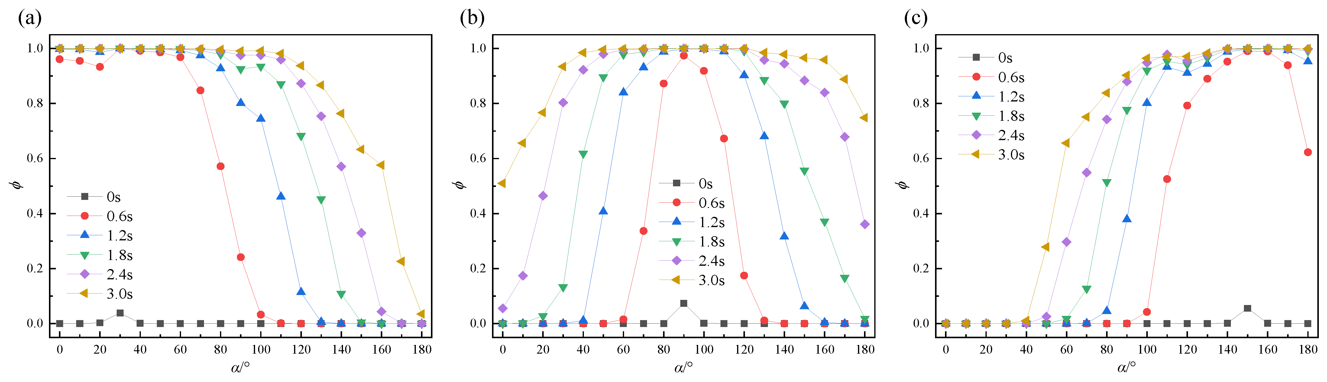
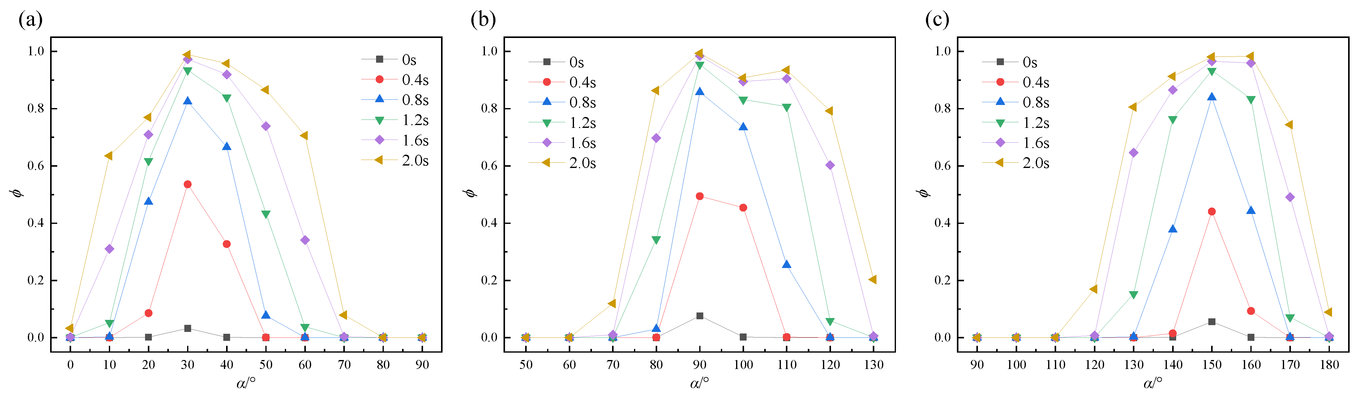
When grout diffuses downward, the diffusion speed is relatively fast, and the transition zone between the grout and air is longer. In contrast, when grout diffuses upward, the diffusion speed is slower, and the transition zone is shorter. Under the same time conditions, the grouting effect is better when the grouting port is at 90° compared to the cases at 30° and 150°.

(2)

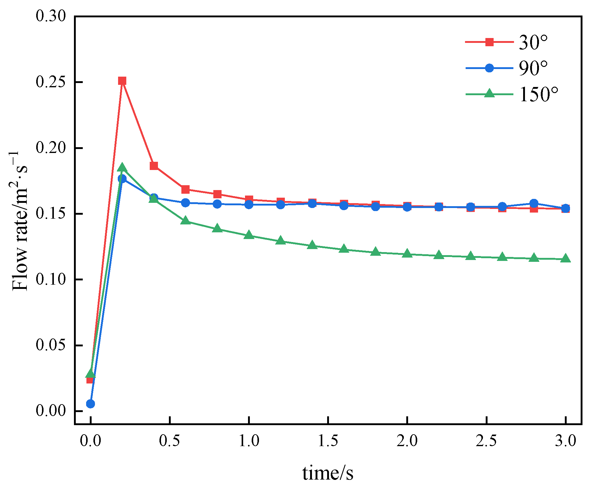
Under the pressure boundar y condition, the grout flow rate increases rapidly during the initial stage and reaches its peak at approximately 0.2 s. The grouting position has a noticeable effect on the peak flow rate: when grouting is applied at the upper part of the segment, the peak flow rate is higher, reaching approximately 0.25 m²/s, whereas grouting at the middle and lower parts results in a lower peak, around 0.18 m²/s. Subsequently, the flow rate gradually decreases and stabilizes, entering a steady-state phase.

(3)

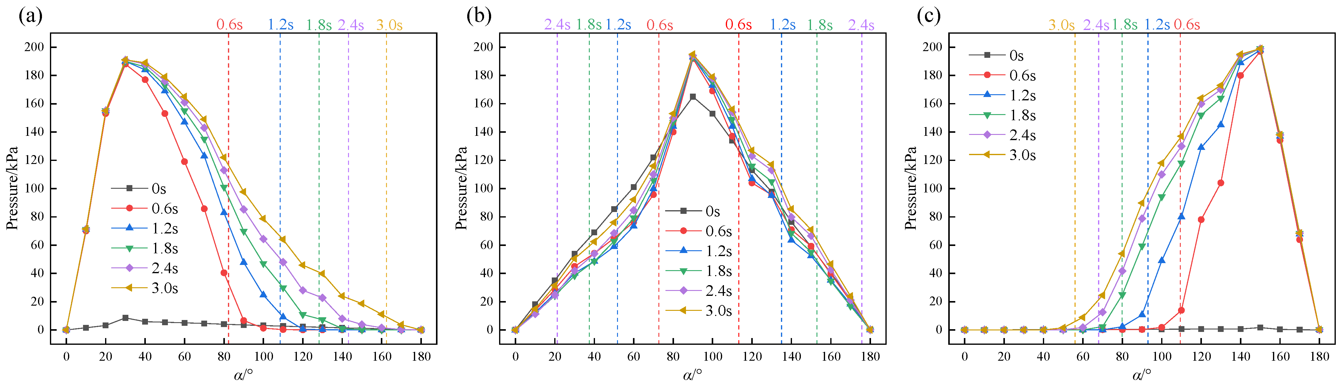
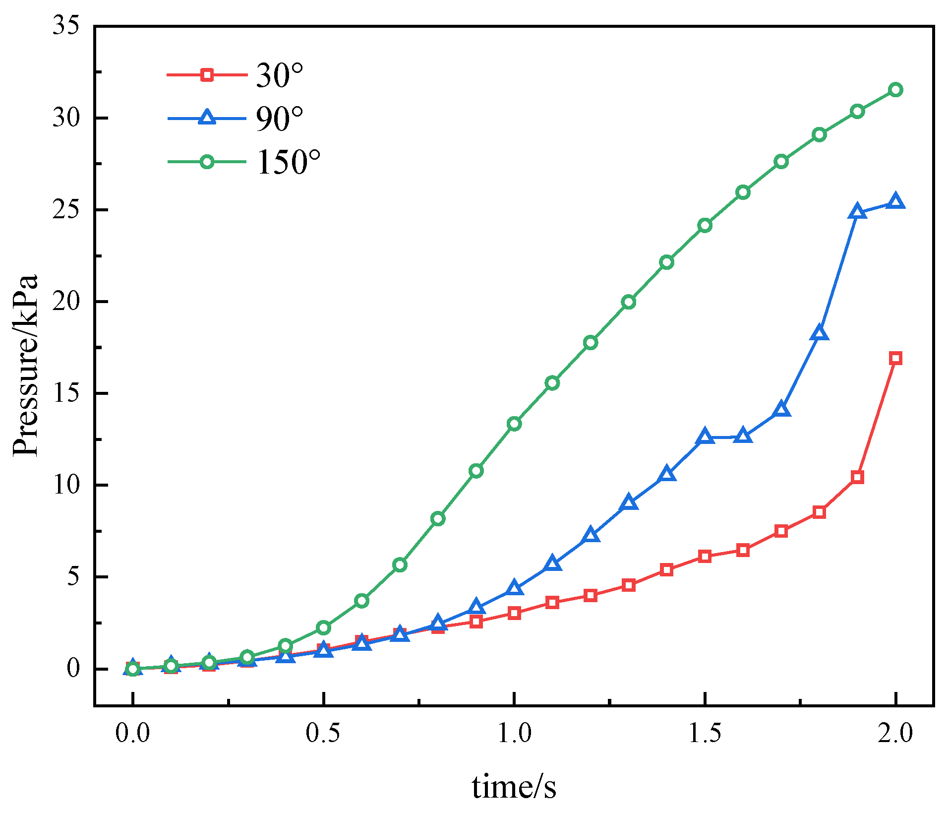
Under velocity boundary conditions, the grouting pressure remains approximately stable during the initial stage of the process. As grouting progresses, the pressure gradually increases. The position of the grouting port has a significant influence on the pressure variation: the lower the port is positioned, the faster the pressure increases. At 2 s into the grouting process, the grouting pressures at the upper, middle, and lower ports are 16.92 kPa, 25.40 kPa, and 31.54 kPa, respectively. The abnormally high grouting pressure may be attributed to locally dense regions, which increase flow resistance and consequently result in elevated grouting pressure.

(4)

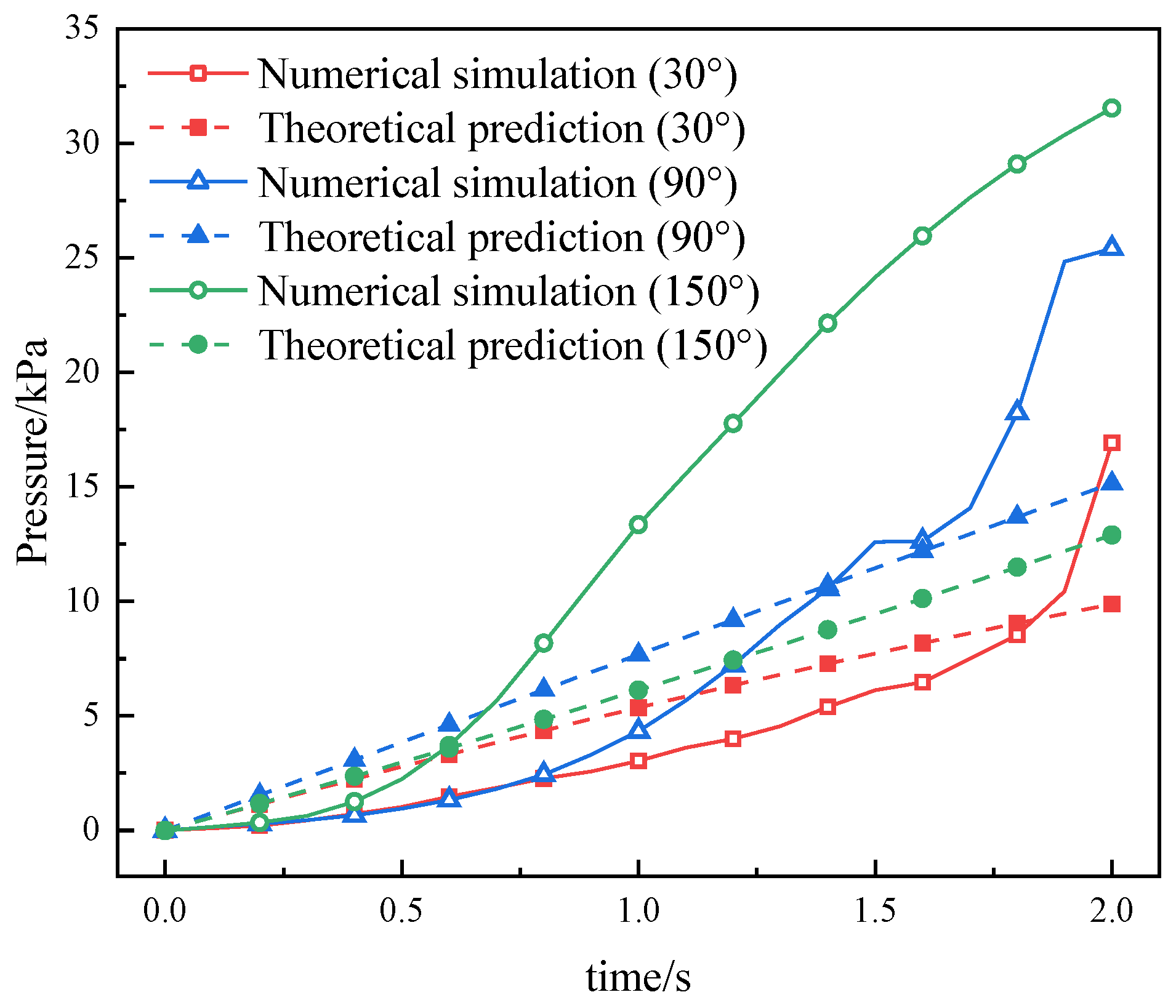
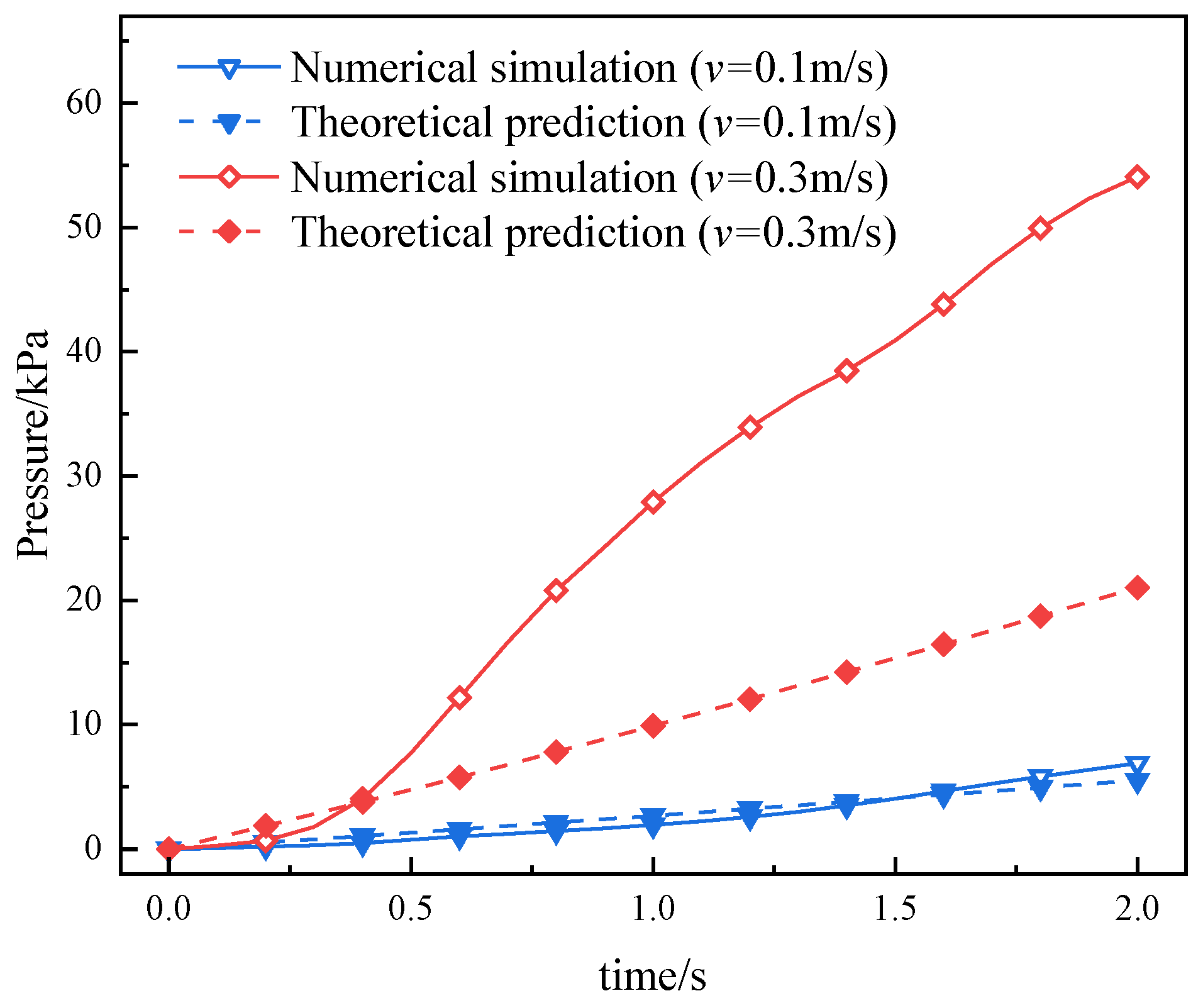
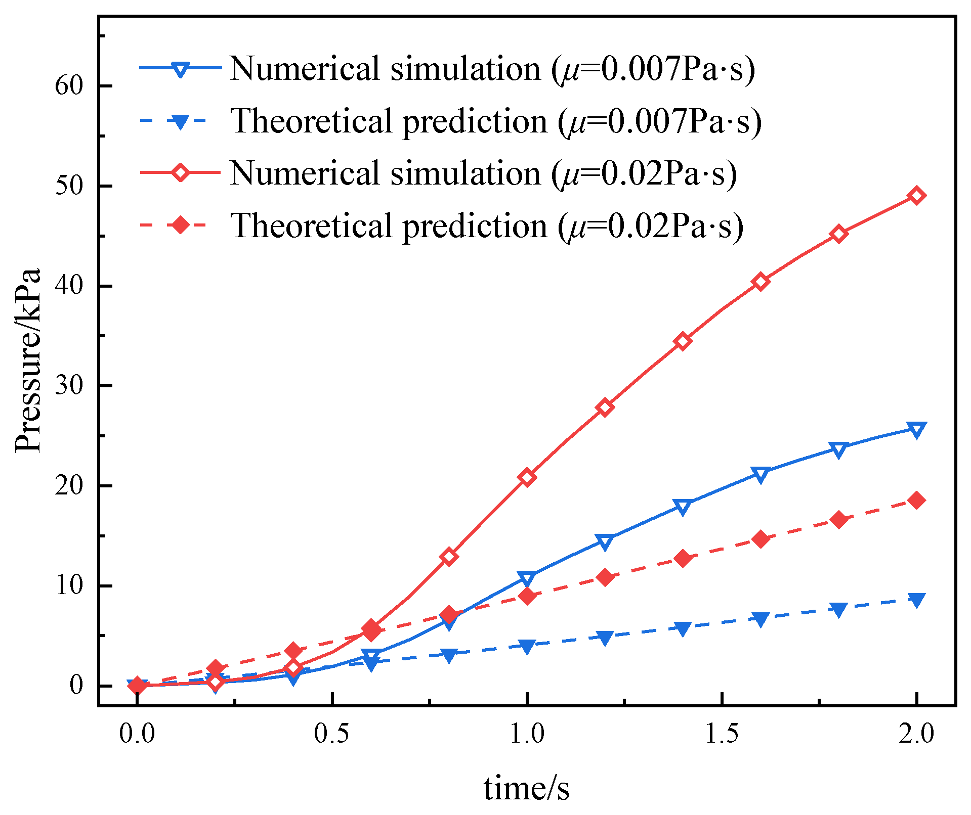
The analytical formula developed in this study can predict the variation in grouting pressure to a certain extent. Compared to the predicted values, the simulated pressures are lower in the early stage of grouting and higher in the later stage. Porosity, grout viscosity, and injection velocity all have significant effects on grouting pressure. As porosity decreases or injection velocity increases, the discrepancy between the numerical simulation results and the theoretical predictions becomes more pronounced, indicating that the existing formula provides greater accuracy and applicability under low injection velocity conditions.

References

1. Liu, J.; Shi, C.; Lei, M.; Wang, Z.; Lin, Y. A study on damage mechanism modelling of shield tunnel under unloading based on damage–plasticity model of concrete. Eng. Fail. Anal. 2021, 123, 105261. [Google Scholar] [CrossRef]
2. Cheng, Z.L.; Kannangara, K.K.P.M.; Su, L.J.; Zhou, W.H. Mathematical model for approximating shield tunneling-induced surface settlement via multi-gene genetic programming. Acta Geotech. 2023, 18, 4923–4940. [Google Scholar] [CrossRef]
3. Wang, Z.; Jiang, Y.; Shao, X.; Liu, C. On-site measurement and environmental impact of vibration caused by construction of double-shield TBM tunnel in urban subway. Sci. Rep. 2023, 13, 17689. [Google Scholar] [CrossRef]
4. Hou, S.; Liu, Y.; Zhuang, W.; Zhang, K.; Zhang, R.; Yang, Q. Prediction of shield jamming risk for double-shield TBM tunnels based on numerical samples and random forest classifier. Acta Geotech. 2023, 18, 495–517. [Google Scholar] [CrossRef]
5. Xu, X.; Wu, Z.; Weng, L.; Chu, Z.; Liu, Q.; Zhou, Y. Numerical investigation of geostress influence on the grouting reinforcement effectiveness of tunnel surrounding rock mass in fault fracture zones. J. Rock Mech. Geotech. Eng. 2024, 16, 81–101. [Google Scholar] [CrossRef]
6. Gan, X.; Yu, J.; Gong, X.; Hou, Y.; Zhu, M. Response of operating metro tunnels to compensation grouting of an underlying large-diameter shield tunnel: A case study in Hangzhou. Undergr. Space 2021, 7, 219–232. [Google Scholar] [CrossRef]
7. Ma, F. Recent Advances in the GPR Detection of Grouting Defects behind Shield Tunnel Segments. Remote Sens. 2021, 13, 4596. [Google Scholar] [CrossRef]
8. Sun, X.; Wang, Y.; Liu, H.; Yang, Z.; Ma, H. Development of multivariate-coupled grouting diffusion model for RCC. Constr. Build. Mater. 2024, 435, 136748. [Google Scholar] [CrossRef]
9. Wang, H.; Yu, Y.; Zhang, P.; Yang, C.; Wen, H.; Zhang, F.; Du, S. Study on the Diffusion Mechanism of Infiltration Grouting in Fault Fracture Zone Considering the Time-Varying Characteristics of Slurry Viscosity Under Seawater Environment. Int. J. Concr. Struct. Mater. 2024, 18, 65. [Google Scholar] [CrossRef]
10. Vorschulze, F.C. Variations in the rheology and penetrability of cement-based grouts—An experimental study. Cem. Concr. Res. 2004, 34, 1111–1119. [Google Scholar] [CrossRef]
11. Jiang, D.; Cheng, X.; Luan, H.; Wang, T.; Zhang, M.; Hao, R. Experimental Investigation on the Law of Grout Diffusion in Fractured Porous Rock Mass and Its Application. Processes 2018, 6, 191. [Google Scholar] [CrossRef]
12. Huayang, L.; Wangwei, Q.; Qianqian, L.; Caifeng, H. Study on the Impact of the Grouting Factors on Surface Subsidence in the Process of Shield Construction. Chin. J. Undergr. Space Eng. 2015, 11, 1303–1309. [Google Scholar]
13. Yanbin, F.U.; Jun, Z.; Xiang, W.U.; Jingyu, Z. Back-fill Pressure Model Research of Simultaneous Grouting for Shield Tunnel. J. Disaster Prev. Mitig. Eng. 2016, 36, 107–113. [Google Scholar]
14. Mittag, J.; Salvidis, S.A. The groutability of sands—Results from one-dimensional and spherical tests. In Grouting and Ground Treatment; ASCE Library: Lawrence, MA, USA, 2003. [Google Scholar] [CrossRef]
15. Maghous, S.; Saada, Z.; Dormieux, L.; Canou, J.; Dupla, J.C. A model for in situ grouting with account for particle filtration. Comput. Geotech. 2007, 34, 164–174. [Google Scholar] [CrossRef]
16. Eklund, D.; Stille, H. Penetrability due to filtration tendency of cement-based grouts. Tunn. Undergr. Space Technol. 2008, 23, 389–398. [Google Scholar] [CrossRef]
17. Axelsson, M.; Gustafson, G.; Fransson, A. Stop mechanism for cementitious grouts at different water-to-cement ratios. Tunn. Undergr. Space Technol. 2009, 24, 390–397. [Google Scholar] [CrossRef]
18. Lee, M.S.; Kim, J.S.; Lee, S.D.; Choi, Y.J.; Lee, I.M. Effect of Vibratory Injection on Grout Permeation Characteristics. Prog. Theor. Phys. 2010, 26, 73–84. [Google Scholar]
19. Weng, L.; Wu, Z.; Zhang, S.; Liu, Q.; Chu, Z. Real-time characterization of the grouting diffusion process in fractured sandstone based on the low-field nuclear magnetic resonance technique. Int. J. Rock Mech. Min. Sci. 2022, 152, 105060. [Google Scholar] [CrossRef]
20. Wang, C.; Diao, Y.; Guo, C.; Li, P.; Du, X.; Pan, Y. Two-stage column–hemispherical penetration diffusion model considering porosity tortuosity and time-dependent viscosity behavior. Acta Geotech. 2022, 18, 2661–2680. [Google Scholar] [CrossRef]
21. Gou, C.F.; Ye, F.; Zhang, J.L.; Liu, Y.P. Ring distribution model of filling pressure for shield tunnels under synchronous grouting. Chin. J. Geotech. Eng. 2013, 35, 590–598. [Google Scholar]
22. Ye, F.; Yang, T.; Mao, J.H.; Qin, X.Z.; Zhao, R.L. Half-spherical surface diffusion model of shield tunnel back-fill grouting based on infiltration effect. Tunn. Undergr. Space Technol. 2019, 83, 274–281. [Google Scholar] [CrossRef]
23. Liu, J.; Li, P.; Shi, L.; Fan, J.; Huang, D. Spatial distribution model of the filling and diffusion pressure of synchronous grouting in a quasi-rectangular shield and its experimental verification. Undergr. Space 2021, 6, 650–664. [Google Scholar] [CrossRef]
24. Ma, J.; Sun, A.; Jiang, A.; Guo, N.; Liu, X.; Song, J.; Liu, T. Pressure Model Study on Synchronous Grouting in Shield Tunnels Considering the Temporal Variation in Grout Viscosity. Appl. Sci. 2023, 13, 10437. [Google Scholar] [CrossRef]
25. Rosquot, F.; Alexis, A.; Khelidj, A.; Phelipot, A. Experimental study of cement grout: Rheological behavior and sedimentation. Cem. Concr. Res. 2003, 33, 713–722. [Google Scholar] [CrossRef]
26. Zhou, M.; Fan, F.; Zheng, Z.; Ma, C. Modeling of Grouting Penetration in Porous Medium with Influence of Grain Distribution and Grout–Water Interaction. Processes 2021, 10, 77. [Google Scholar] [CrossRef]
27. Gustafson, G.; Claesson, J.; Fransson, S. Steering Parameters for Rock Grouting. J. Appl. Math. 2013, 1, 269594. [Google Scholar] [CrossRef]
28. Zhu, G.; Zhang, Q.; Liu, R.; Bai, J.; Li, W.; Feng, X. Experimental and numerical study on the permeation grouting diffusion mechanism considering filtration effects. Geofluids 2021, 1, 6613990. [Google Scholar] [CrossRef]
29. Zhang, Q.S.; Wang, H.B.; Liu, R.T.; Li, S.C.; Zhang, L.W.; Zhu, G.X.; Zhang, L.Z. Infiltration grouting mechanism of porous media considering diffusion paths of grout. Chin. J. Geotech. Eng. 2018, 40, 918–924. [Google Scholar] [CrossRef]
Figure 1. Research roadmap.
Applsci 15 07542 g001
Figure 2. Backfilling layer and pea gravel: (a) backfilling layer; (b) pea gravel.
Applsci 15 07542 g002
Figure 3. Simulation of pea gravel consolidation.
Applsci 15 07542 g003
Figure 4. Generation process of the porous media model.
Applsci 15 07542 g004
Figure 5. Geometric model and boundary conditions: (a) geometric model; (b) boundary conditions; (c) isolated zone.
Applsci 15 07542 g005
Figure 6. Grout diffusion (α = 90°).
Applsci 15 07542 g006
Figure 7. Grout diffusion: (a) α = 30°; (b) α = 150°.
Applsci 15 07542 g007
Figure 8. Local analysis of pressure and velocity field of grout in the backfilling layer: (a) pressure contour; (b) velocity contour; (c) streamline plot.
Applsci 15 07542 g008
Figure 9. Grout filling condition in the backfilling layer under pressure boundary conditions. (a) α = 30°; (b) α = 90°; (c) α = 150°.
Applsci 15 07542 g009
Figure 10. Grout pressure distribution in the backfilling layer under pressure boundary conditions. (a) α = 30°; (b) α = 90°; (c) α = 150°.
Applsci 15 07542 g010
Figure 11. Flow rate variation at grouting port.
Applsci 15 07542 g011
Figure 12. Grout filling condition in the backfilling layer under velocity boundary conditions. (a) α = 30°; (b) α = 90°; (c) α = 150°.
Applsci 15 07542 g012
Figure 13. Grout pressure distribution in the backfilling layer under velocity boundary conditions. (a) α = 30°; (b) α = 90°; (c) α = 150°.
Applsci 15 07542 g013
Figure 14. Variation in grouting pressure.
Applsci 15 07542 g014
Figure 15. Force analysis of fluid microelement.
Applsci 15 07542 g015
Figure 16. Analysis of grout diffusion.
Applsci 15 07542 g016
Figure 17. Simulated grouting pressure versus values predicted by formula.
Applsci 15 07542 g017
Figure 18. Effect of porosity variation on grouting pressure.
Applsci 15 07542 g018
Figure 19. Effect of injection velocity on grouting pressure.
Applsci 15 07542 g019
Figure 20. Effect of grout viscosity on grouting pressure.
Applsci 15 07542 g020
Figure 21. Laboratory grouting pressure measurements with fixed injection rates.
Applsci 15 07542 g021