Article

G-CTRNN: A Trainable Low-Power Continuous-Time Neural Network for Human Activity Recognition in Healthcare Applications

1
Durham School of Architectural Engineering & Construction, College of Engineering, University of Nebraska-Lincoln, Omaha, NE 68182, USA
2
GE Aerospace Research, Niskayuna, NY 12309, USA
*
Author to whom correspondence should be addressed.
Appl. Sci. 2025, 15(13), 7508; https://doi.org/10.3390/app15137508
Submission received: 29 May 2025 / Revised: 21 June 2025 / Accepted: 23 June 2025 / Published: 4 July 2025
(This article belongs to the Special Issue Human Activity Recognition (HAR) in Healthcare, 3rd Edition)

Abstract

Featured Application

Real-time, on-device human activity recognition using low-power MEMS-based wearables for remote patient monitoring, fall detection and personalized healthcare in resource-constrained edge environments.

Abstract

Continuous-time Recurrent Neural Networks (CTRNNs) are well-suited for modeling temporal dynamics in low-power neuromorphic and analog computing systems, making them promising candidates for edge-based human activity recognition (HAR) in healthcare. However, training CTRNNs remains challenging due to their continuous-time nature and the need to respect physical hardware constraints. In this work, we propose G-CTRNN, a novel gradient-based training framework for analog-friendly CTRNNs designed for embedded healthcare applications. Our method extends Backpropagation Through Time (BPTT) to continuous domains using TensorFlow’s automatic differentiation, while enforcing constraints on time constants and synaptic weights to ensure hardware compatibility. We validate G-CTRNN on the WISDM human activity dataset, which simulates realistic wearable sensor data for healthcare monitoring. Compared to conventional RNNs, G-CTRNN achieves superior classification accuracy with fewer parameters and greater stability—enabling continuous, real-time HAR on low-power platforms such as MEMS computing networks. The proposed framework provides a pathway toward on-device AI for remote patient monitoring, elderly care, and personalized healthcare in resource-constrained environments.

1. Introduction and Literature Review

1.1. Introduction

Human Activity Recognition (HAR) has become a cornerstone technology in modern healthcare systems, enabling applications such as fall detection, chronic disease monitoring, rehabilitation tracking, and ambient assisted living [1,2]. With the increasing adoption of wearable sensors and edge AI, there is a growing need for machine learning models that can operate in real time and under strict energy and hardware constraints. In this context, Continuous-Time Recurrent Neural Networks (CTRNNs) offer an analog-friendly, biologically inspired framework for modeling temporal dynamics in continuous data streams [3,4], such as acceleration signals from wearable healthcare devices. Their formulation using differential equations allows direct mapping onto low-power embedded hardware like mixed-signal processors [5] and MEMS sensors [6,7,8]. However, a persistent barrier to their practical adoption is the difficulty of training such systems using gradient-based methods, especially when time constants and other physical parameters must remain bounded and interpretable [9].
Traditional training techniques for recurrent networks, such as Backpropagation Through Time (BPTT), are typically applied in discrete time and do not directly extend to physical systems governed by continuous dynamics. Moreover, existing approaches often fail to account for hardware constraints, including energy efficiency, device variability, and limited tunability of analog parameters. In this paper, we introduce G-CTRNN, a gradient-based training framework for analog-friendly CTRNNs, tailored specifically for low-power healthcare-focused HAR applications. Implemented in TensorFlow, our approach extends BPTT to continuous-time networks while enforcing parameter constraints that reflect real-world hardware requirements. This makes it uniquely suited for real-time HAR on low-power embedded systems such as MEMS sensors used in wearables. We validate G-CTRNN using the WISDM dataset, which contains smartphone-based activity data commonly used in healthcare applications. The results show that G-CTRNN provides superior accuracy and efficiency compared to traditional RNNs while significantly reducing the number of parameters and resource consumption.

1.2. Related Work

CTRNNs were initially introduced as continuous analogs to traditional RNNs, capable of modeling the temporal evolution of dynamical systems [2,3,4]. Funahashi and Nakamura [9] demonstrated that CTRNNs can approximate any dynamical system given enough neurons, laying a theoretical foundation for their use in temporal learning tasks. Beer [3] later extended these ideas by applying CTRNNs to biologically inspired agents in evolutionary robotics, highlighting their capacity to capture complex temporal behaviors.
Despite their potential, training CTRNNs remains a bottleneck. Traditional methods like genetic algorithms [10] and differential evolution [11] have been explored, particularly in low-data or hardware-constrained scenarios. While these approaches provide flexibility in parameter search, they suffer from scalability issues and slow convergence. More recently, advances in neural ordinary differential equations (Neural ODEs) have enabled differentiable modeling of continuous-time systems [12]. These models integrate deep learning with ODE solvers and backpropagation through continuous-time dynamics. Our approach builds on these ideas by incorporating automatic differentiation and constrained optimization of time constants within a CTRNN framework, aligning with recent efforts to make continuous-time models trainable and scalable [13].
Recent research has also explored advanced strategies for improving learning efficiency and human activity recognition. Orthogonal learning designs have been applied to enhance the performance of metaheuristic optimization algorithms [14], while fuzzy architecture search with classifier-assisted multi-objective optimization shows promise in tuning neural models [15]. In the context of HAR, attention-based temporal convolutional networks have improved sequential modeling performance [16], and cross-modal federated learning has enabled privacy-preserving activity recognition across devices [17]. These efforts highlight the ongoing push toward efficient, robust, and scalable AI models, which align with the goals of G-CTRNN for edge deployment in healthcare.

2. Continuous-Time Recurrent Neural Network (CTRNN)

This section aims to describe the continuous-time recurrent neural network mathematical model and its analogy to physical systems such as MEMS computing networks.

2.1. CTRNN Model

The CTRNN mathematical model consists of six preliminary components, as shown in Figure 1a and Equation (1). The differential part in Equation (1) makes them intricately intertwined to mimic the behavior of human brain neuron cells [12]:
τ i d y i d t = y i + f i ( B i + j = 1 n w i j . y j ) + I i ( t )
where τ i is the time constant of neuron i; y i i and f i i are the state and activation function of the ith neuron; and w i j , B i , I i ( t ) represent the weight vector, bias shift, and external input at time t of the ith neuron. The first part of the neuron is the continuous state of the current neuron, represented by y i This state changes over time and depends on the previous state and all the other five components. The second part is the activation or nonlinearity function, which is denoted as f i , the Sigmoid function. Rectified Linear Units (ReLUs) and hyperbolic tangent functions (Tanhs) are all examples of widely used non-linear functions. The behavior of a biological neuron inspires the activation function to capture the nonlinearity of a complex pattern. As a group of neurons activate together, signal propagation occurs through them in a specific path. Different paths capture different patterns. The third part is the synaptic weight vector, represented as w i j . It describes the strength of the connection between neurons j and i. The fourth part is the external input, I i ( t ) , representing the continuous input signal from the sensors or other data sources. The fifth part is the time constant represented by τ i , which controls how quickly the current cell reacts to any external input; a high τ means the neuron needs more time to respond and change its status, while a low time constant means this neuron has a rapid response to any change. The last part is the neuron dynamics, represented by the state’s rate of change (differential part), represented by d y i d t .

2.2. MEMS Analogy

As stated before and shown in Figure 1b, the MEMS dynamics can be engineered to match the equation of a continuous-time recurrent neuron [6,7,8]. Thus, eventually, the MEMS can perform the CTRNN calculation without the need for a computer. In this mapping, the time constant τ in the CTRNN corresponds to the mechanical time constant of MEMS resonators, governed by the mass-to-damping coefficient ratio. Synaptic weights can be mapped to coupling stiffness values or transconductance gains in MEMS electro-mechanical systems, while biases relate to baseline actuation voltages or equilibrium positions. However, practical limitations must be considered. MEMS devices are affected by process variability, temperature-dependent drift, and mechanical noise, which may introduce deviations from ideal continuous-time behavior. Despite these challenges, recent work in analog computing shows promise in mitigating such effects through calibration and robust design strategies.

2.3. Time Constant Effect

To study the effect of the time constant on the CTRNN response, we discretize the CTRNN, as shown in Equation (2), using the Euler method.
y i + 1 = [ y i + 1 τ i [ y i + f i ( B i + j = 1 n w i j . y j ) ] + I i ( t ) ]
where h is the Euler democratization step size; τi is the time constant for the ith neuron. Equation (2) implies that when τi approaches a large value, the subsequent state yi+1 equals the current state yi (tiny change). Conversely, when τi approaches zero, the next state will be strongly influenced by input changes or the status of other neurons. It is crucial to select the τ value greater than h, as if h >> τ, Equation (2) indicates that the second term of the equation will be multiplied by a value greater than 1, causing system instability. This instability arises from amplifying the other neurons’ external input and output, leading to an unstable neuron state. Equation (2) recommends choosing h << τ to ensure the neurons and the model’s stability.

3. Model Development and Training

In this section, we discuss the human activity training data and the development of the G-CTRNN model to classify them. We also explain the training algorithms to learn and optimize the model parameters.

3.1. Human Activity Detection

We used human activity detection applications to verify our G-CTRNN model and to ensure its real-world applicability, test its temporal learning capabilities, validate its performance, and facilitate comparative analysis with other models in activity recognition tasks. Human activity detection has many field applications, including healthcare, security, robotics, and smart buildings [18,19]. Many technologies were utilized to implement human activity detection, like wearable, camera-based, infrared (IR), and Wi-Fi sensors [20]. Human activity detection enables intelligent, responsive environments that adapt to the residents’ needs and preferences. Recognizing human activities will also help save energy consumption, enhance security, improve indoor environmental quality, and provide personalized services. For example, ref. [21] employed human activity recognition to manage HVAC systems, lighting, heating, ventilation, and air conditioning by responding to occupancy and activity patterns, decreasing energy usage, and enhancing energy efficiency. Moreover, the work in [22] utilized human activity recognition, which identifies irregularities, like unauthorized access or atypical behavior, thereby bolstering security measures and thwarting potential intrusions.
In this work, we used the WISDM (Wireless Sensor Data Mining) dataset for training and testing G-CTRNN. The WISDM data contains six attributes extracted from smartphones for various groups of people while carrying those devices. The data contains six activities: jogging, walking, upstairs–downstairs, sitting, and standing, as shown in Figure 2. The data holds significant prominence in the literature due to its widespread utilization and well-organized structure [23]. However, while the WISDM dataset demonstrates the feasibility of applying G-CTRNN to sensor-based human activity recognition, we acknowledge its limitations in representing clinical scenarios. The dataset involves healthy subjects performing standard activities, which may not capture the complexity of gait abnormalities, post-surgical recovery movements, or neurological impairments. Future work will include validating G-CTRNN on more diverse and clinically representative datasets to assess its broader applicability in healthcare contexts.

3.2. Model Structure

As shown in Figure 3, the model consists of a set of consecutive connected layers. The first layer has sixteen recurrent cells. The first layer is fully connected to the second layer, which has ten cells. The final layer has six cells, one for each human activity. The model systematically traverses the dataset. We used well-known algorithms called sliding windows [24]. The algorithm employs a predetermined window size and constant sliding steps. The purpose is to group subsequent records into one entity. Based on the literature, we picked the window size to be fifty records, corresponding to approximately 2.5 s at WISDM’s 20 Hz sampling rate. While this fixed-window method is standard for WISDM, we acknowledge that different healthcare applications may require varying temporal resolutions from sub-second seizure detection to multi-minute rehabilitation tracking. Future work may consider adaptive windowing strategies to dynamically adjust window lengths based on signal characteristics or medical context.
To maintain data integrity, we only include instances where the dominating activity constitutes at least 70% of the observations in the training phase. Including this percentage will ensure a higher degree of activity purity. The data was divided into three distinct portions. Precisely 10% was allocated for testing, and 90% was left for training. From the training data, 10% was reserved as a validation dataset to evaluate the model’s performance while training, which will help the model avoid problems like overfitting, a scenario where the model performs well during training but poorly when applied to testing data.

3.3. Backpropagation and Backpropagation Through Time

The universal approximation theorem states that a neural network with sufficient neurons and appropriate activation functions can approximate any continuous function [25]. The neural network is a set of interconnected layers containing a vector of neurons. The vision of machine learning is to approximate desired functions by learning the best weights that map the input to the output. The main challenge is training the model and updating the weights to optimize the model’s mathematical function. The most popular technique for training is backpropagation. Typically, when data is fed into the neural network, it flows sequentially from the input layer to the hidden layer and finally to the output layer. The output is then compared to the ground truth (the true data). The loss is a function that mirrors the difference between our model expectation and the true data and is computed.
The backpropagation adjusts the weight of the whole network starting from the output layer and propagates back into the input layer to reduce the loss function (reduce the error). As the training goes back through each layer and reaches the recurrent layer with a self-loop, the recurrent layer should be unfolded [26]. Thus, the backpropagation method must go through every step to train the inner weights. To achieve this, the G-CTRNN uses the Backpropagation Through Time (BPTT) concept to adjust the internal weights and the time constant. In the continuous-time domain, BPTT unfolds the recurrent neural network over time by discretizing it into small time steps and computing gradients through each time step to update weights using the chain rule. We chose BPTT because it is the standard approach for training continuous-time recurrent models where hidden states depend on past temporal dynamics, which is central to G-CTRNN operation.
To train the G-CTRNN using the BPTT, it is necessary to solve the associated ordinary differential equations (ODEs). One commonly used numerical method for solving ODEs is the Euler method [27], derived from the Taylor series. The G-CTRNN Euler representation was implemented using the TensorFlow library 2.8. TensorFlow is esteemed for its modern design, reliability, and adaptability [28]. In this implementation, the TensorFlow engine converts the network to a static computation graph before training, allowing full GPU acceleration and parallelism compatibility [29]. Figure 4 shows the steps to implement the forward and backward passes in TensorFlow for the G-CTRNN. These passes are tightly coupled in TensorFlow, but we separated them in the figure to illustrate the implementation details more clearly. In these steps, the auto-differentiation engine in TensorFlow traces the computational graph over all unrolled time steps. Using the chain rule, gradients are computed for both synaptic weights and time constants. The built-in ADAM optimizer updates parameters, with modifications to accommodate time-constant tuning. The ADAM Optimizer employs adaptive learning rates to accelerate the convergence of the model. During the initial learning phase of the model, it commences with a random initialization [30]. The ADAM optimizer leverages a movement’s momentum to accelerate the progression consistently, leading to smooth convergences.

3.4. G-CTRNN Time Constant Training

Training the time constant in the G-CTRNN using the BPTT is challenging, as this parameter has a physical meaning and some restrictions, such as that it should be a positive number within a specific range. The regularization technique is one option to solve this problem by limiting the training time constant to account for this constraint. In this method, the parameter of interest, the time constant here, will be added to the loss function to force the training to minimize those parameters [31]. However, this method will not guarantee that the parameter (time constant) does not exceed a specific value. Alternatively, TensorFlow has a non-popular functionality to override the constraints of the parameters of each cell to have values from a specific distribution [32]. In this work, we adapted this method to limit the time constant value during the training. This constraint will use the MINMAX Norm, which will constrain the values of the weights of any layers to have the norm between a lower bound and an upper bound.
Finally, it is worth mentioning that our implementation adopts a single time constant per neuron to maintain architectural simplicity and facilitate hardware integration. While this approach effectively stabilizes training and ensures feasibility under physical constraints, modeling temporal complexity in some applications, such as healthcare, may benefit from extended architectures. Specifically, incorporating multiple time constants per neuron or introducing hierarchical time scales would allow simultaneous encoding of rapid signals (e.g., tremors) and slower trends (e.g., postural transitions). These architectural variations present a promising direction for future research to generalize G-CTRNN across multi-scale scenarios.

4. Result

4.1. Time-Constant Effects

This section presents the results of using the G-CTRNN for human activity classification. We built the G-CTRNN and compared it to the standard RNN. We also examine the importance of training the time constant parameter and its significant impact on the accuracy of the G-CTRN model. Toward this objective, we conducted different experiments. The initial investigation involved training the model by setting a time constant value equal to a constant value of one in all sixteen cells of the first layer, which is the standard practice in the literature. The time constant values were next initialized in the subsequent experiment using a uniform random distribution with a range of [0, 2]. Finally, for the first time, the time constant of each cell in G-CTRNN is trained using backpropagation through time. The models were trained for 50 epochs in all scenarios, and the G-CTRNN results were compared to the standard RNN.
The RNN model shows poor performance with inconsistent accuracy as the number of epochs increases despite all the models using the same optimizer and starting with the same learning rate. The G-CTRNN model with the time constant set to one shows an accuracy of 68%, and the model successfully converged smoothly throughout 50 epochs. The G-CTRNN model had a better learning opportunity when the time constant was randomly initialized (resulting in varying time constant values for each cell). This is because different time constant values imply different response speeds for each cell, essential for extracting knowledge from the sequence data. The accuracy in this scenario improved to 76%, as depicted in Figure 5. Finally, an accuracy of 81.9% was achieved when the G-CTRNN time constants were included in the training. In summary, Figure 5 shows that G-CTRNN exhibits smoother convergence and improved stability across epochs compared to traditional RNNs, which suffer from inconsistent learning and catastrophic forgetting. The ability to adjust time constants dynamically contributes to G-CTRNN’s robust and efficient convergence behavior. Finally, Table 1 summarizes our findings concerning the different time-constant scenarios. All models started with the same learning rate to ensure a fair comparison: 0.001, the default value for ADAM algorithms in Keras 2.8.
In addition to the time-constant variations, we conducted internal ablation studies to validate key design choices. Removing the MINMAX constraint on the time constant resulted in numerical instability and occasional divergence during training, confirming the necessity of enforcing physical bounds. Similarly, using standard discrete-time backpropagation instead of continuous-time BPTT led to significant performance degradation and failure to converge when training the time constant, underscoring the importance of using continuous-time gradient propagation for temporal consistency and parameter sensitivity.
Finally, it is worth noting that while our experimental comparison centers on traditional RNNs due to their structural similarity to the G-CTRNN, we note that other lightweight models such as Gated Recurrent Units (GRUs), Echo State Networks (ESNs), and Spiking Neural Networks (SNNs) have also been proposed for efficient temporal modeling. GRUs simplify gating mechanisms to reduce parameter count, ESNs offload learning to the readout layer but require careful reservoir tuning, and SNNs operate with biologically inspired spike timing but often demand event-based hardware. In contrast, G-CTRNN offers a compact continuous-time formulation amenable to analog or MEMS-based hardware, providing a balance between trainability and low-power implementation. Future work will expand experimental comparisons to include these models.
Full evaluation metrics, including confusion matrices, sensitivity, and specificity for each classified activity across all models, are provided in Appendix A for further reference.

4.2. A Parameter Size Comparison Between RNN and G-CTRNN

The G-CTRNN model is a sequence of layers. Each layer is a set of cells, and each cell has different parameters that control the behavior of those cells. This section compares the different G-CTRNN and RNN models regarding parameter count and accuracy (Table 2). G-CTRNN reached an accuracy of about 82% with a total number of 572 parameters. The RNN reaches 73%, using almost the same number of parameters. To reach an accuracy close to the RNN accuracy, the G-CTRNN has only four neurons in the first layer. In this case, the G-CTRNN parameters are only 152, about 27% of the RNN parameters (less than one-third of the parameters!). The subsequent inquiry in the investigation pertains to determining the requisite number of parameters for the RNN to achieve an accuracy of 81.9%. RNN, with a parameter count of 1,548, achieved an accuracy of 81.4%, which falls short of the performance exhibited by the G-CTRNN with only 572 parameters. Therefore, the G-CTRNN, while having just 38% of the parameters, showed superior performance compared to the RNN.

4.3. Computational Overhead

Including continuous-time dynamics in G-CTRNN adds considerable computational load during training. Solving differential equations with Euler integration, combined with gradient-based optimization of the time constant under parameter constraints, lengthens the per-epoch training time. In our experiments, training G-CTRNN for 50 epochs on a machine equipped with an Intel Xeon CPU and 16 GB RAM took about 6.5 h, while a comparable RNN was trained in under 1 h (approximately 56 min) on the same setup. This reflects a 7× increase in training time due to the overhead of resolving continuous dynamics and enforcing parameter constraints. However, during inference, the target physical implementations—such as a MEMS-based or analog hardware system—will naturally solve the differential equations in real time through their intrinsic dynamics. Consequently, the computational burden at deployment shifts from software-based simulation to native physical processes, allowing for energy-efficient, real-time operation on edge devices.

5. Conclusions

In this paper, we introduced G-CTRNN, a novel gradient-based training framework for Continuous-Time Recurrent Neural Networks (CTRNNs), designed to enable efficient learning on hardware-constrained platforms such as MEMS-based or analog signal processors. Unlike conventional RNNs or heuristic-based CTRNNs, G-CTRNN leverages differentiable programming and constraint-aware optimization to train both synaptic weights and neuron time constants in a biologically inspired, real-time-compatible fashion.
We evaluated G-CTRNN on the WISDM dataset, a widely used benchmark for human activity recognition (HAR) from wearable sensor data. The results demonstrate that G-CTRNN outperforms traditional RNNs in terms of accuracy, convergence stability, and parameter efficiency—qualities that are particularly important for healthcare applications such as elderly monitoring, activity-based diagnosis, and remote rehabilitation support. G-CTRNN also shows strong promise for low-power operation, making it well-suited for edge deployment in wearable or mobile health systems.
These results suggest that G-CTRNN is a promising model for real-time embedded AI, assuming physical implementations (e.g., MEMS or analog hardware) that can passively solve the differential dynamics without iterative digital computation. While the current simulation uses Euler integration, which incurs computational overhead, such constraints must be mitigated in native hardware where time dynamics unfold naturally.
Future work will focus on hardware-software co-design for analog and MEMS implementation of G-CTRNN, robustness to sensor noise, and clinical validation in healthcare environments. Overall, this work contributes a significant step toward enabling real-time embedded AI in next-generation healthcare monitoring systems through the integration of machine learning, edge computing, and analog signal processing. Finally, while this work constrains model parameters to remain hardware-compatible, future research will incorporate direct optimization for energy consumption, fabrication variability, and real-world MEMS dynamics during training, enabling even tighter integration between model behavior and physical implementation.

Author Contributions

Methodology, J.R.; formal analysis, A.A.; investigation, A.A.; resources, D.L. and F.A.; writing—review and editing, F.A.; project administration, F.A.; funding acquisition, D.L. All authors have read and agreed to the published version of the manuscript.

Funding

This research is based upon work supported in part by the Office of the Director of National Intelligence (ODNI), Intelligence Advanced Research Projects Activity (IARPA), via [2022-21102100011].

Data Availability Statement

Publicly available datasets were analyzed in this study. This data can be found here: https://www.cis.fordham.edu/wisdm/dataset.php.

Acknowledgments

The views and conclusions contained herein are those of the authors and should not be interpreted as necessarily representing the official policies, either expressed or implied, of ODNI, IARPA, or the U.S. Government. The U.S. Government is authorized to reproduce and distribute reprints for governmental purposes notwithstanding any copyright annotation therein.

Conflicts of Interest

Authors David Lin and Johan Reimann were employed by the company GE Aerospace Research. The remaining author declares that the research was conducted in the absence of any commercial or financial relationships that could be construed as a potential conflict of interest.

Appendix A

To evaluate the classification performance of the proposed G-CTRNN architecture compared to standard RNNs, we measured per-class sensitivity and specificity across six activity categories: Downstairs, Jogging, Sitting, Standing, Upstairs, and Walking. Table A1 summarizes these metrics for both models at different recurrent cell sizes (e.g., 4, 16, 32 cells). Sensitivity reflects the model’s ability to correctly detect instances of a given activity, while specificity captures how well it avoids false positives for that class. This comparison allows us to analyze the behavior of each model under varying computational capacities and assess their suitability for resource-constrained environments or real-time deployment.
Table A1. Comparison of sensitivity and specificity for G-CTRNN and RNN models across activities and cell sizes.
Metric/ModelActivity Name
MetricModel (Cells)DownstairsJoggingSittingStandingUpstairsWalking
SensitivityG-CTRNN (16)0.440.960.930.960.640.88
RNN (32)0.440.960.930.960.600.88
G-CTRNN (4)0.170.880.940.970.460.79
RNN (16)0.440.980.870.960.450.66
SpecificityG-CTRNN (16)0.960.970.990.990.910.94
RNN (32)0.950.970.990.990.910.94
G-CTRNN (4)0.970.940.990.980.910.82
RNN (16)0.960.890.990.970.910.92
Figure A1. The confusion matrix for the G-CTRNN model was trained for 50 epochs with 16 recurrent cells and 6 activity classes. The model achieved an overall classification accuracy of 81.9%.
Applsci 15 07508 g0a1
Figure A2. The confusion matrix for the RNN model was trained for 50 epochs with 32 recurrent cells and 6 activity classes. The model achieved an overall classification accuracy of 81.2%.
Applsci 15 07508 g0a2
Figure A3. The confusion matrix for the G-CTRNN model was trained for 50 epochs with 4 recurrent cells and 6 activity classes. The model achieved an overall classification accuracy of 71.8%.
Applsci 15 07508 g0a3
Figure A4. The confusion matrix for the RNN model was trained for 50 epochs with 16 recurrent cells and 6 activity classes. The model achieved an overall classification accuracy of 73.1%.
Applsci 15 07508 g0a4

References

  1. Yu, Y.; Zhou, Z.; Xu, Y.; Chen, C.; Guo, W.; Sheng, X. Toward Hand Gesture Recognition Using a Channel-Wise Cumulative Spike Train Image-Driven Model. Cyborg Bionic Syst. 2025, 6, 0219. [Google Scholar] [CrossRef] [PubMed]
  2. Luo, M.; Yin, M.; Li, J.; Li, Y.; Kobsiriphat, W.; Yu, H.; Xu, T.; Wu, X.; Cao, W. Lateral Walking Gait Recognition and Hip Angle Prediction Using a Dual-Task Learning Framework. Cyborg Bionic Syst. 2025, 6, 0250. [Google Scholar] [CrossRef] [PubMed]
  3. Beer, R.D. On the dynamics of small continuous-time recurrent neural networks. Adapt. Behav. 1995, 3, 469–509. [Google Scholar] [CrossRef]
  4. Elman, J.L. Finding structure in time. Cogn. Sci. 1990, 14, 179–211. [Google Scholar] [CrossRef]
  5. Cauwenberghs, G. An analog VLSI recurrent neural network learning a continuous-time trajectory. IEEE Trans. Neural Netw. 1996, 7, 346–361. [Google Scholar] [CrossRef] [PubMed]
  6. Alsaleem, F.M.; Hasan, M.H.H.; Tesfay, M.K. A MEMS Nonlinear Dynamic Approach for Neural Computing. J. Microelectromech. Syst. 2018, 27, 780–789. [Google Scholar] [CrossRef]
  7. Emad-Ud-Din, M.; Hasan, M.H.; Jafari, R.; Pourkamali, S.; Alsaleem, F. Simulation for a MEMS-Based CTRNN Ultra-Low Power Implementation of Human Activity Recognition. Front. Digit. Health 2021, 3, 731076. [Google Scholar] [CrossRef]
  8. Rafaie, M.; Hasan, M.H.; Alsaleem, F.M. Neuromorphic MEMS Sensor Network. Appl. Phys. Lett. 2019, 114, 163501. [Google Scholar] [CrossRef]
  9. Funahashi, K.; Nakamura, Y. Approximation of Dynamical Systems by Continuous Time Recurrent Neural Networks. Neural Netw. 1993, 6, 801–806. [Google Scholar] [CrossRef]
  10. De Falco, I.; Tarantino, E.; Della Cioppa, A.; Marcelli, A.; Salvatore, C. CTRNN Parameter Learning Using Differential Evolution. In ECAI 2008; IOS Press: Amsterdam, The Netherlands, 2008; pp. 783–784. [Google Scholar]
  11. Bown, O.; Lexer, S. Continuous-Time Recurrent Neural Networks for Generative and Interactive Musical Performance. In Applications of Evolutionary Computation; Springer: Berlin/Heidelberg, Germany, 2006; pp. 652–663. [Google Scholar]
  12. Chen, R.T.Q.; Rubanova, Y.; Bettencourt, J.; Duvenaud, D. Neural Ordinary Differential Equations. In Proceedings of the 32nd Conference on Neural Information Processing Systems (NeurIPS), Montreal, QC, Canada, 3–8 December 2018; Available online: https://arxiv.org/abs/1806.07366 (accessed on 28 May 2025).
  13. Baydin, A.G.; Pearlmutter, B.A.; Radul, A.A.; Siskind, J.M. Automatic Differentiation in Machine Learning: A Survey. J. Mach. Learn. Res. 2018, 18, 5595–5637. [Google Scholar]
  14. Ma, L.; Cheng, S.; Shi, Y. Enhancing Learning Efficiency of Brain Storm Optimization via Orthogonal Learning Design. IEEE Trans. Syst. Man Cybern. Syst. 2020, 51, 6723–6742. [Google Scholar] [CrossRef]
  15. Li, N.; Xue, B.; Ma, L.; Zhang, M. Automatic Fuzzy Architecture Design for Defect Detection via Classifier-Assisted Multiobjective Optimization Approach. In Proceedings of the IEEE Transactions on Evolutionary Computation, Hangzhou, China, 8–12 June 2025. [Google Scholar]
  16. Wei, X.; Wang, Z. TCN-attention-HAR: Human activity recognition based on attention mechanism time convolutional network. Sci. Rep. 2024, 14, 7414. [Google Scholar] [CrossRef] [PubMed]
  17. Yang, X.; Xiong, B.; Huang, Y.; Xu, C. Cross-modal federated human activity recognition. In IEEE Transactions on Pattern Analysis and Machine Intelligence; IEEE Computer Society: Washington, DC, USA, 2024; Volume 46. [Google Scholar]
  18. Hasan, M.H.; Alsaleem, F.; Rafaie, M. Sensitivity study for the PMV thermal comfort model and the use of wearable devices biometric data for metabolic rate estimation. Build. Environ. 2016, 110, 173–183. [Google Scholar] [CrossRef]
  19. Zhang, S.; Li, Y.; Zhang, S.; Shahabi, F.; Xia, S.; Deng, Y.; Alshurafa, N. Deep learning in human activity recognition with wearable sensors: A review on advances. Sensors 2022, 22, 1476. [Google Scholar] [CrossRef]
  20. Wu, J.; Jafari, R. Orientation independent activity/gesture recognition using wearable motion sensors. IEEE Internet Things J. 2018, 6, 1427–1437. [Google Scholar] [CrossRef]
  21. Patel, S.N.; Reynolds, M.S.; Abowd, G.D. Detecting human movement by differential air pressure sensing in HVAC system ductwork: An exploration in infrastructure mediated sensing. In Proceedings of the Pervasive Computing: 6th International Conference, Pervasive 2008, Sydney, Australia, May 19–22 May 2008; Springer: Berlin/Heidelberg, Germany, 2008; pp. 1–18. [Google Scholar]
  22. Yin, J.; Yang, Q.; Pan, J.J. Sensor-based abnormal human-activity detection. IEEE Trans. Knowl. Data Eng. 2008, 20, 1082–1090. [Google Scholar] [CrossRef]
  23. Kwapisz, J.R.; Weiss, G.M.; Moore, S.A. Activity recognition using cell phone accelerometers. ACM SIGKDD Explor. Newsl. 2011, 12, 74–82. [Google Scholar]
  24. Perea, J.A.; Harer, J. Sliding windows and persistence: An application of topological methods to signal analysis. Found. Comput. Math. 2015, 15, 799–838. [Google Scholar] [CrossRef]
  25. Honda, H. Universal approximation property of a continuous neural network based on a nonlinear diffusion equation. Adv. Contin. Discrete Models 2023, 2023, 43. [Google Scholar] [CrossRef]
  26. Werbos, P.J. Backpropagation through time: What it does and how to do it. Proc. IEEE 2002, 78, 1550–1560. [Google Scholar] [CrossRef]
  27. Kingma, D.P. Adam: A method for stochastic optimization. arXiv 2014, arXiv:1412.6980. [Google Scholar]
  28. Abadi, M.; Barham, P.; Chen, J.; Chen, Z.; Davis, A.; Dean, J.; Devin, M.; Ghemawat, S.; Irving, G.; Isard, M.; et al. TensorFlow: A system for Large-Scale machine learning. In Proceedings of the 12th USENIX Symposium on Operating Systems Design and Implementation (OSDI 16), Savannah, GA, USA, 2–4 November 2016; pp. 265–283. Available online: https://www.usenix.org/conference/osdi16/technical-sessions/presentation/abadi (accessed on 28 May 2025).
  29. Geron, A. Hands-on Machine Learning with Scikit-Learn, Keras, and TensorFlow: Unsupervised Learning Techniques; O’Reilly Media, Inc.: Sebastopol, CA, USA, 2019. [Google Scholar]
  30. Csáji, B.C. Approximation with artificial neural networks. Fac. Sci. Eötvös Loránd Univ. Hungary 2001, 24, 7. [Google Scholar]
  31. Krogh, A.; Hertz, J. A simple weight decay can improve generalization. Adv. Neural Inf. Process. Syst. 1991, 4, 951. [Google Scholar]
  32. Park, J.-T.; Shim, K.-S.; Lee, S.-H.; Kim, M.-S. Classification of application traffic using tensorflow machine learning. In Proceedings of the 2017 19th Asia-Pacific Network Operations and Management Symposium (APNOMS), Seoul, Republic of Korea, 27–29 September 2017; pp. 391–394. [Google Scholar]
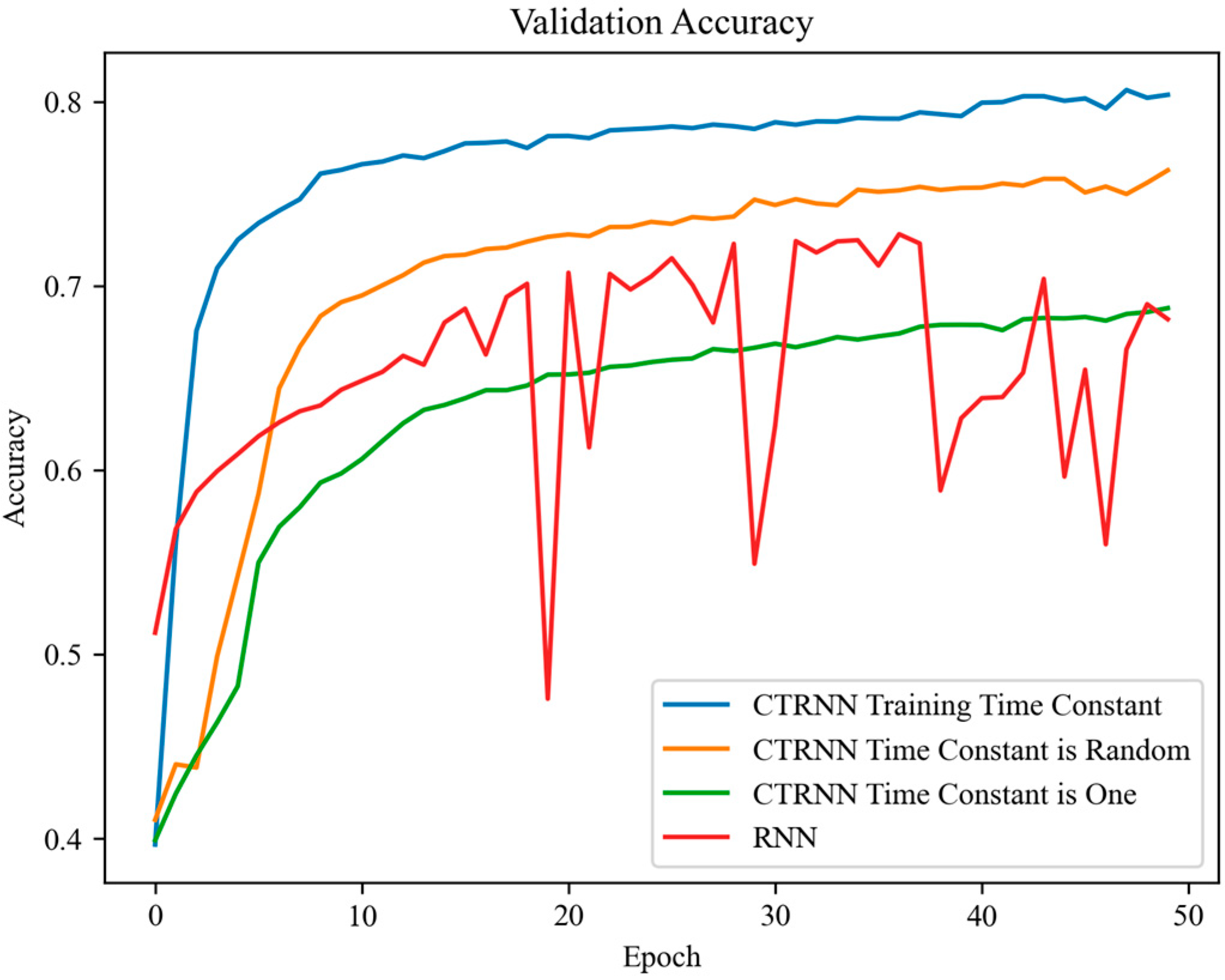
Figure 1. Structure of a Continuous Time Recurrent Neuron (CTRNN): (a) differential equation representation; (b) using a MEMS dynamic.
Applsci 15 07508 g001
Figure 2. WISDM dataset activities, walking and jogging counts, represent more than 50% of the data.
Applsci 15 07508 g002
Figure 3. Model architecture: The input consists of 3 acceleration features: X, Y, and Z. The interconnected recurrent layer contains 16 cells (256 interconnections), followed by a dense layer with 10 cells, and an output layer with 6 cells.
Applsci 15 07508 g003
Figure 4. Forward and backward steps of implementing the CTRNN with time constant as a learnable parameter using the TensorFlow library.
Applsci 15 07508 g004
Figure 5. Validation dataset accuracy for different G-CTRNN configurations and RNN model: the training time constant is the best, random initialization is the second best, and static time constant is the worst, compared to the RNN, which suffers from catastrophic forgetting.
Applsci 15 07508 g005
Table 1. Different G-CTRNN configuration runs and results of ten independent runs.
G-CTRNN ModelAccuracy %
Static time constant equals one68.2 ± 0.6
Random-initialization time constant76.1 ± 2.1
Training the time constant81.9 ± 1.4
Table 2. Comparison of G-CTRNN and RNN parameter sizes and accuracies of ten independent runs.
G-CTRNN Model (Recurrent Cells)Network Parameters SizeAccuracy %
G-CTRNN (16)57281.9 ± 1.4
RNN (32)154881.4 ± 1.2
G-CTRNN (4)15671.8 ± 1.1
RNN (16)55673.1 ± 0.9
Disclaimer/Publisher’s Note: The statements, opinions and data contained in all publications are solely those of the individual author(s) and contributor(s) and not of MDPI and/or the editor(s). MDPI and/or the editor(s) disclaim responsibility for any injury to people or property resulting from any ideas, methods, instructions or products referred to in the content.

