Debris Flow Susceptibility Prediction Using Transfer Learning: A Case Study in Western Sichuan, China

Abstract

The complex geological environment in western Sichuan, China, leads to frequent debris flow disasters, posing significant threats to the lives and property of local residents. In this study, debris flow susceptibility models were developed using three machine learning algorithms: Support Vector Machine (SVM), Random Forest (RF), and Extreme Gradient Boosting (XGBoost). The models were trained with data in Songpan County and used for debris flow susceptibility prediction in Mao County, using small watersheds as assessment units. Seventeen key feature factors based on multi-source remote sensing data encompassing topography and geomorphology, geological structures, environmental elements, and human activities were selected as input parameters after assessment with Pearson correlation analysis. Model performance was rigorously evaluated through ten-fold cross-validation, and hyperparameter optimization was employed to enhance predictive accuracy. To assess the models’ robustness, the trained models were applied to the neighboring Mao County for cross-regional validation. The results consistently indicate that elevation, seismic nucleation density, population density, and distance to roads are the primary controlling factors influencing susceptibility. Comparative analysis between the Songpan and Mao County reveals that the RF model significantly outperforms SVM and XGBoost in accuracy and robustness. Therefore, the RF model is better suited for debris flow susceptibility assessment in western Sichuan. Although the effectiveness of this model may be limited by the relatively small sample size of debris flow events in the dataset and potential variations in environmental conditions across different regions, it still holds promise for providing a scientific basis and decision-making support for disaster mitigation in comparable areas of western Sichuan.

1. Introduction

Debris flows are a common geological hazard characterized by their sudden onset, destructive power, and wide-ranging impacts, often posing severe threats to human lives, property, and ecological systems [1]. Accurately predicting the spatial distribution and susceptibility of debris flows is not only a critical focus of disaster prevention and mitigation, but also an urgent scientific challenge in susceptibility assessment [2].

Traditionally, debris flow susceptibility evaluations have relied on subjective experience and statistical methods, often complemented by remote sensing and geographic information system (GIS) analyses. For single-channel debris flows, field investigations and numerical simulations are typically employed to delineate deposition areas [3]. For regional-scale assessments, susceptibility mapping is generally conducted using GIS-based statistical analyses combined with regional background data and remote sensing imagery. Despite their foundational contributions, traditional methods have demonstrated limitations in complex geological environments and large-scale assessments. Field investigations and expert-driven approaches are constrained by human resources and time efficiency, making the comprehensive coverage of large areas challenging. Moreover, qualitative methods, such as the Analytic Hierarchy Process (AHP) [4,5], rely heavily on expert judgment, resulting in subjective and arbitrary evaluation outcomes [6,7]. Statistical methods, including Weight of Evidence [8,9] and Frequency Ratio [10,11], struggle to capture nonlinear interactions among terrain, geology, hydrology, and other environmental factors [12]. Additionally, numerical simulations demand high-quality data and computational resources, encountering bottlenecks in efficiency and precision when processing large-scale remote sensing datasets.

In recent years, advancements in remote sensing and artificial intelligence have led to the growing adoption of machine learning algorithms in debris flow susceptibility assessments. In this context, algorithms such as logistic regression [13,14], Bayesian models [15,16], convolutional neural networks [17,18], Support Vector Machines [19], Random Forests [20,21,22], and Extreme Gradient Boosting (XGBoost) [23,24,25] have gained popularity. Compared to traditional models, machine learning methods offer advantages such as the ability to handle large datasets, strong generalization capabilities, efficient modeling processes, and higher predictive accuracy [26]. These methods can effectively capture the nonlinear relationships between debris flow susceptibility and environmental factors [27]. Consequently, machine learning algorithms often outperform traditional statistical models and are widely used in debris flow susceptibility evaluations [28].

The western Sichuan region of China is highly susceptible to debris flow disasters due to the combined influences of monsoonal circulation, high-energy terrain, and heterogeneous underlying surface conditions. In recent years, improvements in transportation infrastructure and the rapid growth of tourism have significantly enhanced regional accessibility while simultaneously exerting considerable pressure on the ecological environment [29,30,31]. Large-scale construction activities, transportation infrastructure development, and tourism have led to the destruction of vegetation and soil degradation. Unmanaged mining pits, quarries, and waste disposal sites have provided abundant sources of debris material, exacerbating the occurrence of debris flows [32,33]. Although numerous studies have been conducted on debris flow susceptibility in this region, most have focused on specific areas [34,35,36], limiting their applicability to broader contexts. Some studies have evaluated susceptibility at larger scales, such as Sichuan Province or the upper Minjiang River basin [37,38,39,40], but their coarse spatial resolution often fails to provide detailed guidance for disaster prevention and mitigation efforts.

This study aims to develop a debris flow susceptibility evaluation model with fine-scale resolution and strong generalization capabilities. Songpan County was selected as the study area, with small watersheds serving as the evaluation units. Through Pearson correlation analysis, 17 key conditioning factors were identified across four dimensions: topography, geological structures, environmental factors, and human activities. Three machine learning algorithms—Support Vector Machine (SVM), Random Forest (RF), and Extreme Gradient Boosting (XGBoost)—were employed to construct debris flow susceptibility models. The models were then applied to the Mao County region to validate their generalization performance. Based on the susceptibility evaluation results from Songpan and Mao County, the optimal model was identified in terms of predictive accuracy and robustness, providing scientific evidence and decision-making support for disaster prevention and mitigation in western Sichuan.

2. Study Area

The study area encompasses Songpan County, located within the influence zone of the Qinghai–Tibet Plateau’s monsoon climate. The distribution of precipitation is highly uneven, with approximately 80% of annual rainfall concentrated during the monsoon season, which is characterized by frequent episodes of intense short-duration rainfall. The topography exhibits a pronounced gradient, with higher elevations in the northwest progressively declining toward the southeast. The region is structurally active, featuring well-developed fault systems and significant neotectonic movements (Figure 1). Consequently, the terrain is rugged, exhibiting deep valley incisions and steep slopes (Figure 2a). Mountainous areas are heavily fragmented, with the widespread development of rockfalls, collapses, and landslides (Figure 2b–d). Moreover, intensive human engineering activities, including open-pit mining and sand extraction, have contributed large volumes of engineering waste (Figure 2e,f). The interplay of these natural and anthropogenic factors results in pronounced debris flow activity throughout the study area (Figure 2g–i).

3. Data and Methods

3.1. Debris Flow Inventory

The spatial dataset of debris flow hazards utilized in this study was sourced from the Resources and Environmental Sciences Data Center of the Chinese Academy of Sciences (http://www.resdc.cn, accessed on 2 May 2025). The data are provided in vector SHAPE file format, with attribute fields encompassing hazard type, geographic coordinates, morphological characteristics, and magnitude classifications. Through integration with field-based investigations, a total of 44 debris flow hazard points were confirmed within the Songpan study area. Concurrently, a multi-source spatial dataset from the same platform was compiled, encompassing the ALOS Digital Elevation Model (DEM), road network vector data, land use raster data, geological fault line vectors, seismic hazard point distributions, annual precipitation raster data, soil erosion type and intensity classification rasters, Normalized Difference Vegetation Index (NDVI) raster data, and population spatial distribution. To ensure spatial consistency for modeling, all raster datasets were resampled to a uniform 12.5 m resolution. For detailed information on the dataset types and resolutions, refer to

Table 1. Multi-source spatial dataset summary.

Data Type	Source of Information	Spatial Resolution
Debris Flow Hazard Spatial Dataset	The Resources and Environmental Sciences Data Center of the Chinese Academy of Sciences	Vector data
Digital Elevation Model (DEM)		12.5 m
Road Network Vector Data		Vector data
Land Use Raster Data		30 m
Geological Fault Line Vectors		Vector data
Seismic Hazard Point Distributions		Vector data
Annual Precipitation Raster Data		1 km
Soil Erosion Type and Intensity Classification Rasters		1 km
Normalized Difference Vegetation Index (NDVI) Raster Data		250 m
Population Spatial Distribution		1 km

.

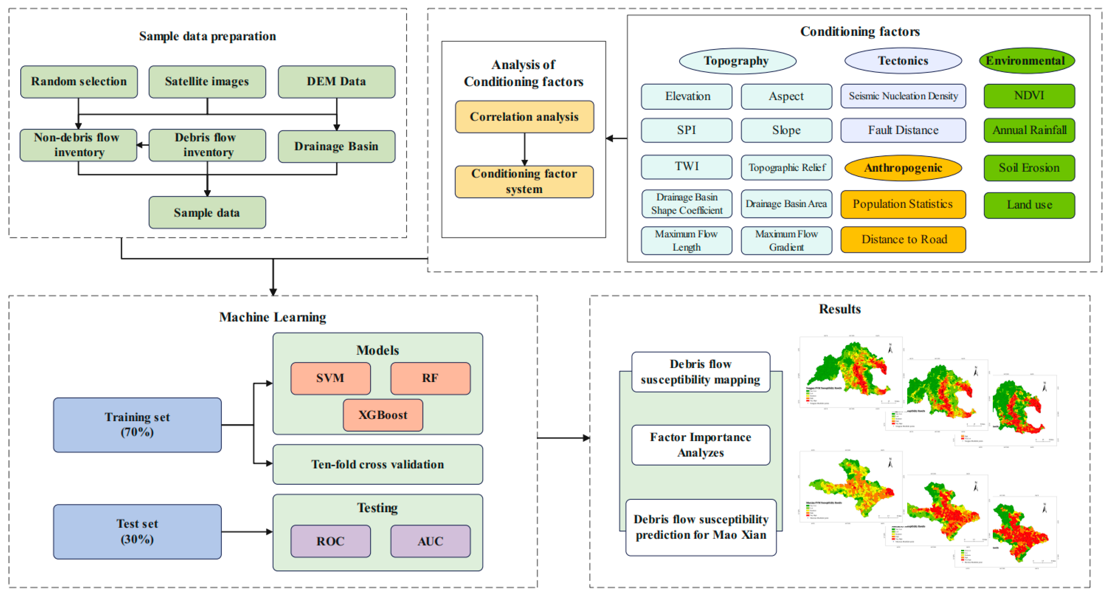
3.2. Susceptibility Assessment Process

The technical workflow of this study illustrated in Figure 3 comprises four main steps, as follows: (1) preparation of the sample data; (2) construction of the susceptibility evaluation factor dataset; (3) application and evaluation of machine learning models; and (4) generation of the debris flow susceptibility map.

3.3. Sample Data Preparation

Current evaluation units for debris flow susceptibility assessment are primarily categorized into two paradigms: grid-based units, and watershed-based units [41]. Grid-based units rely on regular grid matrices, offering advantages such as high data compatibility and computational efficiency within GIS platforms [42,43]. However, their discrete nature limits their ability to systematically represent the overall watershed response mechanisms underlying debris flow initiation. In contrast, watershed-based units are delineated based on geomorphological features, reflecting the natural evolution of the environment and the differentiated boundaries between geomorphology and geology. This makes them more consistent with the actual developmental characteristics of debris flows [44,45,46]. Therefore, in this study, watershed units were extracted using GIS-based spatial analysis techniques applied to a Digital Elevation Model (DEM). By dynamically adjusting the catchment area threshold based on high-resolution remote sensing imagery, a total of 1433 debris flow susceptibility evaluation units were delineated.

Research indicates that susceptibility assessment performs optimally when the number of hazard points and non-hazard points is balanced [47]. To construct the sample dataset, several watershed units were randomly selected, excluding confirmed positive samples. From the remaining units, rigorous validation via visual interpretation of high-resolution satellite imagery was conducted to ensure the absence of debris flow morphological features, severe erosion signs, or historical disaster traces. Additionally, a buffer distance was maintained between these points and known hazard sites to avoid potential active zones. Ultimately, 44 non-hazard watershed units were identified as negative samples. This comprehensive approach ensured that the selected non-hazard points represented stable areas with extremely low debris flow susceptibility in the study region.

This resulted in a dataset comprising 88 samples for debris flow susceptibility analysis (Figure 4). The sample dataset was divided into training (70%) and validation (30%) subsets. To mitigate the risk of overfitting due to the limited sample size, which could restrict the effective utilization of data [48,49], ten-fold spatial clustering cross-validation was applied to the training data, with model hyperparameters optimized accordingly [50]. Spatial clustering was performed using the K-means algorithm [51], which provides better spatial transferability compared to random splitting [52].

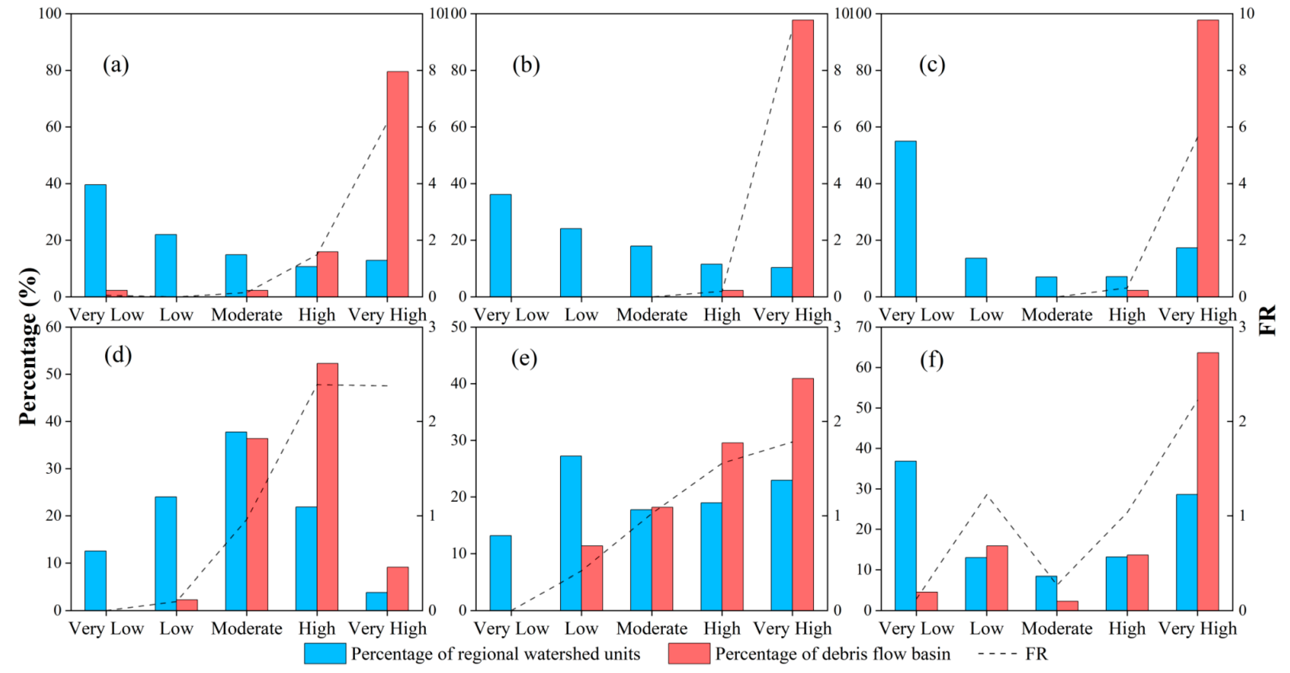
3.4. Conditioning Factors

The occurrence of natural disasters is often the result of the combined effects of multiple factors, including topography, geology, meteorology, and hydrology [53,54,55]. Drawing on previous studies and empirical findings [56,57,58,59,60,61,62,63,64,65,66,67,68], this study selected 18 conditional factors from four categories—topography and geomorphology, geological structures, environmental elements, and human activities—to construct a comprehensive susceptibility factor system.

(1)

Topography: This includes elevation, slope, aspect, topographic wetness index, stream power index, topographic relief, drainage basin shape coefficient, drainage basin area, maximum flow length, and maximum flow gradient. Elevation influences geomorphological and geological evolution, shaping the natural disaster background and indirectly regulating the spatial distribution of human activities. Slope is highly related to the formation and development of debris flows, with suitable slopes facilitating their initiation. Aspect affects microclimatic conditions, which in turn influence vegetation and rock weathering, controlling material availability. The topographic wetness index describes how terrain controls runoff generation and saturation source areas. The stream power index reflects the erosive force of flowing water. Topographic relief indicates the degree of surface erosion and tectonic activity. The drainage basin shape coefficient, drainage basin area, maximum flow length, and maximum flow gradient are the basic parameters for calculating flow paths and velocities, determining debris flow probability and scale.

(2)

Geology. This includes seismic nucleation density and fault distance. Earthquakes and tectonic faults weaken rock and soil strength, producing loose material that serves as debris flow sources.

(3)

Environmental factors. These include the normalized difference vegetation index, soil erosion, land use, and annual rainfall. The normalized difference vegetation index reflects vegetation cover, which promotes soil and water conservation and reduces debris flow sources. Soil erosion indicates surface susceptibility to erosion. Land use alters runoff and infiltration processes, potentially triggering debris flows. Annual rainfall is one of the primary triggers for debris flow events.

(4)

Human activities. These include distance to road and population statistics. Road construction along riverbanks can induce slope instability and accelerate loose material accumulation, raising debris flow risk. Population statistics reflect human activity intensity but are often highest in flatter areas, where geological conditions tend to inhibit debris flow development.

To avoid multicollinearity, the Pearson correlation coefficient was used to analyze the factors. A Pearson coefficient close to 1 indicates a strong positive correlation between two controlling factors, while a coefficient near 0 suggests independence [69]. Previous studies have indicated that a Pearson coefficient exceeding 0.7 may lead to multicollinearity issues [70]. The analysis revealed a very strong positive correlation between slope and terrain roughness (PCC = 0.974) (Figure 5). Given the well-established dominance of slope as a driving factor in surface processes [71], slope was retained, and terrain roughness was excluded. This resulted in the establishment of a debris flow susceptibility evaluation factor system comprising 17 independent factors (Figure 6), which were classified into five levels, as detailed in

Table 2. Classification of conditioning factors.

Conditioning Factors	Very Low	Low	Moderate	High	Very High
Elevation (m)	1009.10–2416.90	2416.90–3120.80	3120.80–3578.33	3578.33–3983.07	3983.08–5496.46
Slope (°)	0–14	14–24	24–32	32–43	43–86
Topographic Wetness Index	0–4	4–6	6–9	9–14	14–33
Stream Power Index	0–4.0 × 103	4.0 × 103–1.0 × 104	1.0 × 104–5.0 × 104	5.0 × 104–1.0 × 106	1.0 × 106–8.66 × 107
Drainage Basin Shape Coefficient	0–0.25	0.25–0.5	0.5–0.75	0.75–1	1–478
Drainage Basin Area (km2)	0–2.47	2.47–5.61	5.61–9.59	9.59–16.09	16.09–45.96
Maximum Flow Length (km)	0–2.50	2.50–4.26	4.26–6.05	6.05–8.85	8.85–17.53
Maximum Flow Gradient	0–0.127	0.127–0.204	0.204–0.293	0.29–0.401	0.401–0.732
Seismic Nucleation Density	4.4 × 10−5–4.8 × 10−5	4.9 × 10−5–5.1 × 10−5	5.2 × 10−5–5.4 × 10−5	5.4 × 10−5–5.6 × 10−5	5.6 × 10−5–5.7 × 10−5
Fault Distance (km)	0–4	4–10	10–16	16–22	22–30
Normalized Difference Vegetation Index	0.082–0.410	0.411–0.596	0.597–0.729	0.730–0.808	0.809–0.912
Soil Erosion (kg/m2/a)	0.015–12.94	12.94–42.02	42.02–87.26	87.26–166.42	166.42–411.99
Annual Rainfall (mm)	685.31–734.83	734.83–758.33	758.33–790.23	790.23–826.32	826.32–899.34
Population Statistics (person/km2)	0–2	2–10	10–30	30–70	70–214
Distance to Road (km)	0–3	3–8	8–13	13–22	22–39

.

3.5. Overview of Machine Learning Models

This study selects Support Vector Machine (SVM), Random Forest (RF), and eXtreme Gradient Boosting (XGBoost) as core modeling algorithms based on three key considerations. First, these algorithms are mature models long validated in geological hazard studies, leveraging standardized implementations from open-source frameworks (e.g., scikit-learn, XGBoost). Their efficient computational performance and integrated hyperparameter optimization tools reduce engineering application thresholds and facilitate model deployment. Second, given the limited dataset with only 44 debris flow hazard positive samples, SVM constructs margin-maximizing decision boundaries via kernel mapping in high-dimensional spaces, while RF and XGBoost mitigate overfitting through Bagging ensembles and gradient boosting iterations, respectively. Third, these algorithms represent distinct machine learning paradigms: although SVM lacks native feature importance metrics, it enables contribution quantification via SHAP values, whereas RF and XGBoost directly output importance rankings based on Gini impurity reduction and split gain mechanisms, providing multi-dimensional interpretability for debris flow susceptibility analysis.

In recent years, ensemble learning strategies have gained popularity in machine learning applications, enhancing predictive performance by fusing the advantages of multiple base models. For instance, a study on seismic risk assessment of reinforced concrete shear walls [72] proposes stacked machine learning (Stacked ML) models integrated with Bayesian optimization (BO), genetic algorithms (GA), and other optimization strategies. This approach provides a new paradigm for structural seismic performance analysis in complex feature spaces by integrating base algorithms with intelligent parameter optimization. While such ensemble optimization demonstrates predictive advantages in high-dimensional scenarios, this study prioritizes classical algorithms like SVM and RF for their interpretability and computational efficiency in transfer learning contexts.

3.5.1. Random Forest

Random Forest (RF) is an ensemble algorithm composed of multiple decision trees [73,74]. This method employs bagging to generate k decision trees, each constructed using a bootstrap-sampled training subset. At each node split, a random subset of m features is selected. The final prediction is integrated through majority voting for classification tasks or mean regression for regression tasks. The output of the RF is the class with the highest average probability across all decision trees, as calculated by Equation (1).

$$p_c=\max \left\{p_i={\displaystyle \frac{{\displaystyle \sum _{j=1}^m{p}_{ij}}}{m}}\left|i\in I\right.\right\}$$

(1)

In this equation, I is the set of all classifications; m is the number of decision trees; p_i is the probability of an event occurring or existing; p_ij is the probability of the event occurring or existing in the j-th decision tree; p_c is the probability corresponding to the class chosen by the model.

3.5.2. Support Vector Machine

Support Vector Machine (SVM) is a machine learning method based on the principle of structural risk minimization, offering a superior generalization ability compared to other conventional methods [75]. SVM possesses several unique advantages in addressing nonlinear, high-dimensional pattern recognition problems. The algorithm supports four types of kernel functions: linear, polynomial, sigmoid, and radial basis function (RBF). The literature indicates that, among these kernels, the RBF kernel provides better performance in predicting hazard susceptibility [76]. The decision function of the RBF-SVM is presented in Equation (2).

$$f\left(x\right)=sign\left({\displaystyle \sum _{i=1}^n{a}_i}{y}_i\exp (-{\displaystyle \frac{‖x_i-x‖}{2{\sigma }^2}})+b\right)$$

(2)

In the equation, x_i is the influence factor vector of the training sample; y_i is the class label of the sample; α_i is the Lagrange multiplier; x is the influence factor vector of the sample to be predicted; σ controls the decay of the RBF kernel function, with a larger value leading to the faster decay and lower dimensionality of the feature mapping; and b is the intercept.

3.5.3. Extreme Gradient Boosting

XGBoost, also known as Extreme Gradient Boosting, is an ensemble algorithm based on classification or regression trees, which has demonstrated excellent performance in Kaggle competitions [77]. The model incorporates several innovative strategies such as parallel processing, column subsampling, and dynamic learning rate adjustment. These techniques not only maintain computational efficiency but also effectively mitigate overfitting. Moreover, its distributed computing framework enables rapid training on large-scale datasets. The objective function of the model is shown in Equation (3).

$$J\left(f_t\right)={\displaystyle \sum _{i=1}^{n}L}\left(y_i,{\widehat{y}}^{\left(t-1\right)}+f_t\left(x_i\right)\right)+\mathsf{\Omega }\left(f_t\right)+C$$

(3)

In this equation, i represents the i-th sample, y_i represents the true value of the i-th sample, y^(t−1) represents the predicted value of the i-th sample from the (t − 1) iteration model, ft_(xi) represents the new model added at the t-th iteration, Ω(ft) represents the regularization term, C represents some constant terms, and the outermost L() represents the overall objective function.

3.5.4. Model Accuracy Verification

To systematically evaluate the prediction accuracy and robustness of three debris flow susceptibility models, this study employs the Receiver Operating Characteristic (ROC) curve and the Area Under the Curve (AUC) to quantify model performance. Additionally, the Frequency Ratio (FR) index is utilized to validate the spatial rationality of the prediction results.

The ROC curve is widely recognized as an effective method for assessing the accuracy of debris flow susceptibility evaluation [78]. It plots the True Positive Rate (TPR) on the vertical axis against the False Positive Rate (FPR) on the horizontal axis. The AUC value ranges from 0 to 1, with higher values indicating better model performance. The classification criteria for AUC values are as follows: excellent (0.9–1), very high (0.8–0.9), good (0.7–0.8), moderate (0.6–0.7), or poor (0.5–0.6) [79].

The Frequency Ratio (FR) is an index used to characterize the distribution of debris flow watersheds within specific risk zones. It is calculated as the ratio of the proportion of debris flow disaster points within a given risk level to the proportion of all watershed units within the same risk level [80]. According to the literature, regions with higher susceptibility values should encompass as many disaster points as possible while occupying the smallest possible area [81]. Furthermore, the FR value should increase with higher susceptibility levels [82].

4. Results

4.1. Hyperparameter Optimization

Hyperparameter optimization is a crucial step in enhancing the performance of machine learning models. Default hyperparameter settings often fail to fully exploit the potential of algorithms. To ensure optimal predictive performance, the systematic tuning of hyperparameters is necessary prior to formal training [83]. Notably, while grid search was employed for its deterministic exhaustiveness, this study acknowledges the potential of the novel optimization methods proposed in [72], which adaptively explore hyperparameter spaces using probabilistic models or evolutionary strategies. These methods may offer more efficient global optimization in large datasets. However, we prioritized grid search here for its reproducibility and computational tractability. The hyperparameter search spaces were determined through a systematic integration of literature-based benchmarks, framework recommendations, pre-experimental validation, and computational feasibility. The defined ranges thus strike a balance between empirical effectiveness and practical implementation, ensuring both model performance and computational efficiency for the debris flow dataset.

Model performance under different parameter combinations is assessed using ten-fold cross-validation, leading to the selection of optimized parameter configurations [84].

Table 3. Tuned hyperparameters in each classifier model.

Model	Hyperparameter	Definition	Optimum
SVM	C	Regularization parameter that controls the trade-off between achieving a low error and keeping the model simple. Higher values reduce bias but may increase variance.	10
	gamma	Defines how far the influence of a single training example reaches. A lower value means a larger influence region.	scale
	kernel	Specifies the kernel type to be used in the algorithm, affecting decision boundaries.	RBF
RF	n_estimators	The number of trees in the forest. More trees generally improve performance but increase computation time.	200
	max_depth	The maximum depth of each decision tree. If none, nodes are expanded until all leaves are pure.	10
	min_samples_split	The minimum number of samples required to split an internal node. Higher values prevent overfitting.	2
	min_samples_leaf	The minimum number of samples required to be at a leaf node. Higher values make the model more robust.	1
XGBoost	n_estimators	The number of boosting rounds. More rounds can improve performance but may lead to overfitting.	100
	max_depth	Maximum depth of a tree. Larger values capture more patterns but increase complexity.	6
	learning_rate	Controls the step size in updating weights. Lower values lead to slower but more stable convergence.	0.2
	subsample	Fraction of training samples used in each boosting iteration to prevent overfitting.	1.0

presents the key hyperparameters and their optimal values for each classifier. Based on the selected optimal parameter combinations, all classifiers were retrained to ensure stability and a generalization capability.

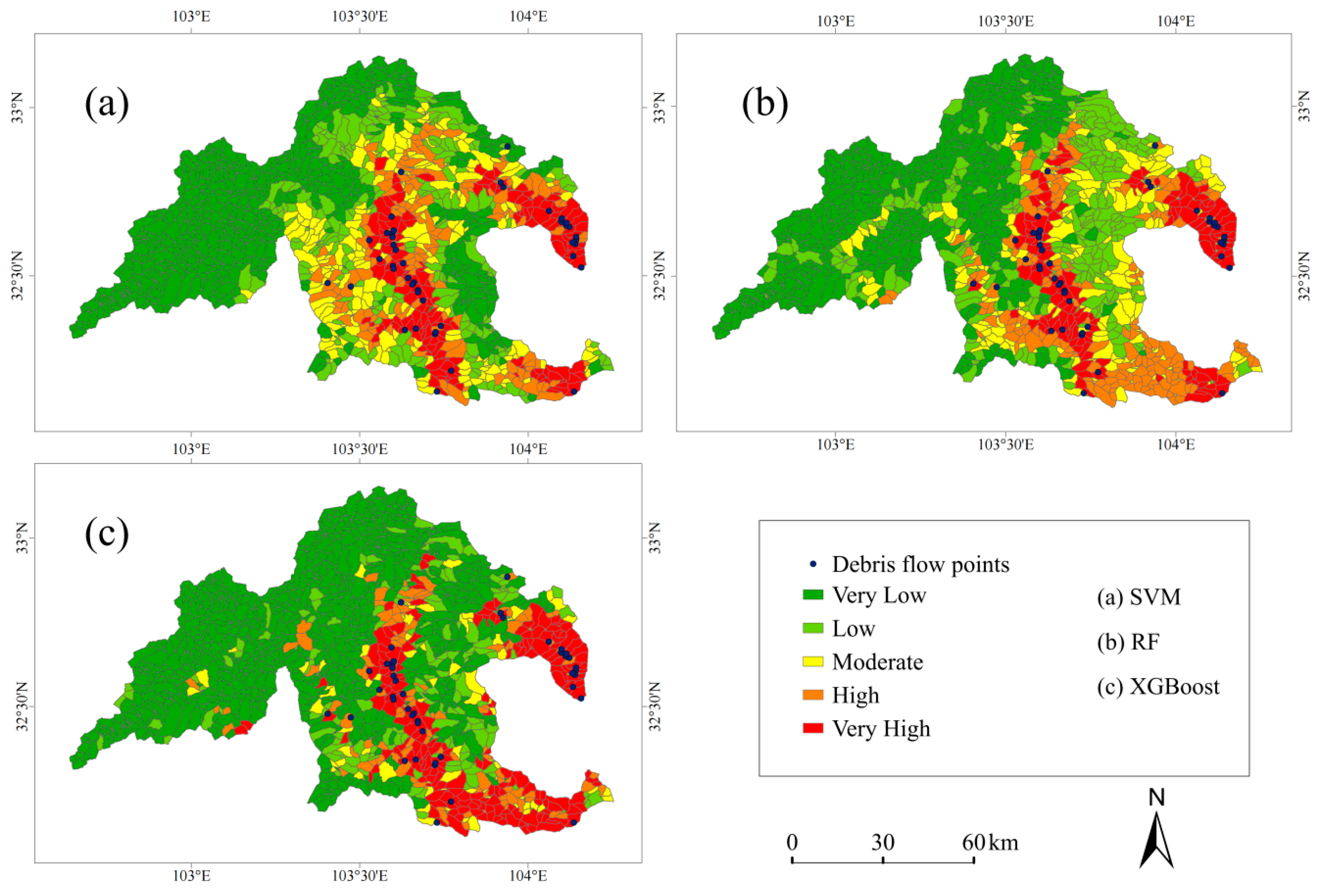
4.2. Debris Flow Susceptibility Mapping in Songpan

The results of the landslide susceptibility assessment for the Songpan region were classified into five susceptibility levels (very high, high, medium, low, and very low) using the Jenks natural breaks classification method. As shown in Figure 7, the high-susceptibility areas of landslides exhibit a clear spatial clustering pattern, predominantly distributed in the central, southern, and northeastern–southeastern transitional zones of the study area, while the low-susceptibility areas are mainly located in the northwestern plateau region. The results show a high degree of concordance with the spatial distribution of landslide disaster points, thus validating the scientific and reliable nature of the assessment method employed in this study.

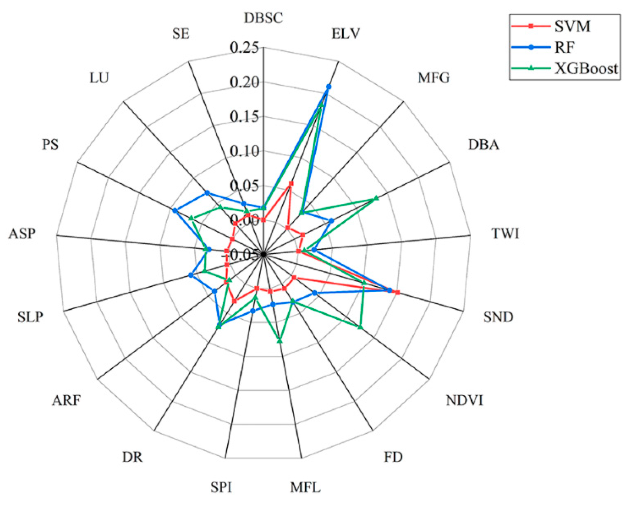
4.3. Factor Importance

In the study of debris flow susceptibility modeling in the Songpan region, feature importance for RF and XGBoost was calculated using their respective built-in methods. For RF, this involved Gini importance based on the mean decrease in impurity, while XGBoost utilized gain importance to reflect split contributions. Given that SVM does not directly provide feature importance metrics, SHAP (SHapley Additive exPlanations) values were employed for this model. SHAP quantifies feature importance using game theory principles to determine each feature’s contribution to model predictions.

Due to the differing measurement scales and principles across algorithms, all raw importance values were normalized to the [0, 1] interval using Min-Max scaling. The comprehensive importance ranking presented in Figure 8 is derived from the arithmetic mean of the normalized values across the three models (RF, XGBoost, and SVM-SHAP). This approach ensures cross-model comparability and enables an integrated prioritization of features.

The results indicate that elevation, earthquake kernel density, population density, and distance to roads significantly influence debris flow susceptibility in the study area, which is consistent with findings from previous studies [85,86].

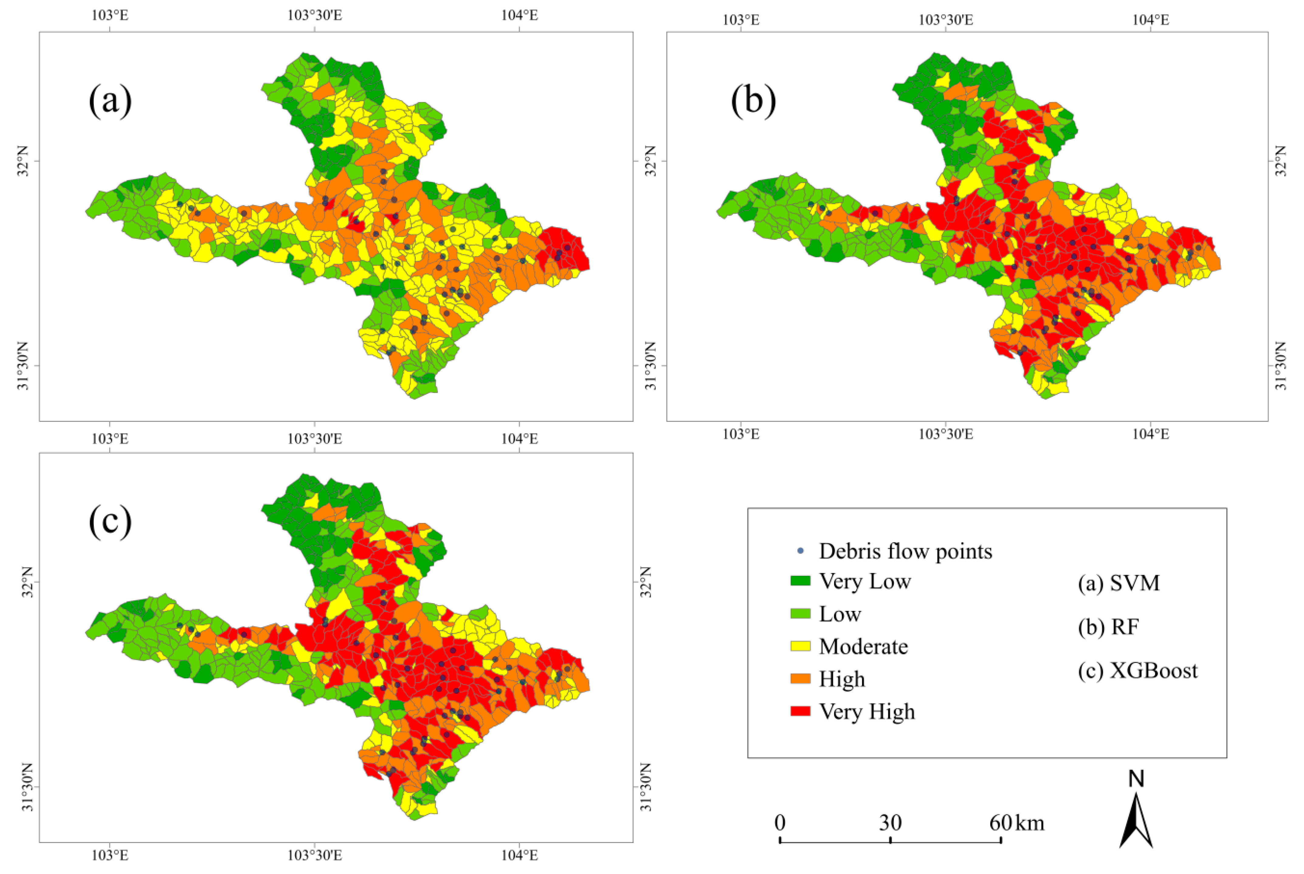
4.4. Debris Flow Susceptibility Mapping in Mao County

To validate the robustness of the landslide susceptibility model, and given the geological, topographical, and climatic similarities between Songpan and Mao County, as well as the common mechanisms operating within landslide disasters, this study applied the modeling results from the Songpan region to Mao County for landslide susceptibility mapping. Figure 9 shows that the high-susceptibility areas in Mao County are concentrated in the central fault basin and the deep-cut river valleys in the south, extending in a band-like distribution along the eastern fault zone. The low-susceptibility areas are widely distributed across the western plateau terraces and the northern folded mountainous regions. The results exhibit a high degree of correspondence with the spatial distribution of landslide disaster points, thereby validating the scientific accuracy and reliability of the evaluation methods employed in this study.

5. Discussion

5.1. Factor Importance Analysis

The region is characterized by intense tectonic activity, significant topographical cutting, and steep mountainous landforms, with an average slope greater than 25° on most slopes. Due to river erosion controlling the base level, human activities are concentrated in relatively flat, low-altitude valley areas. Current landslide surveys mainly serve disaster prevention and mitigation needs, with survey areas often focused on valleys with engineering facilities or population concentrations. These areas typically have high accessibility and are located close to roads. In contrast, remote valleys with poor transportation conditions and no protective structures are often excluded from systematic investigations due to survey costs and engineering benefits. This spatially selective survey approach results in a significant clustering of landslide point data, leading to higher weights for factors such as elevation, population density, and distance to roads in the susceptibility assessment model. Additionally, the high contribution of the seismic nucleation density factor objectively reveals the strong correlation between the spatial distribution of landslide disasters in the region and seismic activity.

5.2. Best Model

Figure 10 presents a comparison of the ROC curves for landslide susceptibility evaluation using three models in the Songpan and Mao County regions. In the Songpan region, all three models demonstrate excellent predictive performance, with the RF model (AUC = 0.917) performing the best, followed by the SVM model (AUC = 0.907) and the XGBoost model (AUC = 0.903). In the Mao County region, the RF model continues to maintain high predictive accuracy (AUC = 0.804), while the accuracy of the SVM (AUC = 0.710) and XGBoost (AUC = 0.766) models has slightly decreased compared to the Songpan region, though they remain at a good level overall.

The Frequency Ratio (FR) values, calculated as the ratio of the percentage of landslide disaster points to the percentage of basin units within each susceptibility class, are shown in Figure 11. In the Songpan region, the SVM model still classifies some landslide points into the very-low-susceptibility class, and their FR values do not increase with the elevation of susceptibility levels. In contrast, the RF and XGBoost models mainly categorize landslide points into the very-high-susceptibility class, with the RF model achieving an FR value of 9.462, which is higher than that of XGBoost (FR = 5.647). This result further confirms the superiority of the RF model in the Songpan region.

In the Mao County region, the FR values for the SVM model increase with the elevation of susceptibility levels, but the number of landslide points classified into the very-high-susceptibility class is very small. XGBoost categorizes the highest number of landslide points into the very-high-susceptibility class, but there are still some landslide points classified into the very-low-susceptibility class, and its FR values do not increase with the elevation of susceptibility levels. In contrast, the RF model does not classify any landslide points into the very-low-susceptibility class, and the number of landslide points in the very-high-susceptibility class is relatively high, with FR values increasing as susceptibility levels rise. This result also validates the superiority of the RF model in the Mao County region.

The superior performance of the Random Forest (RF) model in this study can be attributed to the congruence between its algorithmic characteristics and the dataset’s features. First, given that debris flow susceptibility is governed by complex nonlinear interactions among multiple factors, RF demonstrates efficacy in capturing these intricate patterns. Second, considering the potential redundancy or measurement noise inherent in the 17 input factors, RF’s random feature subset selection (feature bagging) and majority voting decision mechanism endow it with inherent robustness against irrelevant features and noise. Third, RF mitigates model variance through the construction and integration of multiple weak learners, rendering it less susceptible to overfitting and enhancing generalization capability, particularly with a relatively limited sample size of disaster points (n = 44). This advantage stands in contrast to the Support Vector Machine (SVM), which encounters challenges in identifying optimal hyperplanes within high-dimensional spaces with small samples. As a boosting algorithm, XGBoost tends to construct stronger learners but may exhibit elevated variance, thereby harboring a potential risk of overfitting in small-sample scenarios. All models were subjected to grid search for parameter optimization, ensuring that each algorithm was evaluated under its optimal configuration for this specific dataset. The primacy of RF reflects its effective bias–variance trade-off under the data constraints of this study, rather than implying absolute superiority across all contexts.

5.3. Regional Adaptability Challenges in Transfer Learning

The reliance on a limited training dataset in this study may entail multiple methodological challenges. The model’s sensitivity to sample stochasticity increases, whereby extreme values can skew feature importance rankings and potentially misclassify secondary geological factors as key drivers. Additionally, the capacity to identify nonlinear couplings among geological factors is constrained in high-dimensional feature spaces. Small sample sizes also limit model generalization, rendering extrapolation prone to imbalances between overfitting and underfitting, particularly in rare geological scenarios. Although ten-fold cross-validation enhances evaluation stability through iterative sample partitioning, it cannot fully address the fundamental constraint of sample scarcity on model generalization.

Moreover, the disparities between Songpan (source domain) and Mao County (target domain) impose additional challenges for transfer learning. For instance, Songpan has fewer seismic points concentrated in the northeastern direction, while Mao County’s proximity to the Beichuan–Yingxiu and Maowen Fault Zones subjects it to stronger tectonic influence, resulting in a larger number of seismic points that are more dispersedly distributed across its territory. This spatial heterogeneity in seismic activity may disrupt the transferability of fault-related feature associations derived from Songpan’s dataset. Human settlement patterns also exhibit stark contrasts: Songpan’s population is predominantly clustered along central road networks, whereas Mao County has a more evenly distributed population. Such differences in the spatial configuration of human activities introduce unmodeled confounding factors—for example, the model trained on Songpan data may overemphasize the proximity effects of roads and settlements, which diminishes predictive relevance in the context of Mao County’s dispersed settlements.

Collectively, these factors—including the limited training dataset and the pronounced disparities between Songpan and Mao County—likely underlie the observed decline in prediction accuracy for Mao County.

5.4. Limitations and Future Work

This study still has several limitations. Firstly, the automated watershed delineation method based on the digital elevation model (DEM) is constrained by fixed threshold settings, which often result in the fragmentation of complete debris flow gully systems into multiple sub-watershed units. Consequently, the evaluation results may not spatially align well with natural geomorphological entities. Although the manual integration of watersheds using high-resolution remote sensing imagery can effectively improve the integrity of evaluation units, this approach is time-consuming and conflicts with the efficiency advantages of automated modeling. Future research should focus on optimizing the delineation approach and threshold selection [87] to maintain the efficiency of automated extraction while enhancing the spatial consistency between evaluation units and natural geomorphology. This would better represent the integrity of gully systems and balance computational efficiency with spatial analysis accuracy, ultimately providing a more robust evaluation framework for geological hazard assessment in complex terrains.

Secondly, the DEM data used in this study were acquired relatively early and may not accurately capture the dynamic changes in terrain and geomorphology within the study area. Long-term geological processes, climate variations, and human activities can lead to terrain alterations such as mountain erosion and land-use changes, causing discrepancies between DEM-derived terrain features (e.g., slope, aspect, terrain roughness) and current conditions. These discrepancies could potentially impact the accuracy of susceptibility assessments based on these data. Moreover, future work may consider integrating time-series InSAR deformation monitoring and multi-source remote sensing to develop dynamic terrain update models [88], thereby improving data responsiveness to anthropogenic and natural changes.

Thirdly, the random selection method for negative samples applied in this study, while simple, is highly random and vulnerable to human interference, and so it may inadequately cover the characteristics of non-disaster regions. Another commonly used approach is generating negative samples outside buffer zones of positive samples; however, the absence of standardized buffer distances and the difficulty in adapting distance-based delineation to regional specifics may compromise reliability [89]. Furthermore, future research could attempt to use an iterative approach—first conducting susceptibility assessments using random sampling, then selecting negative samples from low-susceptibility areas in the results for a refined evaluation. This iterative process may optimize negative sample selection and enhance the accuracy and reliability of outcomes.

Finally, compared to its performance in the Songpan region, the landslide susceptibility model showed a decline in accuracy during validation in Mao County. To further optimize the model and improve its predictive capability and reliability in different regions, future research could expand the validation case library to include multiple landform types in western Sichuan, providing a comprehensive assessment of the model’s performance in complex and diverse terrain conditions. Additionally, exploring new indicators, such as tourist heat intensity, in the evaluation system could reveal their potential correlation with landslide susceptibility, enhancing the model’s ability to assess debris flow risk in different regions, and providing a more reliable basis for landslide disaster prevention and mitigation.

6. Conclusions

This study conducted a Pearson correlation analysis to select 17 key feature factors from four dimensions: topography, geology, environmental factors, and human activities. Three machine learning models—Support Vector Machine (SVM), Random Forest (RF), and Extreme Gradient Boosting (XGBoost)—were employed to construct a landslide susceptibility model for the Songpan region. The resulting model was then applied to the Mao County region to validate its generalization ability in other study areas. Based on the landslide susceptibility evaluation results for both Songpan and Mao County, the best model was selected based on predictive accuracy and robustness. Finally, an importance ranking of the landslide susceptibility factors was performed. The results indicate the following:

(1)

In the Songpan region, high landslide susceptibility areas are primarily located in the central, southern, and northeast–southeast transition zones of the study area, while low-susceptibility areas are concentrated in the northwest plateau region. In the Mao County region, high-susceptibility areas are concentrated in the central fault basin, southern deeply cut river valleys, and along the eastern fault zone in a strip-like distribution. Low-susceptibility areas are mainly found in the western plateau and northern folded mountains. This spatial distribution pattern highly matches the spatial distribution characteristics of landslide disaster points, thus validating the scientific and reliable evaluation method used in this study.

(2)

The study results highlight the significant influences of factors such as elevation, seismic nucleation density, population density, and distance to roads on landslide susceptibility, further revealing the main controlling factors of landslide disasters in the region.

(3)

Compared to the Support Vector Machine model and Extreme Gradient Boosting model, the Random Forest model demonstrated better applicability in both the Songpan and Mao County regions. It exhibited greater advantages in landslide susceptibility prediction tasks and is a more suitable choice for landslide susceptibility analysis in the complex geological environment of western Sichuan. This provides a cross-regional adaptive technical framework and quantitative evaluation paradigm for risk prevention and control in typical geological disaster-prone areas, such as active regions influenced by monsoon climates.

The debris flow susceptibility maps generated by this study provide spatial decision-making support for local disaster management authorities (e.g., natural resource bureaus and emergency management agencies). High-susceptibility zones should be designated as avoidance areas for land-use planning and infrastructure development, requiring implementation of stringent engineering control measures when construction is unavoidable. These areas warrant prioritized installation of specialized monitoring equipment (e.g., rainfall gauges, debris flow detectors, video surveillance systems) and community-based monitoring networks. The zoning results enable the formulation of granular emergency response plans at township levels, with explicit delineation of evacuation routes and shelter locations tailored to different risk classifications. Furthermore, these zoning maps should be integrated into public awareness campaigns to enhance risk perception and self-rescue capabilities among residents in high-risk areas. The transfer learning framework employed in this research holds promise for application in analogous geological settings throughout southwestern Sichuan, providing robust technical support for regional geohazard risk assessment and disaster prevention initiatives.

References

1. Dias, H.C.; Hölbling, D.; Grohmann, C.H. Landslide Susceptibility Mapping in Brazil: A Review. Geosciences 2021, 11, 425. [Google Scholar] [CrossRef]
2. Liu, Y.; Chen, J.; Sun, X.; Li, Y.; Zhang, Y.; Xu, W.; Yan, J.; Ji, Y.; Wang, Q. A progressive framework combining unsupervised and optimized supervised learning for debris flow susceptibility assessment. CATENA 2024, 234, 107560. [Google Scholar] [CrossRef]
3. Li, Y.-m.; Su, L.-j.; Zou, Q.; Wei, X.-l. Risk assessment of glacial debris flow on alpine highway under climate change: A case study of Aierkuran Gully along Karakoram Highway. J. Mt. Sci. 2021, 18, 1458–1475. [Google Scholar] [CrossRef]
4. Hossain, M.N.; Mumu, U.H. Flood susceptibility modelling of the Teesta River Basin through the AHP-MCDA process using GIS and remote sensing. Nat. Hazards 2024, 120, 12137–12161. [Google Scholar] [CrossRef]
5. Zhang, G.; Cai, Y.; Zheng, Z.; Zhen, J.; Liu, Y.; Huang, K. Integration of the Statistical Index Method and the Analytic Hierarchy Process technique for the assessment of landslide susceptibility in Huizhou, China. CATENA 2016, 142, 233–244. [Google Scholar] [CrossRef]
6. Dash, R.K.; Falae, P.O.; Kanungo, D.P. Debris flow susceptibility zonation using statistical models in parts of Northwest Indian Himalayas—Implementation, validation, and comparative evaluation. Nat. Hazards 2022, 111, 2011–2058. [Google Scholar] [CrossRef]
7. Tayyab, M.; Hussain, M.; Zhang, J.; Ullah, S.; Tong, Z.; Rahman, Z.U.; Al-Aizari, A.R.; Al-Shaibah, B. Leveraging GIS-based AHP, remote sensing, and machine learning for susceptibility assessment of different flood types in peshawar, Pakistan. J. Environ. Manag. 2024, 371, 123094. [Google Scholar] [CrossRef]
8. Chen, W.; Panahi, M.; Tsangaratos, P.; Shahabi, H.; Ilia, I.; Panahi, S.; Li, S.; Jaafari, A.; Ahmad, B.B. Applying population-based evolutionary algorithms and a neuro-fuzzy system for modeling landslide susceptibility. CATENA 2019, 172, 212–231. [Google Scholar] [CrossRef]
9. Youssef, A.M.; Pourghasemi, H.R.; El-Haddad, B.A.; Dhahry, B.K. Landslide susceptibility maps using different probabilistic and bivariate statistical models and comparison of their performance at Wadi Itwad Basin, Asir Region, Saudi Arabia. Bull. Eng. Geol. Environ. 2016, 75, 63–87. [Google Scholar] [CrossRef]
10. Huang, F.; Yan, J.; Fan, X.; Yao, C.; Huang, J.; Chen, W.; Hong, H. Uncertainty pattern in landslide susceptibility prediction modelling: Effects of different landslide boundaries and spatial shape expressions. Geosci. Front. 2022, 13, 101317. [Google Scholar] [CrossRef]
11. Esper Angillieri, M.Y. Debris flow susceptibility mapping using frequency ratio and seed cells, in a portion of a mountain international route, Dry Central Andes of Argentina. CATENA 2020, 189, 104504. [Google Scholar] [CrossRef]
12. Ahmed, B.; Dewan, A. Application of Bivariate and Multivariate Statistical Techniques in Landslide Susceptibility Modeling in Chittagong City Corporation, Bangladesh. Remote Sens. 2017, 9, 304. [Google Scholar] [CrossRef]
13. Li, J.; Chen, Y.; Jiao, J.; Chen, Y.; Chen, T.; Zhao, C.; Zhao, W.; Shang, T.; Xu, Q.; Wang, H.; et al. Gully erosion susceptibility maps and influence factor analysis in the Lhasa River Basin on the Tibetan Plateau, based on machine learning algorithms. CATENA 2024, 235, 107695. [Google Scholar] [CrossRef]
14. Li, Y.; Chen, J.; Tan, C.; Li, Y.; Gu, F.; Zhang, Y.; Mehmood, Q. Application of the borderline-SMOTE method in susceptibility assessments of debris flows in Pinggu District, Beijing, China. Nat. Hazards 2021, 105, 2499–2522. [Google Scholar] [CrossRef]
15. Pourghasemi, H.R.; Rahmati, O. Prediction of the landslide susceptibility: Which algorithm, which precision? CATENA 2018, 162, 177–192. [Google Scholar] [CrossRef]
16. Youssef, A.M.; Pourghasemi, H.R. Landslide susceptibility mapping using machine learning algorithms and comparison of their performance at Abha Basin, Asir Region, Saudi Arabia. Geosci. Front. 2021, 12, 639–655. [Google Scholar] [CrossRef]
17. Chou, T.-Y.; Hoang, T.-V.; Fang, Y.-M.; Nguyen, Q.-H.; Lai, T.A.; Pham, V.-M.; Vu, V.-M.; Bui, Q.-T. Swarm-based optimizer for convolutional neural network: An application for flood susceptibility mapping. Trans. GIS 2021, 25, 1009–1026. [Google Scholar] [CrossRef]
18. Yi, Y.; Zhang, Z.; Zhang, W.; Jia, H.; Zhang, J. Landslide susceptibility mapping using multiscale sampling strategy and convolutional neural network: A case study in Jiuzhaigou region. CATENA 2020, 195, 104851. [Google Scholar] [CrossRef]
19. Sharma, N.; Saharia, M.; Ramana, G.V. High resolution landslide susceptibility mapping using ensemble machine learning and geospatial big data. CATENA 2024, 235, 107653. [Google Scholar] [CrossRef]
20. Gao, R.; Wang, C.; Wu, D.; Liu, H.; Liu, X. Comprehensive application of transfer learning, unsupervised learning and supervised learning in debris flow susceptibility mapping. Appl. Soft Comput. 2025, 170, 112612. [Google Scholar] [CrossRef]
21. Achour, Y.; Pourghasemi, H.R. How do machine learning techniques help in increasing accuracy of landslide susceptibility maps? Geosci. Front. 2020, 11, 871–883. [Google Scholar] [CrossRef]
22. Gao, R.-y.; Wang, C.-m.; Liang, Z. Comparison of different sampling strategies for debris flow susceptibility mapping: A case study using the centroids of the scarp area, flowing area and accumulation area of debris flow watersheds. J. Mt. Sci. 2021, 18, 1476–1488. [Google Scholar] [CrossRef]
23. Rabby, Y.W.; Hossain, M.B.; Abedin, J. Landslide susceptibility mapping in three Upazilas of Rangamati hill district Bangladesh: Application and comparison of GIS-based machine learning methods. Geocarto Int. 2022, 37, 3371–3396. [Google Scholar] [CrossRef]
24. Shi, X.; Chen, D.; Wang, J.; Wang, P.; Wu, Y.; Zhang, S.; Zhang, Y.; Yang, C.; Wang, L. Refined landslide inventory and susceptibility of Weining County, China, inferred from machine learning and Sentinel-1 InSAR analysis. Trans. GIS 2024, 28, 1594–1616. [Google Scholar] [CrossRef]
25. Zhu, X.; Guo, H.; Huang, J.J. Urban flood susceptibility mapping using remote sensing, social sensing and an ensemble machine learning model. Sustain. Cities Soc. 2024, 108, 105508. [Google Scholar] [CrossRef]
26. Zhang, Y.; Ge, T.; Tian, W.; Liou, Y.-A. Debris Flow Susceptibility Mapping Using Machine-Learning Techniques in Shigatse Area, China. Remote Sens. 2019, 11, 2801. [Google Scholar] [CrossRef]
27. Dou, J.; Yunus, A.P.; Bui, D.T.; Merghadi, A.; Sahana, M.; Zhu, Z.; Chen, C.-W.; Han, Z.; Pham, B.T. Improved landslide assessment using support vector machine with bagging, boosting, and stacking ensemble machine learning framework in a mountainous watershed, Japan. Landslides 2020, 17, 641–658. [Google Scholar] [CrossRef]
28. Shirzadi, A.; Shahabi, H.; Chapi, K.; Bui, D.T.; Pham, B.T.; Shahedi, K.; Ahmad, B.B. A comparative study between popular statistical and machine learning methods for simulating volume of landslides. CATENA 2017, 157, 213–226. [Google Scholar] [CrossRef]
29. Lin, Y.; Jin, Y.; Lin, M.; Wen, L.; Lai, Q.; Zhang, F.; Ge, Y.; Li, B. Exploring the spatial and temporal evolution of landscape ecological risks under tourism disturbance: A case study of the Min River Basin, China. Ecol. Indic. 2024, 166, 112412. [Google Scholar] [CrossRef]
30. Lin, Y.; Hu, X.; Zheng, X.; Hou, X.; Zhang, Z.; Zhou, X.; Qiu, R.; Lin, J. Spatial variations in the relationships between road network and landscape ecological risks in the highest forest coverage region of China. Ecol. Indic. 2019, 96, 392–403. [Google Scholar] [CrossRef]
31. Liu, J.; Wang, J.; Wang, S.; Wang, J.; Deng, G. Analysis and simulation of the spatiotemporal evolution pattern of tourism lands at the Natural World Heritage Site Jiuzhaigou, China. Habitat Int. 2018, 79, 74–88. [Google Scholar] [CrossRef]
32. Zhang, Y.-Q.; Wang, Y.-L.; Li, H.; Li, X.-M. Risk assessment of mountain tourism on the Western Sichuan Plateau, China. J. Mt. Sci. 2023, 20, 3360–3375. [Google Scholar] [CrossRef]
33. Liu, Y.; Peng, J.; Zhang, T.; Zhao, M. Assessing landscape eco-risk associated with hilly construction land exploitation in the southwest of China: Trade-off and adaptation. Ecol. Indic. 2016, 62, 289–297. [Google Scholar] [CrossRef]
34. Cao, J.; Zhang, Z.; Du, J.; Zhang, L.; Song, Y.; Sun, G. Multi-geohazards susceptibility mapping based on machine learning—A case study in Jiuzhaigou, China. Nat. Hazards 2020, 102, 851–871. [Google Scholar] [CrossRef]
35. Li, Y.; Xu, L.; Shang, Y.; Chen, S. Debris Flow Susceptibility Evaluation in Meizoseismal Region: A Case Study in Jiuzhaigou, China. J. Earth Sci. 2024, 35, 263–279. [Google Scholar] [CrossRef]
36. Chen, X.; Chen, H.; You, Y.; Chen, X.; Liu, J. Weights-of-evidence method based on GIS for assessing susceptibility to debris flows in Kangding County, Sichuan Province, China. Environ. Earth Sci. 2015, 75, 70. [Google Scholar] [CrossRef]
37. Xu, W.; Yu, W.; Jing, S.; Zhang, G.; Huang, J. Debris flow susceptibility assessment by GIS and information value model in a large-scale region, Sichuan Province (China). Nat. Hazards 2013, 65, 1379–1392. [Google Scholar] [CrossRef]
38. Di, B.; Zhang, H.; Liu, Y.; Li, J.; Chen, N.; Stamatopoulos, C.A.; Luo, Y.; Zhan, Y. Assessing Susceptibility of Debris Flow in Southwest China Using Gradient Boosting Machine. Sci. Rep. 2019, 9, 12532. [Google Scholar] [CrossRef]
39. Xiong, K.; Adhikari, B.R.; Stamatopoulos, C.A.; Zhan, Y.; Wu, S.; Dong, Z.; Di, B. Comparison of Different Machine Learning Methods for Debris Flow Susceptibility Mapping: A Case Study in the Sichuan Province, China. Remote Sens. 2020, 12, 295. [Google Scholar] [CrossRef]
40. Hu, X.; Wang, J.; Hu, J.; Hu, K.; Zhou, L.; Liu, W. Probabilistic identification of debris flow source areas in the Wenchuan earthquake-affected region of China based on Bayesian geomorphology. Environ. Earth Sci. 2024, 83, 528. [Google Scholar] [CrossRef]
41. Zêzere, J.L.; Pereira, S.; Melo, R.; Oliveira, S.C.; Garcia, R.A.C. Mapping landslide susceptibility using data-driven methods. Sci. Total Environ. 2017, 589, 250–267. [Google Scholar] [CrossRef]
42. Martinello, C.; Chiara, C.; Christian, C.; Valerio, A.; Rotigliano, E. Optimal slope units partitioning in landslide susceptibility mapping. J. Maps 2021, 17, 152–162. [Google Scholar] [CrossRef]
43. Ma, S.; Shao, X.; Xu, C. Potential Controlling Factors and Landslide Susceptibility Features of the 2022 Ms 6.8 Luding Earthquake. Remote Sens. 2024, 16, 2861. [Google Scholar] [CrossRef]
44. Bregoli, F.; Medina, V.; Chevalier, G.; Hürlimann, M.; Bateman, A. Debris-flow susceptibility assessment at regional scale: Validation on an alpine environment. Landslides 2015, 12, 437–454. [Google Scholar] [CrossRef]
45. Zhao, Z.; Liu, Z.y.; Xu, C. Slope Unit-Based Landslide Susceptibility Mapping Using Certainty Factor, Support Vector Machine, Random Forest, CF-SVM and CF-RF Models. Front. Earth Sci. 2021, 9, 589630. [Google Scholar] [CrossRef]
46. Zeng, T.; Wu, L.; Hayakawa, Y.S.; Yin, K.; Gui, L.; Jin, B.; Guo, Z.; Peduto, D. Advanced integration of ensemble learning and MT-InSAR for enhanced slow-moving landslide susceptibility zoning. Eng. Geol. 2024, 331, 107436. [Google Scholar] [CrossRef]
47. Liu, Q.; Tang, A.; Huang, D. Exploring the uncertainty of landslide susceptibility assessment caused by the number of non–landslides. CATENA 2023, 227, 107109. [Google Scholar] [CrossRef]
48. Hong, H.; Miao, Y.; Liu, J.; Zhu, A.X. Exploring the effects of the design and quantity of absence data on the performance of random forest-based landslide susceptibility mapping. CATENA 2019, 176, 45–64. [Google Scholar] [CrossRef]
49. Dou, H.-q.; Huang, S.-y.; Jian, W.-b.; Wang, H. Landslide susceptibility mapping of mountain roads based on machine learning combined model. J. Mt. Sci. 2023, 20, 1232–1248. [Google Scholar] [CrossRef]
50. Woodard, J.B.; Mirus, B.B. Overcoming the data limitations in landslide susceptibility modeling. Sci. Adv. 2025, 11, eadt1541. [Google Scholar] [CrossRef]
51. Lloyd, S. Least squares quantization in PCM. IEEE Trans. Inf. Theory 1982, 28, 129–137. [Google Scholar] [CrossRef]
52. Brenning, A. Spatial cross-validation and bootstrap for the assessment of prediction rules in remote sensing: The R package sperrorest. In Proceedings of the 2012 IEEE International Geoscience and Remote Sensing Symposium, Munich, Germany, 22–27 July 2012; pp. 5372–5375. [Google Scholar]
53. Lee, R.; White, C.J.; Adnan, M.S.G.; Douglas, J.; Mahecha, M.D.; O’Loughlin, F.E.; Patelli, E.; Ramos, A.M.; Roberts, M.J.; Martius, O.; et al. Reclassifying historical disasters: From single to multi-hazards. Sci. Total Environ. 2024, 912, 169120. [Google Scholar] [CrossRef]
54. Javidan, N.; Kavian, A.; Pourghasemi, H.R.; Conoscenti, C.; Jafarian, Z.; Rodrigo-Comino, J. Evaluation of multi-hazard map produced using MaxEnt machine learning technique. Sci. Rep. 2021, 11, 6496. [Google Scholar] [CrossRef] [PubMed]
55. Nguyen, H.D.; Dang, D.-K.; Bui, Q.-T.; Petrisor, A.-I. Multi-hazard assessment using machine learning and remote sensing in the North Central region of Vietnam. Trans. GIS 2023, 27, 1614–1640. [Google Scholar] [CrossRef]
56. Lin, Q.; Steger, S.; Pittore, M.; Zhang, J.; Wang, L.; Jiang, T.; Wang, Y. Evaluation of potential changes in landslide susceptibility and landslide occurrence frequency in China under climate change. Sci. Total Environ. 2022, 850, 158049. [Google Scholar] [CrossRef] [PubMed]
57. Duan, Y.; Xiong, J.; Cheng, W.; Wang, N.; Li, Y.; He, Y.; Liu, J.; He, W.; Yang, G. Flood vulnerability assessment using the triangular fuzzy number-based analytic hierarchy process and support vector machine model for the Belt and Road region. Nat. Hazards 2022, 110, 269–294. [Google Scholar] [CrossRef]
58. Thi Thuy Linh, N.; Pandey, M.; Janizadeh, S.; Sankar Bhunia, G.; Norouzi, A.; Ali, S.; Bao Pham, Q.; Tran Anh, D.; Ahmadi, K. Flood susceptibility modeling based on new hybrid intelligence model: Optimization of XGboost model using GA metaheuristic algorithm. Adv. Space Res. 2022, 69, 3301–3318. [Google Scholar] [CrossRef]
59. Li, Y.; Lei, Y.; Chen, B.; Chen, J. Evaluation of geological hazard susceptibility based on the multi-kernel density information method. Sci. Rep. 2025, 15, 7892. [Google Scholar] [CrossRef]
60. Alqadhi, S.; Mallick, J.; Hang, H.T.; Al Asmari, A.F.S.; Kumari, R. Evaluating the influence of road construction on landslide susceptibility in Saudi Arabia’s mountainous terrain: A Bayesian-optimised deep learning approach with attention mechanism and sensitivity analysis. Environ. Sci. Pollut. Res. 2024, 31, 3169–3194. [Google Scholar] [CrossRef]
61. Pokharel, B.; Althuwaynee, O.F.; Aydda, A.; Kim, S.-W.; Lim, S.; Park, H.-J. Spatial clustering and modelling for landslide susceptibility mapping in the north of the Kathmandu Valley, Nepal. Landslides 2021, 18, 1403–1419. [Google Scholar] [CrossRef]
62. Crozier, M.J. Deciphering the effect of climate change on landslide activity: A review. Geomorphology 2010, 124, 260–267. [Google Scholar] [CrossRef]
63. Achu, A.L.; Aju, C.D.; Di Napoli, M.; Prakash, P.; Gopinath, G.; Shaji, E.; Chandra, V. Machine-learning based landslide susceptibility modelling with emphasis on uncertainty analysis. Geosci. Front. 2023, 14, 101657. [Google Scholar] [CrossRef]
64. Zeng, T.; Jin, B.; Glade, T.; Xie, Y.; Li, Y.; Zhu, Y.; Yin, K. Assessing the imperative of conditioning factor grading in machine learning-based landslide susceptibility modeling: A critical inquiry. CATENA 2024, 236, 107732. [Google Scholar] [CrossRef]
65. Agboola, G.; Beni, L.H.; Elbayoumi, T.; Thompson, G. Optimizing landslide susceptibility mapping using machine learning and geospatial techniques. Ecol. Inform. 2024, 81, 102583. [Google Scholar] [CrossRef]
66. Chang, Z.; Catani, F.; Huang, F.; Liu, G.; Meena, S.R.; Huang, J.; Zhou, C. Landslide susceptibility prediction using slope unit-based machine learning models considering the heterogeneity of conditioning factors. J. Rock Mech. Geotech. Eng. 2023, 15, 1127–1143. [Google Scholar] [CrossRef]
67. Yang, C.; Liu, L.-L.; Huang, F.; Huang, L.; Wang, X.-M. Machine learning-based landslide susceptibility assessment with optimized ratio of landslide to non-landslide samples. Gondwana Res. 2023, 123, 198–216. [Google Scholar] [CrossRef]
68. Hussain, M.A.; Chen, Z.; Zheng, Y.; Zhou, Y.; Daud, H. Deep Learning and Machine Learning Models for Landslide Susceptibility Mapping with Remote Sensing Data. Remote Sens. 2023, 15, 4703. [Google Scholar] [CrossRef]
69. Lyu, H.-M.; Yin, Z.-Y. Flood susceptibility prediction using tree-based machine learning models in the GBA. Sustain. Cities Soc. 2023, 97, 104744. [Google Scholar] [CrossRef]
70. Tehrany, M.S.; Jones, S.; Shabani, F. Identifying the essential flood conditioning factors for flood prone area mapping using machine learning techniques. CATENA 2019, 175, 174–192. [Google Scholar] [CrossRef]
71. Kumar, A.; Sarkar, R. Debris Flow Susceptibility Evaluation—A Review. Iranian Journal of Science and Technology. Trans. Civ. Eng. 2023, 47, 1277–1292. [Google Scholar] [CrossRef]
72. Kazemi, F.; Asgarkhani, N.; Jankowski, R. Optimization-Based Stacked Machine-Learning Method for Seismic Probability and Risk Assessment of Reinforced Concrete Shear Walls. Expert Syst. Appl. 2024, 255, 124897. [Google Scholar] [CrossRef]
73. Breiman, L. Random Forests. Mach. Learn. 2001, 45, 5–32. [Google Scholar] [CrossRef]
74. Breiman, L. Bagging predictors. Mach. Learn. 1996, 24, 123–140. [Google Scholar] [CrossRef]
75. Cortes, C.; Vapnik, V. Support-vector networks. Mach. Learn. 1995, 20, 273–297. [Google Scholar] [CrossRef]
76. Micheletti, N.; Foresti, L.; Robert, S.; Leuenberger, M.; Pedrazzini, A.; Jaboyedoff, M.; Kanevski, M. Machine Learning Feature Selection Methods for Landslide Susceptibility Mapping. Math. Geosci. 2014, 46, 33–57. [Google Scholar] [CrossRef]
77. Chen, T.; Guestrin, C. XGBoost: A Scalable Tree Boosting System. In Proceedings of the 22nd ACM SIGKDD International Conference on Knowledge Discovery and Data Mining, San Francisco, CA, USA, 13–17 August 2016; pp. 785–794. [Google Scholar]
78. Gorsevski, P.V.; Brown, M.K.; Panter, K.; Onasch, C.M.; Simic, A.; Snyder, J. Landslide detection and susceptibility mapping using LiDAR and an artificial neural network approach: A case study in the Cuyahoga Valley National Park, Ohio. Landslides 2016, 13, 467–484. [Google Scholar] [CrossRef]
79. Merghadi, A.; Yunus, A.P.; Dou, J.; Whiteley, J.; ThaiPham, B.; Bui, D.T.; Avtar, R.; Abderrahmane, B. Machine learning methods for landslide susceptibility studies: A comparative overview of algorithm performance. Earth-Sci. Rev. 2020, 207, 103225. [Google Scholar] [CrossRef]
80. Liu, Q.; Huang, D.; Tang, A.; Han, X. Model performance analysis for landslide susceptibility in cold regions using accuracy rate and fluctuation characteristics. Nat. Hazards 2021, 108, 1047–1067. [Google Scholar] [CrossRef]
81. Soma, A.S.; Kubota, T.; Mizuno, H. Optimization of causative factors using logistic regression and artificial neural network models for landslide susceptibility assessment in Ujung Loe Watershed, South Sulawesi Indonesia. J. Mt. Sci. 2019, 16, 383–401. [Google Scholar] [CrossRef]
82. Tian, C.; Liu, X.; Wang, J. Susceptibility assessment of geological hazards in Guangdong Province based on CF and Logistic regression models. Hydrogeol. Eng. Geol. 2016, 43, 154–161+170, (In Chinese with English abstract). [Google Scholar] [CrossRef]
83. Duarte, E.; Wainer, J. Empirical comparison of cross-validation and internal metrics for tuning SVM hyperparameters. Pattern Recognit. Lett. 2017, 88, 6–11. [Google Scholar] [CrossRef]
84. Schratz, P.; Muenchow, J.; Iturritxa, E.; Richter, J.; Brenning, A. Hyperparameter tuning and performance assessment of statistical and machine-learning algorithms using spatial data. Ecol. Model. 2019, 406, 109–120. [Google Scholar] [CrossRef]
85. Cao, J.; Zhang, Z.; Wang, C.; Liu, J.; Zhang, L. Susceptibility assessment of landslides triggered by earthquakes in the Western Sichuan Plateau. CATENA 2019, 175, 63–76. [Google Scholar] [CrossRef]
86. He, Y.; Ding, M.; Duan, Y.; Zheng, H.; He, W.; Liu, J. Debris flows dynamic risk assessment and interpretable Shapley method-based driving mechanisms exploring—A case study of the upper reach of the Min River. Ecol. Indic. 2025, 173, 113400. [Google Scholar] [CrossRef]
87. Liu, R.; Han, J.; Gou, J.; Cao, K.; Pan, X.; Wang, D. Indispensable factors in landslide susceptibility modeling: The critical role of slope unit quantity-sensitivity. Earth Sci. Inform. 2025, 18, 248. [Google Scholar] [CrossRef]
88. Zhou, C.; Ye, M.; Xia, Z.; Wang, W.; Luo, C.; Muller, J.-P. An interpretable attention-based deep learning method for landslide prediction based on multi-temporal InSAR time series: A case study of Xinpu landslide in the TGRA. Remote Sens. Environ. 2025, 318, 114580. [Google Scholar] [CrossRef]
89. Zhu, A.X.; Miao, Y.; Wang, R.; Zhu, T.; Deng, Y.; Liu, J.; Yang, L.; Qin, C.-Z.; Hong, H. A comparative study of an expert knowledge-based model and two data-driven models for landslide susceptibility mapping. CATENA 2018, 166, 317–327. [Google Scholar] [CrossRef]
Figure 1. Overview map of the study area.
Applsci 15 07462 g001
Figure 2. Characteristics of debris flow observed in the field investigation. (a) Steep slope. (b) Upper slope slump. (c) Slump at foot of slope. (d) Scattered boulders. (e) Human engineering activities. (f) Waste disposal site. (g) Siltation behind the dam. (h) Historic debris flow events. (i) Local mudslide gully.
Applsci 15 07462 g002
Figure 3. Evaluation process of debris flow susceptibility.
Applsci 15 07462 g003
Figure 4. Watershed unit division.
Applsci 15 07462 g004
Figure 5. Debris flow factor Pearson correlation coefficient plot. ELV—elevation; SLP—slope; ASP—aspect; TWI—topographic wetness index; SPI—stream power index; TR—topographic relief; DBSC—drainage basin shape coefficient; DBA—drainage basin area; MFL—maximum flow length; MFG—maximum flow gradient; SND—seismic nucleation density; FD—fault distance; NDVI—normalized difference vegetation index; SE—soil erosion; LU—land use; ARF—annual rainfall; PS—population statistics; DR—distance to road.
Applsci 15 07462 g005
Figure 6. Conditioning factor maps used for DFS assessment. (a) Elevation; (b) slope; (c) aspect; (d) topographic wetness index; (e) stream power index; (f) drainage basin shape coefficient; (g) drainage basin area; (h) maximum flow length; (i) MFG—maximum flow gradient; (j) seismic nucleation density; (k) fault distance; (l) normalized difference vegetation index; (m) soil erosion; (n) distance to road; (o) annual rainfall; (p) population statistics; (q) land use.
Applsci 15 07462 g006
Figure 7. Songpan debris flow susceptibility maps.
Applsci 15 07462 g007
Figure 8. Factors determining the importance of debris flow.
Applsci 15 07462 g008
Figure 9. Mao County debris flow susceptibility maps.
Applsci 15 07462 g009
Figure 10. Debris flow susceptibility ROC plots of (a) Songpan and (b) Mao County.
Applsci 15 07462 g010
Figure 11. Debris flow susceptibility analysis for Songpan (ac) and Mao County (df) using SVM, RF, and XGBoost models.
Applsci 15 07462 g011