Abstract
We study a novel Doubly penalized ERror Function regularized Quantile Regression (DERF-QR) in this paper. This is a method of variable selection by ERror Function (ERF) regularization in the linear effects model. We introduce a two-stage iterative algorithm combining the iterative reweighted approach and the alternating direction method of multipliers (ADMM) to estimate the model parameters. Numerical simulations show that by using this method we remove redundant variables effectively and obtain accurate coefficient estimations. Our method outperforms two existing penalized quantile regression methods in various error conditions by comparison. Finally, we apply the methodology in a financial dataset and showcase its practicality.
Keywords:
alternating direction method of multipliers; error function; quantile regression; linear mixed-effects models MSC:
primary 62-08; secondary 62J05
1. Introduction
Quantile regression has become a powerful tool in statistical theory, with extensive methodological developments. It has also found wide application in engineering and related fields [1]. In recent years, statistical inference and variable selection in high-dimensional quantile regression have become an important research focus [2,3]. Tan et al. proposed a convolutional smooth quantile regression method with an iteratively reweighted algorithm to enhance robustness [4]. Wang et al. combined frequentist model averaging with high-dimensional quantile regression to improve model construction and selection [5]. Research on high-dimensional quantile regression has also been extended to a wider range of models [6,7].
Compared to mean regression, quantile regression offers greater robustness to outliers and skewed distributions [8], and is particularly useful for capturing heterogeneous effects in panel data models [9]. Traditional panel data models often neglect individual heterogeneity, whereas linear mixed-effects models effectively address this by capturing both data heterogeneity and potential correlations among individuals. They incorporate random effects to effectively model unobservable individual-level variations, such as behavioral preferences and baseline differences. The combination of linear mixed-effects models and quantile regression has attracted growing attention, and the variable selection for these models emerges as a critical research area.
Variable selection and dimensionality reduction have attracted extensive theoretical and practical attention in the past decade. Traditional methods often fail to perform effectively in high-dimensional settings. Several regularization techniques have been developed to overcome this difficulty in existing work. Tibshirani introduced the Lasso method in [10] and simultaneously obtained the coefficient estimation and variable selection by regularization. Fan et al. proposed the non-convex SCAD penalty with Oracle properties in [11]. Based on these foundations, many regularization methods and extensions have been developed to handle more complex models.
In quantile regression for the linear mixed-effects model, neglecting random effects can lead to biased estimates by failing to capture individual heterogeneity. Including too many random-effect covariates may cause overfitting, resulting in unstable estimates and reduced interpretability and generalizability. Thus, effective variable selection is crucial for simplifying models, eliminating redundancy, and improving computational efficiency. However, it is more challenging to estimate the coefficients and select the variables due to the interaction between fixed and random effects in the linear mixed-effects model. Koenker proposed a quantile regression approach in random-effects models and applied the Lasso penalty in random effects to eliminate redundant effects, but this method does not allow for selection among fixed-effect variables [12]. Li et al. proposed using penalties to simultaneously select fixed and random effects in quantile regression for linear mixed-effects models, but the estimates obtained with the Lasso penalty are biased [13]. Bondell et al. used improved Cholesky decomposition for fixed- and random-effects estimation and variable selection in linear mixed-effects models [14]. Qi et al. proposed a double-penalized likelihood method for finite mixture regression models, imposing penalties on both the mixing proportions and regression coefficients. This approach enables simultaneous parameter estimation and variable selection [15]. Inspired by the above proposition, we propose a Doubly penalized ERror Function regularized Quantile Regression (DERF-QR) method in a linear mixed-effects model in this paper.
The innovations of this paper are as follows. First, we improve the existing doubly penalized quantile regression method by incorporating a novel regularization term based on the error function in a linear mixed-effects model [16]. This penalty function approximates the penalty under certain conditions and substantially enhances the performance of coefficient estimation and variable selection. Second, we propose an efficient algorithm for this method by combining a two-step iterative method with the iterative reweighted proximal to the alternating direction method of multipliers algorithm (IRW-pADMM) [17].
The structure of this paper is as follows. In Section 2, we introduce the properties of penalty functions and present an estimation method for the doubly penalized method. We give the Monte Carlo simulations to validate the performance of this method in coefficient estimation and variable selection in Section 3. Section 4 shows that the method proposed in this paper is effective in financial data from multiple companies.
2. Model and Algorithm
Consider a linear mixed-effects model with random-effect coefficients as follows:
where and denote the response variable and the error at the j-th observation of the i-th individuals, respectively. The vector is the fixed-effect variables, and denotes the corresponding p-dimensional coefficients. Similarly, and are the random-effects covariates and their corresponding q-dimensional coefficients, respectively.
In this linear mixed-effects model, an excessive number of random-effect covariates may lead to overfitting and hinder accurate parameter estimation. To address this, we study a doubly penalized quantile regression method for the linear mixed-effects model, with regularization terms based on the error function applied to both fixed- and random-effects coefficients. For a given response variable and quantile , the conditional quantile regression function is expressed as follows:
where is the -quantile of . The model can be transformed into the following minimization problem:
where is the quantile loss function, and , are the penalty parameters associated with the fixed-effects and random-effects coefficients, respectively. is the error function and define is the ERF(ERorr Function) regularization term [16]. The parameter controls the intensity of the penalty. For clarity of discussion, we reformulate Equations (3) as follows:
By imposing penalties on both the fixed- and random-effects coefficients in the linear mixed model, one can not only perform variable selection for the fixed effects but also eliminate redundant information in the random effects. Li et al. proved that, in doubly penalized quantile regression for linear mixed-effects models, the estimator under double Lasso penalties converges in distribution asymptotically, and the bias in estimating non-zero coefficients is controlled by the penalty parameters [13]. We implement doubly penalized regression for linear mixed-effects models by applying ERF regularization to both the fixed- and random-effects coefficients.
The is the most commonly used penalty function in quantile regression. However, it introduces estimation bias, particularly for large coefficients. To address this issue, several non-convex penalties such as SCAD and MCP have been proposed [11,18]. These penalties adaptively apply varying degrees of shrinkage to different coefficient magnitudes, thereby reducing the bias introduced by . Nevertheless, their non-convex and non-smooth nature poses significant challenges in solving the associated optimization problems. ERF regularization is a non-convex penalty function with smoothness, which increases flexibility in the optimization process and improves computational efficiency. Existing work has shown that this function reduces bias more effectively than most other non-convex penalties [16]. With appropriate parameters , the ERF regularization term can closely approximate the penalty, which directly controls the sparsity of the model and yields an optimal sparse solution. For any , we have
Moreover, Guo provided the following four properties and their proofs [16].
(1) The error function is smooth, and the following is its derivative:
(2) For any , we have
where and
(3) is concave. For any and , we have
(4) For any
These properties show that the error function is smooth and bounded. Equation (8) further confirms that the ERF regularization satisfies the triangle inequality.
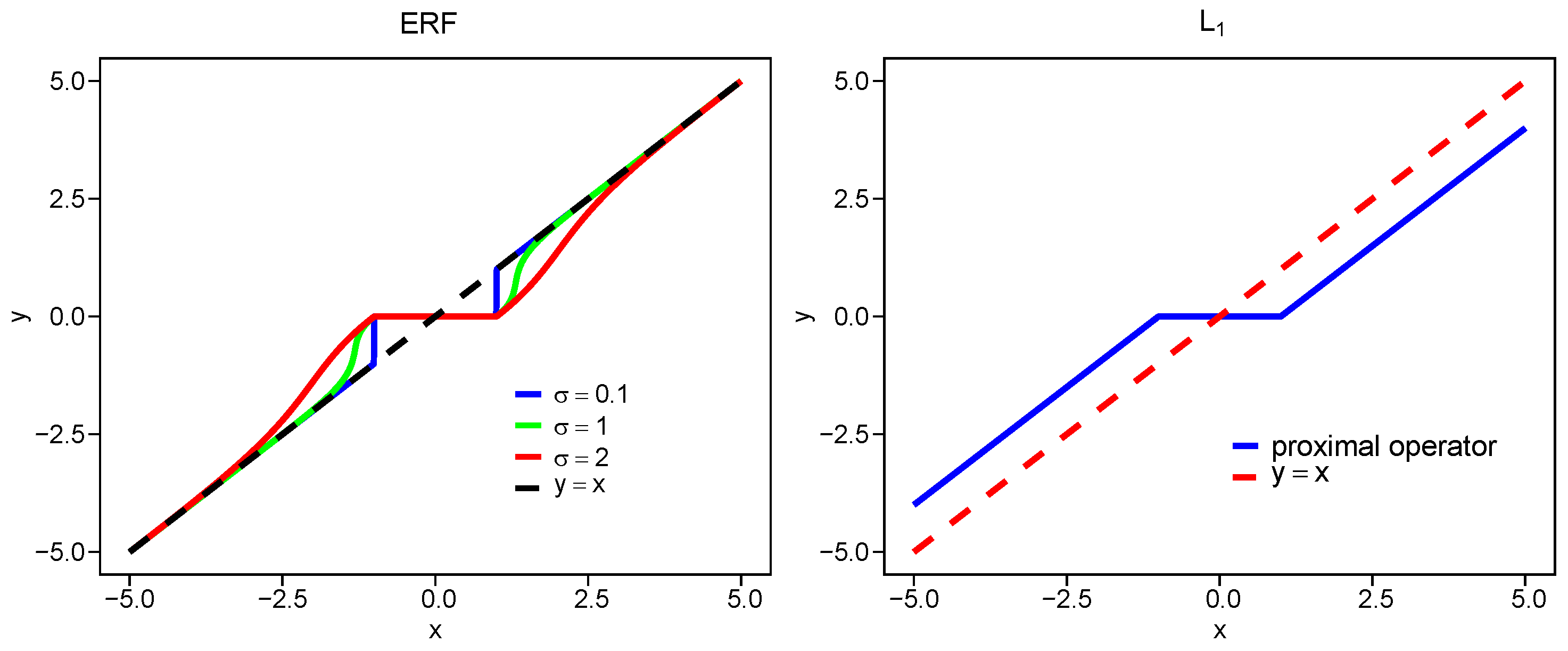
We employ the proximal operator to measure the bias of the penalty function [19]. For a function , the proximal operator of the function f is defined as follows:
In Figure 1, we plot the proximal operators for , , SCAD, and ERF with different at . The proximity of each proximal operator to the line reflects the bias level, that is, a smaller deviation indicates lower bias. The bias of the ERF penalty increases as increases, while for all values , it remains smaller than that of .
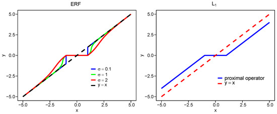
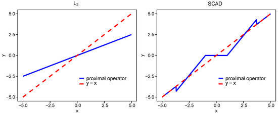
Figure 1.
Common penalized proximal operators.
Considering the non-smoothness of the quantile loss function and the non-convexity of the error function, we can transform Equation (4) into the following form by the iterative reweighted algorithm [17]:
where the corresponding weights are computed by differentiating for each . Specially, we have
We iteratively compute the weights and solve the optimization problem of Equation (9) until convergence is achieved. Gu et al. proposed the proximal ADMM and sparse coordinate descent ADMM algorithms, and proved their global convergence [20]. These two methods are particularly effective for solving high-dimensional sparse quantile regression problems, and show high estimation accuracy and computational efficiency. In this paper, we utilize the IRW-pADMM algorithm, which combines the proximal ADMM algorithm with the iterative reweighted algorithm. Consider the univariate quantile regression method with ERF regularization:
where , is the i-th row of the design matrix , and is the response vector. The IRW-pADMM algorithm is summarized in Algorithm 1. Here, is the soft thresholding operator and we define
where the parameter is the penalty parameter in the augmented Lagrangian of the ADMM algorithm, which affects the convergence speed of the model. is the step size parameter that regulates the update of . Based on the research conducted by Gu et al., is used in the update of to ensure that the matrix in the proximal term
is positive semi-definite, and denotes the largest eigenvalue of the matrix [20].
| Algorithm 1 IRW-pADMM algorithm. | |
| 1: | Input: , , , , , , , maxouter, maxinner |
| 2: | Initialize: , , , |
| 3: | while and do |
| 4: | |
| 5: | , |
| 6: | while and do |
| 7: | |
| 8: | |
| 9: | |
| 10: | |
| 11: | end while |
| 12: | |
| 13: | |
| 14: | end while |
| 15: | return |
We present the two-step DERF-QR Algorithm in Algorithm 2 for the doubly penalized quantile regression method Equation (4). In Algorithm 2, we first initialize the fixed-effect coefficients as , and then compute the initial estimates of the random-effect coefficients using the IRW-pADMM algorithm. Subsequently, we alternately update the fixed- and random-effect coefficients by fixing one set and optimizing the other using the IRW-pADMM algorithm. Specifically, at each iteration k, the fixed-effect coefficients are updated by solving where the response variable is adjusted as . The updated is then substituted into the model to update the random-effects coefficients by solving . The residuals are recalculated as . This alternating optimization procedure is repeated until convergence, which is determined when .
| Algorithm 2 Two-step DERF-QR algorithm. |
|
To proceed further, it is critical to select appropriate penalty parameters. The Schwarz information criterion (SIC) and the generalized approximate cross-validation (GACV) are common selection criteria for quantile regression [21,22,23]. In this paper, we utilize the extended Bayesian information criterion (EBIC) to select penalty parameters [24]:
where , and are the nonzero parameters in the model. p denotes the dimensionality of the variables. The criteria are extended from BIC to EBIC by adding a penalty term to the dimensionality of the variables [24]. The regularization term with parameter , which is imposed on the model by restricting the dimensionality of the variables, improves EBIC in the high-dimensional cases. Specifically, each iteration in the two-step DERF-QR algorithm can be viewed as a univariate penalized quantile regression problem, in which only one parameter is updated at a time. In this paper, we take and in Algorithms 1 and 2.
3. Monte Carlo Simulation
The simulated data are generated from the following model:
Here, let , , , , and . is the covariate vector, and is the correlation between and . For random effects, define for the first three variables, and let , where . denotes the signal-to-noise ratio (SNR). In the following, we introduce PE, TP, and TN to evaluate the variable selection and parameter estimation in the model.
(1) Prediction Error (PE):
where is the estimate of ,
(2) True positives (TP): The number of variables selected correctly.
(3) True negatives (TN): The number of variables excluded correctly.
We show the performance of the DERF-QR method for different correlation coefficients and different sample sizes, that is, there are four scenarios, as follows: (1) , , (2) , , (3) , , (4) , at quantiles , , and , respectively. In addition, we discuss the cases and 2, respectively. Here, and . We select the penalty parameters by EBIC and take . We take the coefficient if , and the same for . Table 1 reports the mean values of PE, standard deviation (SD), and the mean values of TP and TN based on 100 replications.

Table 1.
PE, TP, and TN for different correlation coefficients and sample sizes.
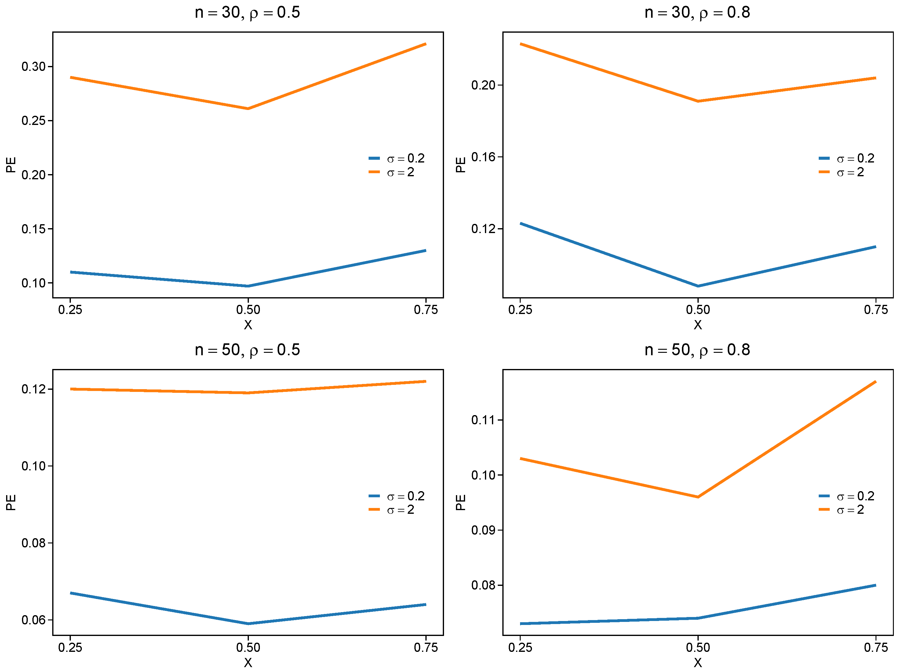
The simulation shows that we could select the right variable by DERF-QR in all experimental conditions in Table 1. Also, PE decreases and TN decreases slightly when sample size n increases. It is observed that stronger correlation yields smaller PE values, compared with . The DERF-QR method in strong-correlation scenarios shows robust performance due to its adaptive penalty weights. This improves coefficient estimation accuracy under strong variable correlations. Parameter significantly influences the result. The PE value of is greater than that of . Additionally, we observe that the model is less sensitive to variations of the parameter at the median quantile. The median quantile regression also yields a smaller PE value, compared with other quantiles. The simulation results are presented in Figure 2.
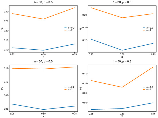
Figure 2.
PE for different correlation coefficients and sample size.
Consider different SNR and , and define three different random-effect matrices, and , to investigate the effects of different SNRs and random effects on the model. Take , and . Table 2 indicates the average values of PE, TP, and TN in 100 simulations.
Table 2.
Average values of PE, TP, and TN in different conditions.
In Table 2, as the SNR becomes greater and the influence of random effects increases, PE and SD increase gradually, while TN decreases slightly. If the SNR becomes greater, the model is less accurate and loses stability. In this case, it is more likely to select incorrect variables. However, we observe that even in the case and , there are still relatively low errors for the model, and most incorrect variables are excluded. In general, an increase in SNR and random effects significantly impacts the coefficient estimation and variable selection. Meanwhile, the model is robust and effective in the process.
To investigate the performance of DERF-QR and other methods, we discuss the following four scenarios with different error distributions. and which denotes
We would make comparisons among the following four methods: Quantile Regression without penalization (QR), Doubly penalized Lasso regularized Quantile Regression (DLQR), Doubly penalized SCAD regularized Quantile Regression (DSQR), and the DERF-QR model with the parameter proposed in this paper. Consider two distinct scenarios as follows:
Repeat 100 times, and take , and . Table 3 and Table 4 depict the results, and Figure 3 and Figure 4 show the boxplots of PE for these two models.
Table 3.
Comparison among different methods in the sparse model.
Table 4.
Comparison among different methods in the dense model.
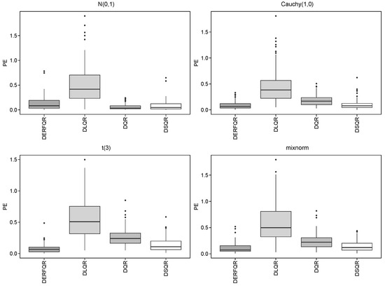
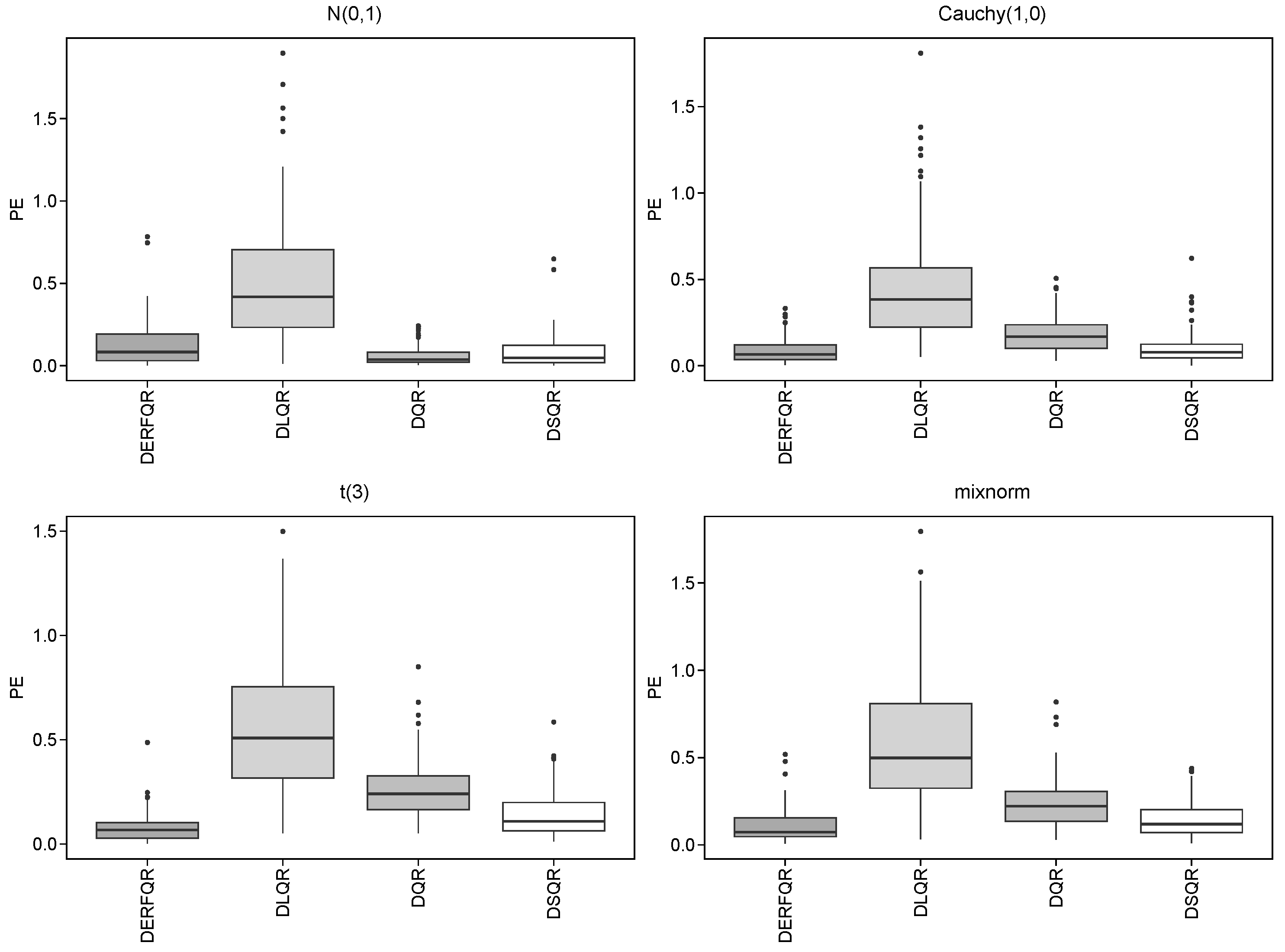
Figure 3.
Boxplots of different methods in the sparse model.
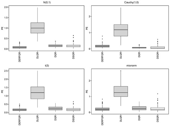
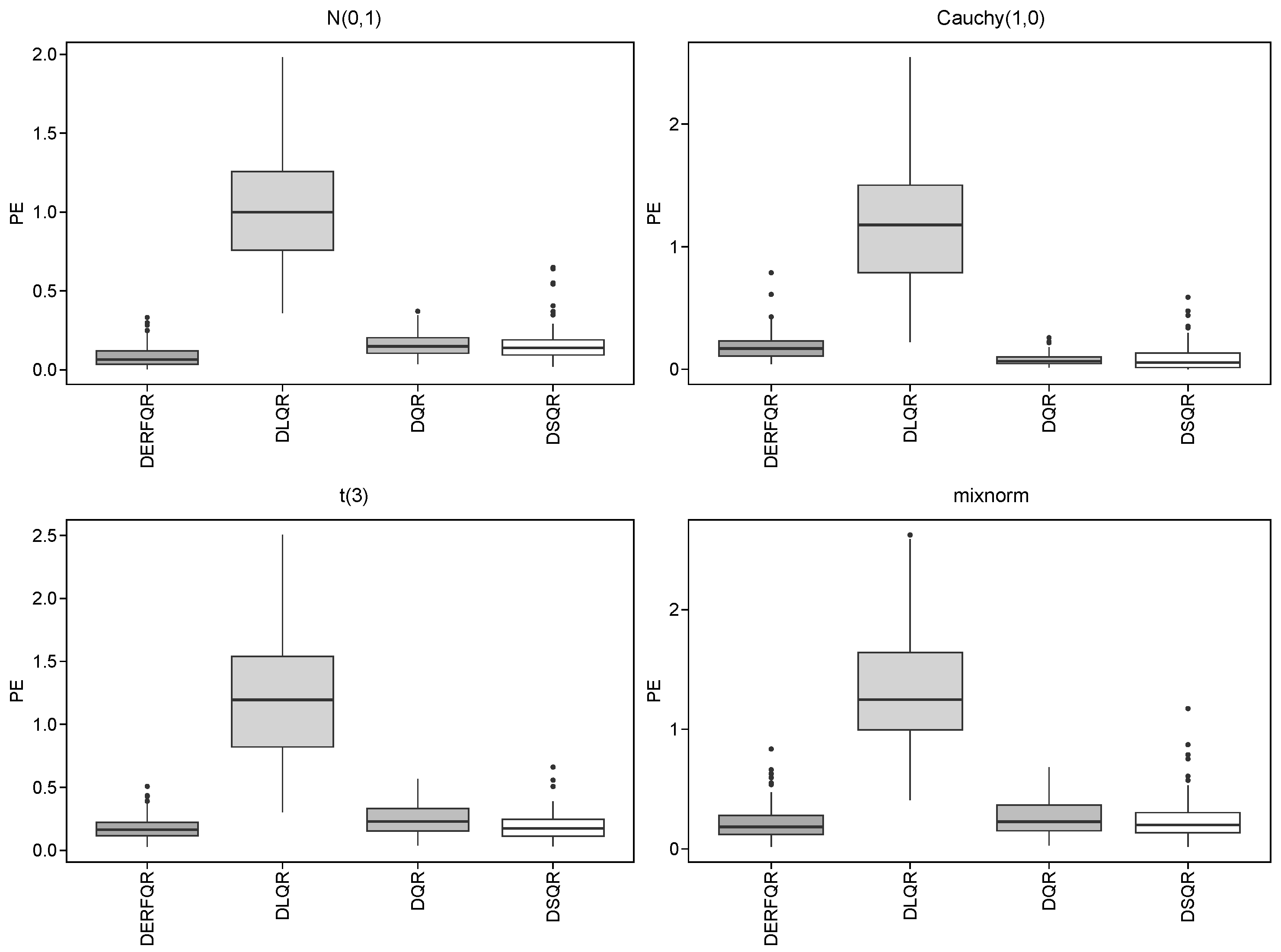
Figure 4.
Boxplots of different methods in the dense model.
It can be observed from Table 3 that we could select the right variables and derive lower PE by using DLQR, DSQR, and DERF-QR in the sparse model. The DERF-QR method shows robust coefficient estimation performance. Notably, it excludes up to 80% of incorrect variables across all cases. There are four different error distributions in Table 3, where there are a significant number of outliers in the Cauchy distribution with heavy tails. DERF-QR exhibits relatively greater PE in the Cauchy distribution but maintains the lowest PE among all methods across other distributions. It is unstable to exclude incorrect variables by DSQR, even though DSQR performs well in coefficient estimation and its PE is close to that of DERF-QR. The PE in DLQR is relatively greater, even though it could exclude incorrect variables clearly. Generally, DERF-QR is the optimal one of these four methods.
In the dense model, DERF-QR still performs the best among the four methods. We could select the correct variables from all by these four methods. In most cases, the Cauchy distribution shows smaller errors, while the mixnorm distribution results in relatively greater errors. For Cauchy distribution, we obtain lower PE by DQR and DSQR, compared with DERF-QR. In other distributions, the PE of DSQR is similar to that of DERF-QR. The PE of DLQR is slightly greater than the others in all cases.
4. Financial Data Analysis
The DERF-QR method is developed in the financial statements and balance sheets of 12 companies from 2009 to 2023 [25]. Due to missing data, we select 10 companies from 2009 to 2022 for simulation. The revenue is regarded as the response variable. We aim to find the factors influencing the revenue. Consider 20 variables as explanatory variables as in Table 5.
Table 5.
Explanatory variables.
In Table 5, X20, X21, X22, X23, X24, and X25 denote the numerical variables for the company’s six categories. Specifically, each category is represented using binary indicators, where applicable categories are marked with a 1 and non-applicable ones with a 0. The other explanatory variables are continuous. Consider the following linear mixed-effects model:
where denotes the revenue of company i in year j. For the random-effects coefficients , we consider that random effects exist in all variables, i.e.,
We empirically evaluated DERF-QR under and , at quantile levels , , and . For comparison, we also included the DLQR method. The mean squared error (MSE) is defined as
and the number of non-zero coefficients (model size, MS) is used to assess variable selection performance.
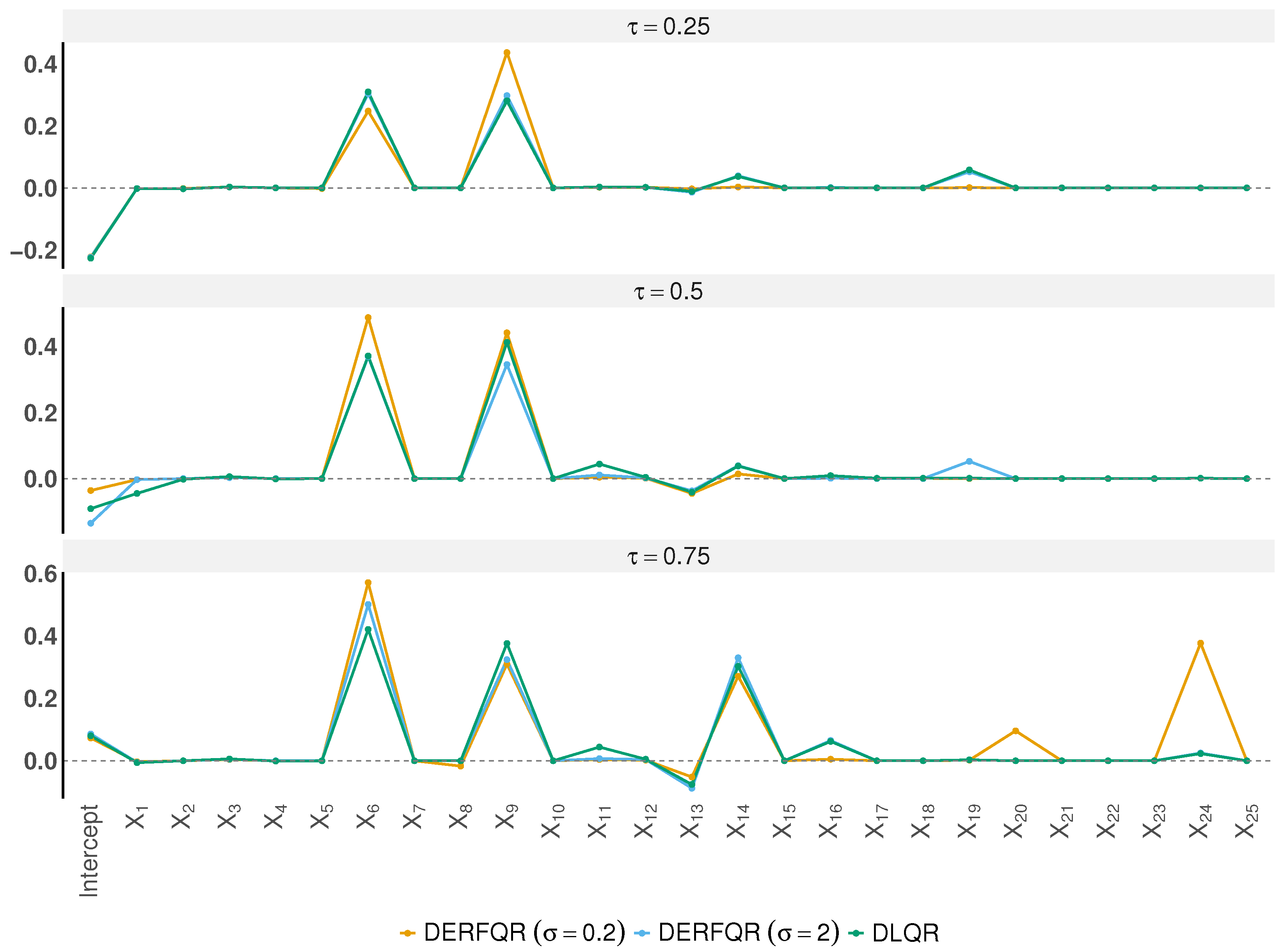
Figure 5 presents the estimated coefficients across quantiles. Both DERF-QR and DLQR successfully eliminate most irrelevant variables. Notably, all methods consistently selected X6 and X9, while the other variables are very small or shrink to zero. This indicates that gross profit and EBITDA have a significant impact on revenue. We find that variable selection differs across quantile levels. At , all three methods tend to select X6, X9, and X14.

Figure 5.
Coefficient estimation results across different quantile levels.
Table 6 shows the MSE and MS for each method. When , DERF-QR achieves the lowest MSE at and . With , DERF-QR attains the lowest MSE at and also yields the smallest MS at both and . DERF-QR consistently yields the lowest MSE across quantile levels. Overall, DERF-QR consistently achieves superior estimation accuracy and variable selection across quantile levels.
Table 6.
MSE and MS for different methods at various quantile levels.
5. Discussion
We conducted Monte Carlo simulations of the proposed method under various conditions, including different SNRs, sample sizes n, correlation coefficients , and sparsity levels. The results demonstrate that DERF-QR consistently achieves the lowest PE and highest TN in most scenarios, indicating its strong performance in both variable selection and parameter estimation.
Despite DERF-QR’s strong overall performance, its estimation accuracy declines under Cauchy-distributed errors. This can be attributed to the heavy-tailed nature of the Cauchy distribution, which introduces more extreme outliers and may compromise the robustness of coefficient estimation. Therefore, evaluating the robustness of DERF-QR and related methods under heavy-tailed error distributions remains an important direction for future research.
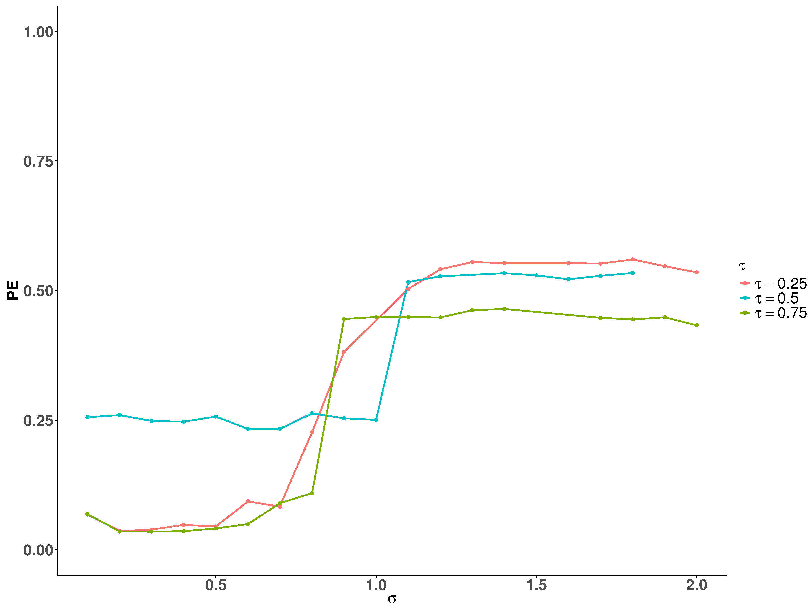
The simulation results show that significantly affects DERF-QR’s estimation performance. We conducted simulations under the setting to examine how different values of affect the PE at , , and , respectively. Taking , , , Figure 6 shows the trend of how the PE varies with increasing at different quantile levels. As increases, the PE increases across all three quantile levels. When , the impact of on PE is relatively smaller compared to the other quantiles. Based on these observations, we recommend selecting the within a relatively small range through cross-validation in practical applications.
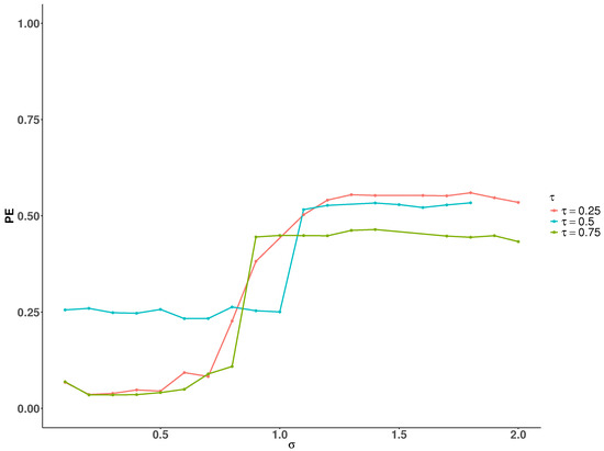
Figure 6.
Correlation coefficients and sample size.
Additionally, we focus exclusively on EBIC performance for and selection. Other parameter selection approaches, including the Schwarz information criterion (SIC), generalized approximate cross-validation (GACV), and cross-validation methods, were not evaluated in our comparative analysis. Future comparisons of these methods would strengthen tuning strategy evaluation.
6. Conclusions
In this paper, we established the DERF-QR method for both parameter estimation and variable selection in the linear mixed-effects model. We studied a non-convex and smooth error function regularization, which is quite different from traditional regularization methods for variable selection in quantile regression for this model. We derived the asymptotic behavior of the penalty, and viewed the penalty as a close approximation to regularization as .
We conducted simulations under various scenarios. DERF-QR yielded lower PE across various signal-to-noise ratios and random-effect structures. Even under the challenging setting of and , it retained low PE and successfully eliminated 80% irrelevant variables. When and , PE remained lower than under and , indicating strong stability in the presence of larger sample sizes and high correlation. Compared with other penalized quantile regression methods, DERF-QR consistently achieved the lowest PE and the highest TN in both sparse and dense settings, demonstrating robust performance in coefficient estimation and variable selection. We also developed this method for financial data and showed that it is practically effective.
Our proposed DERF-QR method effectively extends penalized quantile regression for linear mixed-effects models, demonstrating excellent performance in both parameter estimation and variable selection. There are still some open issues for future research in this field. For instance, the IRW-pADMM algorithm involves parameter selection, and selecting inappropriate parameters could result in slow convergence during the iteration process. Therefore, improving the efficiency of the algorithm remains an important topic for future work. Additionally, this approach can be further applied and studied in other models, such as spatial mixed-effects models or generalized linear mixed models.
Author Contributions
Methodology, Z.H.; Writing—original draft, Z.H.; Writing—review & editing, X.H.; Project administration, X.H. All authors have read and agreed to the published version of the manuscript.
Funding
This research was funded by [Double First Class Special Project, Jiangsu, China] grant number [1014/B22017010224] And The APC was funded by [Hohai University].
Institutional Review Board Statement
Not applicable.
Data Availability Statement
The original contributions presented in the study are included in the article, further inquiries can be directed to the corresponding author.
Conflicts of Interest
The authors declare no conflict of interest.
References
- Khan, I.; Muhammad, I.; Sharif, A.; Khan, I.; Ji, X. Unlocking the potential of renewable energy and natural resources for sustainable economic growth and carbon neutrality: A novel panel quantile regression approach. Renew. Energy 2024, 221, 119779. [Google Scholar] [CrossRef]
- Qu, L.; Hao, M.; Sun, L. Sparse composite quantile regression with ultrahigh-dimensional heterogeneous data. Stat. Sin. 2022, 32, 459–475. [Google Scholar]
- Cheng, C.; Feng, X.; Huang, J.; Liu, X. Regularized projection score estimation of treatment effects in high-dimensional quantile regression. Stat. Sin. 2022, 32, 23–41. [Google Scholar] [CrossRef]
- Tan, K.M.; Wang, L.; Zhou, W.X. High-dimensional quantile regression: Convolution smoothing and concave regularization. J. R. Stat. Soc. Ser. B Stat. Methodol. 2022, 84, 205–233. [Google Scholar] [CrossRef]
- Wang, M.; Zhang, X.; Wan, A.T.; You, K.; Zou, G. Jackknife model averaging for high-dimensional quantile regression. Biometrics 2023, 79, 178–189. [Google Scholar] [CrossRef]
- Powell, D. Quantile regression with nonadditive fixed effects. Empir. Econ. 2022, 63, 2675–2691. [Google Scholar] [CrossRef]
- Belloni, A.; Chen, M.; Madrid Padilla, O.H.; Wang, Z. High-dimensional latent panel quantile regression with an application to asset pricing. Ann. Stat. 2023, 51, 96–121. [Google Scholar] [CrossRef]
- Koenker, R.; Bassett, G., Jr. Regression quantiles. Econom. J. Econom. Soc. 1978, 46, 33–50. [Google Scholar] [CrossRef]
- Lamarche, C. Quantile regression for panel data and factor models. In Oxford Research Encyclopedia of Economics and Finance; Oxford University Press: Oxford, UK, 2021. [Google Scholar]
- Tibshirani, R. Regression shrinkage and selection via the lasso. J. R. Stat. Soc. Ser. B Stat. Methodol. 1996, 58, 267–288. [Google Scholar] [CrossRef]
- Fan, J.; Li, R. Variable selection via nonconcave penalized likelihood and its oracle properties. J. Am. Stat. Assoc. 2001, 96, 1348–1360. [Google Scholar] [CrossRef]
- Koenker, R. Quantile regression for longitudinal data. J. Multivar. Anal. 2004, 91, 74–89. [Google Scholar] [CrossRef]
- Li, H.; Liu, Y.; Luo, Y. Double penalized quantile regression for the linear mixed effects model. J. Syst. Sci. Complex. 2020, 33, 2080–2102. [Google Scholar] [CrossRef]
- Bondell, H.D.; Krishna, A.; Ghosh, S.K. Joint variable selection for fixed and random effects in linear mixed-effects models. Biometrics 2010, 66, 1069–1077. [Google Scholar] [CrossRef] [PubMed]
- Qi, X.; Xu, X.; Feng, Z.; Peng, H. Component selection and variable selection for mixture regression models. Comput. Stat. Data Anal. 2025, 206, 108124. [Google Scholar] [CrossRef]
- Guo, W.; Lou, Y.; Qin, J.; Yan, M. A novel regularization based on the error function for sparse recovery. J. Sci. Comput. 2021, 87, 31. [Google Scholar] [CrossRef]
- Candes, E.J.; Wakin, M.B.; Boyd, S.P. Enhancing sparsity by reweighted ℓ1 minimization. J. Fourier Anal. Appl. 2008, 14, 877–905. [Google Scholar] [CrossRef]
- Zhang, C.H. Nearly unbiased variable selection under minimax concave penalty. Ann. Stat. 2010, 38, 894–942. [Google Scholar] [CrossRef]
- Boyd, S.; Parikh, N.; Chu, E.; Peleato, B.; Eckstein, J. Distributed optimization and statistical learning via the alternating direction method of multipliers. Found. Trends® Mach. Learn. 2011, 3, 1–122. [Google Scholar]
- Gu, Y.; Fan, J.; Kong, L.; Ma, S.; Zou, H. ADMM for high-dimensional sparse penalized quantile regression. Technometrics 2018, 60, 319–331. [Google Scholar] [CrossRef]
- Schwarz, G. Estimating the dimension of a model. Ann. Stat. 1978, 6, 461–464. [Google Scholar] [CrossRef]
- Yuan, M. GACV for quantile smoothing splines. Comput. Stat. Data Anal. 2006, 50, 813–829. [Google Scholar] [CrossRef]
- Koenker, R.; Ng, P.; Portnoy, S. Quantile smoothing splines. Biometrika 1994, 81, 673–680. [Google Scholar] [CrossRef]
- Chen, J.; Chen, Z. Extended Bayesian information criteria for model selection with large model spaces. Biometrika 2008, 95, 759–771. [Google Scholar] [CrossRef]
- R. Rish59, Financial Statements of Major Companies (2009–2023), Kaggle. 2023. Available online: https://www.kaggle.com/datasets/rish59/financial-statements-of-major-companies2009-2023 (accessed on 27 May 2025).

Disclaimer/Publisher’s Note: The statements, opinions and data contained in all publications are solely those of the individual author(s) and contributor(s) and not of MDPI and/or the editor(s). MDPI and/or the editor(s) disclaim responsibility for any injury to people or property resulting from any ideas, methods, instructions or products referred to in the content. |
© 2025 by the authors. Licensee MDPI, Basel, Switzerland. This article is an open access article distributed under the terms and conditions of the Creative Commons Attribution (CC BY) license (https://creativecommons.org/licenses/by/4.0/).