Ensemble Learning-Based Weed Detection from a Duck’s Perspective Using an Aquatic Drone in Rice Paddies ^†

Abstract

Semantic segmentation using neural networks (NNs) has significant potential for weed detection in agricultural fields. However, conventional datasets captured from aerial perspectives often fail to detect weeds that are either hidden beneath crops or submerged in water. This study proposes a method for accurately detecting weed pixels through ensemble learning-based semantic segmentation, using forward-facing images captured by a camera mounted on an aquatic drone navigating between rice plants. We also present a paddy field weed image dataset constructed to train the NN models. Multiple semantic segmentation models were trained, compared, and evaluated, achieving a weed intersection over union (IoU) of 0.441, mean IoU (mIoU) of 0.706, and pixel accuracy of 0.971.

1. Introduction

In recent years, efforts related to sustainable development goals and movements emphasizing environmental sustainability have increased. The field of agriculture is no exception, with a growing global momentum toward organic farming. In Japan, the Ministry of Agriculture, Forestry, and Fisheries formulated the “Strategy for Sustainable Food Systems, MeaDRI” in 2021, aiming to enhance the productivity and sustainability of the food, agriculture, forestry, and fishery sectors through innovation [1]. One of the key goals of this strategy is to expand the area under organic farming from approximately 27,000 ha in 2021 to 1,000,000 ha by 2050. The Act on Promotion of Organic Agriculture defines organic farming as an agricultural practice that meets the specific conditions established under this law:

• Do not use chemically synthesized fertilizers or pesticides;
• Do not employ genetically modified technologies;
• Employ agricultural production methods that minimize the environmental impacts of agricultural activities to the maximum extent.

However, the area under organic farming in Japan has increased by approximately 7000 ha over the ten-year period since 2011. According to a survey on awareness and intentions regarding organic farming conducted among organic producers [2], a significant proportion of respondents cited labor and time requirements in production as major reasons for maintaining the current cultivation area or even reducing it, rather than expanding it. Weed control is one of the main factors contributing to the perception that organic farming is more labor-intensive than conventional farming. Physical weed removal, whether by hand or using machinery, is generally more time-consuming and labor-intensive than the use of herbicides in conventional farming.

In response to broader challenges in the agricultural sector, such as declining and aging farming populations, smart agriculture, which integrates advanced technologies with traditional farming practices, has been gaining attention [3]. Advancements in information technology, robotics, and artificial intelligence (AI) have enabled the application of information communication technology and robotic systems from various perspectives.

The Aigamo Robot [4], for instance, is an autonomous weeding robot designed for rice paddies. It stirs the paddy soil with a spiral screw, thereby muddying the water and suppressing weed growth. Additionally, various technologies have been implemented, including greenhouse environmental control systems [5] and autonomous driving combines [6].

Weed control is a primary challenge in the implementation of organic farming in paddy fields. Nile-JZ [7] is a drone capable of autonomous flight and automated pesticide spraying. It can sense crops using an onboard camera and control weeds through pesticide application. However, certain limitations exist to the use of drone-based smart farming technologies for weed management in paddy fields. Because of their top-down imaging nature, drones often struggle to capture weeds that are overlapped by crops or are submerged in water. When weeds are missed during detection, pesticide application becomes ineffective and potentially hinders crop growth. As weeds may be concealed beneath the canopy from an aerial viewpoint, it is necessary to capture field information from alternative camera angles. Moreover, drones rely on pesticide-based weed control, which is incompatible with the principles of organic farming, where the use of chemical pesticides is strictly prohibited. Therefore, weed control must be performed using physical removal methods in organic systems. However, aerial drones are not suitable for non-chemical weed management, because they are incapable of physically removing weeds. An aquatic drone, a small vessel capable of navigating water, has the potential to address these challenges. By equipping the aquatic drone with a camera, it is possible to capture images of the paddy field from a lower near-horizontal angle, closer to the crops and weeds, compared with aerial drones. This imaging perspective allows for the detection of weeds that may be missed in top-down views, such as those hidden beneath the crop canopy or submerged in water. Furthermore, an aquatic drone equipped with a mechanical weeding system can perform physical weed control. This approach aligns with the principles of organic farming and offers a non-chemical method of weed management that aerial drones cannot perform.

To promote the development of organic farming, it is essential to reduce the labor and effort required for its implementation. Weed management is a key challenge in organic farming. Identifying the precise locations of weeds using AI can lead to more efficient weeding and help alleviate the labor intensity associated with weed control. However, as will be elaborated in detail in Section 2, current weed detection algorithms primarily rely on aerial photography, a method that proves ineffective in reducing labor in organic farming. This study aimed to comprehensively identify weed-infested areas in paddy fields. To this end, we propose a method for detecting weed pixels using ensemble learning-based neural networks (NNs) for semantic segmentation, applied to forward-facing paddy field images captured by a camera mounted on an aquatic drone. Additionally, we constructed a paddy field weed image dataset to train the NN models. The dataset comprised images captured from an aquatic drone and corresponding binary mask images labeled as either weed or background. By analyzing paddy field conditions from a unique low-angle, near-horizontal viewpoint, achieved from a floating aquatic platform, we anticipate that this method will enable the accurate and exhaustive detection of weed presence in paddy fields, which is difficult to accomplish using conventional top-down imaging.

This paper is an extended version of the conference paper presented at the IEEE Global Conference on Consumer Electronics (GCCE), Kitakyushu, Japan, October 2024, titled “Weed Detection from the Duck’s Perspective Using Aqua-Drone in Rice Paddies”. In this extended version, we have applied ensemble learning to improve segmentation accuracy. Additional experiments and analysis have also been included.

2. Related Works

2.1. Deep Learning-Based Image Recognition

2.1.1. Semantic Segmentation

Image recognition is a key task in machine learning (ML). Supervised learning is commonly used in deep learning (DL)-based image recognition, in which an NN model is trained using a dataset comprising input images and corresponding ground truth (GT) labels. Among various image recognition techniques, semantic segmentation is notable for its ability to identify objects at the pixel level within an image. Compared with other methods such as image classification and object detection, semantic segmentation provides more detailed spatial information about the content of an image [8,9].

2.1.2. Transfer Learning

The training of NNs typically requires large amounts of data. However, collecting such extensive datasets often requires considerable time and effort. Transfer learning is typically employed to address this issue. Transfer learning is a technique in which the parameters of a NN trained on a dataset that is different from the target task are used as the initial values for training. This approach has been shown to be effective in improving performance and reducing training time. Because training on the non-target dataset is performed prior to the target task, this process is referred to as pretraining. A widely used dataset for pretraining is ImageNet [10], which contains over 14 million images and more than 20,000 label categories, and is freely accessible to researchers. PyTorch 2.6.0 [11], an open-source ML library for Python 3.11, provides various pretrained models based on ImageNet, allowing users to easily leverage transfer learning in their applications.

2.1.3. Ensemble Learning

Ensemble learning is an ML technique that combines multiple models to achieve a higher predictive accuracy and better generalization performance [12]. Three primary types of ensemble learning methods exist:

• Bagging (bootstrap aggregation): This method involves random division of a dataset and independent training of multiple models. The final prediction is obtained by averaging the model outputs.
• Boosting: Models are trained sequentially, with each new model focusing on correcting errors made by previous models.
• Stacking: This approach combines the outputs of multiple models by feeding them into a metamodel that learns how to integrate their predictions best.

2.2. Weed Segmentation

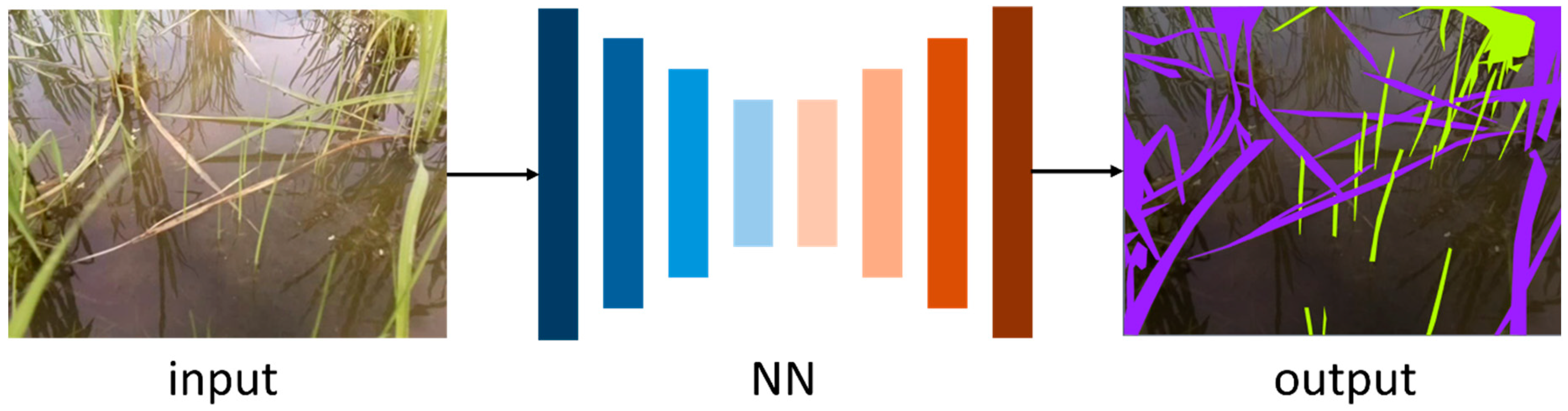
Research on weed detection has been conducted in recent years [13,14,15,16,17]. Most of these studies use UAVs to obtain data. Zou et al. developed a dataset based on aerial images captured from corn, wheat, and soybean fields and applied semantic segmentation to detect weeds, achieving an intersection over union (IoU) of 0.9291 [13]. Ma et al. constructed a dataset using aerial images of paddy fields and performed three-class semantic segmentation to classify weeds, rice plants, and the background, with a mean IoU (mIoU) of 0.618 [14]. The dataset used in their study is publicly available and can be used for further research. Building on this, Yang et al. performed training and inference using multiple NN models on the same dataset and achieved a higher mIoU of 0.781 with their proposed MSFCA-Net [17]. In addition to the paddy field dataset, their experiments included the soybean, sugar beet, and carrot datasets. The paddy field dataset yielded the lowest segmentation accuracy, suggesting that weed detection in paddy fields is particularly challenging. As described above, numerous studies have reported semantic segmentation for weed detection. However, most of these studies have utilized datasets based on aerial imagery. As discussed in Section 1, these approaches do not resolve the issue of weeds being hidden beneath rice plants and not being visible in the captured images in the first place. To address this limitation, we proposed an alternative imaging approach using an aquatic drone equipped with a forward-facing camera to achieve an mIoU of 0.676 [18].

3. Method

3.1. Dataset

To train an NN for weed detection, a dataset comprising input images and corresponding GT mask images is required. For semantic segmentation, creating GT masks involves a process known as annotation, in which each pixel of the input image is labeled according to its class [19]. In this study, input image data were collected in the form of MP4 videos. Individual frames were extracted and saved as JPEG images, which were thereafter used to create binary GT mask images in PNG format, labeling each pixel as either “weed” or “background”. Therefore, a custom dataset was constructed for weed detection.

3.2. Neural Network

In this study, we employed a convolutional neural network (CNN) architecture tailored for semantic segmentation to perform pixel-level weed detection in rice field images. The model adopts an encoder–decoder structure and was selected based on its demonstrated performance in previous segmentation tasks, as well as its availability as a pre-trained architecture suitable for fine-tuning through transfer learning techniques. Inference by the network is performed as shown in Figure 1.

3.2.1. UNet++

UNet++ is an improved version of the original UNet architecture [20] initially developed for medical image segmentation. The UNet architecture comprises an encoder–decoder structure with skip connections that link the encoder outputs at each level to the corresponding decoder layers. These skip connections help preserve the spatial information that is otherwise lost during downsampling in the encoder, enabling accurate region extraction. UNet++ enhanced this structure by embedding a series of nested UNets between the encoder and decoder paths. This nested architecture enables more effective transmission of features from the encoder to the decoder, thereby improving segmentation performance. The additional intermediate layers allow for better feature refinement, leading to more precise delineation of the object boundaries compared with the original UNet.

3.2.2. DeepLabV3+

DeepLabV3+ is a semantic segmentation model based on an encoder–decoder architecture and is an improved version of DeepLabV3 [21]. In DeepLabV3, a key component is the use of atrous (dilated) convolution, an operation that extends the standard convolution by introducing gaps between kernel elements, allowing the network to capture multiscale contextual information without increasing the computational cost. The atrous convolution is defined as follows:

$$y_i=\sum _k{x}_{i+rk}{w}_k,$$

(1)

where y denotes the output feature map, x denotes the input, w denotes the filter weight, i and k denote the positions in the feature map and filter, respectively, and r denotes the dilation rate that determines the spacing between the kernel elements. DeepLabV3+ extends DeepLabV3 by incorporating a decoder module with skip connections. In this design, the features extracted by the encoder are upsampled by a factor of four and fused with low-level features from earlier layers. This combination allows for more precise boundary delineation and improved segmentation accuracy compared with DeepLabV3.

3.3. Training Method

The model described in Section 3.2 is trained using the dataset presented in Section 3.1. In this section, the various conditions and settings used during the training process are described.

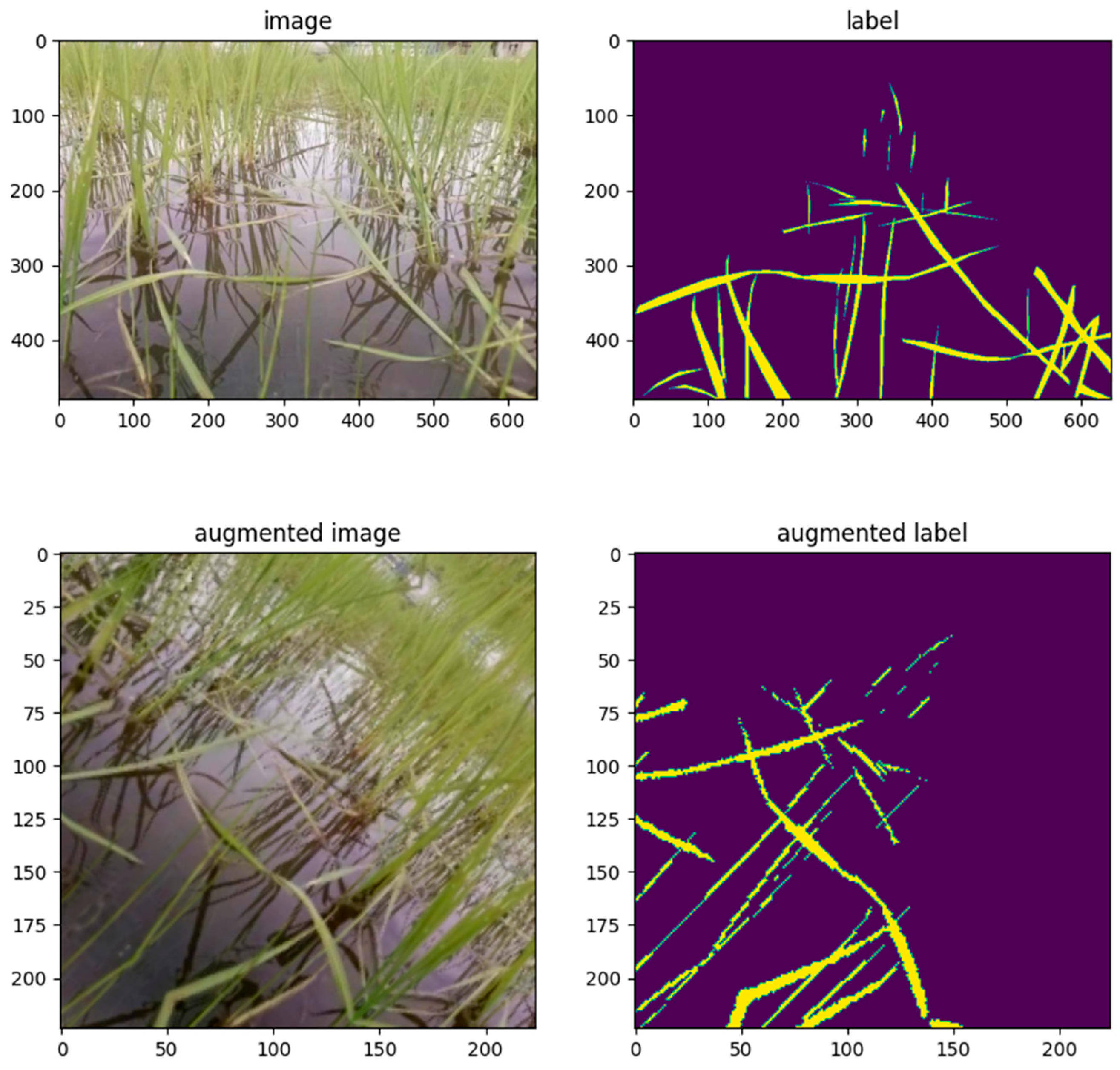
3.3.1. Data Augmentation

In scenarios in which the dataset is limited in size, data augmentation is commonly employed to enhance the diversity of the training samples and improve the robustness of the model during inference [22]. The following augmentation techniques were applied: horizontal flipping, translation, scaling, rotation, brightness, and contrast adjustments.

3.3.2. Loss Function

When training NNs, it is essential to evaluate the difference between the network’s predictions and GT masks, referred to as the loss, and optimize the network parameters such that this loss is minimized [23]. A loss function is a mathematical formulation used to quantify this difference, and various loss functions have been designed to suit different learning objectives. In this study, the dataset exhibited class imbalance, with a significant disparity between the number of weed pixels and background pixels. To address this issue, we adopt Dice Loss (Equation (2)), which is specifically designed to facilitate the effective learning of imbalanced data.

$$\mathrm{D}\mathrm{i}\mathrm{c}\mathrm{e}\mathrm{L}\mathrm{o}\mathrm{s}\mathrm{s}=1-{\displaystyle \frac{2{\sum }_{1\le w\le W}{\sum }_{1\le h\le H}{t}_{w,h}{p}_{w,h}}{{\sum }_{1\le w\le W}{\sum }_{1\le h\le H}(t_{w,h}+p_{w,h})}}$$

(2)

Here, W and H denote the width and height of the image, respectively. The variable t_{w,h} represents the GT mask, where 1 indicates a weed pixel and 0 indicates a background pixel, and p_{w,h} denotes the predicted mask with the same pixel-wise labeling.

3.3.3. Optimizer

In the NN training, the loss computed in the previous section is used to iteratively update the network parameters to minimize the loss. The optimizer is the algorithm responsible for parameter optimization. In this study, we employed the Adam optimizer [24], which is defined in Equations (3)–(5):

$$m_{t,i}={\beta }_1{m}_{t-1,i}+\left(1-{\beta }_1\right)g_{t,i}$$

(3)

$$v_{t,i}={\beta }_2{v}_{t-1,i}+\left(1-{\beta }_2\right)g_{t,i}^2$$

(4)

$$\mathsf{\Delta }{w}_{t,i}=-{\displaystyle \frac{ϵ}{\sqrt{v_{t,i}}}}{m}_{t,i}$$

(5)

Adam is an optimization algorithm that combines the advantages of two previous methods: AdaGrad and RMSProp. It is widely used in NN training because of its efficiency and stability. Here, g_{t,i} denotes the gradient of the loss function, m_{t,i} represents the exponential moving average of the gradients, and v_{t,i} represents the exponential moving average of the squared gradients. The term $\mathsf{\Delta }$ w_{t,i} indicates the update applied to the network parameter. The subscript refers to the current time step, and i denotes the index of the parameter being optimized. The symbols $\beta$ and $ϵ$ are hyperparameters that control the behavior of the optimizer.

3.3.4. Early Stopping

When a model performs well on training data but fails to generalize to unseen data such as validation or test datasets, this phenomenon is referred to as overfitting. It is essential to take precautions against overfitting during the training of NNs. In general, as training progresses, errors in the validation and test datasets tends to stop decreasing, indicating the onset or progression of overfitting. Overfitting reduces the generalization capability of the model and negatively affects its performance during inference. To address this issue, a technique known as early stopping is often employed, in which training is terminated when loss of the validation dataset ceases [25]. In this study, training was halted if no improvement in validation loss was observed over 100 consecutive epochs. The model exhibiting the lowest validation loss was selected as the final trained model and subsequently evaluated using the test dataset.

3.4. Bagging

To improve inference accuracy, ensemble learning was incorporated in this study. Among the various ensemble learning methods, we adopted bagging (bootstrap aggregation). Bagging involves independently training multiple weak learners and aggregating their prediction results, typically by averaging or summation. This approach enables individual models to complement each other, thereby enhancing the overall robustness and accuracy of the predictions. Consequently, bagging is expected to yield more generalized and reliable inference performance [26].

4. Experimentation

This section describes the experimental methodology for the proposed approach outlined in Section 3. Unless otherwise specified, all codes were implemented using PyTorch.

4.1. Making Dataset

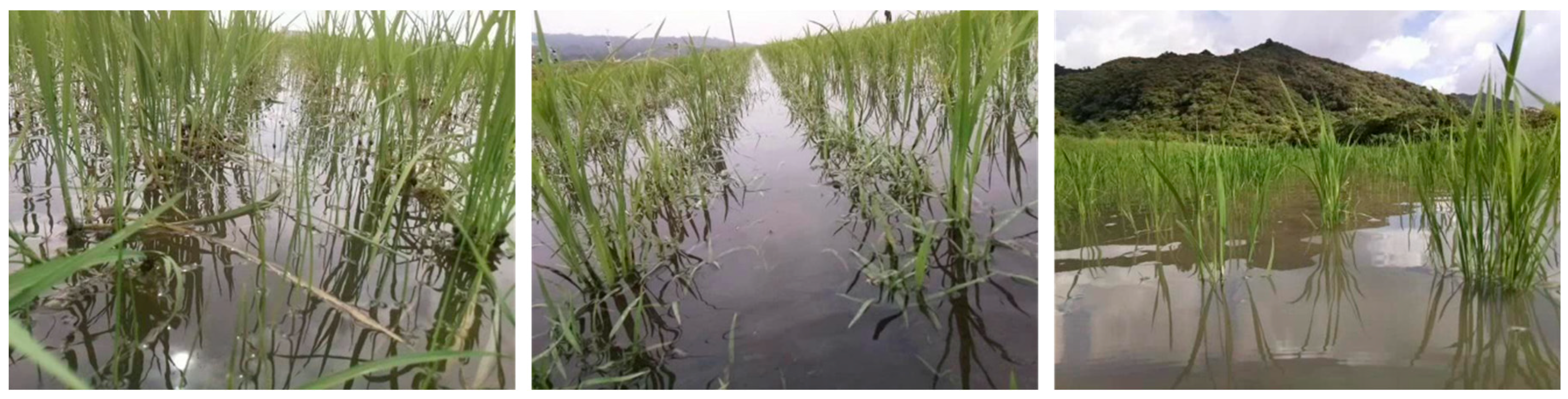
4.1.1. Data Collection

For dataset construction, we acquired videos in MP4 format using a Raspberry Pi Camera V2 (Raspberry Pi Foundation, Cambridge, UK) mounted on a boat designed to simulate an aquatic drone that was 15 cm in width, 30 cm in length, and 17.5 cm in height (Figure 2). The camera was controlled using Raspberry Pi 4 and mounted in front of the boat at a downward angle of 30°. The video resolution was set to 640 × 480 pixels, with a frame rate of 30 fps. During data collection, the boat was manually pushed from behind to navigate between rows of rice plants. The videos were recorded in paddy fields located in Niigata Prefecture, Fukushima Prefecture, and Iriomote Island, Japan. These three fields exhibit different environmental conditions, and incorporating images from each location into the dataset contributes to its overall diversity. Figure 3 presents representative examples of images captured at each site. In the Niigata field, weeds tend to grow vertically with elongated stems. In the Fukushima field, low-height weeds are frequently observed around the rice plants. In contrast, the field on Iriomote Island showed a tendency toward sparse weed presence.

4.1.2. Annotation

Annotations were made using Roboflow [27], a platform for developing AI models. Roboflow provides an intuitive interface that supports annotation, data augmentation, model training, and other DL-related tasks. However, in the present study, it was used solely for annotation. The binary GT masks, comprising weeds and background labels, were created as follows:

Conversion from Video to Images. Video files in MP4 format were converted into JPEG images using OpenCV, a Python library for computer vision.

Image Selection. From the extracted JPEG images, frames to be included in the dataset were selected. Pseudorandom numbers were generated in Python to randomly sample the images, which were subsequently uploaded to the Roboflow annotation tool.

Weed Pixel Annotation. Annotation of weed pixels was performed using the **Polygon Tool** provided by Roboflow. Annotators were manually clicked along the contours of the weeds using a mouse, and the interior region was automatically labeled as a weed pixel. Figure 4 shows an example annotation, where the pixels highlighted in light green represent the weed areas.

Data Import. To use the data in a local development environment, annotated paddy field images and corresponding GT masks were exported from Roboflow. The **Semantic Segmentation Masks** format was selected, resulting in JPEG images of paddy fields and associated PNG mask images.

4.1.3. Data Splitting

The acquired dataset was divided into training, validation, and testing subsets. These subsets must be separated carefully to avoid data leakage, which refers to a situation in which the model unintentionally learns features that are unavailable during training. For instance, using images that contain the same rice plants or weeds in both the training and test datasets can result in data leakage, leading to artificially inflated performance. To mitigate this issue, all paddy field images were sorted in chronological order based on the original video frames. The numbers of samples in each dataset are summarized in

Table 1. Number of samples by dataset.

Use	Samples
Training	160
Validation	20
Test	20
Sum	200

. The dataset was divided into training, validation, and test subsets in a ratio of 8:1:1. This split is commonly adopted in deep learning studies, particularly for small- to medium-sized datasets, to ensure sufficient data for model training while retaining adequate samples for validation and testing [28,29,30]. This approach aligns with standard practices in the field.

4.2. Models

The NN models were constructed using the segmentation models in PyTorch [31], which is a PyTorch-based library for semantic segmentation. This library enables the creation of segmentation models by specifying the model architecture and encoder type. In this study, the selected model architectures were UNet++ and DeepLabV3+, with ResNet50 [32] used as an encoder. The ResNet50 encoder was initialized with parameters pretrained on the ImageNet dataset. The other hyperparameters of the neural network were used with their default values as provided.

4.3. Training

4.3.1. Data Augmentation Used

Data augmentation was performed using Albumentations [33], a Python library specifically designed for fast and flexible image augmentation. As part of the preprocessing pipeline, all the images were resized to 224 × 224 pixels and normalized using the mean and standard deviation values of the ImageNet dataset. The specific augmentation functions employed by the algorithm are listed in

Table 2. Data augmentation functions used and their conversion details.

Function
HorizontalFlip
ShiftScaleRotate
RandomBrightnessContrast

. An example of an input image and its corresponding GT mask after resizing and data augmentation is shown in Figure 5.

4.3.2. Loss Function Used

Dice Loss, described in Section 3.3.2, was employed as the loss function. The implementation provided by the segmentation models in the PyTorch library was used.

4.4. Bagging

In this study, the three weak learners were combined using bagging. Specifically, three identical models trained independently using the training procedure described in Section 4.3 are prepared. During inference, each model generates its own prediction, and the final output is obtained by averaging the predictions from the three models.

5. Evaluation

In this section, we evaluate the performance of the trained NN models. We first introduce the evaluation metrics and subsequently present and analyze the training results.

5.1. Metrics

To evaluate the performance of semantic segmentation, a confusion matrix was used. The confusion matrix is illustrated in

Table 3. Confusion matrix.

GT/Pred	Positive	Negative
Positive	TP (True Positive)	FN (False Negative)
Negative	FP (False Positive)	TN (True Negative)

.

In binary classification tasks, the relationship between the GT and prediction (pred) comprises four possible outcomes, as shown in the table. Because the objective of this study was to detect weeds, we defined the positive class as weeds and the negative class as the background. Accordingly:

• True Positive (TP): The number of pixels correctly predicted as weeds when the GT was also weeds.
• False Negative (FN): The number of pixels incorrectly predicted as the background when the GT was weeds.
• False Positive (FP): The number of pixels incorrectly predicted as weeds when the GT is the background.
• True Negative (TN): The number of pixels correctly predicted as background when the GT is also the background.

5.1.1. IoU

IoU is a commonly used evaluation metrics in object detection and semantic segmentation. This quantifies the degree of overlap between the predicted and GT regions. The IoU was calculated using Equation (6).

$$\mathrm{I}\mathrm{o}\mathrm{U}={\displaystyle \frac{\mathrm{T}\mathrm{P}}{\mathrm{T}\mathrm{P}+\mathrm{F}\mathrm{N}+\mathrm{F}\mathrm{P}}}$$

(6)

5.1.2. mIoU

mIoU is another widely used evaluation metric for semantic segmentation, similar to the IoU. It is calculated by averaging the IoU values across all the predicted classes, as shown in Equation (7).

$$m\mathrm{I}\mathrm{o}\mathrm{U}={\displaystyle \frac{1}{n}}\sum _{1\le k\le n}\mathrm{I}\mathrm{o}{\mathrm{U}}_k$$

(7)

5.1.3. Precision

Precision indicates the proportion of pixels predicted to be positive that are actually positive in the GT. It is calculated as shown in Equation (8).

$$\mathrm{P}\mathrm{r}\mathrm{e}\mathrm{c}\mathrm{i}\mathrm{s}\mathrm{i}\mathrm{o}\mathrm{n}={\displaystyle \frac{\mathrm{T}\mathrm{P}}{\mathrm{T}\mathrm{P}+\mathrm{F}\mathrm{P}}}$$

(8)

5.1.4. Recall

Recall is a metric that represents the proportion of pixels that are positive in the GT and are correctly predicted as positive. This is calculated using Equation (9).

$$\mathrm{R}\mathrm{e}\mathrm{c}\mathrm{a}\mathrm{l}\mathrm{l}={\displaystyle \frac{\mathrm{T}\mathrm{P}}{\mathrm{T}\mathrm{P}+\mathrm{F}\mathrm{N}}}$$

(9)

5.1.5. Accuracy

Accuracy indicates the proportion of pixels that were correctly predicted, regardless of whether they belonged to positive or negative classes. This was calculated using Equation (10).

$$\mathrm{A}\mathrm{c}\mathrm{c}\mathrm{u}\mathrm{r}\mathrm{a}\mathrm{c}\mathrm{y}={\displaystyle \frac{\mathrm{T}\mathrm{P}+\mathrm{T}\mathrm{N}}{\mathrm{T}\mathrm{P}+\mathrm{F}\mathrm{P}+\mathrm{T}\mathrm{N}+\mathrm{F}\mathrm{N}}}$$

(10)

5.2. Training Results

The performance of each trained model on the test dataset and the performance of the bagged ensemble are summarized in

Table 4. Training results for each model and bagging results.

Model	IoU	mIoU	Precision	Recall	Accuracy
Unet++_1	0.407	0.687	0.587	0.545	0.968
Unet++_2	0.420	0.694	0.579	0.591	0.970
Unet++_3	0.408	0.688	0.561	0.580	0.970
Unet++_bagging	0.441	0.706	0.618	0.581	0.971
DeepLabV3+_1	0.268	0.613	0.425	0.427	0.960
DeepLabV3+_2	0.285	0.622	0.442	0.441	0.960
DeepLabV3+_3	0.285	0.621	0.453	0.429	0.959
DeepLabV3+_bagging	0.292	0.626	0.471	0.422	0.962

. All values listed in the table represent the average performance across the entire test dataset. Among the evaluated models, the bagged ensemble of UNet++ achieved the highest performance across all evaluation metrics, with an IoU of 0.441, mIoU of 0.706, precision of 0.618, recall of 0.581, and accuracy of 0.971.

An example of the prediction results for the test data using the bagged UNet++ model is shown in Figure 6. For this image, the model achieved an IoU of 0.437, mIoU of 0.698, precision of 0.720, recall of 0.526, and accuracy of 0.961. IoU was closest to the average values across the entire test dataset, making this image a suitable visual representation of a typical test case. Compared with the GT mask, few instances exist where the model makes incorrect predictions, such as falsely identifying non-weed areas as weeds. Overall, the model demonstrated the ability to accurately identify weed locations in an image. These results suggest that the model effectively learns the features of the weed pixels and successfully detects them.

5.3. Comparison with Related Works

The weed detection accuracy of the bagged UNet++ model in this study is lower than that reported in related studies. However, direct comparison is not straightforward due to differences in the datasets used for training. In related studies, the images were captured from a top-down perspective. In contrast, the dataset used in this study consists of images taken from the deck of an aquatic drone at a near-horizontal angle, where weeds tend to blend into the background, such as rice plants and water surfaces. This difference suggests that weed detection from a horizontal viewpoint is inherently more challenging than detection from a vertical perspective.

6. Conclusions

6.1. Conclusion

In this study, we proposed a method for detecting weed pixels in paddy fields using semantic segmentation based on forward-facing images captured by a camera mounted on an aquatic drone. To facilitate training of the NNs, we constructed a paddy field weed image dataset comprising images taken from an aquatic drone and binary GT masks labeled as either weed or background. A total of 200 images were collected and split into training (80%), validation (10%), and test (10%) sets. We trained two semantic segmentation models, UNet++ and DeepLabV3+, using ResNet-50 pretrained on ImageNet as the encoder. The bagged ensemble UNet++ achieved the best performance. The model achieved an IoU of 0.441, an mIoU of 0.706, and an accuracy of 0.971. Moreover, the prediction results showed no clear instances of incorrect or unreasonable inferences, indicating that the proposed method can accurately identify weed pixels. These findings suggest that the model can effectively capture weed features and support organic farming through precise weed detection. However, the lower accuracy compared to previous studies suggests the inherent difficulty of weed detection from a horizontal viewpoint, highlighting the need for future improvements.

6.2. Future Works

The datasets used in this study were collected from three paddy fields. Although various weeds are known to grow in rice paddies, the current dataset does not comprehensively include all weed species. By incorporating images containing different types of weeds, the model can be enhanced to detect a broader range of weed species, leading to a more versatile and practical weed detection system.

References

1. Ministry of Agriculture, Forestry and Fisheries (MAFF): Measures for Achievement of Decarbonization and Resilience with Innovation (MeaDRI). Available online: https://www.maff.go.jp/j/kanbo/kankyo/seisaku/midori/attach/pdf/index-10.pdf (accessed on 10 April 2025).
2. Ministry of Agriculture, Forestry and Fisheries (MAFF): Survey of Organic Farmers on Their Awareness and Intentions Regarding Organic Farming and Other Initiatives. Available online: https://www.maff.go.jp/j/finding/mind/attach/pdf/index-75.pdf (accessed on 10 April 2025).
3. Ministry of Agriculture, Forestry and Fisheries (MAFF): Current Status of Smart Agriculture. Available online: https://www.maff.go.jp/j/kanbo/smart/attach/pdf/index-165.pdf (accessed on 10 April 2025).
4. Iseki Co., Ltd. NEWGREEN Inc: Aigamo Robot. Available online: https://aigamo.iseki.co.jp/ (accessed on 10 April 2025).
5. Routrek Networks Co., Ltd. ZeRo.agri. Available online: https://www.routrek.co.jp/service/ (accessed on 11 April 2025).
6. Kubota Corporation. DRH1200A-A. Available online: https://agriculture.kubota.co.jp/product/combineDRH-1200A-A/index.html (accessed on 11 April 2025).
7. Nileworks Inc. Nile-JZ. Available online: https://www.nileworks.co.jp/product/nile-jz/ (accessed on 11 April 2025).
8. Song, W.; He, H.; Dai, J.; Jia, G. Spatially adaptive interaction network for semantic segmentation of high-resolution remote sensing images. Sci. Rep. 2025, 15, 15337. [Google Scholar] [CrossRef] [PubMed]
9. Li, M.; Zhu, Z.; Xu, R.; Feng, Y.; Xiao, L. Research on Image Classification and Semantic Segmentation Model Based on Convolutional Neural Network. J. Comput. Electron. Inf. Manag. 2024, 12, 94–100. [Google Scholar] [CrossRef]
10. Stanford Vision Lab, Stanford University; Princeton University. IMAGE NET. Available online: https://image-net.org/index.php (accessed on 10 April 2025).
11. Paszke, A.; Gross, S.; Chintala, S.; Chanan, G.; Yang, E.; DeVito, Z.; Lin, Z.; Desmaison, A.; Antiga, L.; Lerer, A. Automatic Differentiation in PyTorch. Available online: https://openreview.net/forum?id=BJJsrmfCZ (accessed on 10 April 2025).
12. Sagi, O.; Rokach, L. Ensemble learning: A survey. WIREs Data Min. Knowl Discov. 2018, 8, e1249. [Google Scholar] [CrossRef]
13. Rosle, R.; Che’Ya, N.N.; Ang, Y.; Rahmat, F.; Wayayok, A.; Berahim, Z.; Fazlil Ilahi, W.F.; Ismail, M.R.; Omar, M.H. Weed Detection in Rice Fields Using Remote Sensing Technique: A Review. Appl. Sci. 2021, 11, 10701. [Google Scholar] [CrossRef]
14. Hasan, A.S.M.M.; Sohel, F.; Diepeveen, D.; Laga, H.; Jones, M.G.K. Weed Recognition using Deep Learning Techniques on Class-imbalanced Imagery. arXiv 2021, arXiv:2112.07819. [Google Scholar]
15. Zou, K.; Chen, X.; Wang, Y.; Zhang, C.; Zhang, F. A modified U-Net with a specific data argumentation method for semantic segmentation of weed images in the field. Comput. Electron. Agric. 2021, 187, 106242. [Google Scholar] [CrossRef]
16. Ma, X.; Deng, X.; Qi, L.; Jiang, Y.; Li, H.; Wang, Y.; Xing, X. Fully convolutional network for rice seedling and weed image segmentation at the seedling stage in paddy fields. PLoS ONE 2019, 14, e0215676. [Google Scholar] [CrossRef]
17. Yang, Q.; Ye, Y.; Gu, L.; Wu, Y. MSFCA-Net: A Multi-Scale Feature Convolutional Attention Network for Segmenting Crops and Weeds in the Field. Agriculture 2023, 13, 1176. [Google Scholar] [CrossRef]
18. Asuka, S.; Machida, K.; Nakamura, T.; Shimizu, I.; Ookawa, T.; Nakajo, H. Weed Detection from the Duck’s Perspective Using Aqua-Drone in Rice Paddies. In Proceedings of the 2024 IEEE 13th Global Conference on Consumer Electronics (GCCE), Kitakyushu, Japan, 29 October–1 November 2024; IEEE: Piscataway, NJ, USA, 2024; pp. 219–223. [Google Scholar]
19. Yu, H.; Yang, Z.; Tan, L.; Wang, Y.; Sun, W.; Sun, M.; Tang, Y. Methods and datasets on semantic segmentation: A review. Neurocomputing 2018, 304, 82–103. [Google Scholar] [CrossRef]
20. Zhou, Z.; Siddiquee, M.M.R.; Tajbakhsh, N.; Liang, J. UNet++: A Nested U-Net Architecture for Medical Image Segmentation. arXiv 2018, arXiv:1807.10165. [Google Scholar]
21. Chen, L.-C.; Papandreou, G.; Schroff, F.; Adam, H. Rethinking Atrous Convolution for Semantic Image Segmentation. arXiv 2017, arXiv:1706.05587. [Google Scholar]
22. Shorten, C.; Khoshgoftaar, T.M. A survey on Image Data Augmentation for Deep Learning. J. Big Data 2019, 6, 60. [Google Scholar] [CrossRef]
23. Ruder, S. An overview of gradient descent optimization algorithms. arXiv 2017, arXiv:1609.04747. [Google Scholar]
24. Kingma, D.P.; Ba, J. Adam: A Method for Stochastic Optimization. arXiv 2014, arXiv:1412.6980. [Google Scholar]
25. Li, M.; Soltanolkotabi, M.; Oymak, S. Gradient Descent with Early Stopping is Provably Robust to Label Noise for Overparameterized Neural Networks. arXiv 2019, arXiv:1903.11680. [Google Scholar]
26. Ganaie, M.A.; Hu, M.; Malik, A.K.; Tanveer, M.; Suganthan, P.N. Ensemble deep learning: A review. Eng. Appl. Artif. Intell. 2022, 115, 105151. [Google Scholar] [CrossRef]
27. Dwyer, B.; Nelson, J.; Solawetz, J. Roboflow (Version 1.0). Available online: https://roboflow.com/ (accessed on 10 April 2025).
28. Morales, J.; Saldivia, C.; Lobo, R.; Pino, M.D.; Muñoz, M.; Caniggia, G.; Catalán, J.; Hayde, R.; Poblete, V. Visual analysis of deep learning semantic segmentation applied to petrographic thin sections. Sci. Rep. 2025, 15, 14612. [Google Scholar] [CrossRef]
29. Hertel, R.; Benlamri, R. A deep learning segmentation-classification pipeline for X-ray-based COVID-19 diagnosis. Biomed. Eng. Adv. 2002, 3, 1000041. [Google Scholar] [CrossRef]
30. Kaushal, A.; Gupta, A.K.; Sehgal, V.K. A semantic segmentation framework with UNet-pyramid for landslide prediction using remote sensing data. Sci. Rep. 2024, 14, 30071. [Google Scholar] [CrossRef]
31. Iakubovskii, P. Segmentation Models Pytorch. Available online: https://github.com/qubvel/segmentation_models.pytorch (accessed on 10 April 2025).
32. He, K.; Zhang, X.; Ren, S.; Sun, J. Deep Residual Learning for Image Recognition. arXiv 2015, arXiv:1512.03385. [Google Scholar]
33. Buslaev, A.; Iglovikov, V.I.; Khvedchenya, E.; Parinov, A.; Druzhinin, M.; Kalinin, A.A. Albumentations: Fast and Flexible Image Augmentations. Information 2020, 11, 125. [Google Scholar] [CrossRef]
Figure 1. Inference flow with a neural network.
Applsci 15 07440 g001
Figure 2. Boat used for data collection (left: front view, right: right side view).
Applsci 15 07440 g002
Figure 3. Examples of images (left: Niigata Pref., center: Fukushima Pref., right: Iriomote Is).
Applsci 15 07440 g003
Figure 4. Annotation with Roboflow.
Applsci 15 07440 g004
Figure 5. Examples of a paddy field image (upper left) and a correct mask image (upper right) before resizing and data augmentation, and a paddy field image (lower left) and a correct mask image (lower right) after application.
Applsci 15 07440 g005
Figure 6. Example of test data prediction results by trained Unet++ (left: input image, center: correct mask image, right: prediction image). IoU = 0.437, mIoU = 0.698, precision = 0.720, recall = 0.526, accuracy = 0.961.
Applsci 15 07440 g006