1. Introduction
Additive manufacturing (AM) techniques are rapidly emerging as one of the fastest-growing technologies, capable of producing even the most geometrically complex models [
1,
2]. According to ISO/ASTM standards, specifically 52900 [
3] and 52910 [
4], there are seven defined additive processes for shaping objects. The primary differences among these processes lie in how the successive layers are cured and the types of materials used [
5]. One manufacturing process frequently utilized across various industries, such as the automotive [
6], aerospace [
7], medical [
8], and jewelry [
9] industries, is vat polymerization (VPP). This process involves the selective, layer-by-layer curing of photopolymer resins contained in a vat using a light source [
10]. As functional models are increasingly produced using the VPP process, there are growing quality requirements concerning dimensional and geometry accuracy. The two most commonly used photopolymerization methods are stereolithography (SLA) and digital light processing (DLP) [
11]. An additive method called LCD, often called masked stereolithography (mSLA), has recently been recognized as part of the VPP process [
12,
13]. The mSLA method uses ultraviolet (UV) light to cure photopolymer resin. The process begins by placing the resin in a specialized container. The 3D printer utilizes an LCD matrix to project images of each object layer onto the bottom of the container, where a film allows UV light to pass through. The UV light then cures the resin in specific areas, forming a layer of the object. After each layer is cured, the printer’s working platform moves upward to prepare for the next layer. For the mSLA method, it is necessary to develop guidelines for determining the exposure time [
12,
14,
15].
Although manufacturers provide a recommended exposure time, this is only an approximate value because the resin curing phenomenon in mSLA printing is complex. As shown in a study [
16], the depth of resin cure can be modeled based on Lambert–Beer’s law. The curing depth is determined by the specific parameters of the 3D printer, particularly the power of the UV lamp and the transmission of UV light through the bottom of the vat. The device’s operation may affect these factors. Determining the appropriate exposure time is essential, as it impacts the detail and strength of the finished 3D model [
15,
16]. Increasing the exposure time enhances the likelihood of successful manufacture, particularly for models that are heavy or have narrow sections. It is important to note that the cured layer adheres to the model and the bottom of the vat. This adhesion causes the platform to move upward between layers, which can force the model away from the bottom [
12]. If the layers are not strong enough due to inadequate UV light exposure, this upward force—acting along the vertical axis of the 3D printer—can damage the model. The extent of this force is influenced by the layer’s geometry and the viscosity of the resin used [
17]. When the exposure time is prolonged, the area affected by the energy required for curing increases. As a result, excessive curing can occur in adjacent layers and beyond the edges of the mask due to the scattering of UV light, which is not always perpendicular to the mask’s surface. Consequently, as the exposure time increases, the outer outlines of the model expand while the inner outlines shrink [
18]. This leads to geometric errors that can impact the fit of objects. Additionally, as the LCD array only accurately depicts lines aligned with the X-axis and Y-axis of the 3D printer, angled lines are rendered as a stepped structure. Thus, the very mask displayed by the LCD introduces a distortion due to the pixel size of the matrix. However, sharp edges are expected to be reproduced as rounded edges. Consequently, an edge that is 3D printed at angles different from 0 and 90 degrees will be characterized by increased roughness. This effect can be eliminated by using anti-aliasing [
17]. Despite the work undertaken on optimized exposure strategies [
14,
15,
16], antialiasing, and pixel calibration [
17,
18], a trade-off exists between achieving the model’s detail and robustness. Currently, two methods are most commonly used in the exposure time calibration process:
Working curve experiments. This method directly measures the depth of cure as a function of exposure time to determine the required energy for a given layer thickness [
19]. This method quantitatively uses the Jacobs model to set the baseline exposure. However, it may not account for the accuracy of selected features, so it is often combined with test models for the final parameter setting.
Calibration test models. This method is based on conducting tests using a specially designed and manufactured model for calibration. These models usually include several small bars, holes, or other patterns that are sensitive to exposure [
20,
21]. The result of 3D printing directly indicates whether the exposure is excessive or insufficient. By iterating exposure times and redoing test models, one can arrive at an optimal value at which all models will perform as designed. This systematic trial-and-error method with a standardized test model is widely used because it integrates all effects of vertical curing lateral drop, among others, into a single manufacturing process.
Resin shrinkage must be considered when using the mSLA method for 3D printing models. Global scale calibration and offset (surface compensation) are the most commonly referenced strategies for compensating for this issue [
22,
23,
24]. Both methods measure a fabricated part of known dimensions to identify manufacturing errors. In the global scale calibration method, if the object is consistently smaller by a certain percentage, a global scale factor can be applied in the slicer to enlarge all models accordingly. However, this method may not adequately address errors related to specific geometric features. For instance, objects with thin walls or similar characteristics tend to lose consistent material on each side. Therefore, the literature also discusses methods that adjust for errors based on a percentage and introduce a specific offset in millimeters. The effectiveness of this type of compensation is not perfect and is influenced by the particular kind of slicer used. Moreover, it is essential to carry out the global scale calibration and offset (surface compensation) processes separately for each resin, as different resin formulations shrink to varying degrees. Consequently, researchers often seek solutions through the resin formulation improvements process [
25,
26]. This involves creating resins with low-shrinkage monomers or adding fillers to counterbalance the changes in polymerization volume. By doing so, it is possible to reduce scaling errors in the compensation process.
Achieving minimal geometric deviations and accurate linear dimensions in mSLA 3D printing is complex. Mathematical models, such as the working curve, help us understand how exposure time and resin properties influence the geometric accuracy of printed models. If fabrication parameters are not correctly established using the mSLA method, significant geometric distortion can occur in the final manufactured models. Integrating theoretical models with empirical calibration is essential to optimize an mSLA 3D printer for producing parts that closely match design dimensions. Therefore, research is needed to develop a model and methodology that enables the calibration of the following parameters:
Resin exposure time: Identifying the optimal exposure time to achieve the best 3D print resolution;
Shrinkage compensation: Adjusting for shrinkage to ensure that the final dimensions and feature positions on the model are as close as possible to the nominal values;
Internal and external dimension compensation: to ensure that the final dimensions are as close as possible to the nominal values.
This approach will help improve the overall accuracy of mSLA-manufactured models.
2. Materials and Methods
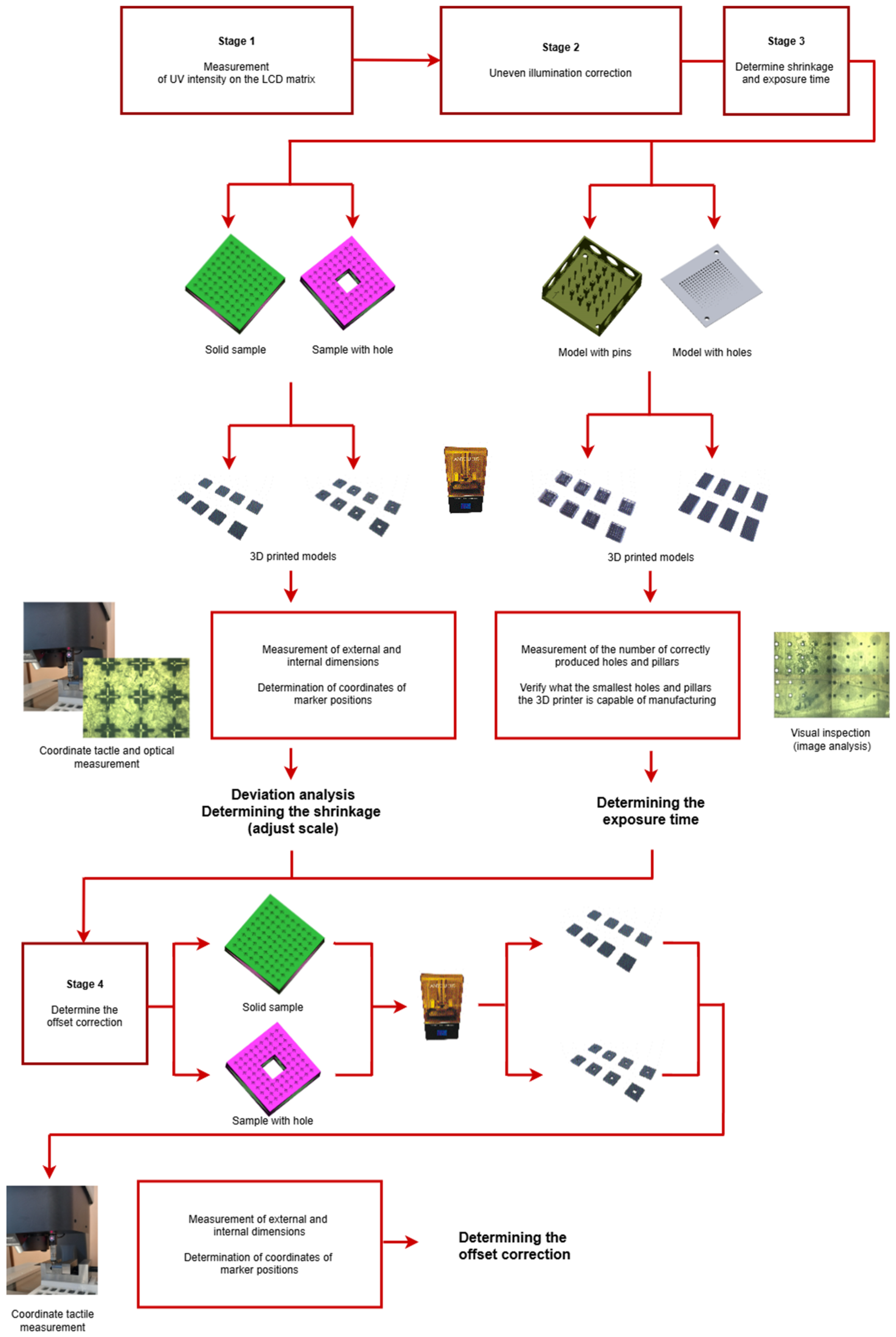
The research process was carried out in several stages (
Figure 1). The first consisted of measuring UV intensity on the LCD matrix and uneven illumination correction of an mSLA Anycubic M3 Premium 3D printer (Shenzhen Anycubic Technology Co., Ltd., Shenzhen, China). The second step consisted of designing models for calibration in NX-Siemens 2406 software (Siemens Digital Industries Software, Plano, TX, USA)
. The developed models were then manufactured on an mSLA Anycubic M3 Premium 3D printer. In the next step, the accuracy of the obtained models was verified using a contact and optical coordinate measuring system. The final step used the measurement results to determine exposure time, shrinkage correction, and offset.
2.1. Measurement of UV Intensity on the LCD Matrix
The Chitu Systems UV Meter For Resin 3D Printer P405L1 sensor with a GVBL-S12SD sensor (Shenzhen Anycubic Technology Co., Ltd., Shenzhen, China) was used to measure the actual UV intensity distribution on the 3D printer’s die and co-curving chamber. The sensor is 36 mm × 36 mm, and the test hole with the sensor has a diameter of 10 mm. The claimed accuracy is 10%. Although the manufacturer provides a full-scale accuracy of ±10%, this parameter is less relevant for evaluating the uniformity of UV illumination across the printing area. Instead, the repeatability of the sensor (i.e., the standard deviation of repeated measurements) is more appropriate for this purpose. Therefore, following the guidance of ISO 5725-2 [
27], we performed a Type A evaluation based on 31 consecutive measurements at three representative locations (center, upper-left, and lower-right corners of the platform). The resulting standard deviation was estimated as 0.0086 ± 0.0011 mW/cm
2, corresponding to a relative uncertainty of 13% in the standard deviation estimate. The measurement range is 0 to 50 mW/cm
2 without using an aperture. Increasing this range is possible using the included aperture, which transmits 3.3% UV radiation. Considering the sensor data and the size of the LCD matrix, the actual measurement step was determined by determining the number of rectangles with the desired length of the eR sides so that an even distribution of measurements across the array was obtained according to Equation (1). The sensor was positioned so that the center of the measurement hole coincided with the center of a single grid box.
—assumed measurement step [-],
Δx—total screen width [mm],
Δx mod —the remainder of dividing ∆x by ,
—number of complete segments of length.
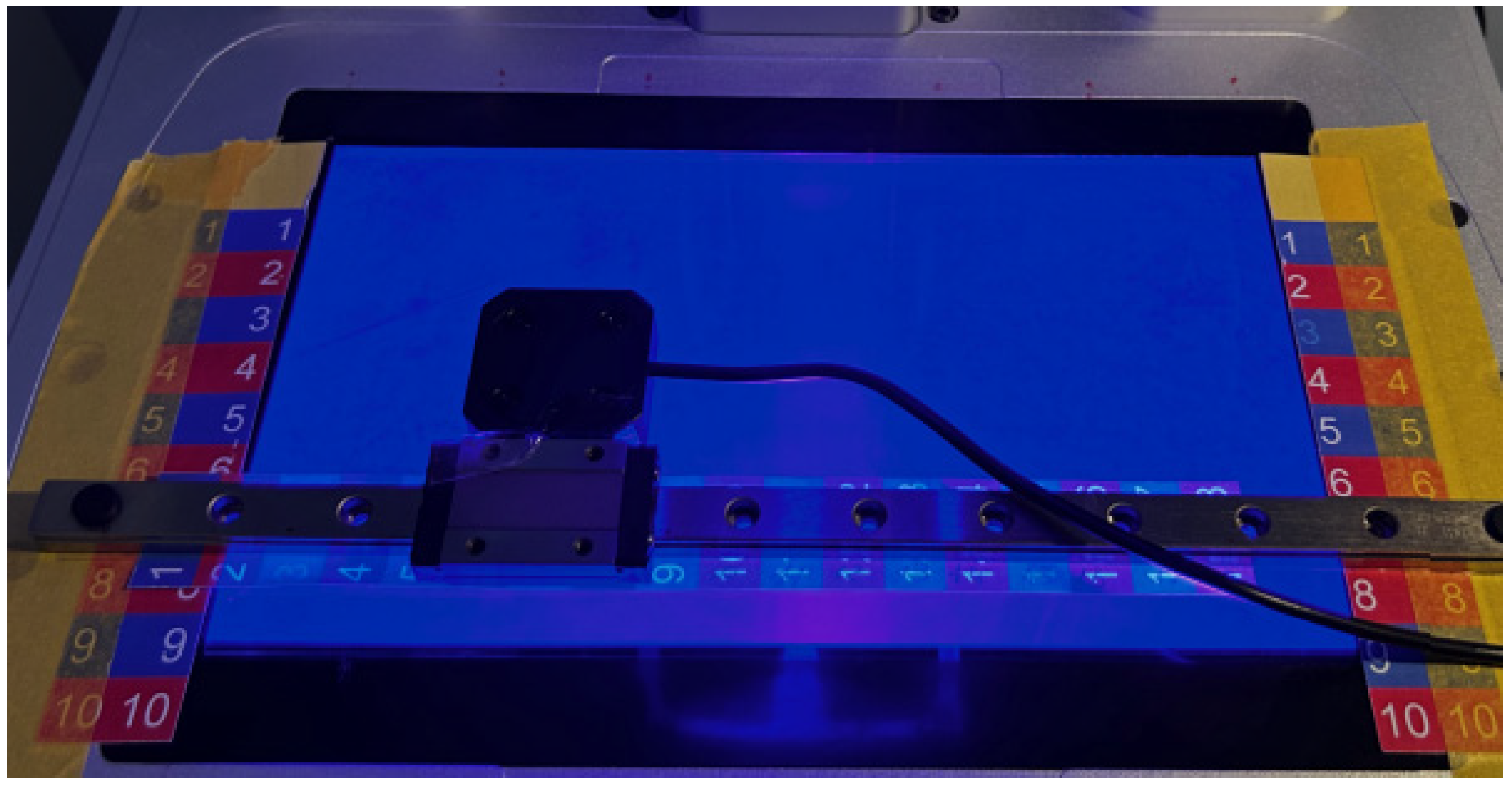
The sensor was positioned using the determined 18 × 10 marker grid manufactured based on calculations and a linear guide with an MGN12 carriage (
Figure 2), to which the UV sensor was attached.
Considering the size of the sensor’s measurement aperture and the design of the 3D printer’s optical system, it was deemed that a positioning accuracy of around 1 mm was sufficient. Possible measurement errors resulting from sensor offsets of 1 mm should not be significant. Additionally, we do not expect the occurrence in this system of local increases in radiation intensity at the merging boundary, as in systems where a grid of UV lamps arranged parallel to the LCD array with collimating lenses is used.
2.2. Uneven Illumination Correction
The illumination of the LCD matrix through which light passes is only approximately uniform. One observes local increases and decreases in the intensity of the radiation penetrating the matrix at different points on the matrix. A mask with a chromatic display can be used in mSLA printers, which superimpose shades of grey on the layer images generated as black-and-white fields. This means that, instead of displaying white fields in which the matrix transmits UV light, locally slightly darkened fields are shown to compensate for the intensity of UV light reaching the resin. To carry out the correction, a test was carried out, which consisted of determining UV intensity measurements at a single point on the matrix for different greyscale values (brightness levels) in increments of 1 from 255 to 199. Three UV intensity measurements were taken for each brightness level. The UV Tools program was used to carry out the test, whereby the appropriate brightness level was set for each layer using the ‘Pixel Arithmetic’ option. These three measurements indicated that the brightness was changed every three layers. Thus, the screen was switched off between each measurement. The file was created from the file generated by the slicer; however, as the option “Apply to: All” was selected, all pixels were converted to the color corresponding to the brightness in question. Based on these measurements, a test was designed in which the brightness was changed between 255 and 110. This time, however, the brightness of layer n was calculated according to Equation (2):
2.3. Design of Calibration Models
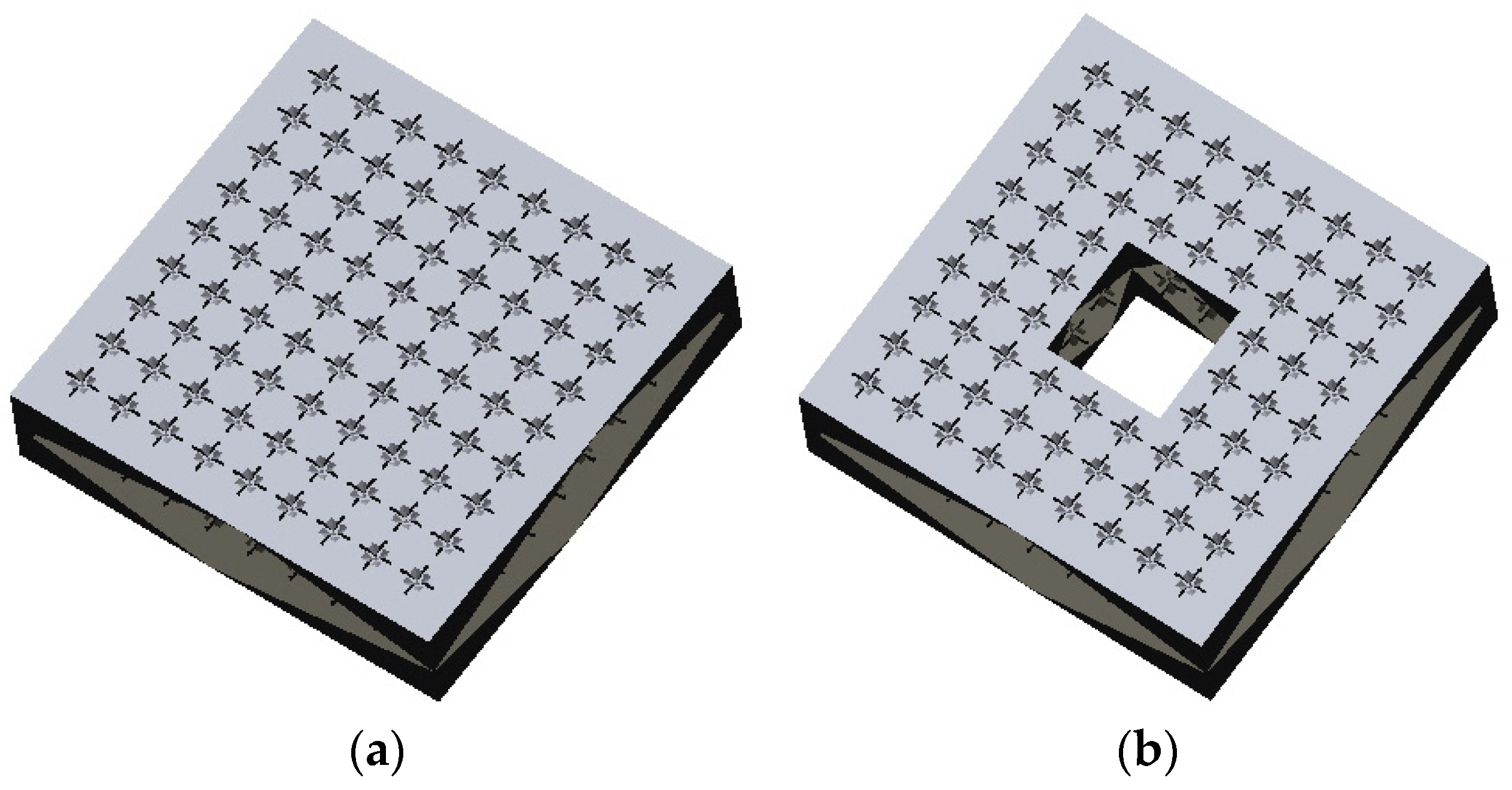
In the study, two pairs of calibration models were developed. The first pair of models aimed to determine shrinkage and offset. The second pair was used to identify the optimal exposure time
t, taking into account the strength and detail of the 3D print. Two calibrator models were used to determine shrinkage and offset. The first consists of a square plate with 25 mm × 25 mm dimensions (referred as the solid sample) (
Figure 3a), while the second also contains a square-shaped hole with a side length of 7 mm in the center (referred as the sample with hole) (
Figure 3b). On both calibrators, markers were placed in square holes measuring 1 × 1 mm and 0.5 mm deep. The corners of the hole were inclined by adding a 0.5 mm chamfer. A marker was also added as a cross with arms 0.2 mm wide and 0.4 mm deep, with the center at the midpoint of the square hole. In this way, the marker’s center can be determined precisely during optical measurement.
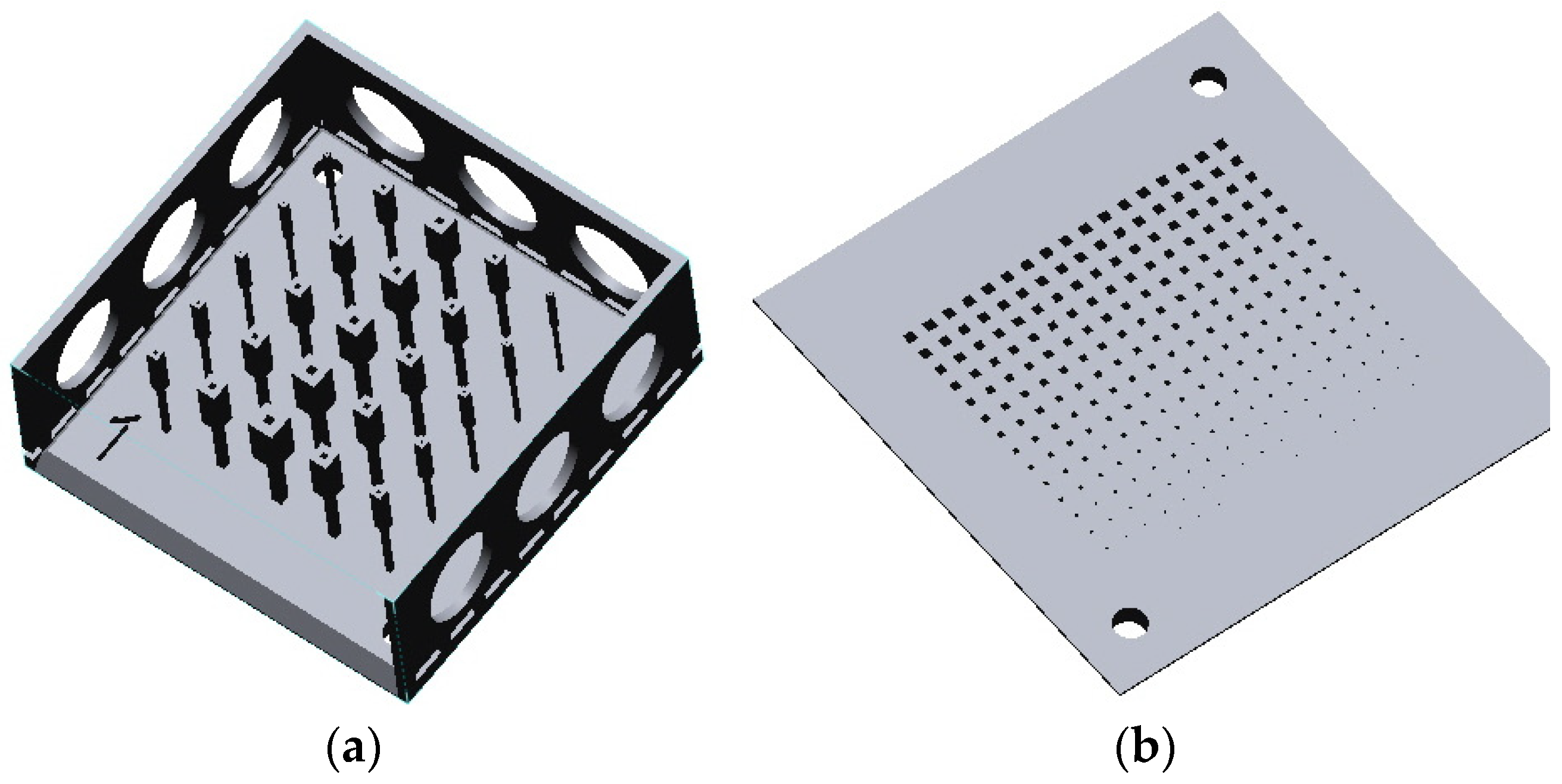
The next set of calibration models were designed to test the effect of exposure time
t on the strength and detail of the 3D print. The calibration models were modeled using NX-Siemens software. Based on Anycubic’s calibration model, the calibrators consist of a 24 mm × 24 mm square plate. The calibrator for determining model strength consists of 5 rows of pins whose diameter decreases with a resolution corresponding to the width of a pixel, i.e., 28.5 µm (
Figure 4a). The biggest pin is located in the middle row. Its dimensions are 1.5 mm × 1.5 mm × 7 mm. The pin is constructed so that 4 mm from the base is narrowed to 0.6 mm. The range of diameters used was determined experimentally. Using pins that are too thin makes them unable to stay on the platform, regardless of the exposure time. Conversely, pins that are too thick do not contribute any relevant information. The pin described above is a base pin duplicated using a symmetrical array. Thus, the right and left rows are symmetrical relative to the middle row. In contrast, the diameter of the subsequent pins in the rows decreases by the pixel’s width to a width of 0.1995 mm. The calibrator with thin sheath pins is used on three sides, which is easily detached from the base to make it easier to grip the sample during post-processing and reduce the risk of damage to the pins during rinsing. It is assumed that, if the pin, despite this sheathing, cannot survive the rinsing process, it is not counted as part of the set of pins correctly manufactured when evaluating the sample. As fine pins are repeated twice, assessing whether damage results from chance is possible. The calibrator for determining model detail consists of a matrix of holes, where, in one direction, the characteristic dimension is reduced from 0.8 mm to a size of 0.342 mm (
Figure 4b) with a step of twice the pixel width. In the other direction, one dimension is reduced by an additional pixel width, causing a transition from a square to a rectangular shape. Consequently, the smallest hole is 0.342 mm × 0.114 mm, which is placed in the opposite corner to the largest hole. The thickness of the calibrator base is 2 mm. A hole is considered to be reflected correctly if light shines through it.
In exporting 3D-CAD models to a 3D-STL model for NX-Siemens software, the accuracy of the generated model is influenced by parameters related to angular and chordal tolerance. To achieve a balance between the accuracy of the 3D-STL model generation and the capabilities of the mSLA Anycubic M3 Premium 3D printer used in NX Siemens software, it is best to undertake the following:
Select the binary format for STL file storage (the American Standard Code for Information Interchange (ASCII) format generates a larger file size);
Set the chordal tolerance to a value of 0.0025 mm;
Set the angular tolerance to a value of 1°.
2.4. 3D Printer and Manufacturing Parameters
The mSLA Anycubic M3 Premium 3D printer was used in the study (
Figure 5). The 3D printer has a monochrome LCD matrix of 10.1 inches and a 7680 × 4320 pixels resolution. The available working area on this 3D printer is 218.88 mm × 213.12 mm, and the pixel size is 28.5 µm. Considering this, the smallest voxel with an assumed layer thickness of 0.05 mm can be 0.0285 mm × 0.0285 mm × 0.05 mm. Hence, obtaining the smallest detail with a characteristic size of about 0.03 mm is theoretically possible.
The matrix in the Anycubic M3 Premium 3D printer is indirectly illuminated by a lamp that emits UV radiation with a wavelength of 405 nm. A concave mirror reflects the UV radiation. As a result of this reflection, an even and perpendicular illumination of the LCD matrix is obtained. According to the specification, UV light power is 7.8 mW/cm
2. As for other parameters, the backlight uniformity expressed in absolute terms is 36.205 mW/cm
3 (90%), the collimation level is 3°, and the stray light level is 1.26%. In the 3D printer, a 10.1″ (218 mm × 122.3 mm) Anycubic Screen Protector film with a thickness of 0.1 mm and a claimed transmittance of about 96.9% is applied to the die. In addition, an FEB film with a thickness of 0.15 mm (actual, measured value) is used as the bottom of the vat. The study utilized Anycubic ABS-Like Resin Pro 2 resin (Shenzhen Anycubic Technology Co., Ltd., Shenzhen, China), and the manufacturer provided the recommended manufacturing parameters for the 3D printer model used (
Table 1).
However, we know from experience that the value of the parameters given by the manufacturer is imprecisely fixed, which means that some 3D prints often fail. Therefore, we treat these as the starting parameters for calibration. We developed our 3D printer settings. Only minor modifications have been made to the manufacturer’s data. Layer exposure time is assumed to be 2.25 s. Light-off was increased to 1 s, thereby minimizing trapped-bubble defects and improving layer thickness uniformity. The number of bottom layers was increased to 3, and 6 intermediate layers were used. No anti-aliasing was used. Advanced platform lift speed control was used. The lift speed for the first 2 mm from the bottom of the vat was 70 mm/min, then 360 mm/min for a distance of 8 mm (+6 mm). Access to the platform is 2 mm from the bottom of the vat at 360 mm/min. The last section of the approach was performed at a speed of 140 mm/min. During the tests, the temperature in the 3D printer chamber was kept constant at 28 degrees. As the temperature of the resin increases, its viscosity decreases. This facilitates the flow of resin from the workpiece into the vat and reduces the force exerted by the squeezed resin when the platform reaches the screen, especially for the former, where there are very short distances between the platform, which is a uniform flat aluminum surface, and the bottom of the vat. The chamber was heated up to the set temperature 15 min before the start of printing to allow time for the temperature of the printer components and resin to stabilize. No tests were conducted to determine whether this is enough time to achieve the desired effect. However, a longer time would be impractical and increase power consumption. As the Anycubic M3 Premium printer does not have a heated chamber, an external Chitu Systems H2 3D Printer Mini Heater was used to heat the chamber. This heater has a temperature sensor and controller that automatically maintains the ambient temperature.
In manufacturing the calibration models presented in
Figure 2 and
Figure 3, a function built into the Anycubic 3D printer software version 3.5.0 (Shenzhen Anycubic Technology Co., Ltd., Shenzhen, China) was used. This function recognizes the calibration file named “R_E_R_F.” (
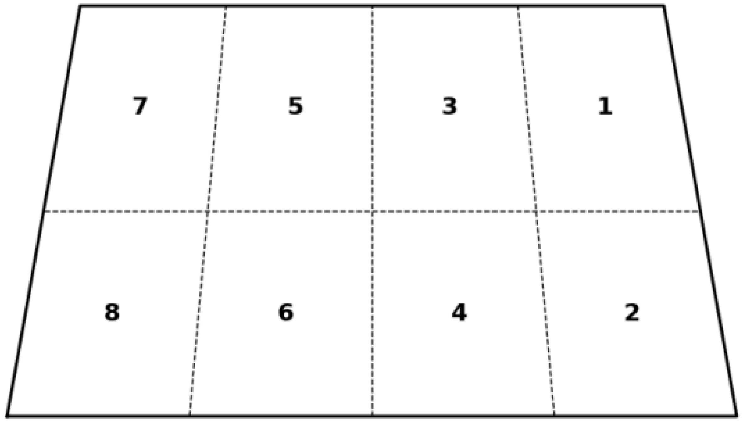
Figure 6). This mode divides the screen into eight parts, creating a 2 × 4 grid. Elements arranged in the first area are 3D printed with an exposure time of 2.25 s (values adopted in the research process). Subsequent regions are faded, with a delay of +0.25 s relative to the previous one. This way, models for eight different exposure times from 2.25 s to 4.25 s were obtained in one manufacturing process. Each set of calibration models (with 8 different exposure times) was printed twice.
The study utilized a Formware 3D slicer 1.0.2.6 (Formware B.V., Amsterdam, The Netherlands) To better mimic natural 3D printing conditions, all samples for testing were created on supports. The support settings are detailed in
Table 2.
2.5. Measurements and Data Analysis
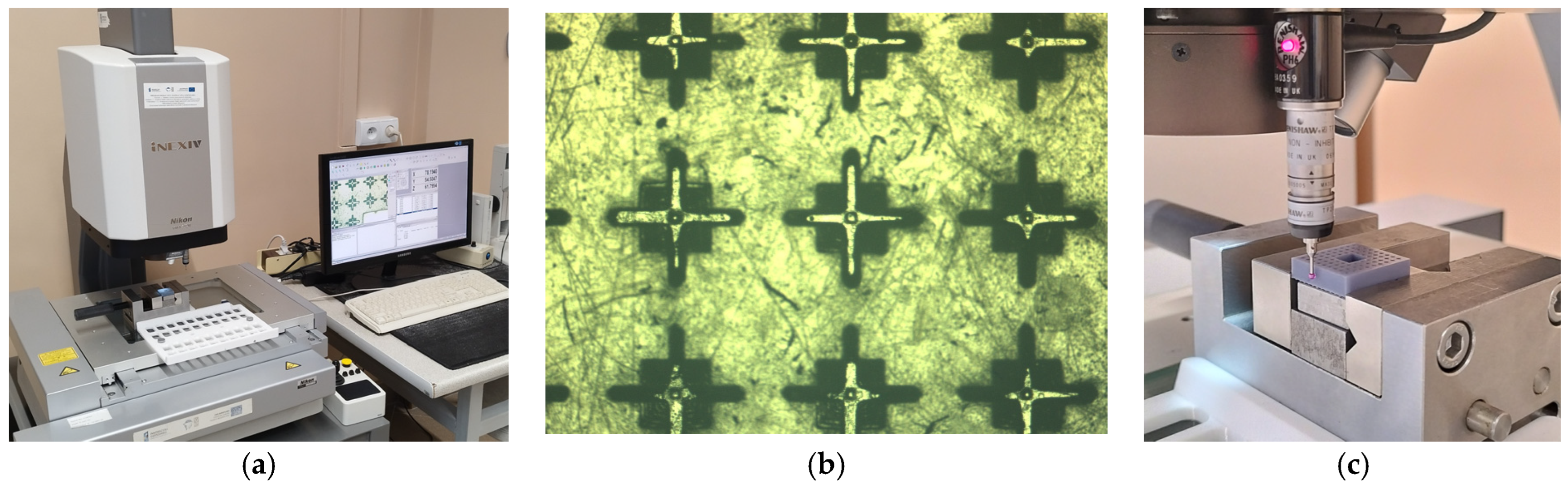
All geometric measurements of the 3D printed samples were performed using the iNEXIV VMA-2520 vision system (Nikon Metrology Inc., Tokyo, Japan) equipped with a Renishaw
® TP20 touch probe (Reinshaw, New Mills, Wotton-under-Edge, Gloucestershire, UK). For the samples used to determine shrinkage and offset, the coordinates of the marker centers were measured using the cross function by manually indicating the position of each point (
Figure 7). The measured coordinates of the marker centers were exported to an XPS file and further analyzed using the Python 3.12.7 (Python Software Foundation, Wilmington, DE, USA) programming environment.
Based on the points nominally lying on the vertical and horizontal axes of symmetry, regression lines were determined. The intersection point of these lines was taken as the center of the sample, relative to which the nominal positions of the measured points were defined. Knowing both the nominal and the measured positions of the marker centers made it possible to determine the displacements caused by material shrinkage.
The external dimensions of the samples along the X and Y printing directions—nominally 25 mm—as well as the size of the square hole (with a nominal value of 7 mm) were measured using the touch probe (
Figure 7). The declared maximum permissible error (MPE) for touch probe measurements is 3 + 8 L/1000 µm.
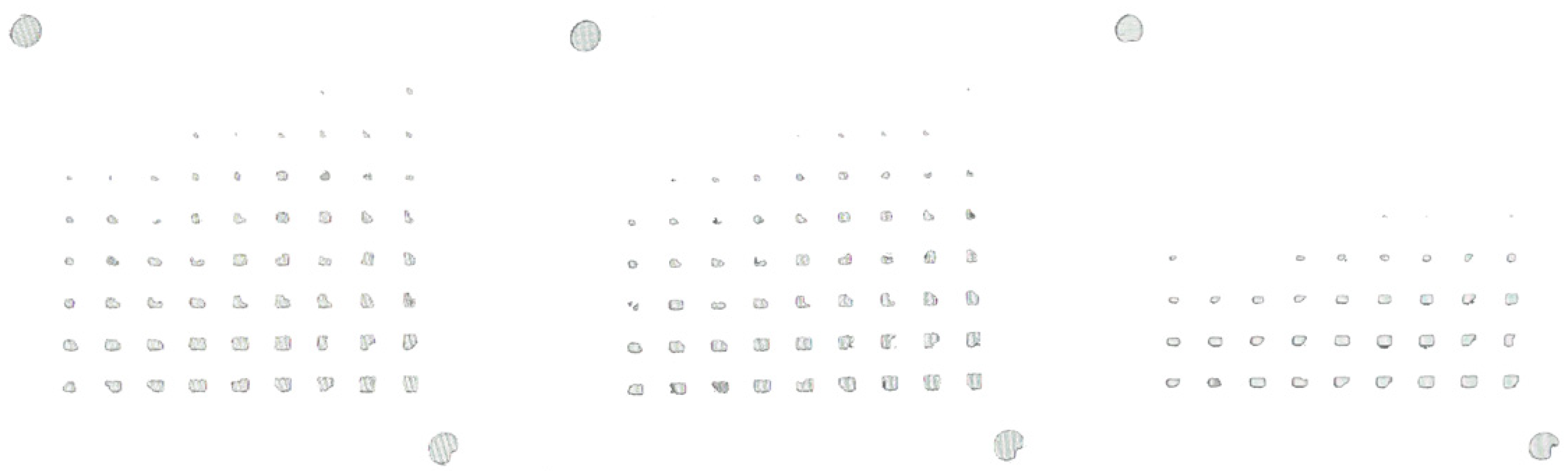
For the models used to determine exposure times—i.e., the model with pins and the model with holes—the correctly printed pins and holes were counted. A pin was considered correctly printed if it was not tilted. To facilitate hole counting, the models were placed on a backlit LCD screen and photographed. Then, in Affinity Photo 2, dark areas were replaced with white using the “Flood Fill Tool,” making the holes easily visible.
A statistical analysis of the test results was performed using JMP 12.01 software (SAS Institute, Cary, NC, USA). In all tests, a significance level of alpha = 0.05 was used.
3. Results
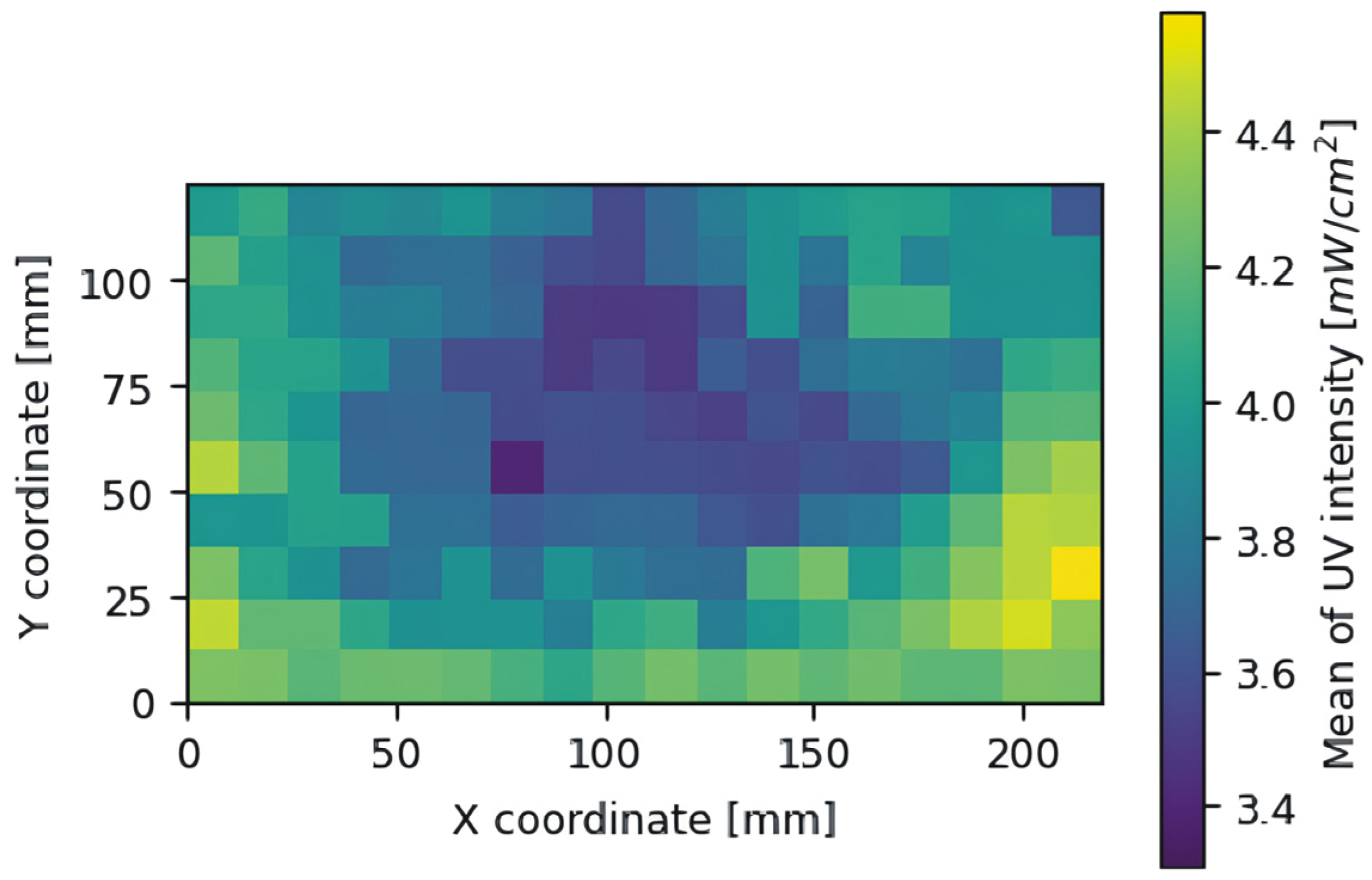
3.1. Calibration of the UV Illuminance Uniformity
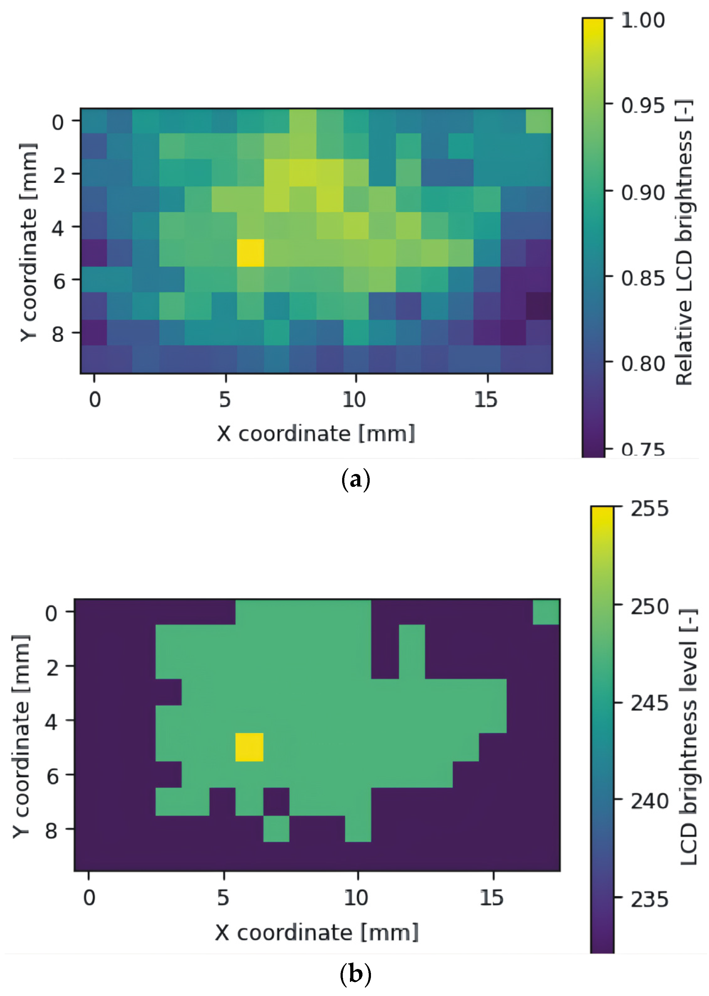
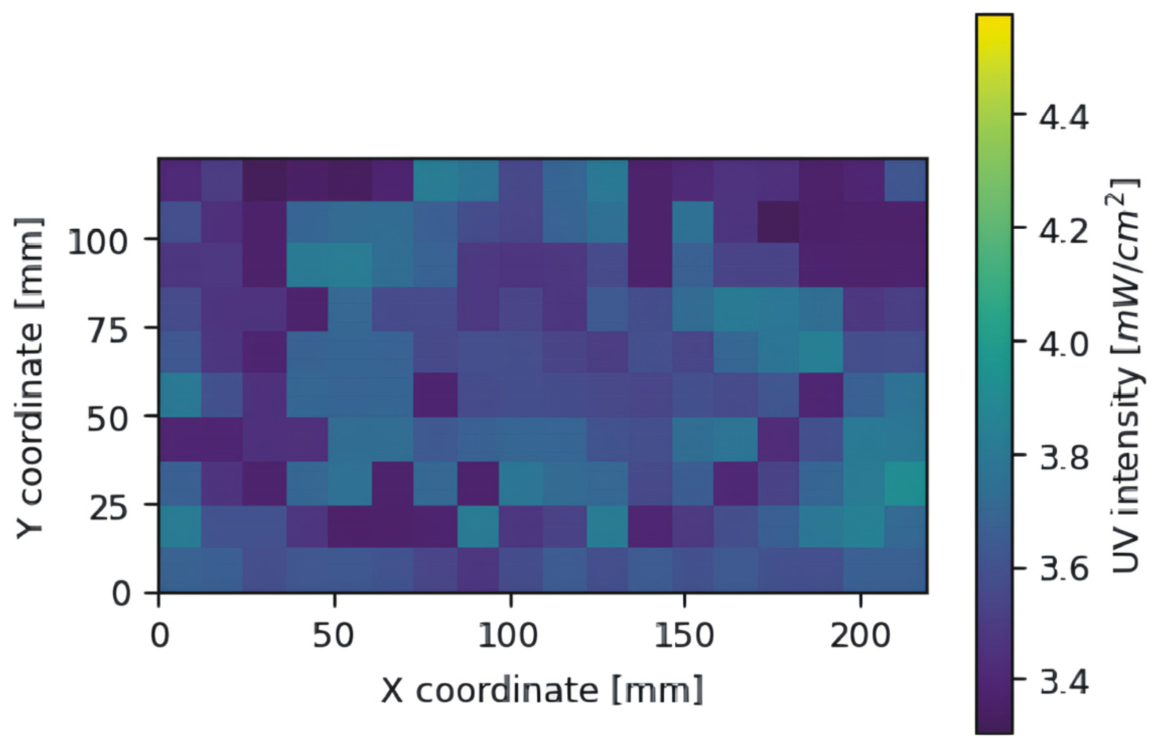
Calibration of the UV illuminance uniformity was undertaken by generating a greyscale mask. Typically, the brightness can be set in an 8-bit greyscale from 0 to 255. However, this does not mean the LCD matrix can display all shades of grey. In addition, it is also not clear that the intensity of the transmitted UV radiation is proportional to the greyscale value. Therefore, the following measurements were taken initially:
UV intensity distribution on the LCD matrix,
Figure 8;
UV intensity as a function of greyscale at selected measurement points,
Figure 9.
In the research for this article, measurements were taken with a resolution of approximately 12 mm (measurement grid with 18 columns and 10 rows).
It is not difficult to see that, in the case of the Anycubic M3 Premium 3D printer used in the study, the radiance intensity does not change with a resolution of every one greyscale unit.
To evaluate whether the 12 mm measurement grid spacing significantly impacted the accuracy of the final correction mask, a high-resolution scan was conducted over a 31 mm segment, which includes more than two full standard grid areas. The scan was performed at coordinates x = 60 to 91 mm and y = 50 mm, in a region previously identified on the irradiance map as exhibiting high local variability. In our printer, the UV exposure system consists of a single collimated lens with a custom-shaped reflective mirror. This design is intended to provide uniform light distribution without the overlap of artifacts commonly observed in systems using multiple parallel lens arrays (as found in some MSLA printers with tiled LED modules). In those systems, narrow bands of elevated irradiance often occur at the interfaces between adjacent light sources, leading to sharp local peaks in UV exposure. In contrast, the optical system used here is expected to produce smoother irradiance gradients. Based on the high-resolution scan and visual inspection of the irradiance map, we estimate that the spatial interpolation error does not exceed 0.05–0.1 mW/cm2 because of the use of a grid of 12 mm instead of 1 mm, which remains below the minimum effective correction step of the LCD panel and therefore has no practical impact on the correction mask generation.
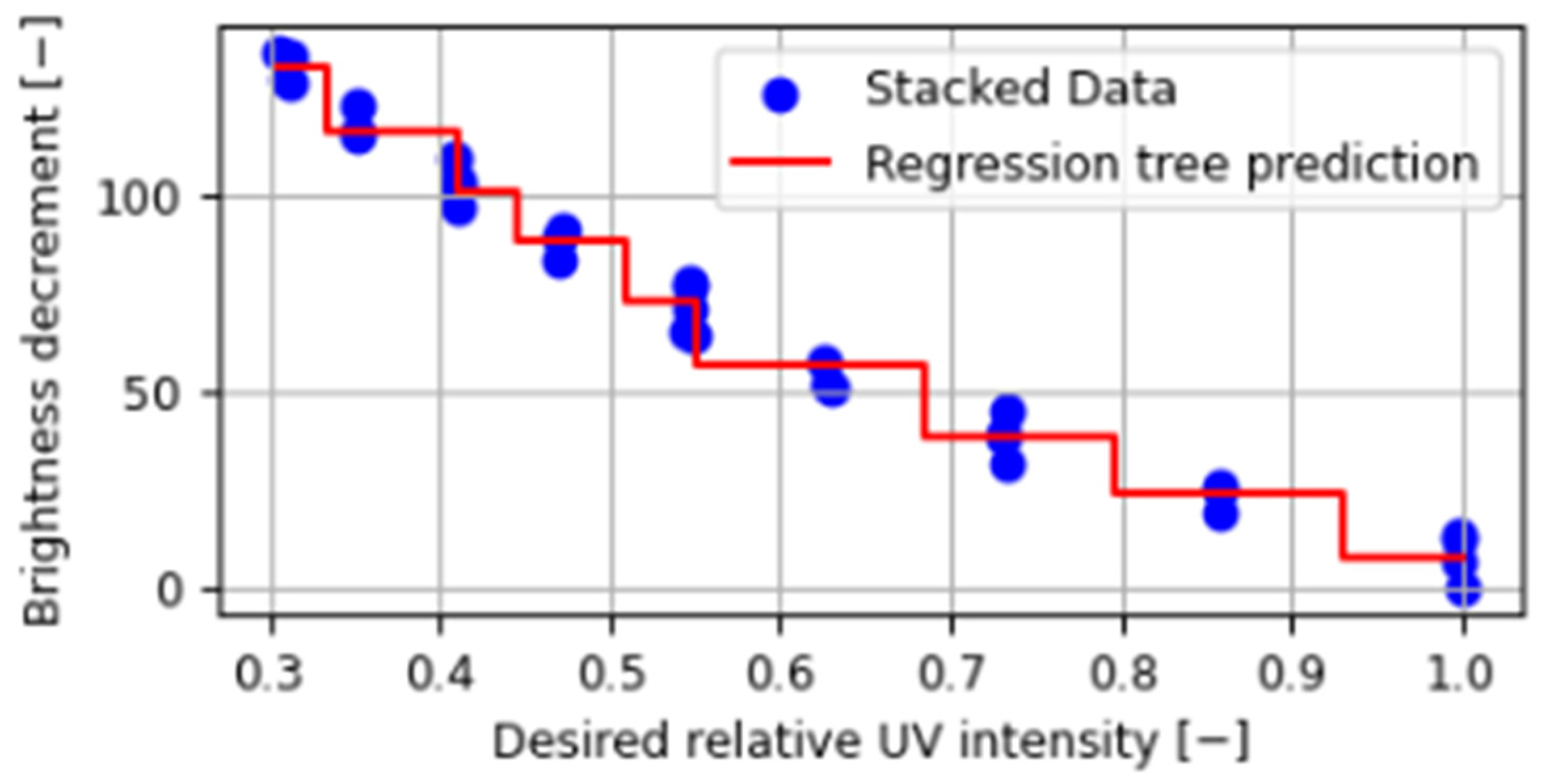
As the change is stepwise and not linear, a tree regression model was determined for further calculations (
Figure 10).
However, to use this model for further calculations at any point in the matrix, the values of the measurements were normalized against the maximum value (3), as follows:
As the waveforms are very similar, it was assumed that the model would be created using the data from row 2 and column 17. For convenience, the model operates on values relating to the reduction in brightness of the LCD matrix. That is, the value of adjustable brightness is 255—∆b
n. It was also necessary to develop a model to determine the value by which the brightness intensity of the LCD matrix should be reduced to achieve the expected relative UV (
Figure 11).
Based on the application of the models described above, maps were determined as follows:
The LCD matrix’s expected relative brightness correction value (
Figure 12a);
Brightness values consider the constraints on the brightness adjustment of the LCD matrix (
Figure 12b).
These maps generated a greyscale image with a resolution of 7680 × 4320 pixels as a correction mask. Due to the very light shades of grey, it is not included in the article. However, this is just a simple transformation from a color map to greyscale. After applying the correction mask, a map of the brightness distribution of the LCD matrix, as per
Figure 13, was obtained. For ease of comparison, the same scale as in the map was used with the values measured before correction (
Figure 8). The correction mask was applied using UV tools. Repeated measurements of light intensity after applying the correction showed a reduction of the original standard deviation from 0.26 to 0.17 mW/cm
2, representing a decrease of more than one third. Future research may focus on developing alternative methods for correcting non-uniform illumination that would overcome the limitation caused by the limited number of effective brightness levels available for LCD control.
3.2. Determination of Linear Shrinkage
Using the iNEXIV vision system, the
x and
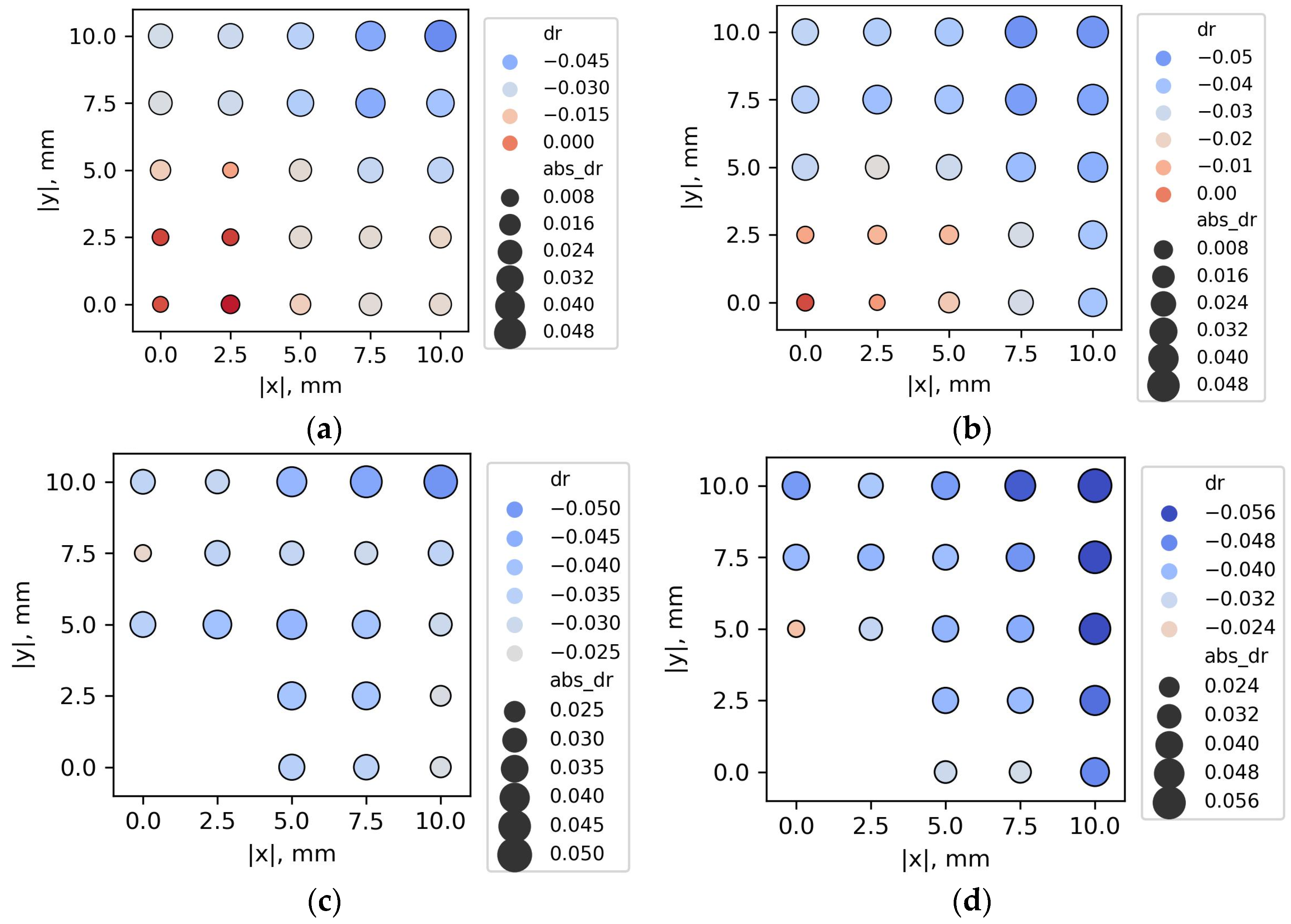
y coordinates of the marker centers were measured on samples marked with crosses. Based on these measurements, the primary parameter analyzed in the study was the resultant displacement (
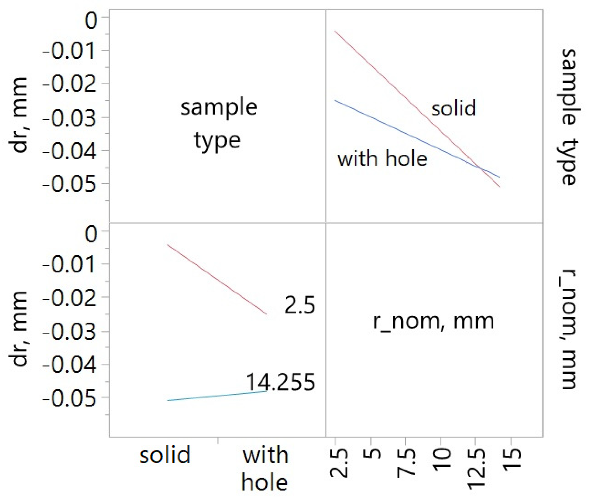
dr) of the measured point from its nominal position. Positive values of the determined displacement indicated that the measured points were located farther from the center of the sample than their nominal positions suggested. Negative values, on the other hand, indicated that the points had moved closer to the center. The axes of symmetry divided the samples into four quadrants. The obtained
dr values were averaged for corresponding points from different quadrants. The results, presented graphically for the solid plate and the one with a hole, for the shortest and longest exposure times, are shown in
Figure 14.
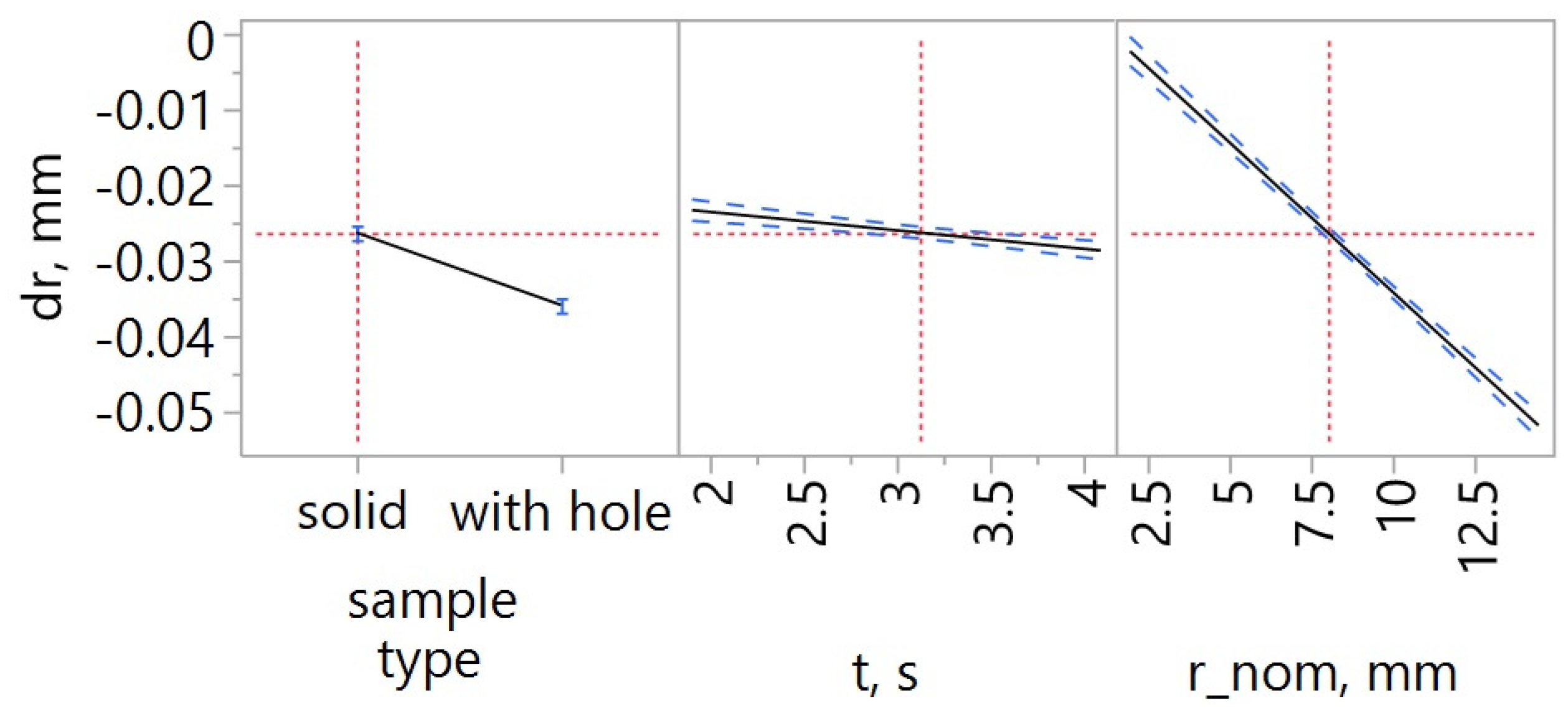
To determine the influence of sample type (solid and with hole), exposure time (
t), and the nominal distance of the marker from the center of the sample (
d_nom) on marker displacement (
dr), a regression model was developed that included linear effects and two-factor interactions. Using a significance level of α = 0.05, backward regression was performed. In the final model, all three examined factors, as well as the interaction between sample type and exposure time, were found to be statistically significant (
Table 3). The model was statistically significant but exhibited moderate fit (adjusted coefficient of determination R
2adj = 0.70). Therefore, the model can be used to identify dominant trends and relationships between factors—which was the purpose of its development—but it is not suitable as a predictive model. The influence of the studied factors and the interaction effect are presented in
Figure 15 and
Figure 16. The most significant influence on marker displacement due to shrinkage was the marker’s distance from the center of the sample. As expected, the farther the marker was from the center, the greater its displacement. Larger displacements were observed in samples with a hole, due to the increased unconstrained shrinkage in those samples. However, the interaction plot reveals that differences between the samples with and without a hole are evident mainly for markers located near the center. Displacements of the markers at the sample edges were comparable regardless of sample type. The longer the exposure time, the greater the marker displacement, and thus the shrinkage.
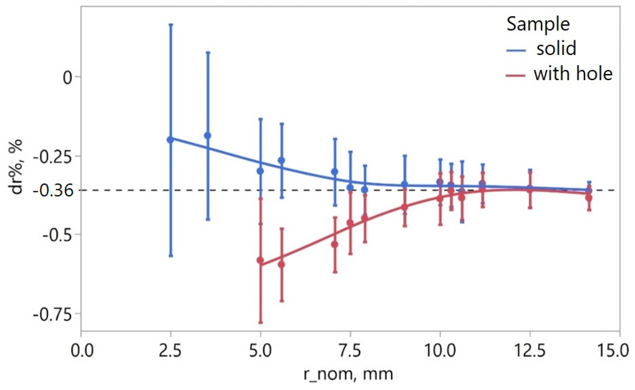
To calculate the correction for dimensional changes of the samples due to shrinkage, the relative displacement of each marker was first calculated using the following formula:
In
Figure 17, which shows the relationship between relative displacement and sample type as well as the distance of the markers from the center of the sample, it can be observed that the differences in relative marker displacement (dr%) between different sample types decrease as the nominal distance (r_nom) increases. For r_nom > 10 mm, the differences in dr% stabilize at approximately −0.36%. This value was determined as the median of the dr% values for both solid and hole samples. For the purpose of determining the shrinkage value to be set in the printing settings for solid samples, the linear shrinkage was assumed to be s = 0.36%, corresponding to the overall shrinkage of the sample. Shrinkage and its potential compensation concern only the external contour. The case of the sample with a hole is more complex. The displacement of markers at the external contour relative to the nominal value differs from the displacement of markers at the internal contour. To compensate for shrinkage, the average shrinkage value of s = 0.44% was adopted based on the average dr% value for samples with hole.
3.3. Analysis of Linear Dimensions
The linear dimensions of the samples were measured, including the external dimensions of the full sample and the sample with a hole, as well as the internal diameter of the hole in latter sample.
The measured dimensional error (
dm) is the difference between the measured dimension and the nominal dimension. The dimensional error (
dm) includes, among other factors, the error due to linear shrinkage (
ds) and the error from light bleed. The shrinkage error was determined using the following Equation (4):
The remaining part of the dimensional error (
dl), associated among others with light bleed, was calculated as the difference, as follows:
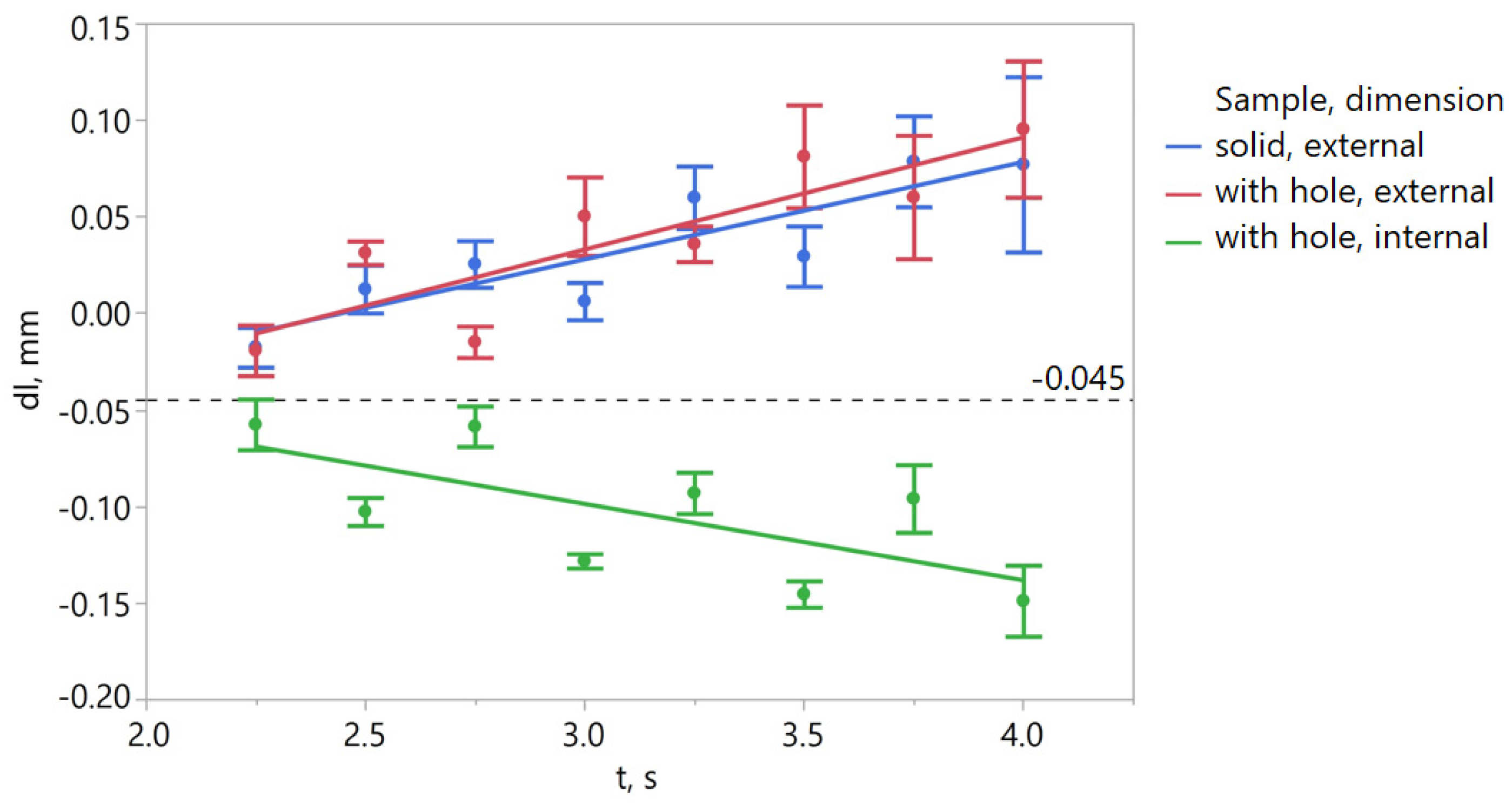
The results of
dl are shown in
Figure 18. The error caused by light bleed should be positive for external dimensions and negative for internal dimensions. Theoretically, as the exposure time increases, light bleed should become larger, and therefore the magnitude of the deviation (its absolute value) should also increase. The results of the tests largely reflect these assumptions. The deviations for external dimensions with short exposure times are negative. This may be caused, among other factors, by printing errors related to matrix resolution and print repeatability.
In
Figure 18, a trend is visible, indicating that the error value depends significantly on the interaction between exposure time and the type of dimension. The error values (
dl) for the external dimension of the solid and hole samples are similar. To investigate the significance of the aforementioned factors on the error value (
dl), a regression model was developed. Through factor significance analysis in regression, the statistical significance of factors such as dimension type and the interaction between exposure time and dimension type on the value of
dl was confirmed (
Table 4). The variability of these parameters accounts for 88% of the total observed variability in the
dl parameter. The influence of sample type on
dl was not statistically significant.
For the samples with hole, the error
dl (
Figure 18) for the external dimension is not symmetrical around zero (it is symmetrical around the value of −0.045), so it cannot be easily attributed to light bleed. The values of contour shifts relative to the nominal dimension result from the combined effects of shrinkage and light bleed. Therefore, to compensate for dimensional errors, it was proposed to first compensate for shrinkage (samples labeled as scaled). After measuring the dimensional errors
dm on the scaled samples, an appropriate offset can be determined. This procedure has been verified, and the results of this verification are presented in
Section 3.5. An extension of this research area related to improving the accuracy of printed models could be concerned with the reduction of shrinkage and offset correction steps into a single stage.
3.4. Determine the Optimal Exposure Time
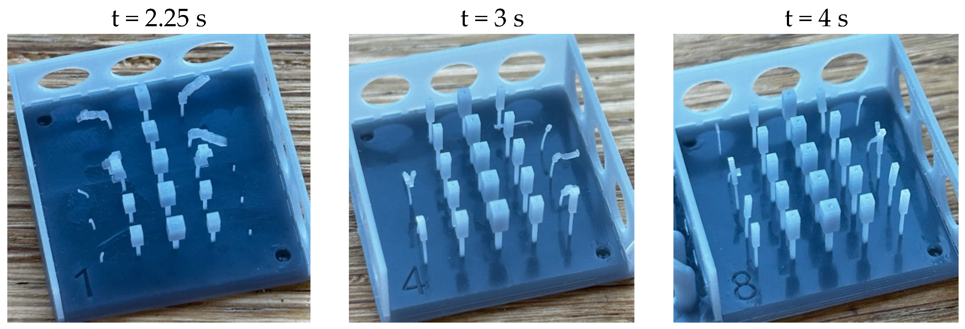
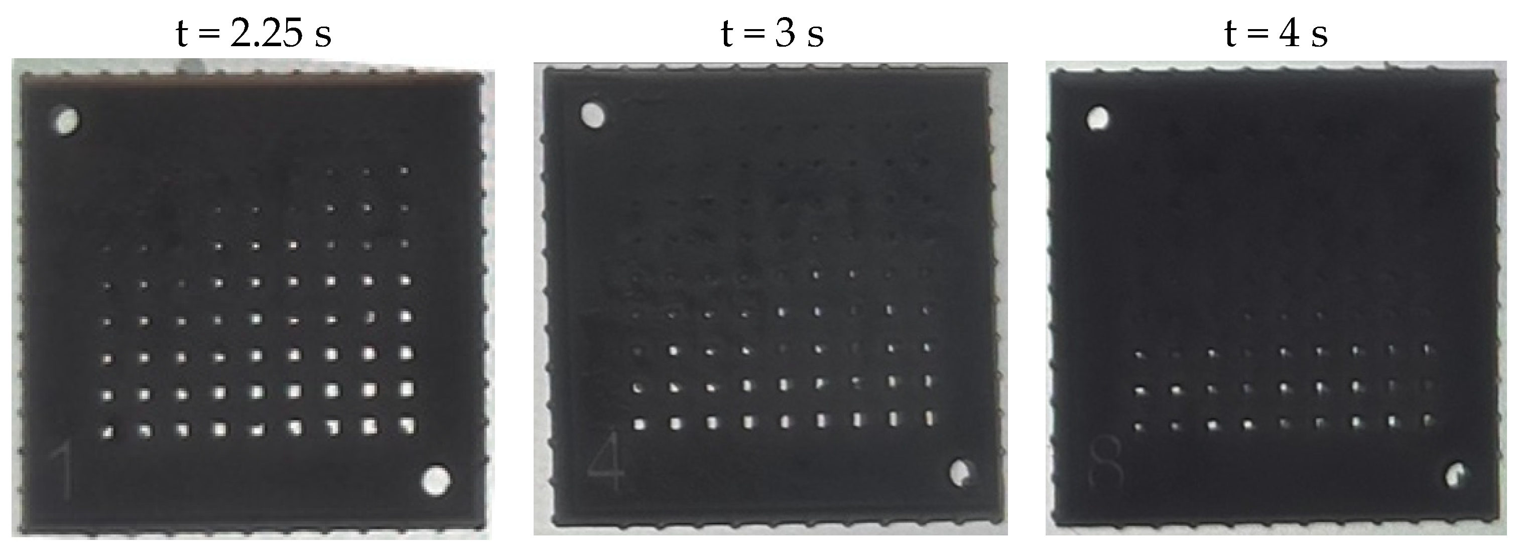
The optimal exposure time was determined based on the analysis of samples containing a series of pins and holes.
Figure 19 and
Figure 20 show samples printed with the shortest and longest analyzed exposure times, as well as with a time of t = 3 s, which was identified as optimal based on the study (as will be presented later in the article). The darker color of the samples with holes is due to backlighting from below to make the holes more visible. The holes were processed in Affinity Photo 2 by filling the dark color with white using the “Flood Fill Tool” (
Figure 20).
Based on the measurements of the number of holes and pins, an optimization process was carried out, where the objective function was to maximize the number of holes and pins. It was assumed that holes and pins were considered equally significant in the decision-making process. The dependence of the number of pins and holes on exposure time was modeled using quadratic functions. The prediction profiler for the functions for the number of holes(t) and number of pins(t), along with the desirability function, is presented in
Figure 21. As expected, the number of holes decreases with increasing exposure time, primarily due to greater light bleed. On the other hand, a longer exposure time results in a higher number of correctly printed pins, as the resin is more fully cured. The optimal time determined from the objective function was approximately 3 s (2.99 s).
3.5. Verification of the Study
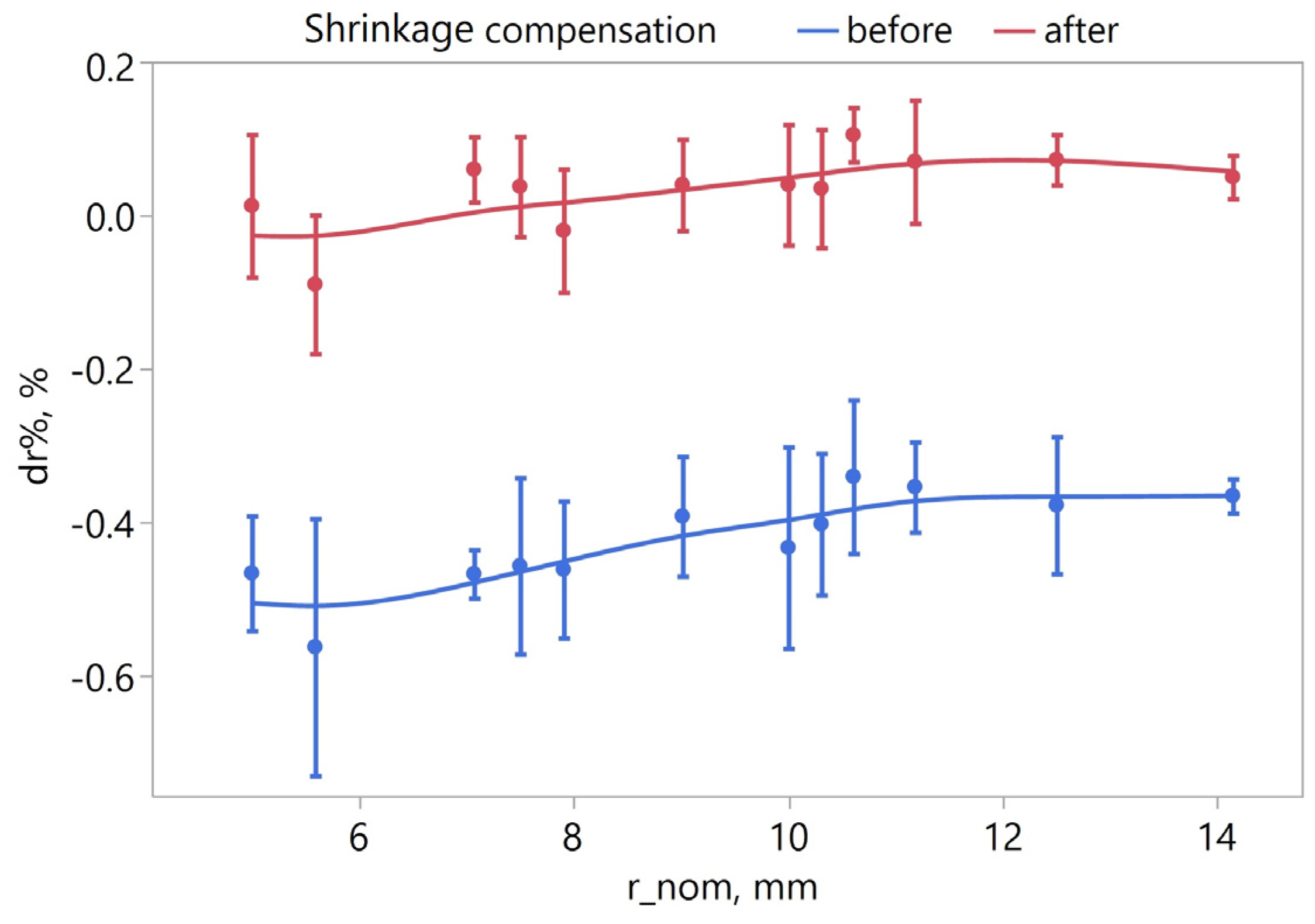
Due to the greater complexity of the geometry and the asymmetrical distribution of deviations, the verification of the shrinkage and linear dimension compensation methodology was carried out on the samples with a hole. To verify the proposed methodology for determining corrections related to linear shrinkage and light bleed, samples with a hole were printed with an exposure time of t = 3 s. To verify the shrinkage correction (s = 0.44%), four samples were printed with a scale of 1.0044 and without defining an offset (referred to as scaled samples).
Figure 22 presents the values of the relative marker shift dr% on the samples before and after the applied corrections. The trend line for the samples after linear shrinkage compensation clearly shifted toward the value of 0. The average value of the dr% indicator for the samples after compensation was 0.003%.
The last step was to check the linear dimension compensation procedure. To compensate for dimensional errors, it was proposed to first compensate for shrinkage. After measuring the dimensional errors on the
scaled samples, an appropriate offset was selected. Depending on the slicer used, the offset is either constant for the entire contour, or it is possible to define two different offsets for the outer and inner contours. However, slicers may also differ in the quality of recognizing outer and inner contours. In the study, the most universal option was adopted, i.e., a constant offset—regardless of the geometry type. In the case of analyses without anti-aliasing (anti-aliasing was not the subject of the study), the offset size translates to the number of pixels removed. Knowing the errors of the scaled samples, an offset value of 0.06 was adopted (removing two pixels into the material). Four samples were printed using both the scale factor and the offset correction. The results of scale and offset correction are presented in
Table 5.
The application of the scale increased the external and internal dimensions by 0.095 mm and 0.085 mm, respectively. Applying the offset resulted in a reduction of the external dimension by 0.088 mm and an increase in the internal dimension by 0.057 mm. As before, the different values of contour shifts may result from the interaction between shrinkage and light bleed. Compared with the initial state (without correction), the internal dimension of the sample decreased by about 0.14 mm (over 167%). The reason for the limited correction of the external dimension error was the use of an equal offset for both the outer and inner contours. Reliable quantitative benchmarks for mSLA accuracy are scarce. Nevertheless, in [
28] the authors relied solely on a classical Jacobs working curve calibration and obtained dimensional errors in the range of 40–50 µm. Their experiments were carried out on industrial-grade DLP machines, which intrinsically provide higher XY precision than the consumer class mSLA system used here. Therefore, the accuracy levels achieved in the present work can be regarded as highly promising.
4. Discussion
As functional models are often produced using additive technology, it is necessary to develop guidelines for optimizing 3D printing parameters to create models that meet the requirements for dimensional and shape accuracy and surface roughness. For this purpose, ISO/ASTM 52901 [
29], ISO/ASTM 52902 [
30], and ISO/ASTM 52910 [
4], among others, have been developed. However, the information in the presented standards provides only general guidelines for verifying the accuracy of 3D printers, which in no way directly relate to establishing calibration parameters for 3D printing models also obtained using the mSLA method. Therefore, it was necessary to develop, within the framework of the presented publication, a procedure related to the calibration of a 3D printer using, among other things, individually designed models to establish parameters minimizing manufacturing errors.
For the mSLA method, in particular, it is important to choose the right exposure time [
31] and layer thickness [
32] of 3D printing. In general, the layer thickness is determined according to the recommendations of the resin manufacturer or the type of 3D printer. In practice, it is believed that the value of the layer thickness below 30 µm, does not bring tangible benefits, and unnecessarily increases the time of making the model. Therefore, in the presented research, we maintained the recommended value given by the manufacturer. According to this recommendation, for the mSLA Anycubic M3 Premium 3D printer, the 3D printed layer thickness should be 50 µm. The problem is more complex in terms of determining the correct exposure time. So far, no clear recommendations have been made for determining the value of this parameter. Recommendations contained in publications and provided by manufacturers are usually very general [
15,
16,
31]. The authors of the publications mainly aim at adopting such a value of the exposure time that the 3D printing layer will achieve adequate strength while not curing too deep into a single layer. Determining such a value of exposure time also avoids the overcuring of higher layers, which would lead to excessive increase in stress, brittleness and increase in dimensional and geometry errors [
33]. Commonly available calibration models and calibration instructions are mostly based on subjective evaluation of the detail and strength of prints by observing the fine details of test prints [
20,
21]. However, there is a lack of description of calibration methods based on measurements that give numerical comparison data. In the case of the publication presented here, the authors used two models, one of which was used to evaluate the detail of the print and the other for its strength. The criteria for evaluating the print detail on these models are clear and easy to apply. The preferred exposure time can then be determined based on the optimization criterion. The published literature lacks a comprehensive calibration procedure for 3D printers that utilize the mSLA method [
15,
16,
31]. This paper presents a calibration procedure that includes several key elements: testing the uniformity of UV intensity emitted by the LCD matrix of the Anycubic M3 Premium printer using a grayscale correction mask, determining the optimal exposure time, and assessing the linear shrinkage of samples. One notable advantage of the method presented is its ability to collect and analyze numerical data, reducing the impact of the operator’s subjective judgment—which is often a significant factor in traditional calibration methods. Until now, most verification methods for models created using the mSLA technique have relied solely on visual evaluations, which depend heavily on the operator’s subjective assessment [
15,
32].
Geometric errors in models made using the mSLA method can result from a variety of factors. The most common include errors due to shrinkage of the material, an error resulting from the fact that not all of the radiation falls on the matrix at exactly 90 degrees, and from radiation scattering which results in the formation of a UV light bleed, which acts on the material outside the contour of the mask to cure it [
34]. This results in a mechanism that is intuitively easy to explain, in which the longer the exposure time, the more resin manages to cure outside the contour. This is also how errors arise, causing the printed holes to be smaller than the nominal dimensions and the effect of shrinkage, and the outer dimensions to be 3D printed larger. If the holes are relatively small, this leads to plugging. Analyzing the topic a level deeper, it is not hard to see that illumination time alone is a vague parameter in the context of curing photopolymers. What matters is the amount of energy that must be delivered to cure the resin. Thus, it is important that the entire working area be as evenly illuminated as possible to be able to obtain reproducible 3D printing results regardless of where the object is located on the printing platform. Therefore, it is first necessary to calibrate the illumination intensity of the UV matrix. In this study, such calibration was performed by measuring the distribution of UV intensity on the LCD matrix and an in-house method of analyzing the measurement data leading to the generation of a grayscale mask that can be used to darken the matrix locally, minimizing local irregularities in the intensity of UV radiation curing the resin. As a result, more predictable printing was achieved, which also improves calibration accuracy.
Although the shrinkage value is declared by the resin manufacturer in the specification, this value is not useful for dimensional correction, as the manufacturer usually declares volumetric shrinkage [
34]. When minimizing dimensional and geometric errors in models made using the mSLA method, a more linear shrinkage value is needed. Although this value can be theoretically recalculated according to Equation (7), in practice it is better to determine it experimentally. As shown in the conducted studies, the material displacement associated with shrinkage significantly varies depending on the geometry of the model.
where S
l is linear shrinkage [-] and S
v is volumetric shrinkage [-].
In order to compensate for shrinkage at the slicer stage, a shrinkage study based on the displacement of markers on the test model was proposed. The markers, for which their center is determined, allow one to determine directly the shrinkage value without mathematical elimination of the light bleed effect. This way, errors do not accumulate, so calibration is simpler and more predictable. In order to measure the coordinates of the centers of the markers with the required accuracy, measurements were carried out using the iNexive vision system. Future research can be developed toward using simpler image acquisition and image analysis methods to automate this process.
The discussion presented also mentioned the occurrence of UV light bleed, also curing the resin outside the mask outline. Recent studies have confirmed that the phenomenon of light bleed significantly affects the dimensional accuracy of models printed using the mSLA technology and related methods [
28,
34,
35,
36,
37]. In the research conducted, it was assumed that the effect of light bleed on the inner and outer contours has opposite direction. As a result, the outer dimension is reduced by shrinkage while being increased by light bleed. The inner dimension, on the other hand, is reduced by both shrinkage and light bleed. It is this difference that results in dimensional error asymmetry. Errors due to shrinkage depend on the value of the nominal dimension, so their compensation should be carried out by means of a scale factor. The effect of light bleed, on the other hand, is independent of the size of the detail, and thus cannot be fully compensated for by scaling. It is also worth noting that scaling changes the position of details on the surface of the model, while offset alone only modifies the size by shifting the outline in the perpendicular direction by a given value. Therefore, compensation by offset alone is not a universal method. For this reason, it is recommended to first carefully select the scale and only then set the offset value. In more advanced slicers it is possible to set the scale and offset. In general, the operation is such that first the object is scaled. This is undertaken at the 3D model level. Then, in post processing and after generating layers, pixels are subtracted from the inner and outer contours depending on the offset value. Often, slicers allow you to define the offset for the outer and inner contours separately. However, a difficulty arises in classifying them unambiguously. Internal offsets usually refer only to closed internal contours, which can lead to unexpected results. Hence, the study adopted a single offset value, regardless of the type of geometry. Taking into account the above considerations and the experimental results, the proposed geometry in the form of a square plate with a square hole in the center, equipped with markers in the form of small holes and a cross detail with a small indentation, was found to be suitable for scale calibration and offset. Errors due to shrinkage and compensated by the scale factor decreased from a value of 0.044% to 0.003%. The offset was selected to primarily reduce the negative error of the inner dimension. However, the selection of the offset depends largely on the relevance of specific dimensions, such as in terms of obtaining a proper fit. Previous research has shown that light scattering in the XY plane is not uniform and depends not only on exposure time but also on layer thickness, optical properties of the resin, and irradiation intensity [
32]. In the conducted studies, it was also found that contour shifts relative to the nominal position resulted from the combined interaction of shrinkage and light scattering, which varied depending on the model geometry. These findings are consistent with earlier works, including [
31], who emphasized that accurate dimensional compensation requires consideration of the spatial distribution of curing energy. Developing predictive models linking geometry with light distribution, shrinkage, and degree of polymerization remains a challenging but crucial direction for future research.


