Abstract
The effects of climate change and urbanisation, such as more intense rainfall and changing land use patterns, are putting increasing pressure on urban drainage systems. This study proposes a comprehensive methodology for evaluating the effectiveness of sustainable urban drainage systems (SUDSs) in mitigating flooding and managing stormwater in both current and future scenarios. The approach integrates geospatial data, including digital elevation models (DEMs) and land use information, to delineate catchments and characterise hydrological parameters. Historical rainfall records and hydrological modelling were employed to define two baseline storm events: an extreme storm involving 422 mm of rainfall over 2 h, and an average storm involving 2.84 mm of rainfall over 1 h and 18 min. Future scenarios were developed by updating these baseline events using annual rates of change in maximum and average precipitation derived from climate projections between 2025 and 2100. The analysis incorporates seven CMIP6 climate scenarios: SSP1-1.9, SSP1-2.6, SSP4-3.4, SSP4-2.5, SSP4-6.0, SSP3-7.0, and SSP5-8.5. A stochastic simulation of 1000 storms per year was carried out using a custom-built conceptual hydrological model based on CN and developed in Python, which reflects interannual variability. The results show that extreme storm volumes could increase by up to seven times and average storm volumes by up to two and a half times. Additionally, discharge peaks could exceed baseline values by up to 20% in some years, suggesting an increased occurrence of extreme runoff events. The methodology assesses SUDS performance by comparing runoff and hydrological responses between baseline and future estimates. This framework enables vulnerabilities and adaptation needs to be identified, ensuring the long-term effectiveness of SUDSs in managing urban flood risk. Addressing uncertainties in climate and land use projections emphasises the importance of integrating SUDS assessments into wider urban resilience strategies.
1. Introduction
Urban areas are becoming increasingly vulnerable to the effects of climate change, particularly the intensification of extreme precipitation events. Combined with rapid urbanisation, these phenomena are increasing surface runoff and overwhelming drainage systems, thereby increasing the risk of urban flooding. According to a Global Natural Disaster Assessment Report, floods will be the most frequent natural disaster in 2022, causing 8049 deaths and direct economic losses estimated at around $131 billion—more than double the historical average [1].
A few years ago, sustainable urban drainage systems (SUDS) emerged as a new approach to managing urban hydrology. SUDSs aim to restore the natural balance of catchments prior to urbanisation and promote the local management of urban runoff. SUDS installation is mandatory in many areas worldwide, and considerable effort has gone into defining design and construction standards for SUDSs, as well as evaluating their performance in terms of quantitative and qualitative impacts. SUDSs have been addressed in the literature from a variety of perspectives, ranging from the analysis of the effectiveness of individual SUDSs to the strategic provision of SUDSs at neighbourhood or city scale. This covers a wide range of scientific topics related to SUDSs. Recent literature reviews highlight the growing urgency and relevance of research on this topic [2,3,4,5,6]. Notable studies on the effectiveness of individual SUDSs include those on porous pavements [7,8,9,10], green roofs [11,12,13,14], combinations of green roofs and permeable pavements [15], and basins and swales [16,17].
Some studies have broadened their focus to include small urban areas. These studies have examined the implementation of SUDSs in urban contexts and assessed their impact on stormwater management and flood risk reduction in small urban areas [18,19,20,21,22], specific urban drainage systems [23,24], and urban areas [25,26,27,28,29,30,31,32]. Studies analysing the role of SUDSs at the catchment scale remain relatively scarce. Macro et al. investigated flood risk reduction at the catchment scale, focusing on specific SUDS technologies. Although that study covered a broader scale than previous studies, the analysis remains limited in terms of providing a comprehensive assessment at catchment scale. Ma et al. [32] and Kourtis et al. [33] have attempted to address the relationship between SUDSs and groundwater flows by integrating groundwater interaction modules into their SUDS models. However, these studies still do not fully address catchment-scale dynamics, as their analyses are limited to individual components of the hydrological cycle. As infrastructure designed to manage hydrological processes, SUDSs affect hydrological cycles at the catchment scale, including surface and groundwater flows, as well as water quality. In addition to controlling runoff and removing pollutants at the neighbourhood or city scale, SUDS infrastructure has an effect at the catchment scale by altering natural water dynamics and balances. Upscaling to the catchment level can provide valuable insights into the impact of SUDSs on the natural balance of the catchment, which must be considered when designing and installing SUDSs. This study aimed to develop and test a methodology for assessing the impact of SUDS implementation under climate change scenarios at the catchment scale. To this end, we propose a series of steps, techniques, and approaches for evaluating these impacts in urban environments.
To demonstrate the applicability and effectiveness of the proposed approach, we will apply it to the city of Bari, which is located in southern Italy.
2. Materials and Methods
The general framework of the proposed methodology is outlined in Figure 1.
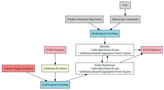
Figure 1.
General flowchart of the methodology for assessing the impact of climate change scenarios on SUDS provision.
The proposed methodology is based on the following key principles.
1. Identify urban boundaries and catchment areas. It is necessary to identify the urban boundaries and the catchment areas in which they are located. This requires the collection of spatial information on urban boundaries and the creation of an elevation model in order to accurately delineate watercourses and their respective catchment areas.
2. Establish the hydrological baseline. To do this, hydrological models need to be developed, parameterised, and supported by relevant data. Our focus is on peak flows and aggregated annual runoff and infiltration values to assess the effectiveness of SUDSs in managing extreme floods and restoring the natural water balance, ensuring runoff to natural watercourses and aquifer recharge through infiltration.
3. Hydrological modelling approach. We used a custom-built conceptual hydrological model based on curve number (CN), developed in Python (version 3.7), for which we required data on catchment land use, precipitation (both daily aggregates and individual storm events), and evapotranspiration.
4. Climate change projections. Information on the projected evolution of weather variables is crucial for evaluating the effectiveness of SUDSs in a changing climate. Understanding how weather variables are expected to change is essential for evaluating the performance of SUDSs in future climate scenarios. To this end, we employed CMIP6 climate projections, focusing particularly on precipitation and surface maximum/minimum temperatures. These data were obtained from the Climate Change Knowledge Portal in the ‘Climate Projections’ section.
The downloaded CSV data were processed to extract the daily mean, maximum, and minimum precipitation and temperature values for all the selected CMIP6 scenarios. In the CMIP6 framework, the transition year between historical simulations and future projections typically occurs around 2015. From this point onwards, climate model projections are driven by a set of standardised scenarios known as shared socio-economic pathways (SSPs), which describe different possible futures based on various levels of socio-economic development, energy use, land use, and greenhouse gas emissions. These SSPs were developed through a comprehensive, community-led process, and are a key component of CMIP6 scenario-based projections [34,35].
Each SSP combines qualitative storylines with quantitative data to characterise future challenges to mitigation and adaptation. For instance, SSP1 depicts a ‘sustainability’ pathway involving minimal challenges to both adaptation and mitigation, whereas SSP5 corresponds to a ‘fossil-fuelled development’ pathway involving significant challenges due to elevated emissions and energy demand. These narratives are supported by sector-specific studies on energy systems [36], land use [37], GHG emission trajectories [38], and air pollution implications [39].
This study incorporates SSP-based projections of precipitation and temperature provided by CMIP6 to simulate future runoff scenarios in urban areas under different potential climate futures.
5. Develop future scenarios for SUDS implementation. Future scenarios for SUDS implementation need to be developed. In our study, we assumed that SUDSs could be represented by variations in the number of representative curves in the catchment area.
We selected the city of Bari (Puglia, Italy) as a case study, as it is a coastal urban area facing specific challenges related to climate and urbanisation. Historical rainfall records were collected to establish baseline conditions, and future projections were integrated to simulate the expected evolution of the hydrological systems. Simulations were conducted under different storm event scenarios using aggregated daily rainfall data.
The following sections outline the details of land use and catchment characterisation (Section 2.1), meteorological data sources and processing (Section 2.2), and the hydrological modelling approach (Section 2.3).
2.1. Identification and Characterisation of Land Use and Catchment Areas
Two main spatial datasets were used for the catchment analysis and modelling of the hydrological system: the digital elevation model (DEM) and land use data.
The DEM data were obtained from the Puglia Territorial Information System (SIT Puglia), and the land use data were obtained from the CORINE Land Cover (CLC) programme, which was developed by the European Environment Agency (EEA) [40].
This spatial information was processed using QGIS (version 3.10). The DEM layer, with its high-resolution topographic information, enabled us to use the GRASS GIS tools r.watershed and r.water.outlet to identify and delineate the catchment boundaries [41].
The r.watershed tool allowed us to define the direction and accumulation of flow within the watershed, and r.water.outlet was used to define the outlet point of each catchment to ensure accurate delineation. Once the catchment boundaries had been defined, the r.mask.rast and r.mask.vect tools were used to trim the CORINE land cover data, ensuring accurate alignment with the vector-based catchment boundaries. This step enabled us to extract land use information relevant to each catchment, facilitating a more accurate characterisation of land use within them.
2.2. Precipitation Data
Weather data with a latency of 30 min were collected from 2010 to August 2024 for the Bari weather station, provided by the Regional Environmental Agency (ARPA PUGLIA). The precipitation records were processed, resulting in 255,608 valid records (Figure 2).
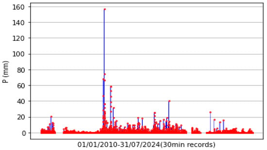
Figure 2.
Recorded 30 min precipitation records in the area of Bari from 2010 to August 2024. Red dots represent individual data points, connected by blue lines.
To simulate the expected evolution over the next 76 years (2025–2100), data from seven common socio-economic pathways (ssp1-1.9, ssp1-2.6, ssp4-3.4, ssp4-2.5, ssp4-6.0, ssp3-7.0, ssp5-8.5) based on the CMIP6 projections were collected. To run the simulations, we grouped the values of all the scenarios and selected the average maximum and minimum values, and Figure 3 shows the results of this process.
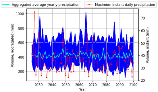
Figure 3.
Aggregated precipitation characteristics from 2025 to 2100. The blue shaded area shows the range of simulated annual precipitation values, while the cyan line represents the ensemble mean. Red dots and lines indicate the maximum daily precipitation recorded each year.
2.3. Hydrology Modelling
In this study, the curve number (CN) method was chosen to simulate the hydrological response of the catchment [42] and running in the hydrological model in Python. The method is based on the concept of a curve number (CN), which represents the combined effect of land use, soil type, and hydrological conditions on runoff potential.
The basic equations used in the CN method are the following:
where:
- E is the runoff depth (in mm);
- P is the precipitation depth (in mm);
- Ia is the initial abstraction (the portion of precipitation that does not contribute to direct runoff, including interception, infiltration, and evaporation);
- S is the potential maximum retention after runoff starts (in mm);
- CN is the curve number, which is a function of land use, hydrological soil group, and cover type.
2.4. Case Study
Puglia is an Italian region located in the south-east of the country, with Bari as its capital (Figure 4). Bari, a coastal city with an area of about 116 km2 and a population of about 315,625, plays a key role in the region, both culturally and economically. The city has a Mediterranean climate with hot, dry summers with temperatures often reaching 30 °C to 35 °C and mild, wet winters with temperatures ranging from 5 °C to 15 °C. Rainfall is concentrated from October to March, with the highest rainfall typically occurring in November, contributing to an annual average of about 500 mm.
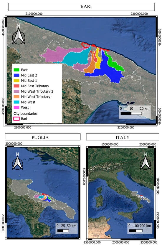
Figure 4.
The figure illustrates the hydrological basins used in the study, which are grouped and colour-coded as follows: East (light green), Mid East 2 (blue), Mid East 1 (yellow), Mid East tributary (red), Mid West tributary 2 (purple), Mid West tributary (orange), Mid West (light blue) and West (pink). The red outline marks the city boundaries of Bari, while the grey outline marks the boundaries of the Puglia region. The composition includes three zoom levels (Italy, Puglia and the Bari basin areas).
3. Results
3.1. Catchment Characterisation
At this stage, the aim was to determine the set of contributing catchments that determine the hydrological cycle in Bari. After generating and analysing different combinations of catchments, it was concluded that a set of eight catchments (Figure 5) are the main determinants of the hydrology in the Bari area.
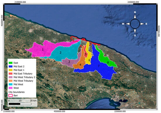
Figure 5.
The basins are numbered and colour-coded as follows: west (1—pink), midwest (2—light blue), midwest tributary 1 (3—purple) and 2 (4—orange), mideast (5—red), mideast tributary 1 (6—yellow), mideast (7—blue), and east (8—green). The red outline marks the city boundaries of Bari.
Once the catchments were determined, the land use information was processed using QGIS (Figure 6) and the CN was assigned to each land use according to the guidelines presented in Table 1, while Table 2 shows the average estimated CN coefficients by catchment.
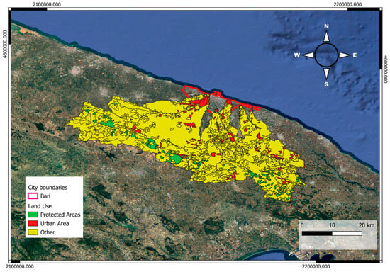
Figure 6.
Catchments’ land use.

Table 1.
Land use groups according to the CORINE Land Cover (CLC) programme [40].

Table 2.
Estimated average curve numbers.
The previous values result in an average curve number of the catchments of 84.01 comprising the catchments in an aggregated area of 159,297.55 km2, with the area of the urban zone in Bari around 120 km2.
3.2. Preprocessing of the Weather Information
The analysis of historical weather data allowed us to establish the baseline in terms of both annual aggregated precipitation and storm events. Figure 7 shows the calculated annual aggregated volumes and statistical distributions of the storm events, while Table 3 summarises the storm characteristics derived from the 30 min rainfall data.
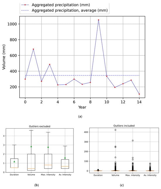
Figure 7.
Aggregated annual precipitation and storm statistical distributions. (a) shows the aggregated annual precipitation (in mm) over the past 14 years. The dashed blue line represents the annual mean. (b) displays boxplots of the characteristics of rainfall events—duration, volume, maximum and average intensity—with outliers excluded. The orange lines represent the medians, while the green triangles indicate the means. (c) shows the same rainfall characteristics, but this time including statistical outliers, which are shown as black circles.

Table 3.
Estimated average curve number (CNs).
To derive representative storm events in each future year, we derived two representative storm events from the historical distributions summarised in Table 3: an extreme storm with a volume of 422 mm and a duration of 2 h (85th quantile of storm duration) and an average storm with a rainfall of 2.84 mm and a duration of 1.18 h. These values were used as a representative baseline. With these values as a representative baseline, we generated a set of two potentially representative storms for each future year (between 2025 and 2100) by simply updating the volumes according to the expected rates of change of the simulated precipitation, i.e., the rates for updating the maximum and average storm events were or
Using these estimated volumes as an average and each annual variance in the data, we randomly generated a set of 1000 storms to simulate the potential evolution of storm events over the years. Table 4 summarises the statistical distributions and Figure 8 the statistical distributions of the two extreme representative scenarios.

Table 4.
Simulation scenarios.
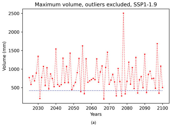
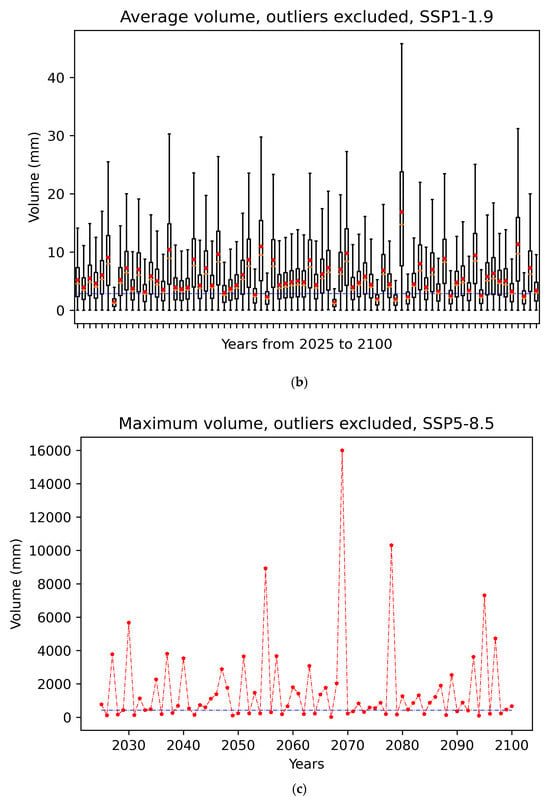
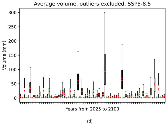
Figure 8.
(a,c) show the maximum rainfall volume per event (in mm) from 2025 to 2100 under the SSP1-1.9 and SSP5-8.5 scenarios, respectively, excluding statistical outliers. Red dots mark annual maxima, connected by dashed red lines. The dashed blue line marks the mean of annual maximum volumes. (b,d) display box plots of average rainfall volumes under the same scenarios. Orange lines show medians and red squares indicate means for each year. The dashed blue line shows the mean of annual average volumes.
Once the simulations had been run, we were able to compare them with the baseline scenario, both in terms of aggregated annual precipitation and individual storm events, as shown in Figure 9.
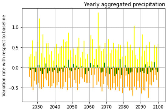
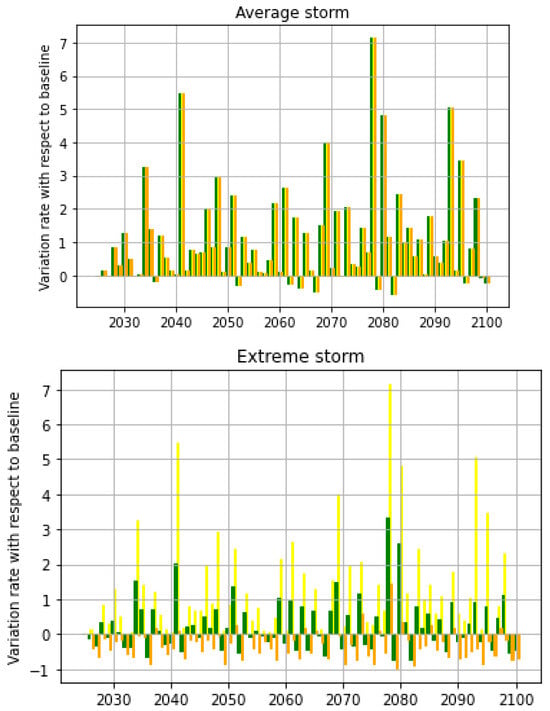
Figure 9.
Rate of change from baseline of annual aggregated precipitation and maximum and average storm events (maximum yellow, average green, minimum orange).
3.3. Results of Hydrological Modelling
Figure 10 shows the results of the hydrological simulations carried out to establish the baseline.
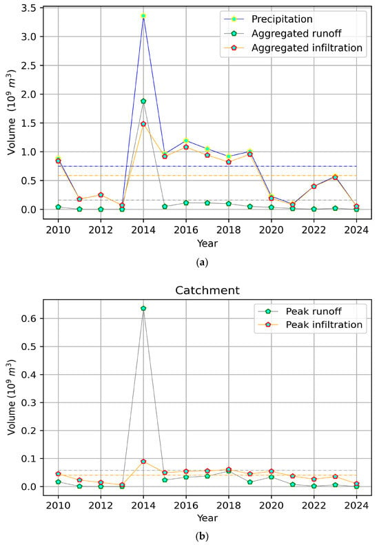
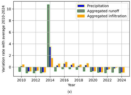
Figure 10.
Baseline hydrological simulations including the set of catchments draining into Bari (dashed lines represent mean values). Annual trends in precipitation, runoff, and infiltration from 2010 to 2024. (a) Aggregated yearly volumes with baseline averages (dashed lines). (b) Peak runoff and infiltration volumes at the catchment scale. (c) Variation rates relative to the baseline average.
Figure 10 shows that the majority of the rainfall infiltrates into the soil, which is consistent with the findings of Bertoldi et al. [43] regarding the infiltration capacity of soils in the region.
Similarly, Figure 11 and Figure 12 show the expected behaviour in the coming years as a result of the hydrological simulations carried out for both the aggregated annual values and the individual storm events, while Figure 13 shows the rates of change with respect to the baseline.
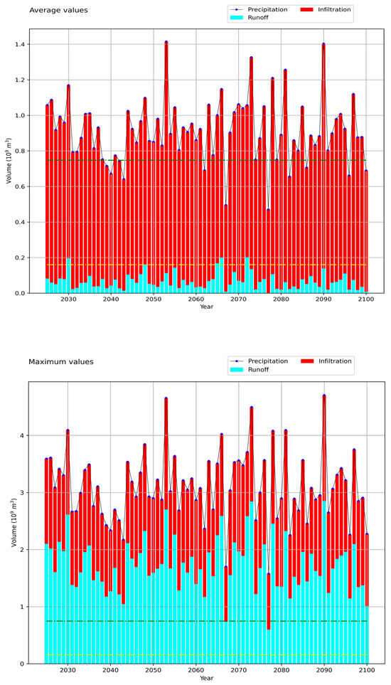
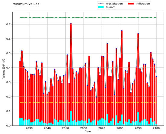
Figure 11.
Simulated expected evolution of precipitation, infiltration and runoff (the dotted lines represent the baseline values of infiltration (green) and runoff (yellow)).
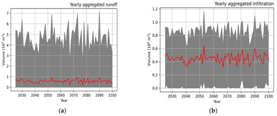
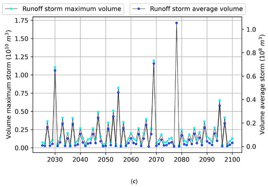
Figure 12.
Expected evolution of infiltration and runoff areas and individual storm events. (a,b) show the projections for the period from 2025 to 2100. The grey shaded areas represent the range of simulated values, and the red lines indicate the mean annual runoff and infiltration rate across the simulations, respectively. (c) shows projected storm runoff volumes for the same period. The cyan line shows the maximum annual storm runoff volume and the blue line shows the average annual storm runoff volume.
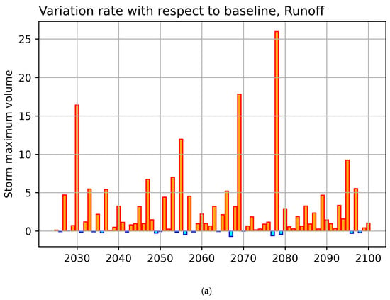
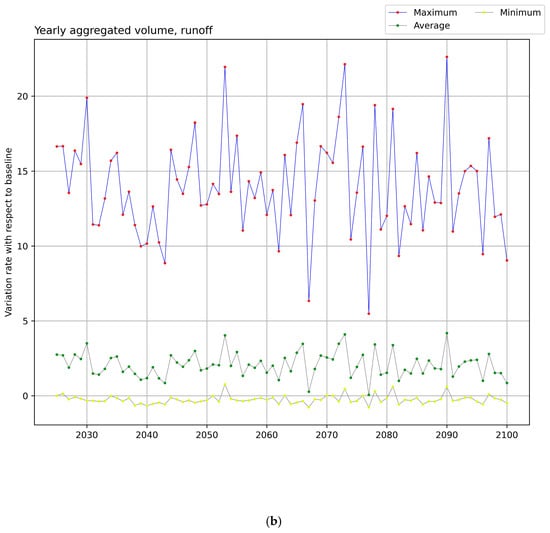
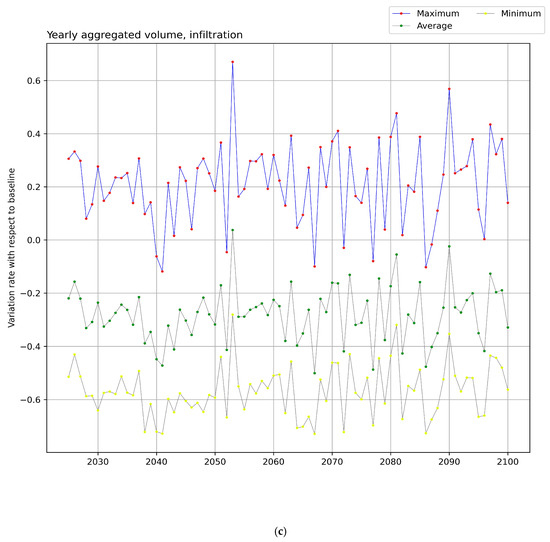
Figure 13.
(a) represents the variation rate of storm runoff volumes relative to the 2010–2024 baseline. The orange bars indicate positive variations (increases), while the blue bars indicate negative variations (decreases). (b,c) show the variation rate of yearly aggregated runoff volumes (maximum-average-minimum) and yearly aggregated infiltration volumes (maximum-average-minimum) from 2025 to 2100, relative to the 2010–2024 baseline, respectively.
The aggregated runoff in Figure 12 shows significant variability, with particularly pronounced peaks in the second half of the century, suggesting an increase in extreme events likely to be driven by climate change. These peaks indicate the risk of severe flooding, putting pressure on water resource management systems. The runoff variation in Figure 13 shows significant fluctuations in maximum values, with peaks reaching 20% above baseline in some years, indicating an increase in the frequency of extreme runoff events. Average values remain more stable, but minimum values are consistently low, suggesting that in some years runoff is minimal.
Given that future urban development and SUDSs implementation will lead to variations in CN, we have simulated the potential evolution of hydrological variables from CN 70 to 99. The results are shown in Figure 14.
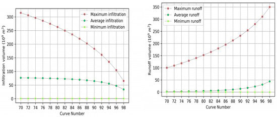
Figure 14.
Potential evolution of maximum, average, and minimum infiltration and runoff (aggregated values over the period 2025–2100) as a function of land use change and potential SUDS implementation expressed by different CN values.
Finally, as an example in contrast to the graphs presented in Figure 11. Figure 15 shows the expected evolution of infiltration and runoff for the maximum, average, and minimum rainfall scenarios for the extreme cases of CN = 70 and CN = 99.
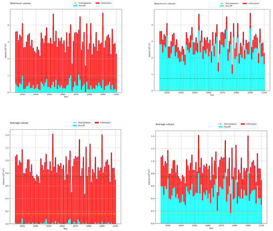
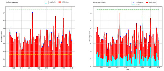
Figure 15.
Evolution of infiltration and runoff for the maximum, average, and minimum precipitation scenarios for the extreme cases of CN = 70 (right column) and CN = 99 (left column). The green dashed line represents the average annual precipitation, while the yellow dashed line shows the average annual runoff relative to the 2010–2024 baseline, respectively.
4. Discussion
In this paper, we present a structured methodology for analysing the potential influence of SUDS implementation at the catchment scale in the context of expected climate change. The methodology aims to provide a comprehensive overview of the evolution of hydrological processes and balances at the catchment scale resulting from different SUDS implementation scenarios. It includes a comprehensive strategy for identifying catchments affected by SUDS implementation, processing territorial and meteorological information, establishing a comparative baseline, and generating simulated scenarios. Currently, there are no established SUDS standards that explicitly address future climate scenarios. Nevertheless, urban planning in the UK and northern Europe increasingly integrates SUDSs as a mitigation strategy, as does urban planning in the USA, China, and Australia [44,45]. However, as Ellis and Lundy have demonstrated, projected increases in runoff under future climate scenarios—particularly under high-emission pathways—may exceed current design thresholds if only minimal climate change allowances (e.g., 20–30%) are applied. This is despite recommendations suggesting allowances of up to 40% to account for more extreme events [46].
Our approach differs from previous ones mainly in terms of spatial scale. While the vast majority of previous studies focus on neighbourhoods or mixed developments (see, for example, references [47,48,49,50,51,52,53,54,55,56]), only a few demonstrate SUDSs at the catchment scale (see references [57,58,59,60,61]). We advocate defining the catchment as the only unit of study. We expect that this approach will provide a more comprehensive view of hydrological systems than focusing on smaller areas. This approach is also more in line with the original SUDS paradigm, which aims to preserve natural dynamics at the catchment scale. The method presented here is not suited to analysing the ability of SUDSs to retain runoff at urban or smaller scales, but rather at catchment scale. Furthermore, in contrast to previous approaches, we compare the effectiveness of SUDSs in maintaining natural hydrological balances against a baseline defined by historical weather data and the actual distribution of land use. In the example presented in this paper, we used actual urban land use rather than the potential state of the catchment prior to urbanisation. This scenario can easily be included in the method by defining land use in the absence of urban development such that the baseline refers to this situation, enabling the SUDS effect to be targeted to restore the original conditions in the context of climate change. Existing studies on the effectiveness of SUDSs typically do not define a baseline for comparison, instead analysing the effect of SUDSs in absolute terms.
For example, Marko et al. [62] merely examine the absolute reduction in peak flows, reporting values ranging from 23% to 97%. However, they neither establish a reference hydrological condition nor consider how these reductions compare with pre-urbanisation runoff patterns. Few studies focus on assessing the ability to restore natural hydrological conditions rather than simply comparing the effectiveness of different SUDS configurations [63,64]. We assume that the natural balance must be maintained at catchment scale, initially in terms of runoff and infiltration (aquifer recharge).
While many civil engineering approaches focus on small-scale interventions within urban environments, driven by infrastructure-specific performance metrics [65], hydrologists must adopt a broader, system-based perspective. The catchment area must be considered an interconnected, dynamic network of interacting components. Localised or isolated interventions may fail to address hydrological imbalances across the entire system. In this context, SUDSs should be evaluated not only for their localised effects but also for their ability to restore and maintain natural hydrological equilibrium at catchment level.
Previous studies have highlighted the need to understand the impact of specific aspects on SUDS performance, such as spatial distribution and timescales [26].
Recent studies have incorporated individual future scenarios to simulate SUDS performance (see, for example, Chen, C.L. [66]).
However, these studies have only been applied to specific case studies, failing to propose a standardised methodology to address these gaps. Motivated by these gaps, this paper presents a structured methodology for analysing the potential influence of SUDS implementation at catchment scale in an evolving climate. Pooling data and analysing the range between maximum and minimum values provides a more meaningful understanding of SUDS effectiveness. In this study, we adopted the curve number (CN) method because we believe that its simple parameterisation will facilitate the practical application of the proposed methodology, particularly in urban contexts. Note that this method was developed in 1954 by the US Department of Agriculture’s Soil Conservation Service (SCS) [42]. Historically, many authors have highlighted limitations, such as its design for single-event simulations and small to medium-sized catchments. Additionally, it does not account for complex hydrological processes such as subsurface flow, intra-storm rainfall variability, or dynamically changing soil moisture. Furthermore, assumptions such as fixed initial abstraction and sensitivity to land use and antecedent moisture conditions can introduce uncertainties, particularly in diverse, densely populated urban areas [67,68,69].
A wide range of rainfall–runoff models have been developed worldwide. Each model is designed to meet specific hydrological objectives, spatial resolutions, and constraints on data availability. These models can be broadly grouped into four categories: empirical, conceptual, physically based, and data-driven approaches [70,71,72].
- Empirical models, such as the rational method, the Horton infiltration model [73], the curve number method [74], the Green–Ampt method [75], and ACRU [76], rely on simplified relationships derived from observed data. While these models are easy to implement and interpret, they may lack robustness when transferred to catchments with varying physical characteristics.
- Physically based models, including SHE [77], SWAT [78], and IHDM [79], attempt to simulate hydrological processes through governing equations of mass and momentum conservation. These models allow for fine-resolution process representation, but demand extensive, high-quality input data (e.g., soil hydraulic properties and detailed DEMs) and significant computational resources, which often limits their applicability in small urban catchments or regions with limited data [80].
- Conceptual models, such as the HBV model [81], the GR4J model [82], and the Stanford watershed model [83], conceptualise catchments using simplified storage and flow components. They balance physical realism and operational simplicity, but generally require careful calibration and may be sensitive to input uncertainty.
- Data-driven models, particularly those using machine learning (ML) or deep learning (DL) techniques, are being used more and more in hydrology [84]. These models can learn complex nonlinear relationships from data without requiring explicit physical equations. However, their reliance on long-term historical data and limited interpretability restrict their use in regulatory and planning contexts [85].
Despite its conceptual simplicity, the curve number (CN) method remains one of the most effective and widely adopted techniques for estimating surface runoff [86]. Its main advantage is its ability to combine key factors that generate runoff—land use, soil type, and antecedent moisture conditions—into a single, empirically derived parameter. These inputs are often available in standardised forms, such as GIS-based land cover maps and urban planning documentation, making the method suitable for rapid assessments, preliminary designs, and decision-making in settings with limited data [87].
In line with Moradkhani and Sorooshian’s principle [88], which defines an optimal model as one that yields realistic results with minimal complexity and few parameters, the CN method offers a pragmatic solution. Although it is currently widely used for urban hydrology and stormwater management, it was originally developed for use in agricultural catchments [89]. This origin highlights its suitability for broader catchment-scale hydrological analysis, where diverse land cover, soil properties, and spatial variability interact.
However, the method’s broader analytical potential has increasingly been overshadowed by its dominant application in localised or urbanised contexts. This study aimed to reposition the CN method, presenting it not merely as a simplified urban runoff estimator, but as a practical, scalable, and adaptable tool for evaluating the hydrological response across entire catchments under current and future climate scenarios.
Having explained the reason for choosing the CN number model, we finally incorporated SUDS scenarios into the model by adjusting the catchment’s average curve number, as per Rohman et al. [90]. This simplifies model operation and scenario generation. As previously discussed, this approach does not allow for the local analysis of factors such as peak flow generation or attenuation. However, it provides a broader perspective on the impact on aggregated catchment processes.
The discussion, then, moves on to the need for greater consideration of scale, focusing on the catchment as a whole to ensure a more holistic approach to managing hydrological resources. Another important example comes from the study by D’Ambrosio et al. [91], which analysed the effectiveness of SUDSs in an Italian urban context. The study showed that retrofitting SUDSs across approximately 8.3% of the study area significantly reduced total runoff and peak flows. Additionally, the proportion of nodes in the urban network in critical condition decreased from 52% to 24%. Finally, the paper by Chapman et al. [92] emphasised the importance of extensive SUDS implementation to reduce peak flows. Their study found that the scenario with the highest level of SUDS implementation (using a combination of infiltration and storage) produced the lowest peak flows, thus helping to limit the impact of heavy rainfall. Finally, building on the foundations of the previous study, we explored how SUDSs can be represented using the CN approach. To date, only one study appears to come close to our proposed approach. A recent study by Huq et al. [93] presents a climate-resilient urban drainage model based on GIS and the SCS-CN method, and demonstrates its efficiency in ten summary points. While our approach is highly comparable to this existing study, a key limitation is the lack of analysis of future land use change (LULC), which could affect the long-term effectiveness of our model. Despite this, no other study appears to have proposed a similar methodology to ours for SUDS applications, highlighting the innovative nature of our model. We strongly recommend that future SUDS design phases be carried out using high-resolution, site-specific hydrological and hydraulic models. These models should consider the interactions between urban surface and subsurface drainage systems and natural watercourses to ensure a more complete and accurate assessment. Finally, we suggest that representing SUDS treatment trains—integrating multiple types of SUDSs to improve overall system performance—is a highly effective strategy [94]. In conclusion, while a significant body of literature emphasises the importance of SUDSs, there is still a substantial administrative and legislative gap at a practical level. This limited perspective is reflected in current policies. SUDSs are mandatory only in specific regions, such as Wales in the UK, Singapore under the ABC Waters Programme, and selected US cities, including Philadelphia, Portland, and Seattle, under MS4-permitting systems. They are also mandatory in Denmark and a few other countries. In light of our findings, we endorse Ellis and Lundy’s recommendation [44] to increase design allowances by up to 40% to ensure performance under more extreme future rainfall events. This reinforces the necessity of adapting SUDS design standards to evolving climate scenarios.
5. Conclusions
This study presents a structured methodology for evaluating the impact of SUDS implementation at catchment level in an evolving climate. This approach was found to be effective and applicable in a real-world context, as demonstrated by the Bari, Italy case study. This methodology can be applied to any small to medium-sized urban catchment area regardless of climate conditions, provided basic data on land use and precipitation are available.
To support climate-resilient urban drainage planning, digital elevation models (DEMs) were integrated with a GIS-based application of the SCS-CN method. Using the curve number approach, the simulation estimates runoff volumes under various climate and land use scenarios. The key step was to compare these volumes with a historical baseline, which made it possible to quantify the storage capacity required to restore or maintain the area’s natural hydrological balance. This insight can then be used to estimate the type and number of SUDS elements needed across different urban catchments, tailored to future climate projections.
The results show that extreme storm volumes could increase 7-fold, while average storm volumes could increase 2.5-fold. This would pose a significant challenge to the current capacity of drainage infrastructure. Additionally, discharge peaks could exceed baseline values by up to 20% in some years, indicating a greater occurrence of extreme runoff events. Taken together, these findings suggest an increased risk of both flash floods and prolonged droughts in future decades, a risk that is further exacerbated by ongoing urbanisation.
Based on these findings, we recommend:
- In practice: Prioritising the widespread implementation of SUDSs at the catchment scale, especially in areas undergoing intense urban development.
- Policy: Updating regulatory frameworks to assess SUDS performance based on their ability to restore natural hydrological balances, not just reduce peak flows.
- Research: Future land use changes must be integrated and the demand for SUDSs estimated to support decision-making.
- Resilience: Adopting scenario-based methodologies to improve long-term planning in the face of climate uncertainty, such as the one proposed.
This methodology provides a strategic foundation to support sustainable urban water management and can be adapted to different territorial and climatic contexts.
Author Contributions
Conceptualization, S.Z., A.P.M. and M.T.G.-V.; methodology, S.Z., A.P.M. and M.T.G.-V.; validation, S.Z., A.P.M. and M.T.G.-V.; formal analysis, S.Z., A.P.M. and M.T.G.-V.; investigation, S.Z., A.P.M., R.S.V. and M.T.G.-V.; data curation, S.Z., A.P.M., R.S.V. and M.T.G.-V.; writing—original draft preparation, S.Z., A.P.M. and M.T.G.-V.; writing—review and editing, S.Z., A.P.M. and M.T.G.-V.; visualization, S.Z., A.P.M., R.S.V. and M.T.G.-V.; supervision, S.Z., A.P.M. and M.T.G.-V. All authors have read and agreed to the published version of the manuscript.
Funding
This research project has been funded by the Comunidad de Madrid through the call Research Grants for Young Investigators from the Universidad Politécnica de Madrid.
Institutional Review Board Statement
Not applicable.
Informed Consent Statement
Not applicable.
Data Availability Statement
Data sharing is not applicable to this article as no datasets were generated or analyzed during the study.
Conflicts of Interest
The authors declare no conflict of interest.
References
- Jia, M.; Lin, J.; Dai, J.; Zhang, J. Assessing future flood risks in megacity suburbs under shared socioeconomic pathways (SSPs) scenarios: A case study of Beijing. Urban Clim. 2024, 58, 102208. [Google Scholar] [CrossRef]
- Chen, S.S.; Tsang, D.C.; He, M.; Sun, Y.; Lau, L.S.; Leung, R.W.; Lau, E.S.; Hou, D.; Liu, A.; Mohanty, S. Designing sustainable drainage systems in subtropical cities: Challenges and opportunities. J. Clean. Prod. 2021, 280, 124418. [Google Scholar] [CrossRef]
- Kõiv-Vainik, M.; Kill, K.; Espenberg, M.; Uuemaa, E.; Teemusk, A.; Maddison, M.; Palta, M.M.; Török, L.; Mander, Ü.; Scholz, M.; et al. Urban stormwater retention capacity of nature-based solutions at different climatic conditions. Nat.-Based Solut. 2022, 2, 100038. [Google Scholar] [CrossRef]
- Ferrans, P.; Torres, M.N.; Temprano, J.; Sánchez, J.P.R. Sustainable Urban Drainage System (SUDS) modeling supporting decision-making: A systematic quantitative review. Sci. Total Environ. 2022, 806, 150447. [Google Scholar] [CrossRef]
- Monteiro, C.M.; Mendes, A.M.; Santos, C. Green roofs as an urban NbS strategy for rainwater retention: Influencing factors—A review. Water 2023, 15, 2787. [Google Scholar] [CrossRef]
- Monachese, A.P.; Gómez-Villarino, M.T.; López-Santiago, J.; Sanz, E.; Almeida-Ñauñay, A.F.; Zubelzu, S. Challenges and Innovations in Urban Drainage Systems: Sustainable Drainage Systems Focus. Water 2024, 17, 76. [Google Scholar] [CrossRef]
- Alsubih, M.; Arthur, S.; Wright, G.; Allen, D. Experimental study on the hydrological performance of a permeable pavement. Urban Water J. 2017, 14, 427–434. [Google Scholar] [CrossRef]
- Rodríguez-Rojas, M.I.; Huertas-Fernández, F.; Moreno, B.; Martínez, G.; Grindlay, A.L. A study of the application of permeable pavements as a sustainable technique for the mitigation of soil sealing in cities: A case study in the south of Spain. J. Environ. Manag. 2018, 205, 151–162. [Google Scholar] [CrossRef]
- Tota-Maharaj, K.; Hills, C.D.; Staddon, C.; Monrose, J. Enhancing the ecological ability of Permeable Pavements Systems (PPS) as urban stormwater Green infrastructure. J. Assoc. Prof. Eng. Trinidad Tobago 2024, 52, 4–16. [Google Scholar]
- Huang, P.; Zhang, K.; Chui, T.F.M. Hydrologic performance of permeable pavements under extreme and regular rainfall conditions. J. Hydrol. 2025, 652, 132653. [Google Scholar] [CrossRef]
- Cipolla, S.S.; Maglionico, M.; Stojkov, I. A long-term hydrological modelling of an extensive green roof by means of SWMM. Ecol. Eng. 2016, 95, 876–887. [Google Scholar] [CrossRef]
- Andrés-Doménech, I.; Perales-Momparler, S.; Morales-Torres, A.; Escuder-Bueno, I. Hydrological performance of green roofs at building and city scales under Mediterranean conditions. Sustainability 2018, 10, 3105. [Google Scholar] [CrossRef]
- Alim, M.A.; Rahman, A.; Tao, Z.; Garner, B.; Griffith, R.; Liebman, M. Green roof as an effective tool for sustainable urban development: An Australian perspective in relation to stormwater and building energy management. J. Clean. Prod. 2022, 362, 132561. [Google Scholar] [CrossRef]
- Gullotta, A.; Musmeci, F.; Cancelliere, A.; Campisano, A. Comparing potential for storm water control of different full-scale blue roofs by field experiments. Urban Water J. 2025, 22, 200–209. [Google Scholar] [CrossRef]
- Orsi, E.; Crispino, G.; Iervolino, M.; Gisonni, C. Hydraulic and Hydrologic Invariance: Effectiveness of Green Roofs and Permeable Pavements. J. Irrig. Drain. Eng. 2025, 151, 04025001. [Google Scholar] [CrossRef]
- McLeod, M.K.; Mickovski, S.B. The use of end-of-line SUDS for residential development. J. Sustain. Res. 2024, 6, e240031. [Google Scholar]
- Lhamidi, K.; El Khattabi, J.; Nguyen, H.D.; Aljer, A. Hydrological Performance Assessment of Low-Impact Development Practices: A Vegetated Swale Case Study. Water 2024, 16, 2018. [Google Scholar] [CrossRef]
- Wang, M.; Zhuang, J.A.; Sun, C.; Wang, L.; Zhang, M.; Fan, C.; Li, J. The Application of Rain Gardens in Urban Environments: A Bibliometric Review. Land 2024, 13, 1702. [Google Scholar] [CrossRef]
- Tobio, J.A.S.; Maniquiz-Redillas, M.C.; Kim, L.H. Physical design optimization of an urban runoff treatment system using Stormwater Management Model (SWMM). Water Sci. Technol. 2015, 72, 1747–1753. [Google Scholar] [CrossRef]
- Baek, S.-S.; Ligaray, M.; Pyo, J.; Park, J.-P.; Kang, J.-H.; Pachepsky, Y.; Chun, J.A.; Cho, K.H. A novel water quality module of the SWMM model for assessing low impact development (LID) in urban watersheds. J. Hydrol. 2020, 586, 124886. [Google Scholar] [CrossRef]
- Kourtis, I.M.; Bellos, V.; Kopsiaftis, G.; Psiloglou, B.; Tsihrintzis, V.A. Methodology for holistic assessment of grey-green flood mitigation measures for climate change adaptation in urban basins. J. Hydrol. 2021, 603, 126885. [Google Scholar] [CrossRef]
- Rosa, D.J.; Clausen, J.C.; Dietz, M.E. Calibration and verification of SWMM for low impact development. JAWRA J. Am. Water Resour. Assoc. 2015, 51, 746–757. [Google Scholar] [CrossRef]
- Kourtis, I.M.; Tsihrintzis, V.A.; Baltas, E. Simulation of low impact development (LID) practices and comparison with conventional drainage solutions. Proceedings 2018, 2, 640. [Google Scholar] [CrossRef]
- Peker, İ.B.; Gülbaz, S. Impact of rapid anthropogenic land use and land cover change on basin hydrology and sediment loads. Landsc. Ecol. Eng. 2025, 21, 65–79. [Google Scholar] [CrossRef]
- Maftuhah, D.I.; Anityasari, M.; Sholihah, M. Model of urban water management towards water sensitive city: A literature review. IOP Conf. Ser. Mater. Sci. Eng. 2018, 337, 012047. [Google Scholar] [CrossRef]
- Bai, Y.; Zhao, N.; Zhang, R.; Zeng, X. Storm water management of low impact development in urban areas based on SWMM. Water 2018, 11, 33. [Google Scholar] [CrossRef]
- Rujner, H.; Leonhardt, G.; Marsalek, J.; Viklander, M. High-resolution modelling of the grass swale response to runoff inflows with Mike SHE. J. Hydrol. 2018, 562, 411–422. [Google Scholar] [CrossRef]
- Garbanzos, S.; Maniquiz-Redillas, M. Modeling the hydrologic performance and cost-effectiveness of LID in a residential park area using a decentralized design approach. Hydrology 2022, 9, 62. [Google Scholar] [CrossRef]
- Arjenaki, M.O.; Sanayei, H.R.Z.; Heidarzadeh, H.; Mahabadi, N.A. Modeling and investigating the effect of the LID methods on collection network of urban runoff using the SWMM model (case study: Shahrekord City). Model. Earth Syst. Environ. 2021, 7, 1–16. [Google Scholar] [CrossRef]
- Zhu, Z.; Chen, Z.; Chen, X.; Yu, G. An assessment of the hydrologic effectiveness of low impact development (LID) practices for managing runoff with different objectives. J. Environ. Manag. 2019, 231, 504–514. [Google Scholar] [CrossRef]
- Macro, K.; Matott, L.S.; Rabideau, A.; Ghodsi, S.H.; Zhu, Z. OSTRICH-SWMM: A new multi-objective optimization tool for green infrastructure planning with SWMM. Environ. Model. Softw. 2019, 113, 42–47. [Google Scholar] [CrossRef]
- Ma, Y.; Xia, X.; Liang, Q.; Wan, H. Investigating the Impact of Spatial Distribution of Sustainable Drainage System (SuDS) Components on Their Flood Mitigation Performance in Communities with High Groundwater Levels. Water 2022, 14, 1367. [Google Scholar] [CrossRef]
- Kourtis, I.M.; Tsihrintzis, V.A.; Baltas, E. A robust approach for comparing conventional and sustainable flood mitigation measures in urban basins. J. Environ. Manag. 2020, 269, 110822. [Google Scholar] [CrossRef]
- O’Neill, B.C.; Oppenheimer, M.; Warren, R.; Hallegatte, S.; Kopp, R.E.; Pörtner, H.O.; Scholes, R.; Birkmann, J.; Foden, W.; Licker, R.; et al. IPCC reasons for concern regarding climate change risks. Nat. Clim. Change 2017, 7, 28–37. [Google Scholar] [CrossRef]
- Turnock, S.T.; Allen, R.J.; Andrews, M.; Bauer, S.E.; Deushi, M.; Emmons, L.; Good, P.; Horowitz, L.; John, J.G.; Michou, M.; et al. Historical and future changes in air pollutants from CMIP6 models. Atmos. Chem. Phys. 2020, 20, 14547–14579. [Google Scholar] [CrossRef]
- Bauer, N.; Calvin, K.; Emmerling, J.; Fricko, O.; Fujimori, S.; Hilaire, J.; Eom, J.; Krey, V.; Kriegler, E.; Mouratiadou, I.; et al. Shared socio-economic pathways of the energy sector–quantifying the narratives. Glob. Environ. Change 2017, 42, 316–330. [Google Scholar] [CrossRef]
- Popp, A.; Calvin, K.; Fujimori, S.; Havlik, P.; Humpenöder, F.; Stehfest, E.; Bodirsky, B.L.; Dietrich, J.P.; Doelmann, J.C.; Gusti, M.; et al. Land-use futures in the shared socio-economic pathways. Glob. Environ. Change 2017, 42, 331–345. [Google Scholar] [CrossRef]
- Riahi, K.; Rao, S.; Krey, V.; Cho, C.; Chirkov, V.; Fischer, G.; Kindermann, G.; Nakicenovic, N.; Rafaj, P. RCP 8.5—A scenario of comparatively high greenhouse gas emissions. Clim. Change 2011, 109, 33–57. [Google Scholar] [CrossRef]
- Rao, S.; Klimont, Z.; Smith, S.J.; Van Dingenen, R.; Dentener, F.; Bouwman, L.; Riahi, K.; Amann, M.; Bodirsky, B.L.; van Vuuren, D.P.; et al. Future air pollution in the Shared Socio-economic Pathways. Glob. Environ. Change 2017, 42, 346–358. [Google Scholar] [CrossRef]
- Cover, C.L. Copernicus Land Monitoring Service; European Environment Agency (EEA): Copenhagen, Denmark, 2018. [Google Scholar]
- Schwartze, C. Deriving hydrological response units (HRUs) using a web processing service implementation based on GRASS GIS. Geoinform. FCE CTU 2008, 3, 67–78. [Google Scholar] [CrossRef]
- Mishra, S.K.; Pandey, A.; Singh, V.P. Special issue on soil conservation service curve number (SCS-CN) methodology. J. Hydrol. Eng. 2012, 17, 1157. [Google Scholar] [CrossRef]
- Bertoldi, G.; Notarnicola, C.; Brenner, J.; Greifeneder, F.; Castelli, M.; Niedrist, G.; Tappeiner, U. Modelling Feedbacks between Vegetation and Soil Moisture in Mountain Grasslands. In Proceedings of the XXI CMWR Conference, Toronto, ON, Canada, 20–24 June 2016. [Google Scholar]
- Lashford, C.; Rubinato, M.; Cai, Y.; Hou, J.; Abolfathi, S.; Coupe, S.; Charlesworth, S.; Tait, S. SuDS & sponge cities: A comparative analysis of the implementation of pluvial flood management in the UK and China. Sustainability 2019, 11, 213. [Google Scholar] [CrossRef]
- Charlesworth, S.M.; Harkerand, E.; Rickard, S. A Review of Sustainable Drainage Systems (SuDS) A Soft Option for Hard Drainage Questions? Geography 2003, 88, 99–107. [Google Scholar] [CrossRef]
- Ellis, J.B.; Lundy, L. Implementing sustainable drainage systems for urban surface water management within the regulatory framework in England and Wales. J. Environ. Manag. 2016, 183, 630–636. [Google Scholar] [CrossRef]
- Haghighatafshar, S.; Yamanee-Nolin, M.; Larson, M. A physically based model for mesoscale SuDS—An alternative to large-scale urban drainage simulations. J. Environ. Manag. 2019, 240, 527–536. [Google Scholar] [CrossRef] [PubMed]
- Cotterill, S.; Bracken, L.J. Assessing the effectiveness of sustainable drainage systems (SuDS): Interventions, impacts and challenges. Water 2020, 12, 3160. [Google Scholar] [CrossRef]
- Nóblega Carriquiry, A.; Sauri, D.; March, H. Community involvement in the implementation of sustainable urban drainage systems (SUDSs): The case of Bon Pastor, Barcelona. Sustainability 2020, 12, 510. [Google Scholar] [CrossRef]
- Thodesen, B.; Time, B.; Kvande, T. Sustainable Urban Drainage Systems: Themes of Public Perception—A Case Study. Land 2022, 11, 589. [Google Scholar] [CrossRef]
- Guptha, G.C.; Swain, S.; Al-Ansari, N.; Taloor, A.K.; Dayal, D. Assessing the role of SuDS in resilience enhancement of urban drainage system: A case study of Gurugram City, India. Urban Clim. 2022, 41, 101075. [Google Scholar] [CrossRef]
- Jiménez Ariza, S.L.; Martínez, J.A.; Muñoz, A.F.; Quijano, J.P.; Rodríguez, J.P.; Camacho, L.A.; Díaz-Granados, M. A multicriteria planning framework to locate and select sustainable urban drainage systems (SUDS) in consolidated urban areas. Sustainability 2019, 11, 2312. [Google Scholar] [CrossRef]
- Vollaers, V.; Nieuwenhuis, E.; van de Ven, F.; Langeveld, J. Root causes of failures in sustainable urban drainage systems (SUDS): An exploratory study in 11 municipalities in The Netherlands. Blue-Green Syst. 2021, 3, 31–48. [Google Scholar] [CrossRef]
- Suárez-Inclán, A.M.; Allende-Prieto, C.; Roces-García, J.; Rodríguez-Sánchez, J.P.; Sañudo-Fontaneda, L.A.; Rey-Mahía, C.; Álvarez-Rabanal, F.P. Development of a Multicriteria Scheme for the Identification of Strategic Areas for SUDS Implementation: A Case Study from Gijón, Spain. Sustainability 2022, 14, 2877. [Google Scholar] [CrossRef]
- Ho, H.L.; Babel, M.S.; Weesakul, S.; Irvine, K.N.; Pham, M.D. Exploratory assessment of SUDS feasibility in Nhieu Loc-Thi Nghe Basin, Ho Chi Minh City, Vietnam. Br. J. Environ. Clim. Change 2015, 5, 91–103. [Google Scholar]
- Jato-Espino, D.; Charlesworth, S.M.; Bayon, J.R.; Warwick, F. Rainfall–runoff simulations to assess the potential of SuDS for mitigating flooding in highly urbanized catchments. Int. J. Environ. Res. Public Health 2016, 13, 149. [Google Scholar] [CrossRef]
- Binesh, N.; Niksokhan, M.H.; Sarang, A.; Rauch, W. Improving sustainability of urban drainage systems for climate change adaptation using best management practices: A case study of Tehran, Iran. Hydrol. Sci. J. 2019, 64, 381–404. [Google Scholar] [CrossRef]
- Zubelzu, S.; Rodríguez-Sinobas, L.; Sordo-Ward, A.; Pérez-Durán, A.; Cisneros-Almazán, R. Multi-objective approach for determining optimal sustainable urban drainage systems combination at city scale. the case of San Luis Potosí (México). Water 2020, 12, 835. [Google Scholar] [CrossRef]
- D’Ambrosio, R.; Longobardi, A.; Schmalz, B. SuDS as a climate change adaptation strategy: Scenario-based analysis for an urban catchment in northern Italy. Urban Clim. 2023, 51, 101596. [Google Scholar] [CrossRef]
- Marko, I.; Wittmanová, R.; Hrudka, J.; Stanko, Š. The effectiveness of SuDS measures in reducing the rainwater runoff from urbanized areas. IOP Conf. Ser. Mater. Sci. Eng. 2021, 1209, 012021. [Google Scholar] [CrossRef]
- Kim, H.W.; Park, Y. Urban green infrastructure and local flooding: The impact of landscape patterns on peak runoff in four Texas MSAs. Appl. Geogr. 2016, 77, 72–81. [Google Scholar] [CrossRef]
- Haghighatafshar, S.; la Cour Jansen, J.; Aspegren, H.; Jönsson, K. Conceptualization and schematization of mesoscale sustainable drainage systems: A full-scale study. Water 2018, 10, 1041. [Google Scholar] [CrossRef]
- Qiu, H.; Wu, K.; Ayasrah, M.M.; Huang, W. Study on Sunlight Temperature Field of Steel Box Arch Ribs in Irregular Arch Bridges. Symmetry 2024, 16, 413. [Google Scholar] [CrossRef]
- Guo, X.; Feng, C.; Gu, E.; Tian, C.; Shen, Z. Spatial distribution, source apportionment and risk assessment of antibiotics in the surface water and sediments of the Yangtze Estuary. Sci. Total Environ. 2019, 671, 548–557. [Google Scholar] [CrossRef]
- Abduljaleel, Y.; Demissie, Y. Identifying cost-effective low-impact development (LID) under climate change: A multi-objective optimization approach. Water 2022, 14, 3017. [Google Scholar] [CrossRef]
- Chen, C.L. An evaluation of the mathematics and physical significance of the soil conservation service curve number procedure for estimating runoff volume. In Proceedings of the International Symposium on Rainfall-Runoff Modeling; Water Resources Publications: Littleton, CO, USA, 1982; pp. 387–418. [Google Scholar]
- Bales, J.; Betson, R.P. The curve number as a hydrologic index. In Rainfall Runoff Relationship; Singh, V.P., Ed.; Water Resources Publication: Littleton, CO, USA, 1981; pp. 371–386. [Google Scholar]
- Ponce, V.M.; Hawkins, R.H. Runoff curve number: Has it reached maturity? J. Hydrol. Eng. 1996, 1, 11–19. [Google Scholar] [CrossRef]
- Mishra, S.K.; Suresh Babu, P.; Singh, V.P. SCS-CN method revisited. In Advances in Hydraulics and Hydrology; Water Resources Publications: Littleton, CO, USA, 2007. [Google Scholar]
- Jehanzaib, M.; Ajmal, M.; Achite, M.; Kim, T.W. Comprehensive review: Advancements in rainfall-runoff modelling for flood mitigation. Climate 2022, 10, 147. [Google Scholar] [CrossRef]
- Pandi, D.; Kothandaraman, S.; Kuppusamy, M. Hydrological models: A review. Int. J. Hydrol. Sci. Technol. 2021, 12, 223–242. [Google Scholar] [CrossRef]
- Devia, G.K.; Ganasri, B.P.; Dwarakish, G.S. A review on hydrological models. Aquat. Procedia 2015, 4, 1001–1007. [Google Scholar] [CrossRef]
- Thompson, D.B. The Rational Method, Regional Regression Equations, and Site-Specific Flood-Frequency Relations; No. FHWA/TX–06/0-4405-1; Texas Tech University, Center for Multidisciplinary Research in Transportation: Broadway Lubbock, TX, USA, 2006. [Google Scholar]
- Beven, K.; Robert, E. Horton’s perceptual model of infiltration processes. Hydrol. Process. 2004, 18, 3447–3460. [Google Scholar] [CrossRef]
- Ali, S.; Islam, A.; Mishra, P.K.; Sikka, A.K. Green-Ampt approximations: A comprehensive analysis. J. Hydrol. 2016, 535, 340–355. [Google Scholar] [CrossRef]
- Warburton, M.L.; Schulze, R.E.; Jewitt, G.P. Confirmation of ACRU model results for applications in land use and climate change studies. Hydrol. Earth Syst. Sci. 2010, 14, 2399–2414. [Google Scholar] [CrossRef]
- Im, S.; Kim, H.; Kim, C.; Jang, C. Assessing the impacts of land use changes on watershed hydrology using MIKE SHE. Environ. Geol. 2009, 57, 231–239. [Google Scholar] [CrossRef]
- Arnold, J.G.; Moriasi, D.N.; Gassman, P.W.; Abbaspour, K.C.; White, M.J.; Srinivasan, R.; Santhi, C.; Harmel, R.D.; van Griensven, A.; Van Liew, M.W.; et al. SWAT: Model use, calibration, and validation. Trans. ASABE 2012, 55, 1491–1508. [Google Scholar] [CrossRef]
- Calver, A.; Wood, W.L. The Institute of Hydrology Distributed Model; Institute of Hydrology: Wallingford, UK, 1995; pp. 595–626. [Google Scholar]
- Paniconi, C.; Putti, M. Physically based modeling in catchment hydrology at 50: Survey and outlook. Water Resour. Res. 2015, 51, 7090–7129. [Google Scholar] [CrossRef]
- Seibert, J.; Bergström, S. A retrospective on hydrological catchment modelling based on half a century with the HBV model. Hydrol. Earth Syst. Sci. 2022, 26, 1371–1388. [Google Scholar] [CrossRef]
- Hublart, P.; Ruelland, D.; Garcĺa De Cortázar Atauri, I.; Ibacache, A. Reliability of a conceptual hydrological model in a semi-arid Andean catchment facing water-use changes. Proc. Int. Assoc. Hydrol. Sci. 2015, 371, 203–209. [Google Scholar] [CrossRef]
- Donigian, A.S.; Imhoff, J. History and evolution of watershed modeling derived from the Stanford Watershed Model. In Watershed Models; CRC Press: Boca Raton, FL, USA, 2006; pp. 21–45. [Google Scholar]
- Remesan, R.; Mathew, J. Hydrological data driven modelling. In Earth System Data and Models; Springer: New York, NY, USA, 2015; p. 1. [Google Scholar]
- Oyebode, O.K.; Otieno, F.A.O.; Adeyemo, J. Review of three data-driven modelling techniques for hydrological modelling and forecasting. Fresenius Environ. Bull. 2014, 23, 1443–1454. [Google Scholar]
- Lal, M.; Mishra, S.K.; Pandey, A. Physical verification of the effect of land features and antecedent moisture on runoff curve number. Catena 2015, 133, 318–327. [Google Scholar] [CrossRef]
- Mishra, S.K.; Singh, V.P. Soil Conservation Service Curve Number (SCS-CN) Methodology; Springer Science & Business Media: Berlin/Heidelberg, Germany, 2013; Volume 42. [Google Scholar]
- Moradkhani, H.; Sorooshian, S. General Review of Rainfall-Runoff Modeling: Model Calibration, Data Assimilation, and Uncertainty Analysi; Springer: Berlin/Heidelberg, Germany, 2008; pp. 1–24. [Google Scholar]
- Soulis, K.X. Soil conservation service curve number (SCS-CN) Method: Current applications, remaining challenges, and future perspectives. Water 2021, 13, 192. [Google Scholar] [CrossRef]
- Rohman, A.; Comber, A.; Mitchell, G. Evaluation of natural flood management using curve number in the Ciliwung Basin, West Java. Methodology 2019, 78, 23-18. [Google Scholar]
- D’Ambrosio, R.; Balbo, A.; Longobardi, A.; Rizzo, A. Re-think urban drainage following a SuDS retrofitting approach against urban flooding: A modelling investigation for an Italian case study. Urban For. Urban Green. 2022, 70, 127518. [Google Scholar] [CrossRef]
- Chapman, C.; Hall, J.W. Designing green infrastructure and sustainable drainage systems in urban development to achieve multiple ecosystem benefits. Sustain. Cities Soc. 2022, 85, 104078. [Google Scholar] [CrossRef]
- Huq, M.H.; Rahman, M.M.; Hasan, G.J. Climate-resilient urban drainage planning: An approach using a GIS-based SCS-CN model. J. Water Clim. Chang. 2024, 15, 2978–2991. [Google Scholar] [CrossRef]
- Beltrán, D.; Mancipe, N.A.; Rodríguez, J.P. SUDS treatment train modeling using SWMM. In Proceedings of the E-proceedings of the 38th IAHR World Congress, Panama City, Panama, 1–6 September 2019; pp. 1–10. [Google Scholar]
Disclaimer/Publisher’s Note: The statements, opinions and data contained in all publications are solely those of the individual author(s) and contributor(s) and not of MDPI and/or the editor(s). MDPI and/or the editor(s) disclaim responsibility for any injury to people or property resulting from any ideas, methods, instructions or products referred to in the content. |
© 2025 by the authors. Licensee MDPI, Basel, Switzerland. This article is an open access article distributed under the terms and conditions of the Creative Commons Attribution (CC BY) license (https://creativecommons.org/licenses/by/4.0/).