
Energy Management System for Renewable Energy and Electric Vehicle-Based Industries Using Digital Twins: A Waste Management Industry Case Study

 , , ,
, , ,  ,
,  and
and
Abstract
1. Introduction
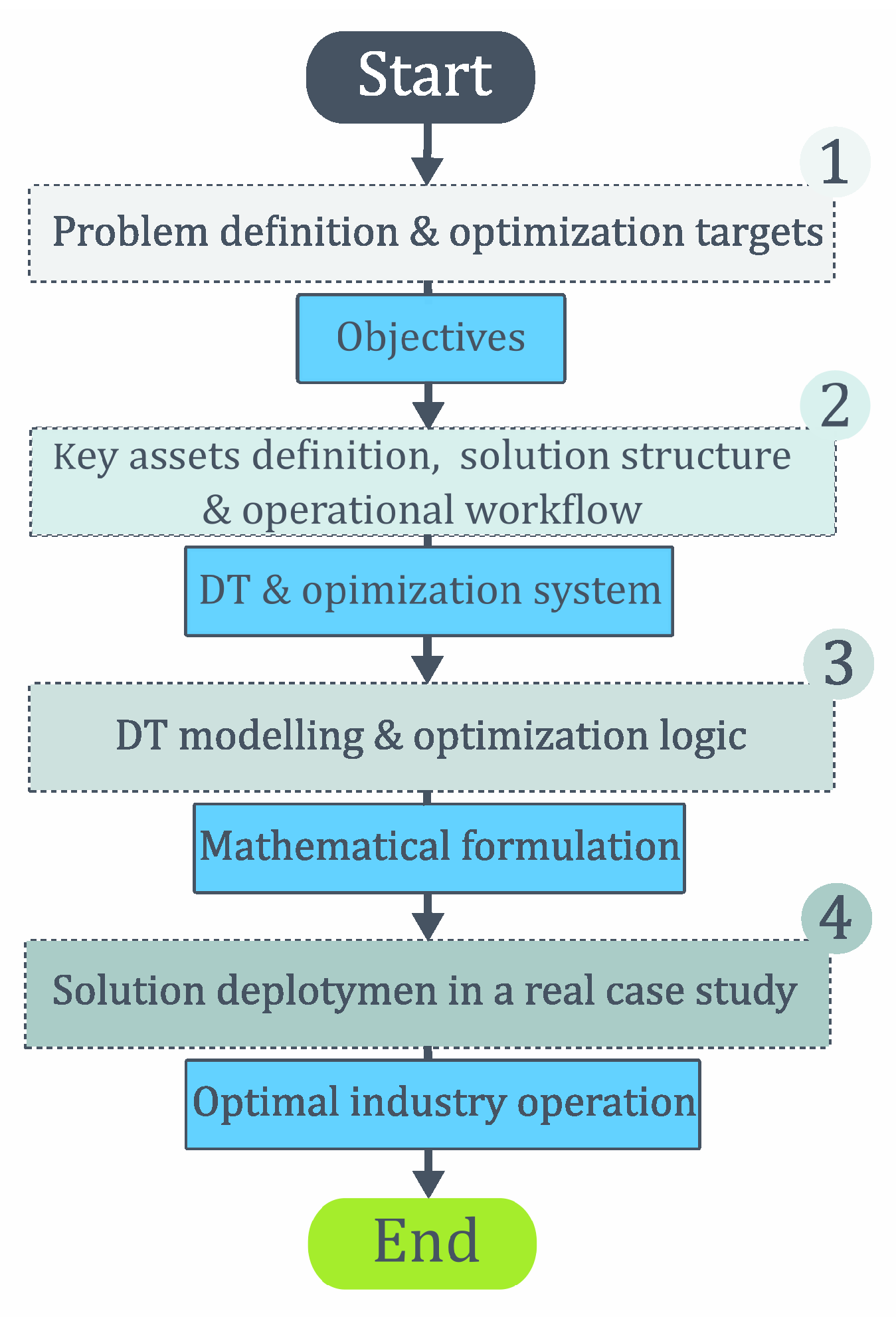
2. Methodology
2.1. Problem Definition and Objectives
- Maximizing the use of on-site renewable energy generation.
- Optimizing EV charging to ensure the highest possible consumption of renewable energy. When this is not feasible, charging is scheduled during periods of low electricity prices and managed to avoid high peak power demands.
- Minimizing EV degradation by analyzing usage patterns, the operation, and charging procedures.
- Efficiently using the SESS to store surplus PV energy and charge from the grid during low-price periods, while also considering system life-cycle impacts.
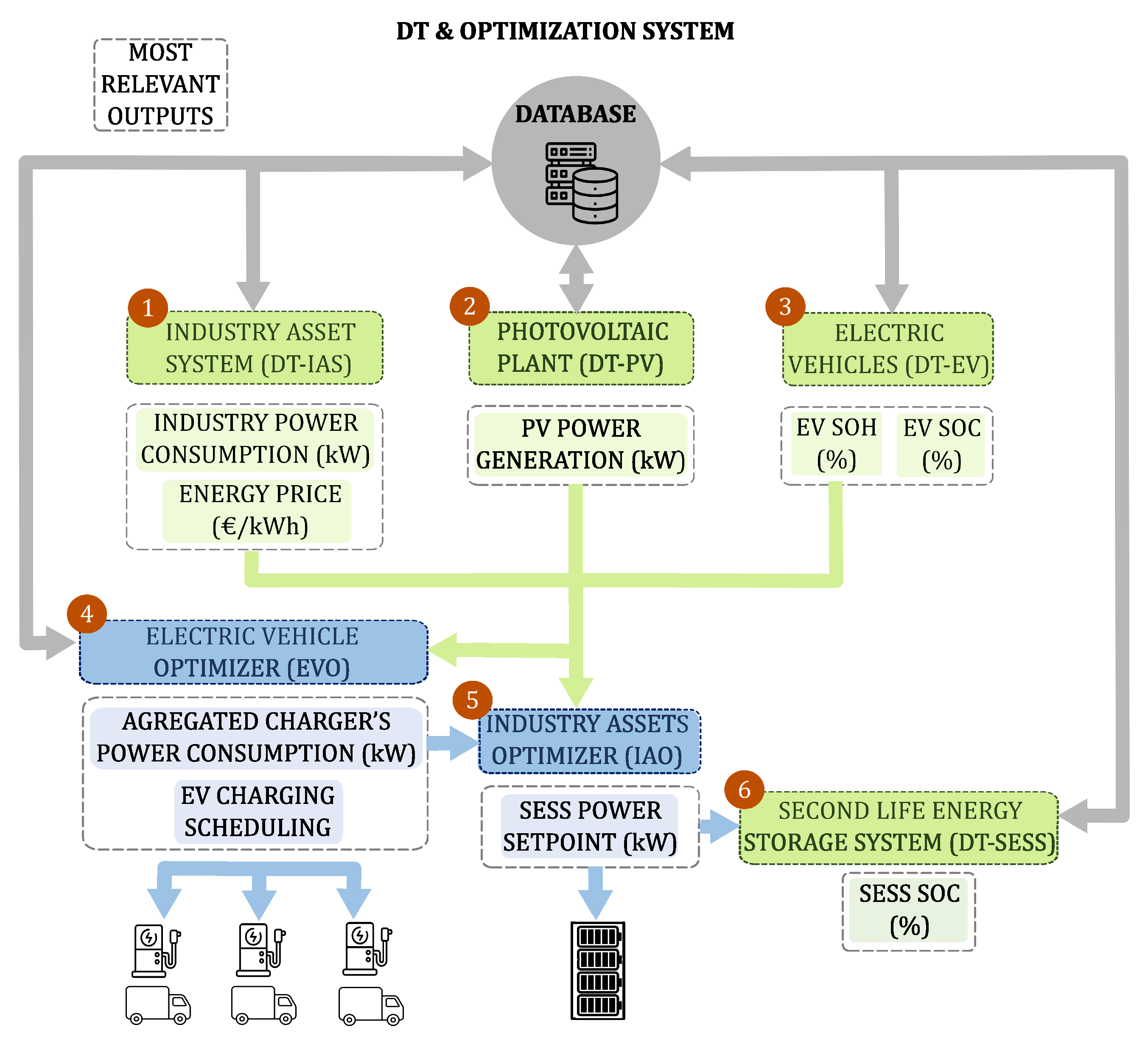
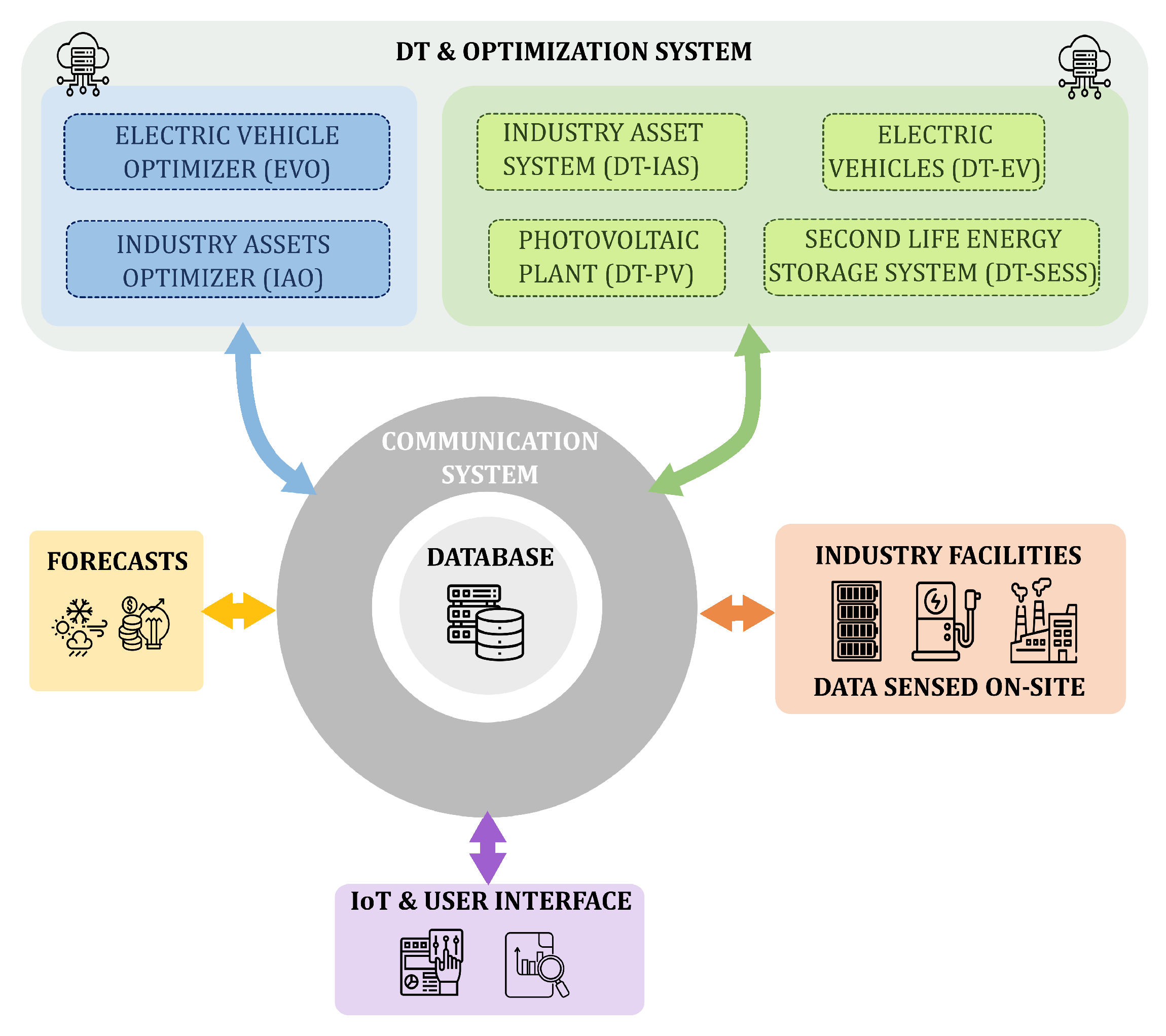
2.2. DT and Optimization System
2.2.1. Digital Twins
- DT-PV: A virtual replica of the photovoltaic system, designed to predict its power generation using weather forecast and other relevant variables.
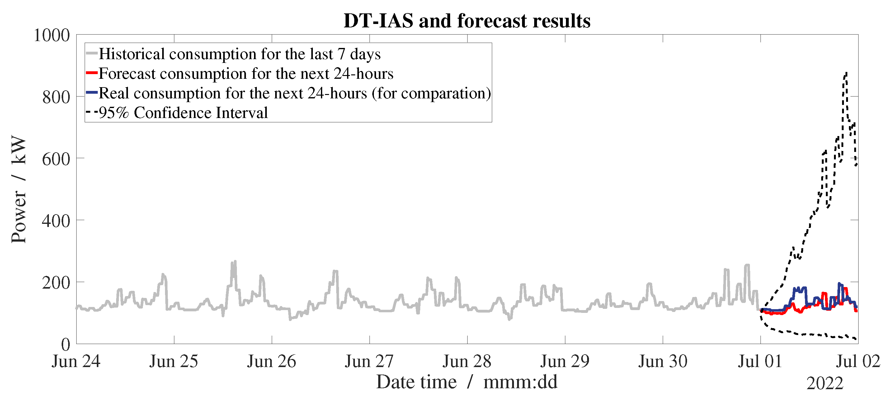
- DT-IAS: Responsible for evaluating and forecasting grid energy prices and power consumption of the Industrial Asset System (IAS), including offices, mechanical workshops, and non-DT-related activities.
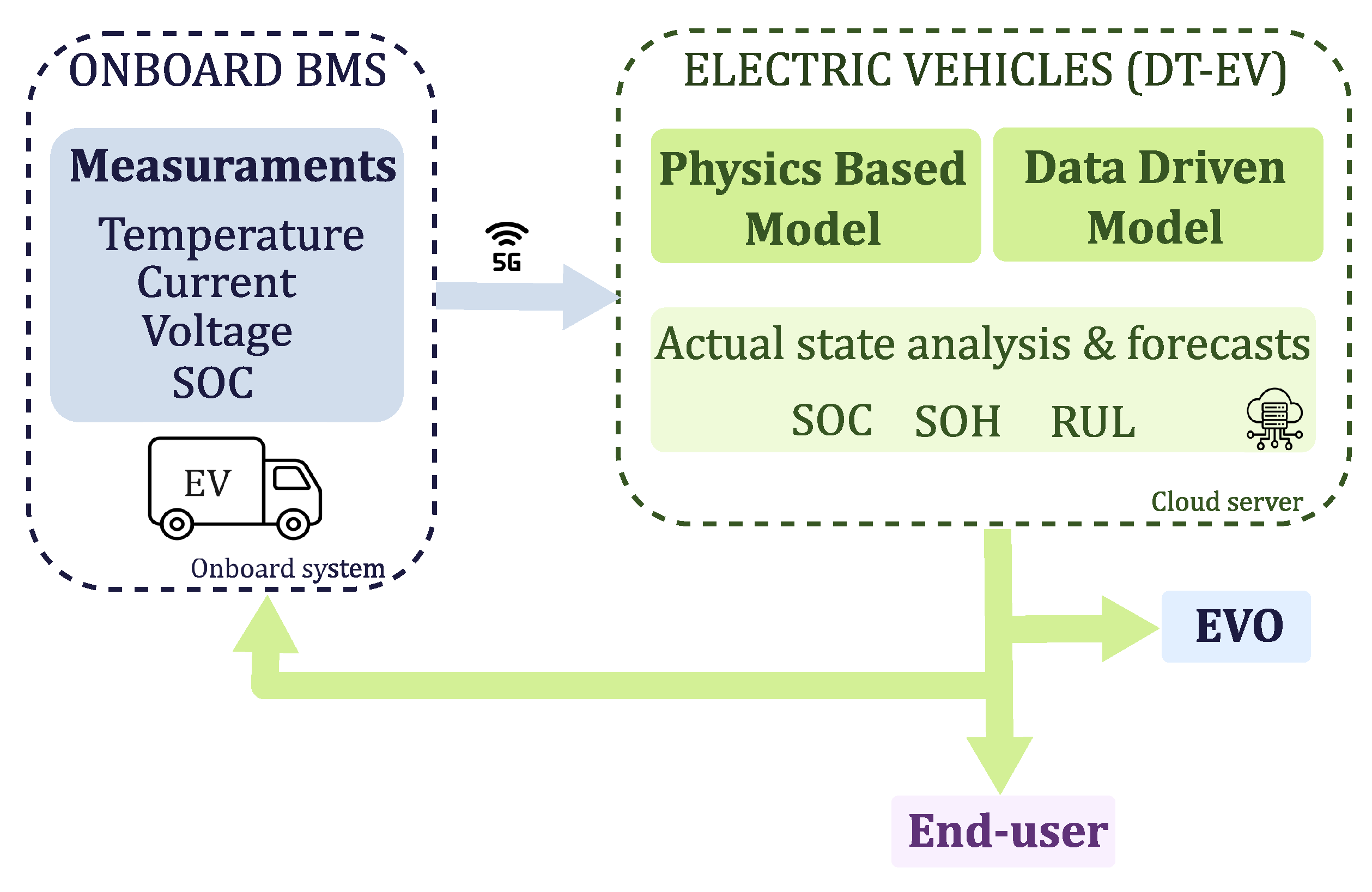
- DT-EV: Each EV within the facility is modeled with a dedicated DT, capable of estimating current SOC and SOH, and predicting future performance under varying usage patterns.
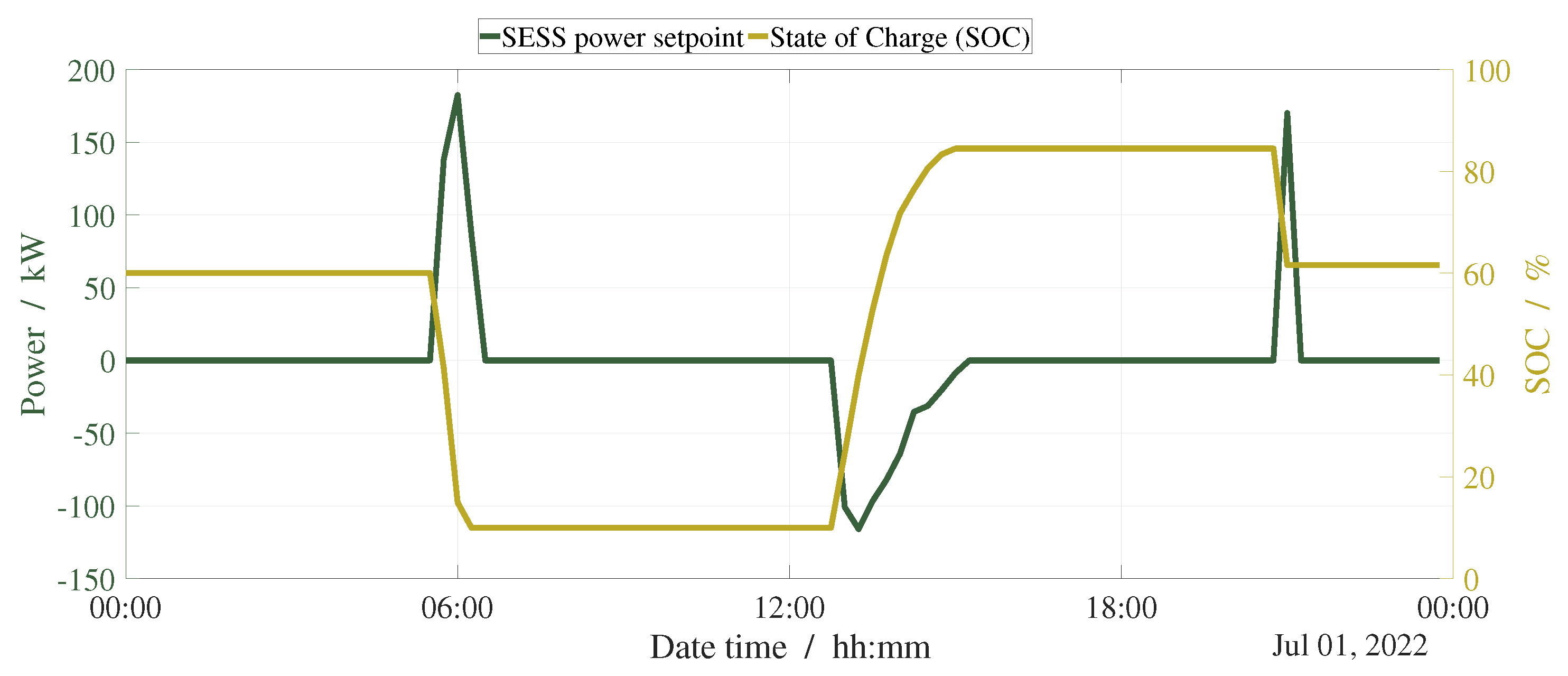
- DT-SESS: This DT monitors the SESS and provides its SOC under operation.
2.2.2. Optimization System
2.2.3. Operational Workflow
3. Mathematical Formulation
3.1. Digital Twins
3.1.1. DT-EV
3.1.2. DT-PV
3.1.3. DT-SESS
3.1.4. DT-IAS
3.2. Optimization System
3.2.1. EVO
- Scheduled trips data (departure and arrival time, distance (km) or energy intensity (kWh)).
- Forecast of the PV energy production, industry demand, and grid energy price, coming from DT-PV, DT-IAS, and day-ahead prices, respectively.
- SOC, SOH, and FEC since EV fleet commissioning, coming from DT-EV.
- SOC of the SESS, coming from DT-SESS.
- A charging profile for each EV.
- Forecast of the aggregated charging power demand for the next 24 h.
3.2.2. IAO
- PV generation forecast.
- Industrial consumption forecast (aggregate consumption of the expected fixed consumption of the industry and the expected EV charging consumption).
- Grid electricity price forecast.
- Emission generation data from the grid, SESS, and PV system.
- SESS battery data, such as initial SOC, operation, and degradation parameters.
- Energy balance: the sum of PV generation, SESS discharge, and grid import must match industrial consumption and EV charging demand.
- SESS operational limits: SOC constraints, charge/discharge power limits, and degradation minimization strategies.
- Grid power constraints: avoiding exceeding contracted power to reduce fixed costs.
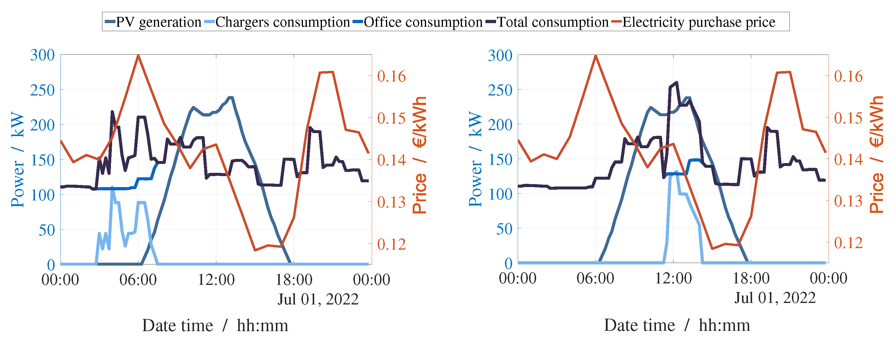
4. Case Study
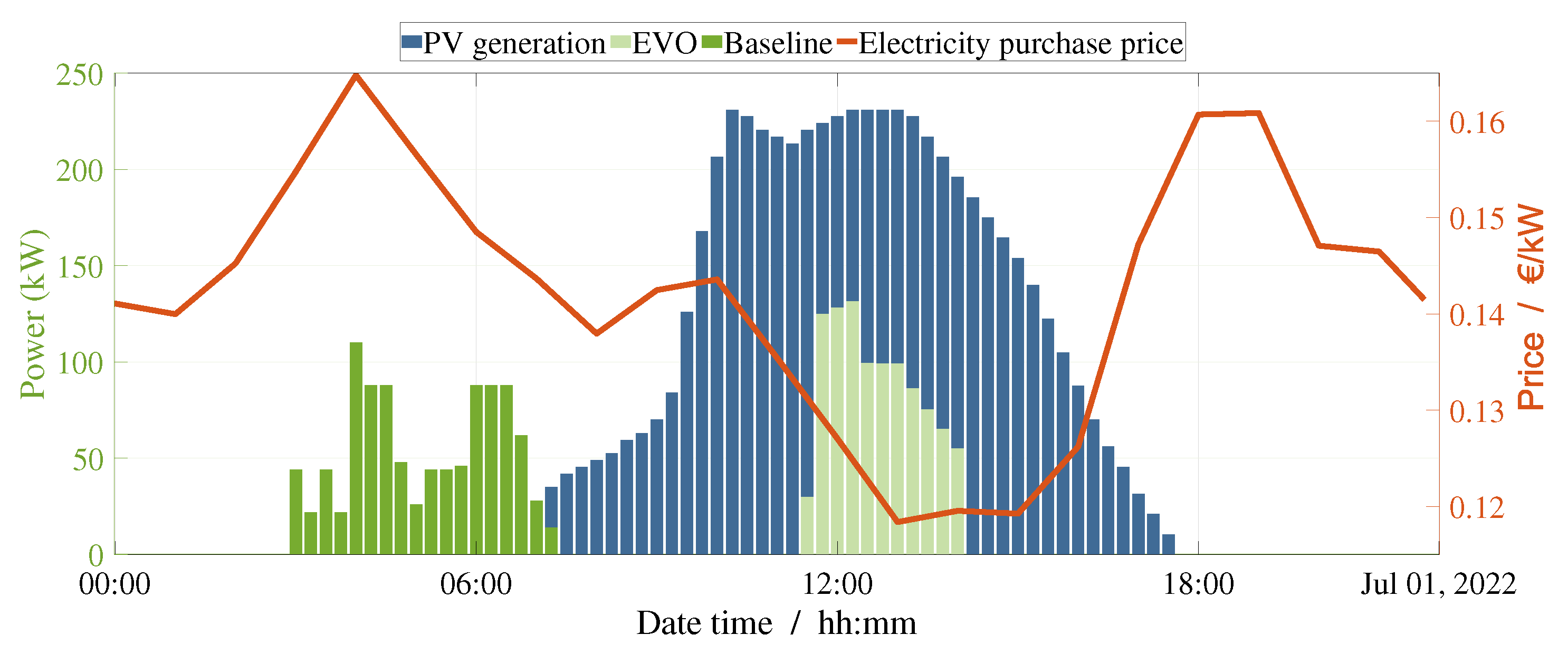
- Baseline: The charging of the EV fleet is not optimized, resulting in nighttime consumption. This reflects actual operational practices of the industry, in which vehicles are connected to charging stations immediately after finishing their routes. Also, SOC is usually kept at high levels.
- EV charging optimization: The EVO is used to optimize the charging of the EV fleet, resulting in charging at the times of higher solar irradiation and lower SOC levels.
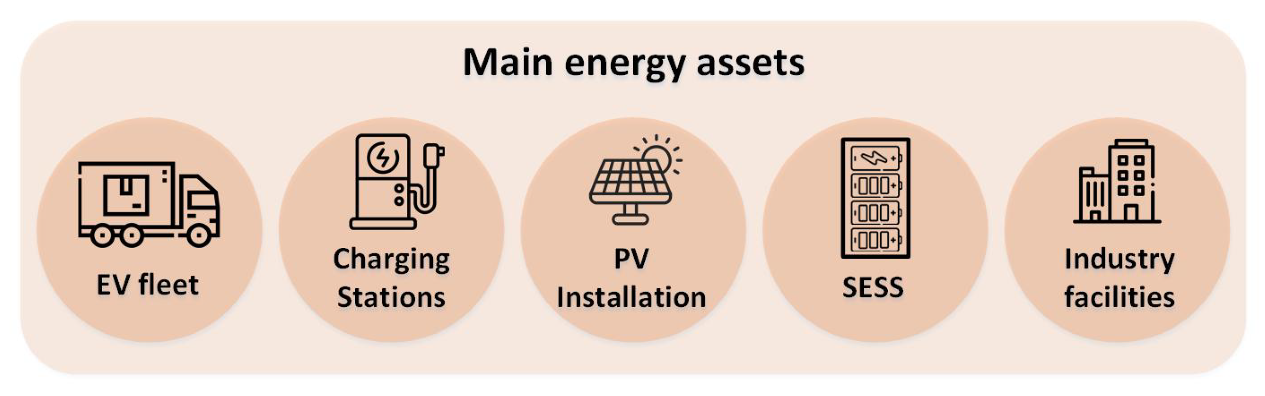
4.1. System Description
4.2. EV Fleet
4.3. Charging Stations
4.4. PV Installation
4.5. SESS
4.6. Industry Facilities
4.7. Communication, Database, Servers, and Ancillary Equipment
- Communication system: Responsible for ensuring the efficient transmission of data between the different systems participating. It collects the information from industrial Supervisory Control and Data Acquisition (SCADA) systems, as well as from sensors associated with PV generation, the SESS, EVs, chargers, and any other relevant facility’s energy consumption. Its primary function is to establish a secure and coherent data flow between physical systems and the cloud while ensuring database integrity. For variables that were not previously digitized, such as electric vehicle monitoring, data loggers have been used.
- Database: It can be considered as the central component of the system, where all the relevant information is stored and acts as an intermediary between cloud-based applications, physical systems, and the user interface. It stores all measured variables from the plant, along with additional relevant data such as weather forecasts and energy prices. Also, the digital twins and optimization algorithms extract the necessary information for the algorithms and store the generated outputs. Subsequently, other applications, including the IoT platform and the user visualization interface, extract from this system the key insights to provide end users useful information about industry status and operation.
- Server and Cloud System: To enable the execution of the different digital twins and optimizers in the cloud, a computational infrastructure is required. In this case, a server, Application Programming Interfaces (API’s), and other tools for orchestrating the different workflows were considered. The server is responsible for hosting and executing the algorithms, while the API functions as a communication interface, facilitating various operations such as triggering DT and optimizers, interacting with the database, and processing data. Since each algorithm deployed in the cloud has distinct execution times, and some rely on the outputs of others, workflow orchestration tools like Apache Airflow (Version 2.5.0) [43] are employed to manage dependencies and ensure efficient task execution.
- IoT platform and user interface: The IoT platform enables the integration of different software tools, leveraging the key outcomes provided by DT and decision support systems. The user interface is responsible for the data visualization and user interaction with the monitored systems, providing access to outputs generated by the cloud-based applications.
5. Results
5.1. Industry Devices Optimization, SESS, PV, and IAS Forecasts
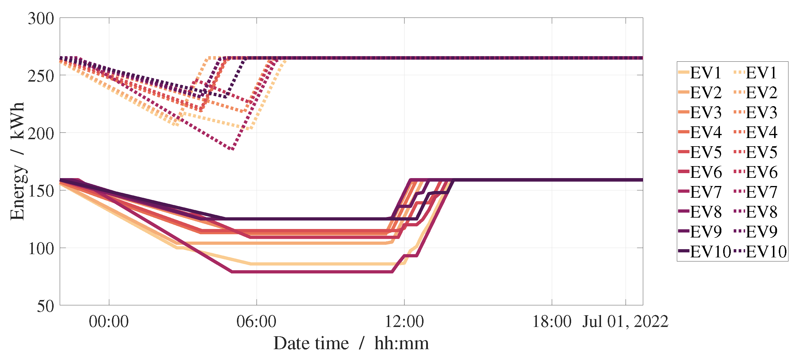
5.2. Electric Vehicle Charging Schedule
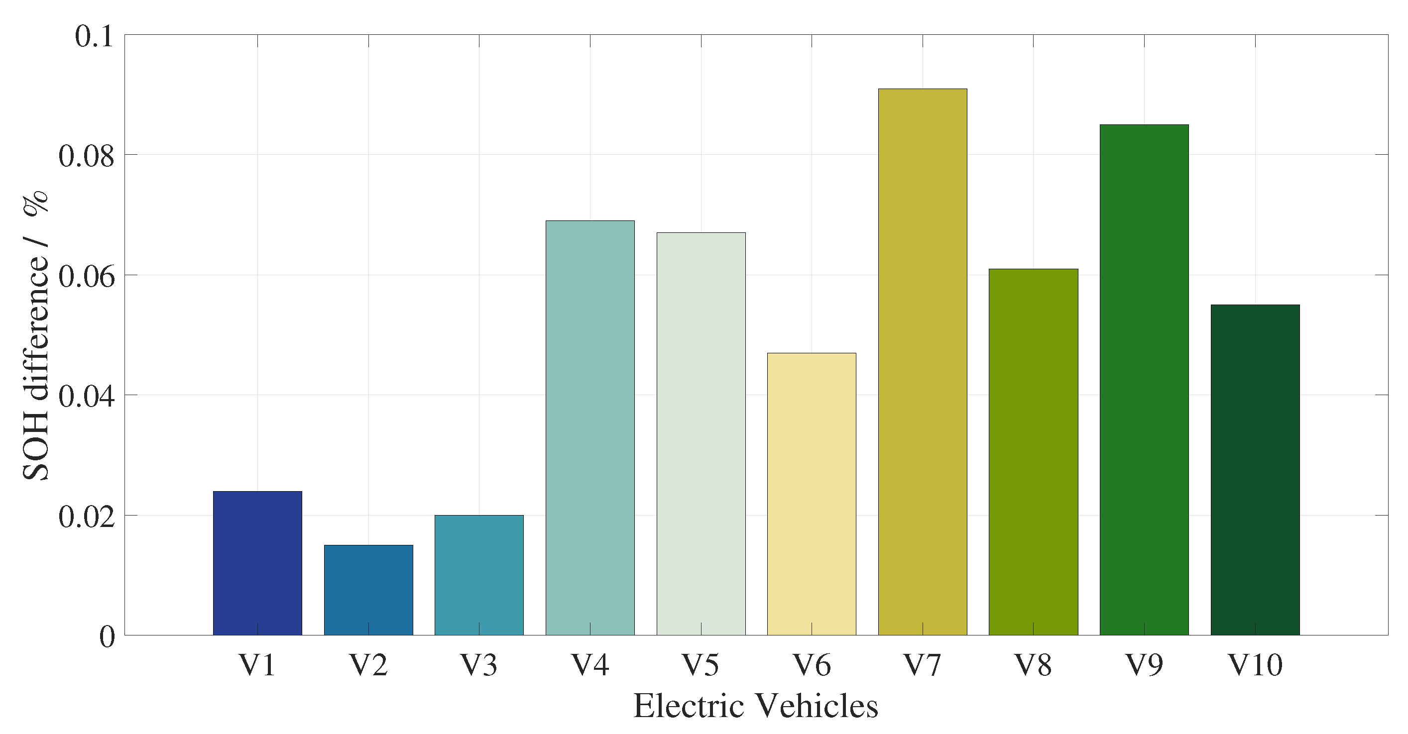
5.3. EV Degradation Analysis and Forecast
6. Conclusions
Author Contributions
Funding
Informed Consent Statement
Data Availability Statement
Acknowledgments
Conflicts of Interest
References
- IEA. Renewables 2024. International Energy Agency, Paris, 2024. Available online: https://www.iea.org/reports/renewables-2024 (accessed on 26 February 2025).
- Thebault, M.; Gaillard, L. Optimization of the integration of photovoltaic systems on buildings for self-consumption–Case study in France. City Environ. Interact. 2021, 10, 100057. [Google Scholar] [CrossRef]
- Tian, J.; Jia, H.; Wang, G.; Huang, Q.; Wu, R.; Gao, H.; Liu, C. Integrated optimization of charging infrastructure, fleet size and vehicle operation in shared autonomous electric vehicle system considering vehicle-to-grid. Renew. Energy 2024, 229, 120760. [Google Scholar] [CrossRef]
- Attaran, M.; Celik, B.G. Digital Twin: Benefits, use cases, challenges, and opportunities. Decis. Anal. J. 2023, 6, 100165. [Google Scholar] [CrossRef]
- Naseri, F.; Gil, S.; Barbu, C.; Cetkin, E.; Yarimca, G.; Jensen, A.; Larsen, P.; Gomes, C. Digital twin of electric vehicle battery systems: Comprehensive review of the use cases, requirements, and platforms. Renew. Sustain. Energy Rev. 2023, 179, 113280. [Google Scholar] [CrossRef]
- Jia, C.; Liu, W.; He, H.; Chau, K. Deep reinforcement learning-based energy management strategy for fuel cell buses integrating future road information and cabin comfort control. Energy Convers. Manag. 2024, 321, 119032. [Google Scholar] [CrossRef]
- Bhatti, G.; Mohan, H.; Raja Singh, R. Towards the future of smart electric vehicles: Digital twin technology. Renew. Sustain. Energy Rev. 2021, 141, 110801. [Google Scholar] [CrossRef]
- Ibrahim, M.; Rjabtšikov, V.; Gilbert, R. Overview of Digital Twin Platforms for EV Applications. Sensors 2023, 23, 1414. [Google Scholar] [CrossRef]
- Francisco, A.M.B.; Monteiro, J.; Cardoso, P.J.S. A Digital Twin of Charging Stations for Fleets of Electric Vehicles. IEEE Access 2023, 11, 125664–125683. [Google Scholar] [CrossRef]
- Iyer, N.G.; Ponnurangan, S.; Abdul Gafoor, N.A.; Rajendran, A.; Lashab, A.; Saha, D.; Guerrero, J.M. A Novel Heuristic Algorithm Integrating Battery Digital-Twin-Based State-of-Charge Estimation for Optimized Electric Vehicle Charging. Electronics 2024, 13, 4412. [Google Scholar] [CrossRef]
- Li, W.; Rentemeister, M.; Badeda, J.; Jöst, D.; Schulte, D.; Sauer, D.U. Digital twin for battery systems: Cloud battery management system with online state-of-charge and state-of-health estimation. J. Energy Storage 2020, 30, 101557. [Google Scholar] [CrossRef]
- Reniers, J.M.; Howey, D.A. Digital twin of a MWh-scale grid battery system for efficiency and degradation analysis. Appl. Energy 2023, 336, 120774. [Google Scholar] [CrossRef]
- Yu, W.; Patros, P.; Young, B.; Klinac, E.; Walmsley, T.G. Energy digital twin technology for industrial energy management: Classification, challenges and future. Renew. Sustain. Energy Rev. 2022, 161, 112407. [Google Scholar] [CrossRef]
- Bécue, A.; Maia, E.; Feeken, L.; Borchers, P.; Praça, I. A New Concept of Digital Twin Supporting Optimization and Resilience of Factories of the Future. Appl. Sci. 2020, 10, 4482. [Google Scholar] [CrossRef]
- Zhang, H.; Liu, Q.; Chen, X.; Zhang, D.; Leng, J. A Digital Twin-Based Approach for Designing and Multi-Objective Optimization of Hollow Glass Production Line. IEEE Access 2017, 5, 26901–26911. [Google Scholar] [CrossRef]
- Florescu, A. Digital Twin for Flexible Manufacturing Systems and Optimization Through Simulation: A Case Study. Machines 2024, 12, 785. [Google Scholar] [CrossRef]
- Lee, D.; Kim, C.K.; Yang, J.; Cho, K.Y.; Choi, J.; Noh, S.D.; Nam, S. Digital Twin-Based Analysis and Optimization for Design and Planning of Production Lines. Machines 2022, 10, 1147. [Google Scholar] [CrossRef]
- Wu, Y.; Guerrero, J.M.; Wu, Y.; Bazmohammadi, N.; Vasquez, J.C.; Cabrera, A.J.; Lu, N. Digital Twins for Microgrids: Opening a New Dimension in the Power System. IEEE Power Energy Mag. 2024, 22, 35–42. [Google Scholar] [CrossRef]
- Özkan, E.; Kök, I.; Özdemır, S. DeepTwin: A Deep Reinforcement Learning Supported Digital Twin Model for Micro-Grids. IEEE Access 2024, 12, 196432–196441. [Google Scholar] [CrossRef]
- Miao, L.; Zhao, J.; Ma, J.; Wei, X.; Hu, Y. Study on Optimization and Scheduling Strategies of Distributed Energy Storage Based on Digital Twin. In Proceedings of the 2024 4th International Conference on Smart Grid and Energy Internet (SGEI), Shenyang, China, 13–15 December 2024; pp. 32–36. [Google Scholar] [CrossRef]
- Yalçin, T.; Paradell Solà, P.; Stefanidou-Voziki, P.; Domínguez-García, J.L.; Demirdelen, T. Exploiting Digitalization of Solar PV Plants Using Machine Learning: Digital Twin Concept for Operation. Energies 2023, 16, 5044. [Google Scholar] [CrossRef]
- Lasseter, R.; Akhil, A.; Marnay, C.; Stephens, J.; Dagle, J.; Guttromsom, R.; Meliopoulos, A.; Yinger, R.; Eto, J. Integration of distributed energy resources. In The CERTS Microgrid Concept; California Energy Commission: Berkeley, CA, USA, 2002. [Google Scholar] [CrossRef]
- Epelle, E.I.; Gerogiorgis, D.I. A computational performance comparison of MILP vs. MINLP formulations for oil production optimisation. Comput. Chem. Eng. 2020, 140, 106903. [Google Scholar] [CrossRef]
- Alemany, J.; Kasprzyk, L.; Magnago, F. Effects of binary variables in mixed integer linear programming based unit commitment in large-scale electricity markets. Electr. Power Syst. Res. 2018, 160, 429–438. [Google Scholar] [CrossRef]
- Ham, A.; Park, M.J.; Kim, K. Energy-Aware Flexible Job Shop Scheduling Using Mixed Integer Programming and Constraint Programming. Math. Probl. Eng. 2021, 2021, 1–12. [Google Scholar] [CrossRef]
- Bernabeu, A.; Clemente, A.; Díaz, F.; Trilla, L. Experimental data granularity studies for the development of NMC Li-ion battery models. In Proceedings of the IECON 2024-50th Annual Conference of the IEEE Industrial Electronics Society, Chicago, IL, USA, 3–6 November 2024; pp. 1–7. [Google Scholar] [CrossRef]
- Montes, T.; Etxandi-Santolaya, M.; Eichman, J.; Ferreira, V.J.; Trilla, L.; Corchero, C. Procedure for Assessing the Suitability of Battery Second Life Applications after EV First Life. Batteries 2022, 8, 122. [Google Scholar] [CrossRef]
- Ji, C.; Dai, J.; Zhai, C.; Wang, J.; Tian, Y.; Sun, W. A Review on Lithium-Ion Battery Modeling from Mechanism-Based and Data-Driven Perspectives. Processes 2024, 12, 1871. [Google Scholar] [CrossRef]
- Chaturvedi, N.A.; Klein, R.; Christensen, J.; Ahmed, J.; Kojic, A. Algorithms for Advanced Battery-Management Systems. IEEE Control Syst. Mag. 2010, 30, 49–68. [Google Scholar] [CrossRef]
- Heinrich, F.; Klapper, P.; Pruckner, M. A comprehensive study on battery electric modeling approaches based on machine learning. Energy Inform. 2021, 4, 17. [Google Scholar] [CrossRef]
- Chen, C.H.; Brosa Planella, F.; O’Regan, K.; Gastol, D.; Widanage, W.D.; Kendrick, E. Development of Experimental Techniques for Parameterization of Multi-scale Lithium-ion Battery Models. J. Electrochem. Soc. 2020, 167, 080534. [Google Scholar] [CrossRef]
- Timms, R.; Marquis, S.G.; Sulzer, V.; Please, C.P.; Chapman, S.J. Asymptotic Reduction of a Lithium-Ion Pouch Cell Model. SIAM J. Appl. Math. 2021, 81, 765–788. [Google Scholar] [CrossRef]
- Marquis, S.G. Long-Term Degradation of Lithium-Ion Batteries. Ph.D. Thesis, University of Oxford, Oxford, UK, 2020. [Google Scholar]
- O’Kane, S.E.J.; Ai, W.; Madabattula, G.; Alonso-Alvarez, D.; Timms, R.; Sulzer, V.; Edge, J.S.; Wu, B.; Offer, G.J.; Marinescu, M. Lithium-ion battery degradation: How to model it. Phys. Chem. Chem. Phys. 2022, 24, 7909–7922. [Google Scholar] [CrossRef]
- Jafari, S.; Byun, Y.C. Optimizing Battery RUL Prediction of Lithium-Ion Batteries Based on Harris Hawk Optimization Approach Using Random Forest and LightGBM. IEEE Access 2023, 11, 87034–87046. [Google Scholar] [CrossRef]
- Sulzer, V.; Marquis, S.G.; Timms, R.; Robinson, M.; Chapman, S.J. Python Battery Mathematical Modelling (PyBaMM). J. Electrochem. Soc. 2021, 9, 14. [Google Scholar] [CrossRef]
- Pedregosa, F.; Varoquaux, G.; Gramfort, A.; Michel, V.; Thirion, B.; Grisel, O.; Blondel, M.; Prettenhofer, P.; Weiss, R.; Dubourg, V.; et al. Scikit-learn: Machine Learning in Python. J. Mach. Learn. Res. 2011, 12, 2825–2830. [Google Scholar]
- Borrego-Orpinell, G.; Forero, J.F.; Caprara, A.; Díaz-González, F. Impact Assessment of Second-Life Batteries and Local Photovoltaics for Decarbonizing Enterprises Through System Digitalization and Energy Management. Energies 2025, 18, 1198. [Google Scholar] [CrossRef]
- Sen, P.; Roy, M.; Pal, P. Application of ARIMA for forecasting energy consumption and GHG emission: A case study of an Indian pig iron manufacturing organization. Energy 2016, 116, 1031–1038. [Google Scholar] [CrossRef]
- Stroe, D.I.; Swierczynski, M.; Stroe, A.I.; Teodorescu, R.; Laerke, R.; Kjaer, P.C. Degradation behaviour of Lithium-ion batteries based on field measured frequency regulation mission profile. In Proceedings of the 2015 IEEE Energy Conversion Congress and Exposition (ECCE), Montreal, QC, Canada, 20–24 September 2015; pp. 14–21. [Google Scholar] [CrossRef]
- Montes, T.; Pinsach Batet, F.; Igualada, L.; Eichman, J. Degradation-conscious charge management: Comparison of different techniques to include battery degradation in Electric Vehicle Charging Optimization. J. Energy Storage 2024, 88, 111560. [Google Scholar] [CrossRef]
- Trucks, R. D26 ZE LEC Spec Sheet 2022, 2022. Available online: https://www.renault-trucks.co.uk/sites/default/files/2022-05/D26%20ZE%20LEC%20Spec%20Sheet%202022.pdf (accessed on 23 March 2025).
- Apache Airflow, Version 2.5.0. Apache Software Foundation, 2015. Available online: https://airflow.apache.org (accessed on 15 January 2025).
- Li, Y.; Guo, W.; Stroe, D.I.; Zhao, H.; Kjær Kristensen, P.; Rosgaard Jensen, L.; Pedersen, K.; Gurevich, L. Evolution of aging mechanisms and performance degradation of lithium-ion battery from moderate to severe capacity loss scenarios. Chem. Eng. J. 2024, 498, 155588. [Google Scholar] [CrossRef]
- Wei, Y.; Yao, Y.; Pang, K.; Xu, C.; Han, X.; Lu, L.; Li, Y.; Qin, Y.; Zheng, Y.; Wang, H.; et al. A Comprehensive Study of Degradation Characteristics and Mechanisms of Commercial Li(NiMnCo)O2 EV Batteries under Vehicle-To-Grid (V2G) Services. Batteries 2022, 8, 188. [Google Scholar] [CrossRef]


| Industry consumption | |
| Electric trucks, gas-powered trucks, | ∼300 kW averaged |
| and office assets power () | |
| Annual energy consumption () | 2570 MWh |
| Contracted grid power () | 380 kW |
| PV generation | |
| Peak PV power capacity () | 333 kWp |
| Individual inverter nominal power () | 100 kW |
| Number of PV inverters in parallel () | 3 units |
| Annual PV energy generated () | 310 MWh |
| Second-life energy storage system | |
| Capacity () | 166 kWh |
| Power () | 191 kW |
| Cells in series () | 76 |
| Cells in parallel () | 8 |
| Maximum battery voltage () | 304 V |
| Minimum battery voltage () | 212.8 V |
| Rated battery voltage () | 250.2 V |
| Maximum battery current () | 720 A |
| Battery price per kWh () | 90 EUR/kWh |
| Battery price () | 14,955 EUR |
| Remaining battery cycles () | 1000 cycles |
| Electric vehicles and chargers | |
| Vehicle model | D WIDE ZE |
| EV battery capacity () [42] | 265 kWh |
| Number of modules per EV [42] | 4 |
| EV unitary module capacity [42] | 66 kWh |
| EV cell specifications [42] | NMC |
| Number of EV considered (m) | 10 |
| Number of chargers available (c) | 10 |
| Maximum charging power () | 22 kW |
| Trip | Departure | Arrival | Vehicle |
|---|---|---|---|
| 1 | 22:00 | 03:00 | V7 |
| 2 | 22:00 | 03:00 | V2 |
| 3 | 22:00 | 04:00 | V1 |
| 4 | 22:15 | 04:00 | V4 |
| 5 | 22:15 | 04:30 | V10 |
| 6 | 22:15 | 04:00 | V5 |
| 7 | 22:15 | 05:00 | V6 |
| 8 | 22:30 | 03:30 | V3 |
| 9 | 22:45 | 04:00 | V9 |
| 10 | 23:00 | 05:15 | V8 |
| 11 | 03:15 | 06:00 | V2 |
| 12 | 03:45 | 06:00 | V3 |
| 13 | 04:30 | 05:45 | V1 |
| Case | Baseline | EVO | Save |
|---|---|---|---|
| 1 day | EUR 132.4 | EUR 108.2 | 18.3% |
| 3 days | EUR 1016.7 | EUR 1228.7 | 17.3% |
| 5 days | EUR 2896.1 | EUR 3435.5 | 15.7% |
| Number of EVs | 10 | 20 | 30 | 40 | 50 | 60 | 70 | 80 | 90 | 100 |
| Exec. time (s) | 1.5 | 2.4 | 3.8 | 5.8 | 9.0 | 13.8 | 21.4 | 33 | 50 | 80 |
Disclaimer/Publisher’s Note: The statements, opinions and data contained in all publications are solely those of the individual author(s) and contributor(s) and not of MDPI and/or the editor(s). MDPI and/or the editor(s) disclaim responsibility for any injury to people or property resulting from any ideas, methods, instructions or products referred to in the content. |
© 2025 by the authors. Licensee MDPI, Basel, Switzerland. This article is an open access article distributed under the terms and conditions of the Creative Commons Attribution (CC BY) license (https://creativecommons.org/licenses/by/4.0/).
Share and Cite
Bernabeu-Santisteban, A.; Henao-Muñoz, A.C.; Borrego-Orpinell, G.; Díaz-González, F.; Heredero-Peris, D.; Trilla, L. Energy Management System for Renewable Energy and Electric Vehicle-Based Industries Using Digital Twins: A Waste Management Industry Case Study. Appl. Sci. 2025, 15, 7351. https://doi.org/10.3390/app15137351
Bernabeu-Santisteban A, Henao-Muñoz AC, Borrego-Orpinell G, Díaz-González F, Heredero-Peris D, Trilla L. Energy Management System for Renewable Energy and Electric Vehicle-Based Industries Using Digital Twins: A Waste Management Industry Case Study. Applied Sciences. 2025; 15(13):7351. https://doi.org/10.3390/app15137351
Chicago/Turabian StyleBernabeu-Santisteban, Andrés, Andres C. Henao-Muñoz, Gerard Borrego-Orpinell, Francisco Díaz-González, Daniel Heredero-Peris, and Lluís Trilla. 2025. "Energy Management System for Renewable Energy and Electric Vehicle-Based Industries Using Digital Twins: A Waste Management Industry Case Study" Applied Sciences 15, no. 13: 7351. https://doi.org/10.3390/app15137351
APA StyleBernabeu-Santisteban, A., Henao-Muñoz, A. C., Borrego-Orpinell, G., Díaz-González, F., Heredero-Peris, D., & Trilla, L. (2025). Energy Management System for Renewable Energy and Electric Vehicle-Based Industries Using Digital Twins: A Waste Management Industry Case Study. Applied Sciences, 15(13), 7351. https://doi.org/10.3390/app15137351