Design of a Bionic Self-Insulating Mechanical Arm for Concealed Space Inspection in the Live Power Cable Tunnels

Abstract

Adopting mobile robots for high voltage (HV) live-line operations can mitigate personnel casualties and enhance operational efficiency. However, conventional mechanical arms cannot inspect concealed spaces in the power cable tunnel because their joint integrates metallic motors or hydraulic serial-drive mechanisms, which limit the arm’s length and insulation performance. Therefore, this study proposes a 7-degree-of-freedom (7-DOF) bionic mechanical arm with rigid-flexible coupling, mimicking human arm joints (shoulder, elbow, and wrist) designed for HV live-line operations in concealed cable tunnels. The arm employs a tendon-driven mechanism to remotely actuate joints, analogous to human musculoskeletal dynamics, thereby physically isolating conductive components (e.g., motors) from the mechanical arm. The arm’s structure utilizes dielectric materials and insulation-optimized geometries to reduce peak electric field intensity and increase creepage distance, achieving intrinsic self-insulation. Furthermore, the mechanical design addresses challenges posed by concealed spaces (e.g., shield tunnels and multi-circuit cable layouts) through the analysis of joint kinematics, drive mechanisms, and dielectric performance. The workspace of the proposed arm is an oblate ellipsoid with minor and major axes measuring 1.25 m and 1.65 m, respectively, covering the concealed space in the cable tunnel, while the arm’s quality is 4.7 kg. The maximum electric field intensity is 74.3 kV/m under 220 kV operating voltage. The field value is less than the air breakdown threshold. The proposed mechanical arm design significantly improves spatial adaptability, operational efficiency, and reliability in HV live-line inspection, offering theoretical and practical advancements for intelligent maintenance in cable tunnel environments.

1. Introduction

With rapid socio-economic development and industrialization, power cables have become a critical component of modern transmission systems [1,2,3,4]. Power cable tunnels often feature complex architectures, such as shield tunnels, jacked pipes, and multi-tiered racks, resulting in intertwined cable layouts that form concealed spaces [5,6]. Conventional inspection methods rely on fixed-route patrols and handheld sensors positioned close to the sensor carriers instead of the cables [7,8]. Consequently, these approaches fail to detect defects in concealed areas, including insulation layer breaches, metal sheath corrosion, or carbonization of cable jackets caused by discharge on support structures. Such limitations significantly compromise the quality and safety management of high-voltage (HV) cable maintenance [9]. Therefore, we propose a methodology that enables sensors to operate close to cable surfaces to achieve comprehensive, blind-zone-free monitoring.

The methodology aims at close-range, full-coverage inspection of high-voltage cable jackets under live-line operating conditions. Replacing manual labor with robotic systems can mitigate personnel risks, enhance operational safety, and improve efficiency, offering economic and practical advantages [10,11]. Consequently, the live-line inspection robot with a multi-freedom degrees mechanic arm is selected as the carrier for the cable surface. Japan’s Phase II robot [12], Shandong University’s live-line repair robot [13], and Korea’s insulator-cleaning robot [14] are the typical models among all the robots used for power system live maintenance [15,16,17,18]. However, these robots employ metallic mechanical arms with base-mounted insulation layers. The extra insulation layer gives the mechanical arm excessive mass and volume [19]. Therefore, the arm’s length is limited and cannot accurately inspect boundary features in concealed spaces (e.g., cable bends or pipe intersections) or detect visual blind spots (e.g., jacket wear on tunnel-facing surfaces) [20,21]. In addition, the conventional metallic arm directly connected to the HV electrode leads to the following challenges. First, the corona discharge is likely to occur at any location with slight curvature according to the position and orientation of the arm [22]. Therefore, the corona mitigation measurement (e.g., corona ring) cannot be effectively installed at a fixed location of the arm [23,24]. Second, due to its dimension limitation, the insulation layer cannot provide sufficient leakage distance for arc creepage [25,26,27]. Third, the motor and the controller malfunctions are likely to occur since the motor performance at the joint is affected by the electric field along the arm [28,29,30,31].

To address all the challenges mentioned above, this study develops a bionic mechanical arm with self-insulating capabilities, mimicking the kinematic structure of human arms with the shoulder, elbow, and wrist joints. The joint is made of rigid insulating material (e.g., porcelain and epoxy) and driven by the insulating flexible material (e.g., polyester rope). Therefore, the mass of the proposed arm is significantly less than the conventional metallic arm. The material’s low mass enables the arm to extend further, providing a longer creepage distance and greater working space than conventional metal arms.

Compared with conventional live-working manipulators, the self-insulated cable-driven manipulator designed in this manuscript exhibits multiple differences, mainly in terms of insulation performance, application scenarios, structure, and mass.

First, regarding self-insulation performance: Although conventional live-working manipulators have insulation designs, their motor actuators, manipulator skeletons, and other conductive components are still distributed on the manipulator body. Therefore, the manipulator lacks self-insulation performance. In this case, extra insulation designs for the manipulator on the mechanical arm need to be added to enhance insulation performance, and most arms of this type are limited to a voltage level of 10 kV. However, the self-insulated manipulator uses epoxy resin as the rigid material and polyester fiber as the flexible material for the manipulator body. Consequently, this manipulator not only requires no additional insulation design but can also adapt to working environments with a high voltage level of 220 kV.

Second, in terms of manipulator mass: Conventional manipulators typically need to mount drive motors at the joints, which increases the mass of the mechanical arm. The self-insulated manipulator has significantly reduced its own mass because the design separates the drive motors from the body. This results in minimal changes in the center of gravity during the movement of the entire arm, and its small inertia tensor imposes low performance requirements on the lower mobile platform. This also means that during the operation of the entire machine, the multi-rigid-body kinematic analysis of the manipulator body can be almost omitted.

Finally, although the self-insulated mechanical arm cannot complete the tasks such as cable cutting and splicing due to its relatively small load capacity, its insulation performance makes it more suitable for sensing, monitoring, and fault detection in high-voltage environments. The specific comparisons between the conventional live-working manipulator and the self-insulated cable-driven manipulator are shown in

Table 1. Comparison of typical global-mapping-based range perception methods.

Mechanical Arm Type	Cables Repairing Robot	Live Line Robot	Self-Insulating Type
Features
Structure
Self-insulating	×	×	√
Capable of live operation	√	√	√
Adapt to the maximum voltage level	10 kV	10 kV	220 kV
Capable of high voltage sensing detection	√	√	√
Capable of cable cutting and other operations	√	√	×
The drive motor is separated from the robot body	×	×	√
Mass of a single robotic arm	---	45.2 kg	4.7 kg
DOF	3	6	7
Work space (m3)	1.2	0.85	1.4

.

2. Methods

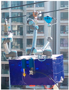
In response to the inspection needs in the cable tunnel shown in Figure 1, we have made a series of designs for this self-insulating mechanical arm. The design of the bionic insulation arm incorporates a tendon-driven mechanism to simulate musculoskeletal actuation, physically isolating conductive components (e.g., motors) from the arm’s dielectric body. Both materials and structural design prioritize electrical insulation, ensuring full-body dielectric performance.

The Mechanical arm employs a comprehensive 7-degree-of-freedom (7-DOF) linkage model to replicate the complex kinematics of human arm movements, comprising the following:

• Three DOFs at the wrist joint (enabling pitch, yaw, and roll);
• One simplified DOF at the elbow joint (flexion/extension only);
• Three DOFs at the shoulder joint (omnidirectional orientation).

Design emphasis is placed on the 3 DOF mechanisms of the wrist and shoulder joints to maximize dexterity in confined spaces.

To achieve the design target of self-insulation, the mechanical arm eliminates joint-mounted motors—a critical limitation in conventional designs. Drawing inspiration from musculoskeletal systems, we implement a tendon-driven parallel mechanism that replicates the full range of motion in both shoulder and wrist joints while maintaining complete electrical isolation. This biomimetic approach simultaneously decouples conductive components (e.g., motors) from the dielectric structure, preserves anthropomorphic flexibility through cable-pulley force transmission, and reduces inertial loads via distributed actuation. The resulting architecture combines the dexterity of human-like movement with the essential dielectric properties required for live-line operation.

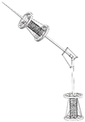
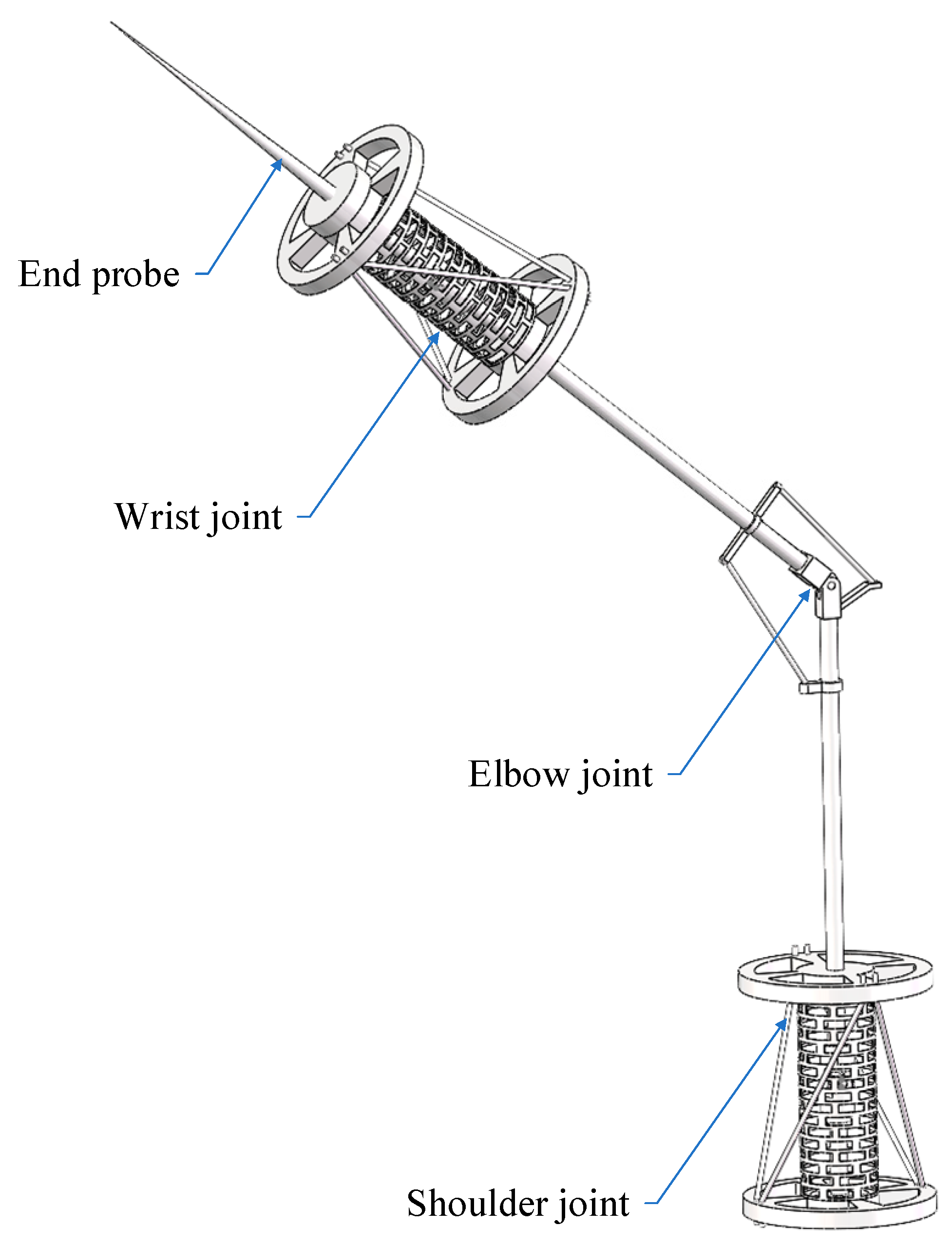
Since the mechanical arm requires self-insulating properties, conventional drive motors cannot be directly mounted on the joints. Therefore, this manuscript adopts a cable-driven mechanism to simulate the omnidirectional movement of the shoulder and wrist joints to achieve performance and flexibility similar to a muscle-driven system. As shown in Figure 2, the self-insulating mechanical arm consists of a 3-DOF biomimetic self-insulating joint serving as the shoulder and elbow, connected by a 1-DOF elbow joint.

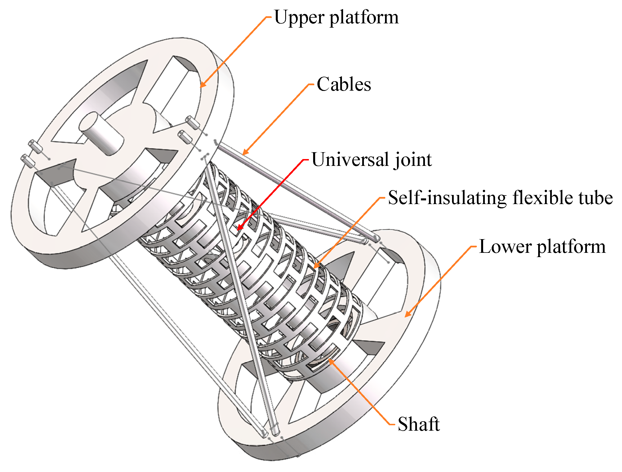
To mimic the three-degree-of-freedom (3-DOF) roll, pitch, and yaw movements of the human arm’s shoulder and wrist joints, a biomimetic self-insulating joint mechanism was designed, as illustrated in Figure 3.

The joint mechanism consists of a fixed platform and a moving platform. A concentric, self-insulating, flexible body is arranged to provide mechanical support. Two concentric shafts inside the flexible body further reinforce the structure, connected via a universal joint. The upper shaft, made of insulating material, passes through the upper platform. Thus, the moving platform is cable-driven and connected to the fixed platform via the self-insulating flexible body, providing support. A rotary bearing is also embedded between the universal joint support rod and the moving platform, enabling relative rotational motion between the moving platform and either the flexible body or the fixed platform. The rotating shaft restricts the lateral bending of the flexible body, effectively simplifying inverse kinematics modeling and computation.

The upper and lower platforms are affixed with insulating plates to enhance electrical insulation. A combined bearing links the upper moving platform to the insulating plate, facilitating rotational and translational motions. The mechanism is driven by four cables, allowing the moving platform to achieve 3-DOF roll, pitch, and yaw movements under tension.

3. Kinematics Modeling of Self-Insulating Mechanical Arm Joints

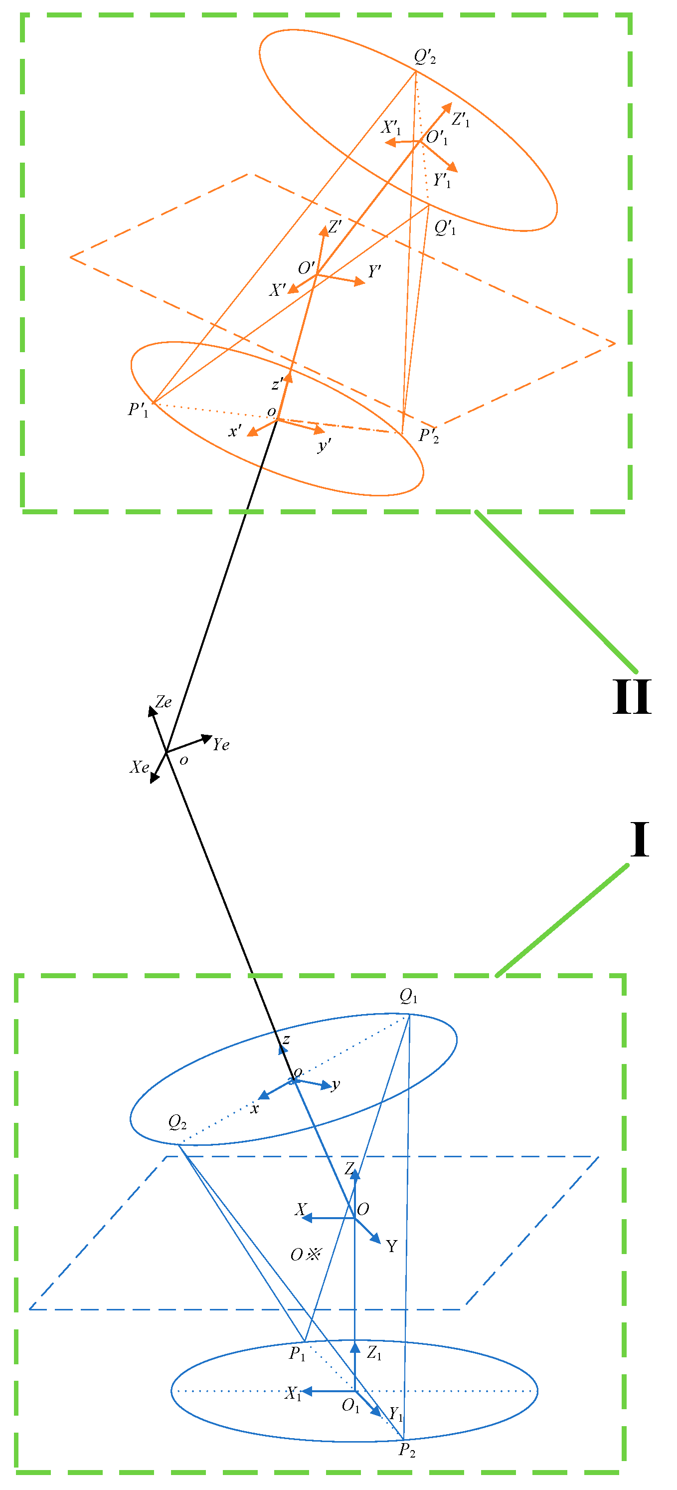
According to the self-insulating mechanical joint design described above, a simplified structure diagram of the entire robotic arm was established, as shown in Figure 4. Since wrist joint part I is exactly the same as shoulder joint part II, and the elbow joint has only one degree of freedom, the shoulder joint is modeled and analyzed separately, as shown in Figure 5.

The simplified model considers the cables, platforms, and connecting rods while neglecting their masses and diameters. The four cables in the kinematic model are assumed to be massless with negligible diameter, having their lower platform attachment points defined as P₁ and P₂ and upper platform points as Q₁ and Q₂. Both the fixed and moving platforms are treated as reference points with negligible thickness.

The fixed platform’s local coordinate system O₁X₁Y₁Z₁ has its origin O₁ at the platform center, with the Y₁-axis oriented along the O₁P₂ direction and the X₁-axis perpendicular to Y₁. The Z₁-axis follows the right-hand rule. Similarly, the moving platform’s local coordinate system oxyz is defined.

Dielectric plates are attached to both platforms’ surfaces to provide electrical insulation during live-line operations. In the initial configuration, the connection lines between attachment points on the moving and fixed platforms remain perpendicular. The distances from points P and Q to their respective platform centers are denoted as p and q, while L represents the cable length between corresponding P and Q points. Each cable’s tension force is represented by T, and its directional unit vector is defined as uᵢ.

The model maintains the following essential characteristics: cable-driven actuation through the four tension elements, orthogonal initial alignment of the platform connection lines, and incorporated dielectric insulation through the attached plates. The coordinate system definitions and geometric parameters establish the foundation for subsequent kinematic analysis while preserving the self-insulating properties of the joint mechanism.

3.1. Forward Kinematics

The homogeneous coordinates of P₁ and P₂ in the fixed platform’s global coordinate system OXYZ are denoted as ^Op₁ and ^Op₂, while Q₁ and Q₂’s coordinates in the moving platform’s local frame oxyz are expressed as ^oq₁ and ^oq₂, respectively:

$$\begin{array}{l}{}^O\mathit{p}_1={(0,-p,-d_1,1)}^T,{}^O\mathit{p}_2={(0,p,-d_1,1)}^T\\ {}^o\mathit{q}_1={(-q,0,0,1)}^T,{}^o\mathit{q}_2={(q,0,0,1)}^T\end{array}$$

(1)

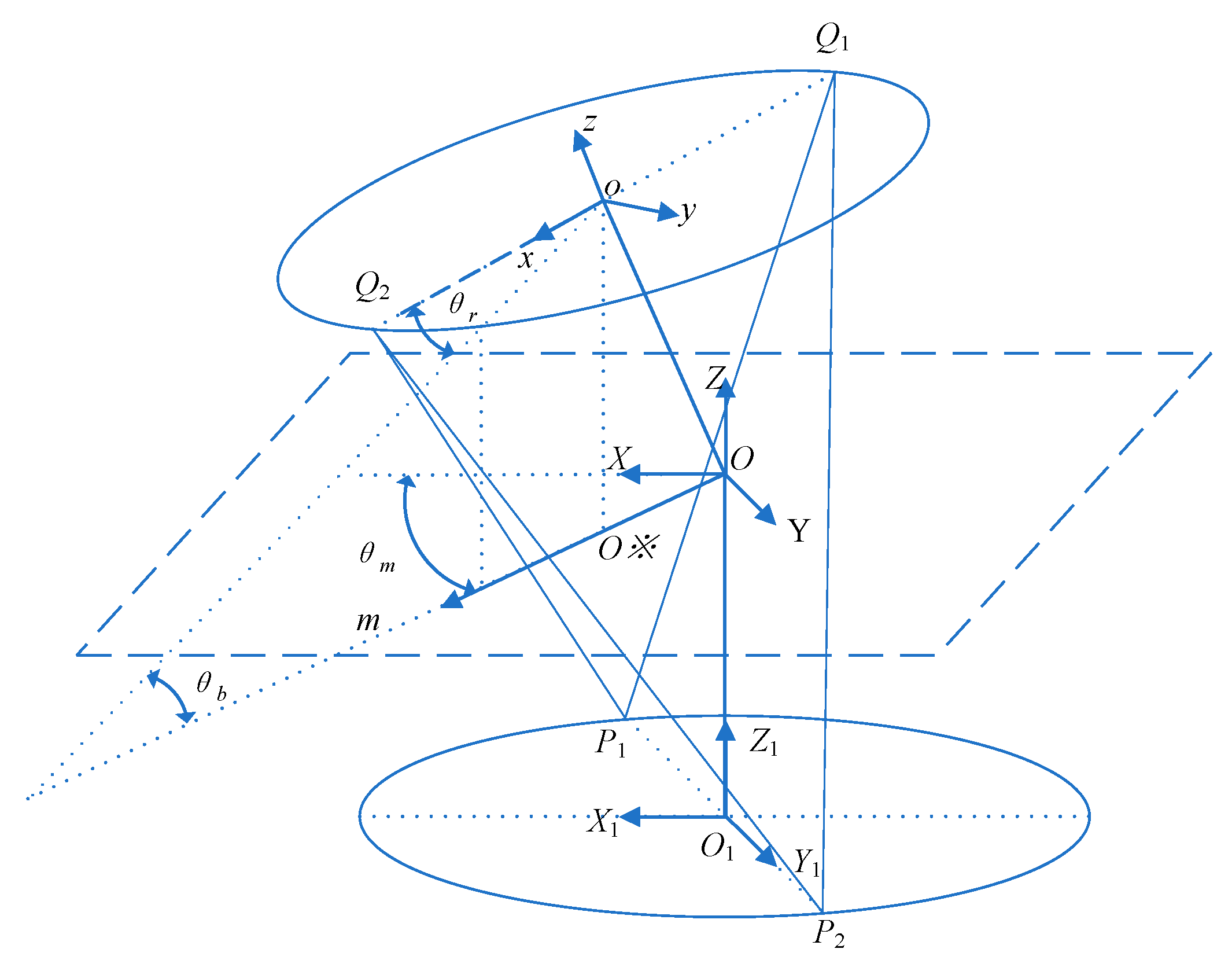
The upper platform’s motion is described by three angles: θ_m (the angle between o’O and OX-axis, representing bending direction), θ_b (the angle between OXY plane and upper platform, representing bending magnitude), and θ_r (the counterclockwise rotation angle about the z-axis, representing yaw angle in the local frame). Here, o’ represents the projection of point o onto the OXY plane. Using Rodrigues’ rotation formula, the rotation matrix R from local to global coordinates is obtained, and the transformation matrix R_h is defined as follows:

$$\begin{array}{l}\mathit{R}=e^{\widehat{\mathit{i}}{\theta }_b}=\mathit{I}+\widehat{\mathit{i}}\sin {\theta }_b+{\widehat{\mathit{i}}}^2(1-\cos {\theta }_b)\\ {\mathit{R}}_h=\left[\begin{array}{cc}\mathit{R}& \mathrm{O}\\ \mathrm{O}& 1\end{array}\right]\end{array}$$

(2)

The specific elements in the equation are as follows:

$$\mathit{i}={\left[-\sin {\theta }_m,\cos {\theta }_m,0\right]}^{\mathrm{T}}$$

(3)

$$\widehat{\mathit{i}}=\left[\begin{array}{ccc}0& 0& \cos {\theta }_m\\ 0& 0& \sin {\theta }_m\\ -\cos {\theta }_m& -\sin {\theta }_m& 0\end{array}\right]$$

(4)

The rotation matrix M_{rot_oz} about the z-axis is given by:

$${\mathit{M}}_{rot\_oz}=\left[\begin{array}{cccc}\cos {\theta }_r& -\sin {\theta }_r& 0& 0\\ \sin {\theta }_r& \cos {\theta }_r& 0& 0\\ 0& 0& 1& 0\\ 0& 0& 0& 1\end{array}\right]$$

(5)

The translation matrix M_trans along the z-axis is given by:

$${\mathit{M}}_{trans}=\left[\begin{array}{cccc}1& 0& 0& 0\\ 0& 1& 0& 0\\ 0& 0& 1& d_2\\ 0& 0& 0& 1\end{array}\right]$$

(6)

Finally, the transformation matrix ^OT_o from the local coordinate system to the global coordinate system is

$${}^O\mathit{T}_o={\mathit{R}}_h{\mathit{M}}_{trans}{\mathit{M}}_{rot\_oz}=\left[\begin{array}{cc}{R}_{O_1{o}_1}& P_{O_1{o}_1}\\ 0& 1\end{array}\right]$$

(7)

Similarly, a transformation matrix from o₁ to C is established. Since there is only a translational relationship rather than a rotational relationship between them, the transformation matrix is

$${}^{o_1}\mathit{T}_C=M_{trans2}=\left[\begin{array}{cc}I& P_{o_{1}C}\\ 0& 1\end{array}\right]$$

(8)

Similarly, the transformation matrix from C to O₂ is derived. Given the presence of both a rotational relationship (with a rotation angle of α) and a translational relationship between them, the transformation matrix is therefore:

$${}^C\mathit{T}_{O_2}=M_{trans3}{M}_{rot.ox}=\left[\begin{array}{cc}{R}_{o_{1}C}& P_{o_{1}C}\\ 0& 1\end{array}\right]$$

(9)

Similarly, the transformation matrix from O₂ to o₂ is derived. Given that the upper and lower joint components are identical, the entire derivation process and matrix structure are exactly the same as those of the O to o matrix. Therefore, the result is

$${}^{O_2}\mathit{T}_{o_2}={\mathit{R}}_h{\mathit{M}}_{trans}{\mathit{M}}_{rot\_oz}=\left[\begin{array}{cc}{R}_{O_2{o}_2}& P_{O_2{o}_2}\\ 0& 1\end{array}\right]$$

(10)

Then, the transformation matrix from the base coordinate system to the end-effector coordinate system of the mechanical arm is

$${}^{O_1}T_{o_2}={}^{O_1}T_{o_2}{}^{o_1}T_C{}^{C}T_{O_2}{}^{O_2}T_{o_2}$$

(11)

For the shoulder joint and wrist joint with the same structure, we marked them as part I and part II, as shown in Figure 4. The physical quantities corresponding to Part I and Part II are represented by subscript 1 and subscript 2, respectively. Since the total transformation matrix is composed of the multiplication of these four transformation matrices, it contains a total of seven variables: the three pose angles of the first joint (θ_m1, θ_r1, θ_b1), the rotation angle α of the intermediate elbow joint, and the three pose angles of the second joint (θ_m2, θ_r2, θ_b2). The relationships between these seven variables and the lengths of the 10 driving cables of the mechanical arm are as follows:

$$\begin{array}{l}{l}_1=\sqrt{(h-0.5d){\sin }^2{\theta }_{b_1}+(dh-0.5d^2)\sin {\theta }_{b_1}\sin {\theta }_{m_1}+0.25d^2+{((h+0.5d)\cos {\theta }_{b_1}+h)}^2}\\ l_2=\sqrt{(h-0.5d){\sin }^2{\theta }_{b_1}+(-dh+0.5d^2)\sin {\theta }_{b_1}\sin {\theta }_{m_1}+0.25d^2+{((h+0.5d)\cos {\theta }_{b_1}+h)}^2}\\ l_3=\sqrt{(h+0.5d){\sin }^2{\theta }_{b_1}+(-dh-0.5d^2)\sin {\theta }_{b_1}\sin {\theta }_{m_1}+0.25d^2+{((h-0.5d)\cos {\theta }_{b_1}+h)}^2}\\ l_4=\sqrt{(h+0.5d){\sin }^2{\theta }_{b_1}+(dh+0.5d^2)\sin {\theta }_{b_1}\sin {\theta }_{m_1}+0.25d^2+{((h-0.5d)\cos {\theta }_{b_1}+h)}^2}\\ l_5=l_{50}+\sqrt{k_1^2+k_2^2+2k_1{k}_2\sin \alpha }-\sqrt{k_1^2+k_2^2}\\ l_6=l_{60}+\sqrt{k_1^2+k_2^2-2k_1{k}_2\sin \alpha }-\sqrt{k_1^2+k_2^2}\\ l_7=2h+2l+\sqrt{(h-0.5d){\sin }^2{\theta }_{b_2}+(dh-0.5d^2)\sin {\theta }_{b_2}\sin {\theta }_{m_2}+0.25d^2+{((h+0.5d)\cos {\theta }_{b_2}+h)}^2}\\ l_8=2h+2l+\sqrt{(h-0.5d){\sin }^2{\theta }_{b_2}+(-dh+0.5d^2)\sin {\theta }_{b_2}\sin {\theta }_{m_2}+0.25d^2+{((h+0.5d)\cos {\theta }_{b_2}+h)}^2}\\ l_9=2h+2l+\sqrt{(h+0.5d){\sin }^2{\theta }_{b_2}+(-dh-0.5d^2)\sin {\theta }_{b_2}\sin {\theta }_{m_2}+0.25d^2+{((h-0.5d)\cos {\theta }_{b_2}+h)}^2}\\ l_{10}=2h+2l+\sqrt{(h+0.5d){\sin }^2{\theta }_{b_2}+(dh+0.5d^2)\sin {\theta }_{b_2}\sin {\theta }_{m_2}+0.25d^2+{((h-0.5d)\cos {\theta }_{b_2}+h)}^2}\end{array}$$

(12)

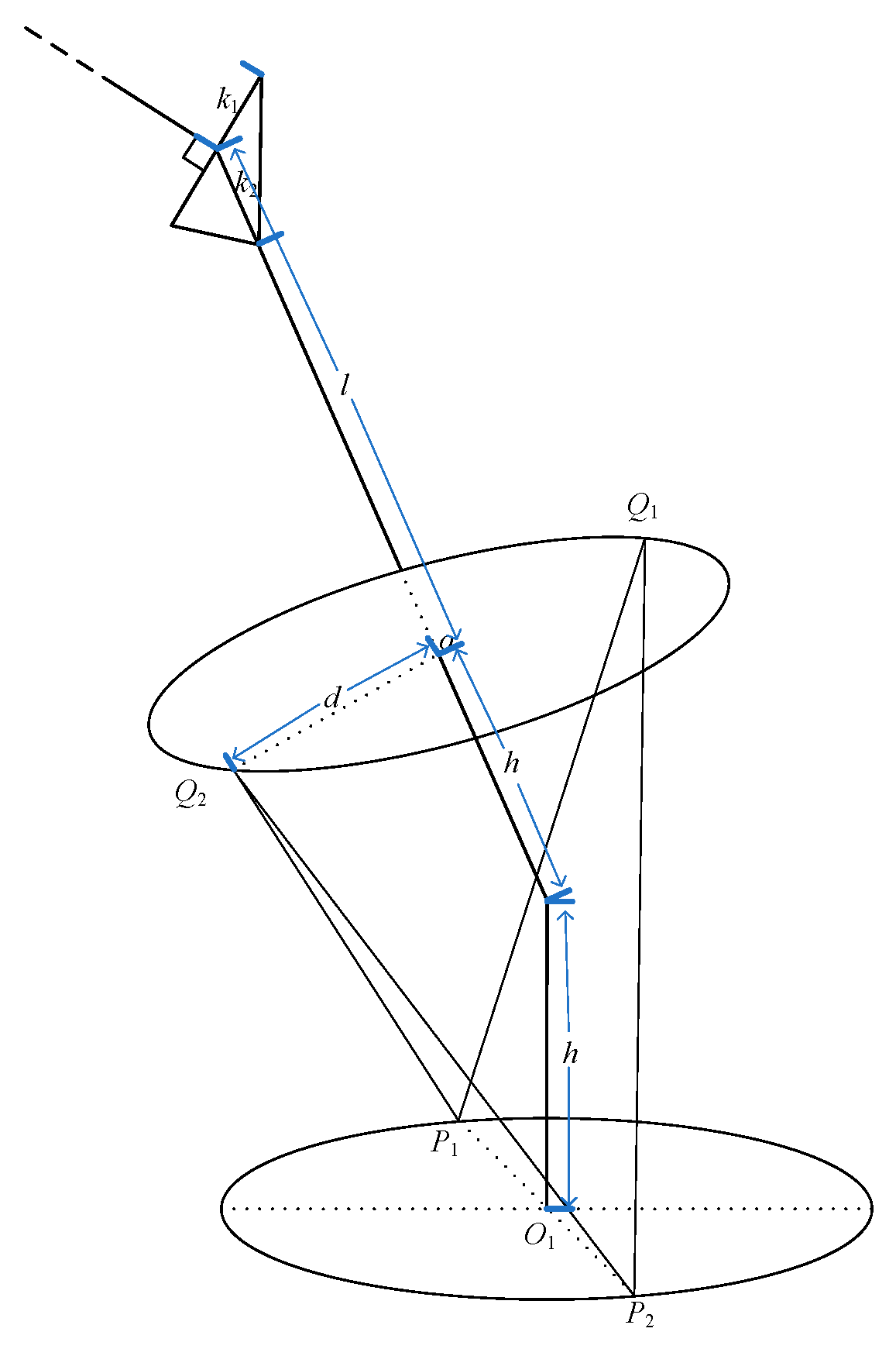
Here, l_i (i = 1, 2, …, 10) denotes the lengths of the ten driving cables. k₁ and k₂ represent the length of the elbow cable bracket and the length of the intermediate link, respectively, as illustrated in Figure 6.

Among them are h = 15 cm, d = 10 cm, k₁ = 5 cm, k₂ = 10 cm, and l = 50 cm. In practical applications, the dimensional parameters of the manipulator can be appropriately adjusted to adapt to the requirements of the working environment.

3.2. Inverse Kinematics

Given that the self-insulated mechanical arm designed in the manuscript has seven degrees of freedom, a hierarchical control strategy is adopted to avoid the multi-solution problem of joint angles. Specifically, the control process first determines the position of joint point C and then calculates the pose of the end-effector. This approach decomposes the 7-DOF mechanical arm into upper and lower parts, solving the inverse kinematics sequentially. Such a solution method not only eliminates redundant joint configurations but also prevents collisions between the arm’s components.

Therefore, the inverse kinematics of the lower arm segment is first solved starting from joint C. Specifically, given the coordinates of C as [x_C y_C z_C]^T, the pose angles θ_m2, θ_r2, and θ_b2 are derived. The results are as follows:

$$\begin{array}{l}{\theta }_{m_1}=\arctan \left({\displaystyle \frac{y_C}{x_C}}\right)\\ {\theta }_{r_1}=\phi \\ {\theta }_{b_1}=\arctan \left({\displaystyle \frac{\sqrt{x_C^2+y_C^2}}{z_C-h}}\right)\end{array}$$

(13)

The specification of the angle φ does not affect the coordinate position of joint C, and the values of the elbow joint rotation angle α and angle φ are designated in the first control step. Therefore, in the inverse kinematics solution of the lower self-insulated joint segment in the second step, the coordinate position of the self-insulated joint is already determined, requiring only the same inverse kinematic solution process. The results are as follows:

$$\begin{array}{l}{\theta }_{m_2}=\arctan \left({\displaystyle \frac{y_{pr}^{\prime }}{x_{pr}^{\prime }}}\right)\\ {\theta }_{r_2}=\psi \\ {\theta }_{b_2}=\arctan \left[{\displaystyle \frac{\sqrt{{(x_{pr}^{\prime })}^2+{(y_{pr}^{\prime })}^2}}{z_{pr}^{\prime }-h}}\right]\end{array}$$

(14)

Here, [x_pr y_pr z_pr]^T is known as the end-coordinate of the sensor probe in the world coordinate system. The angle ψ is arbitrarily specified, influencing neither the mechanical arm’s state and pose nor its kinematic configuration, but only the orientation of the sensor probe. The coordinates [x’_pr y’_pr z’_pr]^T, representing the probe’s position in the elbow joint coordinate system, are calculated as follows:

$$R_{O_1{o}_1}^{-1}{R}_C^{-1}\left[\begin{array}{c}{x}_{pr}\\ y_{pr}\\ z_{pr}\end{array}\right]=\left[\begin{array}{c}{x}_{pr}^{\prime }\\ y_{pr}^{\prime }\\ z_{pr}^{\prime }\end{array}\right]$$

(15)

3.3. Static Modeling

After completing the kinematic modeling, this manuscript conducts static modeling of the mechanical arm to verify its behavior when the end-effector is disturbed by a heavy load. First, the relationship between the rotation angles and the end-probe coordinates is established through transformation matrices:

$${}^{O_1}T_{o_1}{}^{o_1}T_C{}^{C}T_{O_2}{}^{O_2}T_{o_1}\left[\begin{array}{c}0\\ 0\\ H\\ 1\end{array}\right]=\left[\begin{array}{c}{x}_{pr}\\ y_{pr}\\ z_{pr}\\ 1\end{array}\right]$$

(16)

By taking the derivative of both sides, a Jacobian matrix is established, yielding

$$\left[\begin{array}{c}{\dot{x}}_{pr}\\ {\dot{y}}_{pr}\\ {\dot{z}}_{pr}\end{array}\right]=\left[\begin{array}{c}\begin{array}{cccc}{J}_{11}& J_{12}& \dots & J_{17}\end{array}\\ \begin{array}{cccc}{J}_{21}& J_{22}& \dots & J_{27}\end{array}\\ \begin{array}{cccc}{J}_{31}& J_{32}& \dots & J_{37}\end{array}\end{array}\right]\left[\begin{array}{c}\begin{array}{c}{\dot{\theta }}_{m_1}\\ {\dot{\theta }}_{r_1}\\ {\dot{\theta }}_{b_1}\end{array}\\ \begin{array}{c}\alpha \\ {\dot{\theta }}_{m_2}\\ {\dot{\theta }}_{r_2}\\ {\dot{\theta }}_{b_2}\end{array}\end{array}\right]$$

(17)

The Jacobian matrix is a three-row-seven-column matrix with rank (J) = 3. Its pseudo-inverse matrix is given by

$$J^{+}=J^{\mathrm{T}}{(J{J}^{\mathrm{T}})}^{-1}$$

(18)

Thus, the transformation relationship between the torques corresponding to each rotation angle and the end-effector output force is obtained, where [F_x F_y F_z]^T is the external force on the end, and [τ_m1 τ_r1 τ_b1 τ_α τ_m2 τ_r2 τ_b2]^T is the equivalent moment of each joint angle:

$$\left[\begin{array}{c}{F}_x\\ F_y\\ F_z\end{array}\right]={(J^{+})}^T\left[\begin{array}{c}{\tau }_{m_1}\\ {\tau }_{r_1}\\ {\tau }_{b_1}\\ {\tau }_{\alpha }\\ {\tau }_{m_2}\\ {\tau }_{r_2}\\ {\tau }_{b_2}\end{array}\right]$$

(19)

Furthermore, based on the established kinematic relationships, the relationship between the tension provided by the mechanical arm’s driving cables F_li(i = 1, 2, …, 10) and the torque at each corresponding rotation angle is as follows:

$$\begin{array}{c}{\tau }_{m_1}=\sqrt{h^2+0.25d^2}\sin \left({\theta }_{b_1}+\arctan {\displaystyle \frac{d}{2h}}\right)\cdot {\displaystyle \frac{\sqrt{0.5d^2(1-\sin {\theta }_{b_1})}}{l_1}}{F}_{l_1}\\ \hspace{0.5em}\hspace{0.5em}-\sqrt{h^2+0.25d^2}\sin \left({\theta }_{b_1}+\arctan {\displaystyle \frac{d}{2h}}\right)\cdot {\displaystyle \frac{\sqrt{0.5d^2(1+\sin {\theta }_{b_1})}}{l_2}}{F}_{l_2}\\ \hspace{0.5em}\hspace{0.5em}+\sqrt{h^2+0.25d^2}\sin \left(\arctan {\displaystyle \frac{d}{2h}}-{\theta }_{b_1}\right)\cdot {\displaystyle \frac{\sqrt{0.5d^2(1-\sin {\theta }_{b_1})}}{l_3}}{F}_{l_3}\\ \hspace{0.5em}\hspace{0.5em}-\sqrt{h^2+0.25d^2}\sin \left(\arctan {\displaystyle \frac{d}{2h}}-{\theta }_{b_1}\right)\cdot {\displaystyle \frac{\sqrt{0.5d^2(1+\sin {\theta }_{b_1})}}{l_4}}{F}_{l_4}\end{array}$$

(20)

$${\tau }_{r_1}=0.707d{F}_{l_1}-0.707d{F}_{l_2}+0.707d{F}_{l_3}-0.707d{F}_{l_4}$$

(21)

$$\begin{array}{c}{\tau }_{b_1}=\left[\sqrt{h^2+0.25d^2}\cos \left({\theta }_{b_1}+\arctan {\displaystyle \frac{d}{2h}}\right)+h\right]\cdot {\displaystyle \frac{\sqrt{l_1^2-0.5d^2(1-\sin {\theta }_{b_1})}}{l_1}}{F}_{l_1}\\ \hspace{0.5em}\hspace{0.5em}+\left[\sqrt{h^2+0.25d^2}\cos \left({\theta }_{b_1}+\arctan {\displaystyle \frac{d}{2h}}\right)+h\right]\cdot {\displaystyle \frac{\sqrt{l_2^2-0.5d^2(1-\sin {\theta }_{b_1})}}{l_2}}{F}_{l_1}\\ \hspace{0.5em}\hspace{0.5em}-\left[\sqrt{h^2+0.25d^2}\cos \left(\arctan {\displaystyle \frac{d}{2h}}-{\theta }_{b_1}\right)+h\right]\cdot {\displaystyle \frac{\sqrt{l_3^2-0.5d^2(1-\sin {\theta }_{b_1})}}{l_3}}{F}_{l_3}\\ \hspace{0.5em}\hspace{0.5em}-\left[\sqrt{h^2+0.25d^2}\cos \left(\arctan {\displaystyle \frac{d}{2h}}-{\theta }_{b_1}\right)+h\right]\cdot {\displaystyle \frac{\sqrt{l_4^2-0.5d^2(1-\sin {\theta }_{b_1})}}{l_4}}{F}_{l_4}\end{array}$$

(22)

$${\tau }_{\alpha }={\displaystyle \frac{k_1{k}_2}{l_5}}\cos \alpha F_{l_5}-{\displaystyle \frac{k_1{k}_1}{l_6}}\cos \alpha F_{l_6}$$

(23)

$$\begin{array}{c}{\tau }_{m_2}=\sqrt{h^2+0.25d^2}\sin \left({\theta }_{b_2}+\arctan {\displaystyle \frac{d}{2h}}\right)\cdot {\displaystyle \frac{\sqrt{0.5d^2(1-\sin {\theta }_{b_2})}}{l_7-l_{70}}}{F}_{l_7}\\ \hspace{0.5em}\hspace{0.5em}-\sqrt{h^2+0.25d^2}\sin \left({\theta }_{b_2}+\arctan {\displaystyle \frac{d}{2h}}\right)\cdot {\displaystyle \frac{\sqrt{0.5d^2(1+\sin {\theta }_{b_2})}}{l_8-l_{80}}}{F}_{l_8}\\ \hspace{0.5em}\hspace{0.5em}+\sqrt{h^2+0.25d^2}\sin \left(\arctan {\displaystyle \frac{d}{2h}}-{\theta }_{b_2}\right)\cdot {\displaystyle \frac{\sqrt{0.5d^2(1-\sin {\theta }_{b_2})}}{l_9-l_{90}}}{F}_{l_9}\\ \hspace{0.5em}\hspace{0.5em}-\sqrt{h^2+0.25d^2}\sin \left(\arctan {\displaystyle \frac{d}{2h}}-{\theta }_{b_2}\right)\cdot {\displaystyle \frac{\sqrt{0.5d^2(1+\sin {\theta }_{b_2})}}{l_{10}-l_{100}}}{F}_{l_{10}}\end{array}$$

(24)

$${\tau }_{r_2}=0.707d{F}_{l_7}-0.707d{F}_{l_8}+0.707d{F}_{l_9}-0.707d{F}_{l_{10}}$$

(25)

$$\begin{array}{c}{\tau }_{b_2}=\left[\sqrt{h^2+0.25d^2}\cos \left({\theta }_{b_2}+\arctan {\displaystyle \frac{d}{2h}}\right)+h\right]\cdot {\displaystyle \frac{\sqrt{{(l_7-l_{70})}^2-0.5d^2(1-\sin {\theta }_{b_2})}}{l_7-l_{70}}}{F}_{l_7}\\ \hspace{0.5em}\hspace{0.5em}+\left[\sqrt{h^2+0.25d^2}\cos \left({\theta }_{b_2}+\arctan {\displaystyle \frac{d}{2h}}\right)+h\right]\cdot {\displaystyle \frac{\sqrt{{(l_8-l_{80})}^2-0.5d^2(1-\sin {\theta }_{b_2})}}{l_8-l_{80}}}{F}_{l_8}\\ \hspace{0.5em}\hspace{0.5em}-\left[\sqrt{h^2+0.25d^2}\cos \left(\arctan {\displaystyle \frac{d}{2h}}-{\theta }_{b_2}\right)+h\right]\cdot {\displaystyle \frac{\sqrt{{(l_9-l_{90})}^2-0.5d^2(1-\sin {\theta }_{b_2})}}{l_9-l_{90}}}{F}_{l_9}\\ \hspace{0.5em}\hspace{0.5em}\hspace{0.5em}\hspace{0.5em}-\left[\sqrt{h^2+0.25d^2}\cos \left(\arctan {\displaystyle \frac{d}{2h}}-{\theta }_{b_2}\right)+h\right]\cdot {\displaystyle \frac{\sqrt{{(l_{10}-l_{100})}^2-0.5d^2(1-\sin {\theta }_{b_2})}}{l_{10}-l_{100}}}{F}_{l_{10}}\end{array}$$

(26)

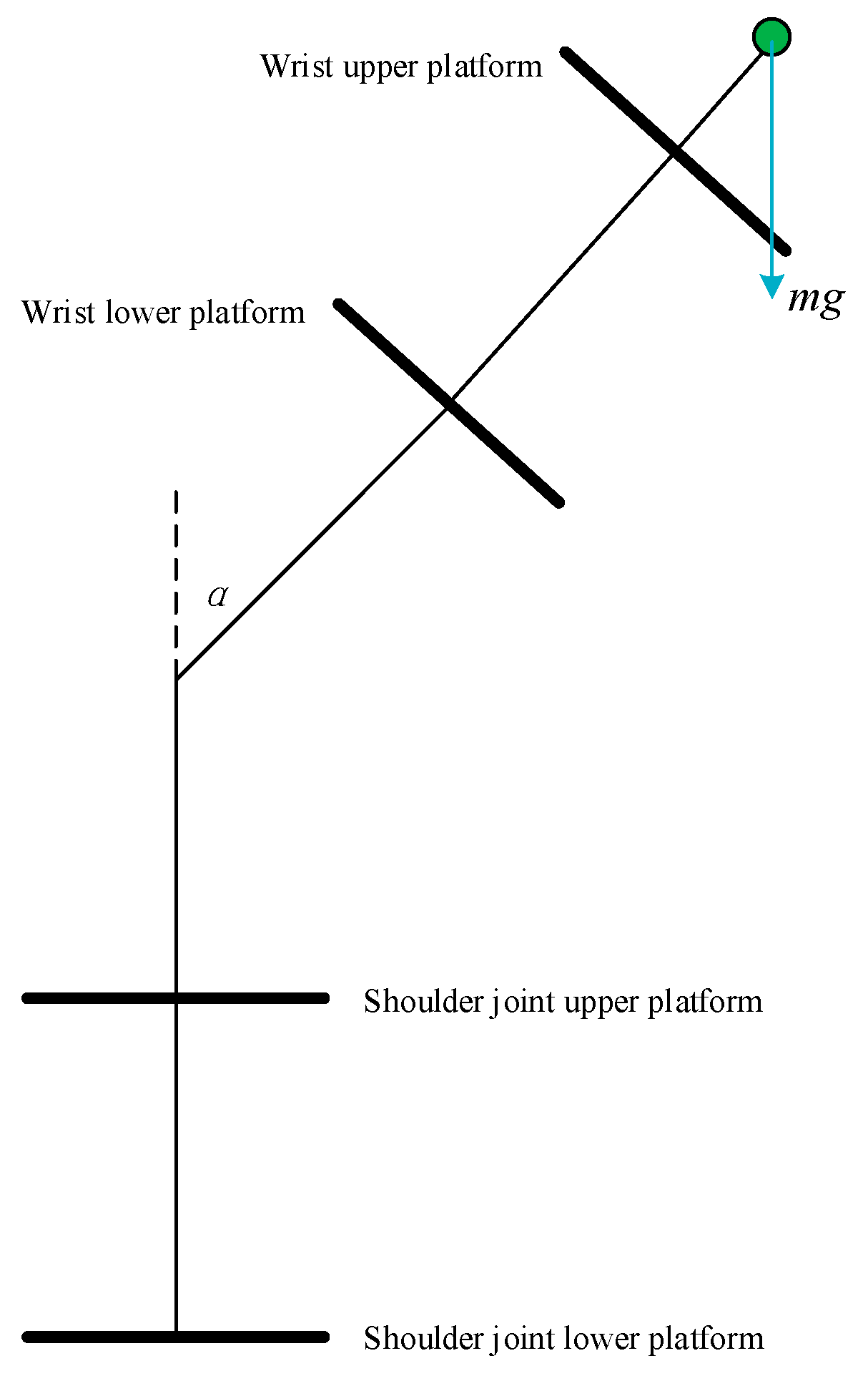
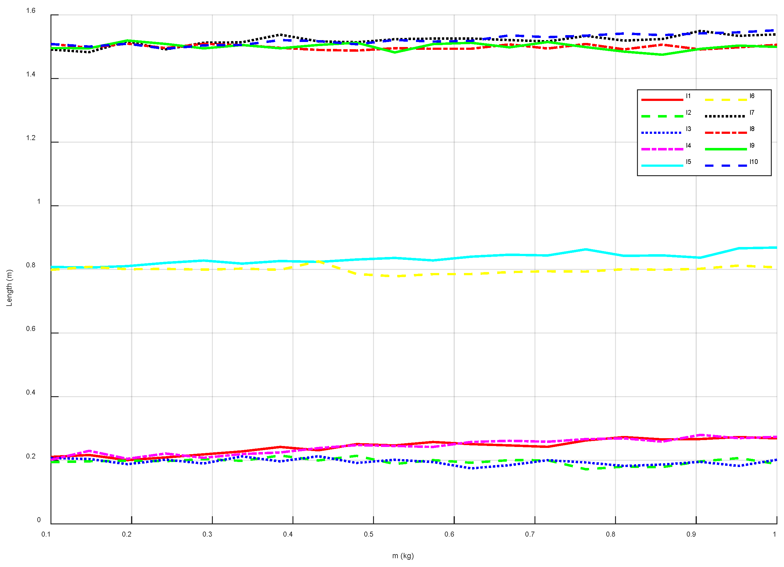
The cable stretching deformation of the mechanical arm is simulated at joint angles ${\left[\begin{array}{ccccccc}0& 0& 0& \frac{\pi }{3}& 0& 0& 0\end{array}\right]}^T$ when an additional mass-load m is applied to the end-effector, as illustrated in Figure 7.

Here, the cables are modeled as springs with a large elastic modulus, where the spring constant is set to 1000 N/m. By varying the end-load from 0.1 kg to 1 kg, the variation curves of the driving cable lengths are obtained, as shown in Figure 8.

4. Workspace Simulation

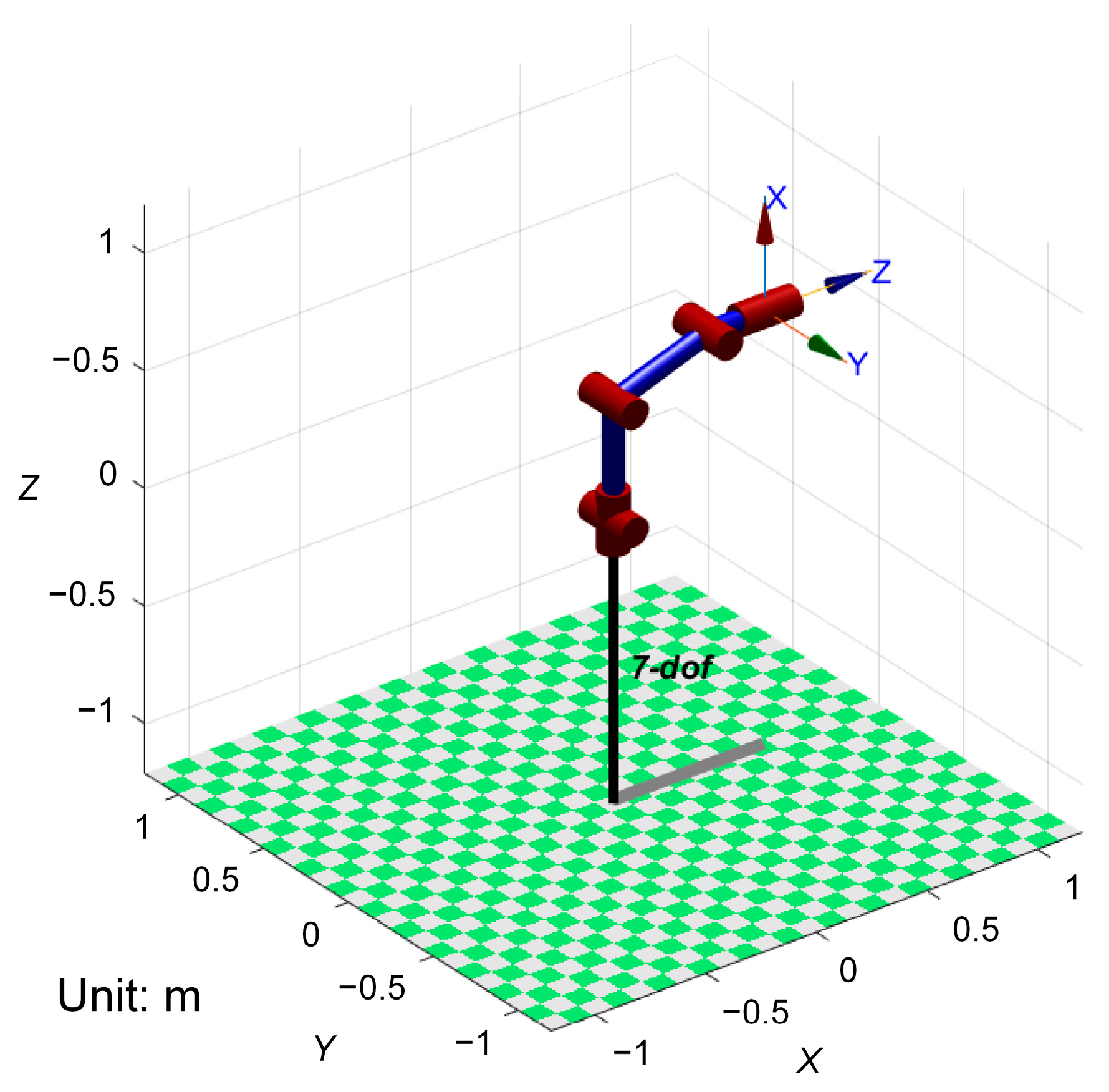
According to the self-insulating bionic joint design described above and the overall mechanical design of the mechanical arm, a simulation environment of the mechanical arm end workspace is built to verify the working adaptability of the bionic self-insulating mechanical arm in the hidden space environment of the cable tunnel. As shown in Figure 9, an equivalent simulation model of the mechanical arm is built.

The main dimensions of the robot arm used in the simulation are set to l = 65 cm, h = 15 cm. The joint rotation angle α is limited to between 110° and −110°. The angle θ_m2 is limited to between −60° and 60°. The angle θ_r2 is limited to between −60° and 60°. The angle θ_b2 is limited to between −60° and 60°.

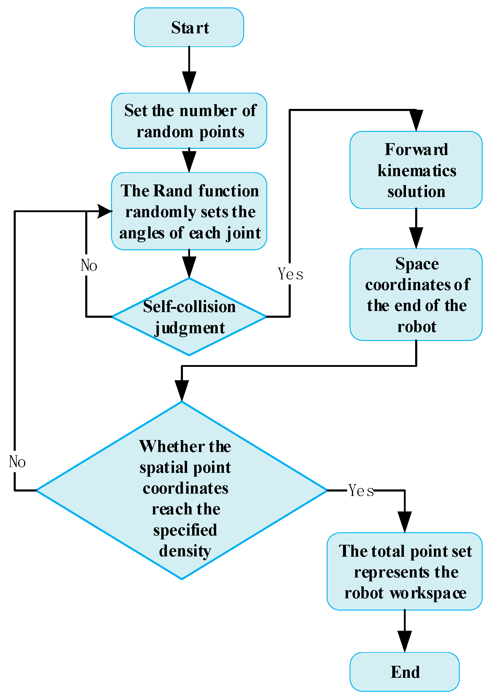
The Monte Carlo method is used in MATLAB R2024b to simulate its workspace. The Monte Carlo method is used to generate joint working angle groups. Its flow chart is shown in Figure 10.

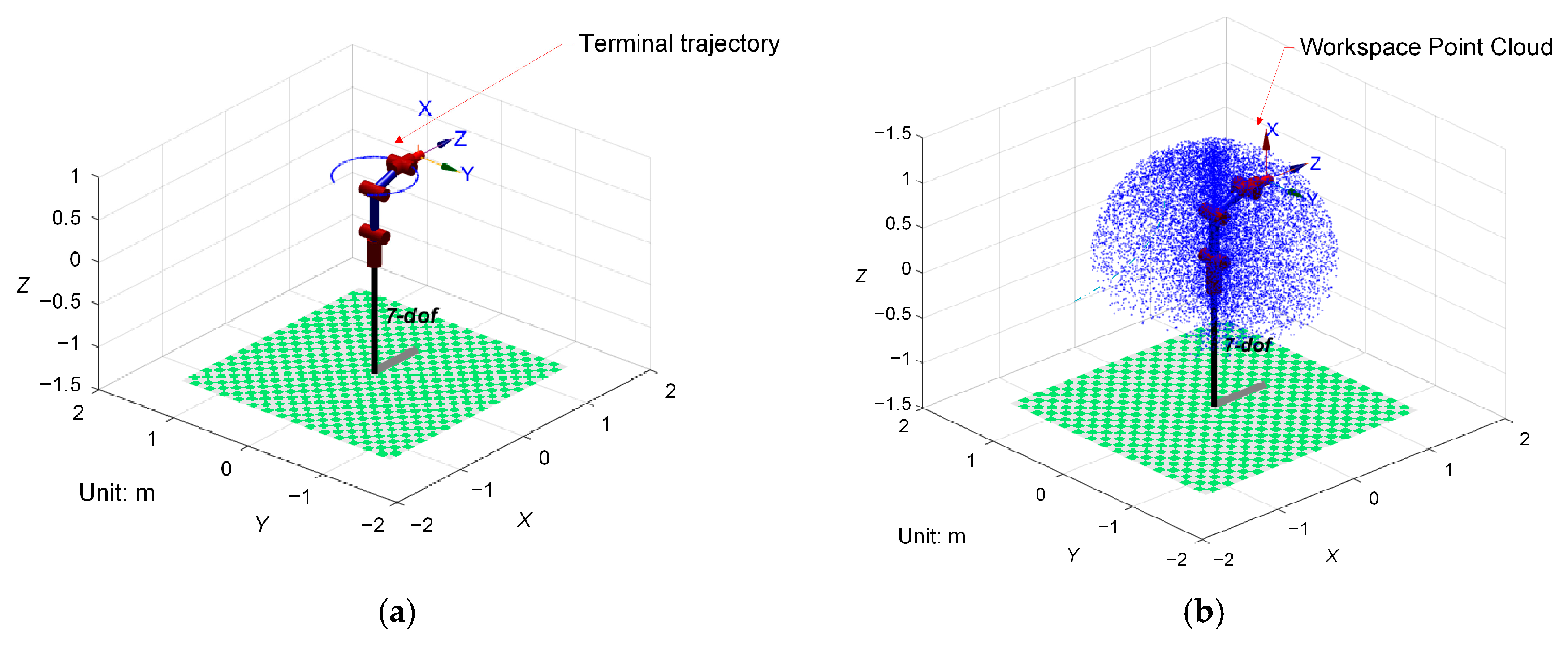
In the process of randomly generating angle groups within the joint working angle range, the mechanical arm self-collision judgment condition is added to discard the unusable angle groups. The generated usable angle groups are used to generate the space coordinate points of the mechanical arm end through the forward kinematics solution process established in the previous article. The generation of space coordinate points stops when a certain density requirement is reached, and finally a workspace point set is formed. During the generation process, the end working coordinates are calibrated and recorded. The generation process is shown in Figure 11a,b.

The mechanical arm’s three-dimensional workspace exhibits a hemispheroidal configuration, as illustrated by the generated point cloud in Figure 11b.

At the same time, this paper generates uniformly distributed joint angle combinations within the range of the robot joint angle limit. The position of the end effector is calculated for each set of joint angles (positive kinematics), and the Yoshikawa operability index is calculated based on the position Jacobian matrix J_pose:

$$\omega =\sqrt{\det (J_{pose}{J}_{pose}^T)}$$

(27)

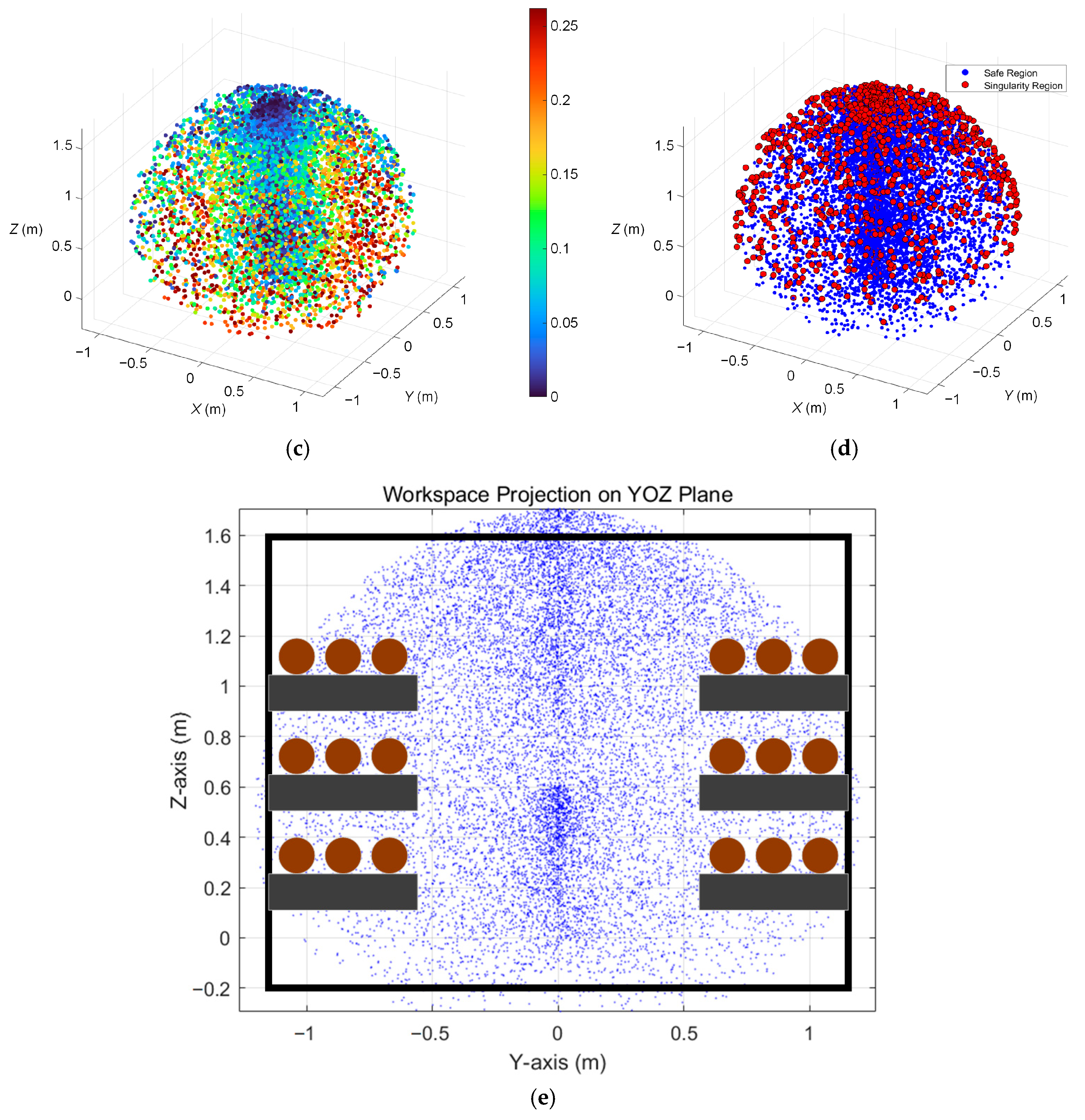
This indicator reflects the flexibility of the end effector at the current position. The larger the value, the stronger the operability. The results are presented in the form of a heat map, as shown in Figure 11c. The high operability area is mainly distributed in the middle workspace of the robot arm, mainly corresponding to the situation when the elbow joint is at an intermediate angle and the Jacobian matrix condition number is small. The low operability area appears at the edge of the workspace, especially when each joint is close to the extreme angle, and the robot arm is close to kinematic singularity.

Regarding the singularity of the robot arm, this paper performs singular value decomposition (SVD) on the Jacobian matrix and extracts the minimum singular value σ_min. The threshold σ_min < 0.06 is defined as the singular region, and the robot arm is judged to be in a singular configuration, and the rest is the normal region. The analysis results are shown in Figure 11d. Singular region (red point): It appears in two typical configurations, one is the elbow joint straight, and the other is the upper and lower shoulder joints and wrist joints are aligned, that is, when the axis coincides. In the safe area, the robot arm has high motion stability. As can be seen from the results, high maneuverability areas are usually far away from singular configurations. In practical applications, trajectory planning should avoid crossing red singular areas or reduce the motion speed nearby.

Projection of this workspace point cloud onto the yoz plane enables comparative analysis with the cross-sectional profile of the concealed cable tunnel, presented in Figure 11e. The cross-sectional workspace approximates an oblate ellipsoid with minor and major axes measuring 1.25 m and 1.65 m, respectively. This spatial configuration demonstrates sufficient coverage capability for inspection tasks within the cable tunnel’s 2.5 m (length) × 1.8 m (height) cross-sectional area, ensuring comprehensive access to all cable inspection zones. These findings verify that the mechanical arm’s operational workspace fully satisfies the detection requirements for cables in concealed spaces.

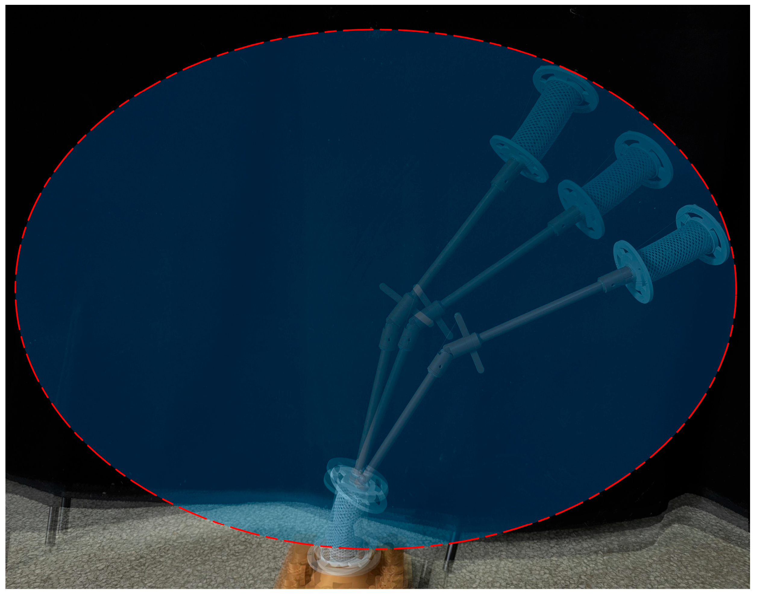
Through comparative analysis of the workspace accessibility of the mechanical arm experimental model, as shown in Figure 12, the simulation results basically coincide with the actual working conditions. This phenomenon indicates that the mechanical arm has the capability to cover a quasi-elliptical three-dimensional workspace.

5. Self-Insulation Performance Simulation Analysis

The insulation performance of the flexible joint is the most crucial part along the mechanical arm. In order to examine the electric field strength distribution of the joint under a certain voltage level, this manuscript constructs a finite element model based on the simulation environment. The insulation materials and parameters are set for the mechanical arm components. The simulation diagrams of the potential and electric field distribution in different planes of the mechanical arm under the 220 kV voltage level are given in Figure 10. The material settings of the components are shown in

Table 2. Material selection comparison.

Material	Tensile Strength (MPa)	Flexural Strength (MPa)	Elastic Modulus (GPa)	Density (g/cm3)	Dielectric Strength (kV/mm)	Selection
Epoxy resin	50–120	400–800	2.5–4.5	1.1–1.4	15–22	√
Polyester resin	40–90	180–400	2.0–3.5	1.2–1.4	10–15	√
Phenolic resin	30–60	100–300	2.0–3.0	1.3–1.5	10–15	×
Silicone	10–40	50–150	1.0–2.0	1.1–1.3	15–25	×
Polyimide	70–120	200–500	3.0–5.0	1.4–1.6	20–30	×

. Among them, the center of the bottom surface of the groove of the moving platform and the fixed platform coincides with the center of the bottom surface of itself, and the four openings on the moving platform and the fixed platform are distributed on the platform surface with equal arc lengths.

In this finite element simulation, the mesh density is controlled by the geometric shape of the robot. The minimum mesh size in this simulation model is about 0.005 m, the unit type is tetrahedral unit, and the solver is the built-in Newton iteration solver of COMSOL 6.0.

The materials used in the simulation were selected based on the robotic arm’s recommended specifications. The main structure was constructed using epoxy resin, while the driving tendons were made of polyester fiber. A comparison of their properties with several common materials is presented in Table 2. As shown, epoxy resin exhibits a favorable combination of bending strength, elastic modulus, and density, making it well-suited as a lightweight, self-insulating, and rigid structural material for the robotic arm. On the other hand, polyester fiber, with its relatively low bending strength but high tensile strength, is appropriate for tendon applications. In the finite element simulation of insulation performance, the influence of the insulating tendon material was negligible, and thus, the tendon section was temporarily omitted.

In the selection of materials for the self-insulating rope-driven manipulator working in a live environment, after a comprehensive comparison of the performance of various resin-based materials, it was finally determined that epoxy resin was used as the main material of the manipulator and polyester resin was used as the driving rope material. Epoxy resin has a high tensile strength of 50–120 MPa and an excellent bending strength of 400–800 MPa, which can meet the requirements of the main body of the manipulator for structural strength and durability. At the same time, its elastic modulus of 2.5–4.5 GPa ensures rigidity while avoiding material brittleness. The low density of 1.1–1.4 g/cm³ helps to achieve lightweight design, and the dielectric strength of 15–22 kV/mm ensures sufficient insulation performance. These performance indicators are significantly better than phenolic resin (30–60 MPa tensile, 100–300 MPa bending) and silicone (10–40 MPa tensile, 50–150 MPa bending) and can better meet the requirements of the main body of the manipulator for structural strength. At the same time, the elastic modulus of epoxy resin of 2.5–4.5 GPa ensures sufficient rigidity while avoiding the brittleness problem that may be caused by polyimide (3.0–5.0 GPa), and its density of 1.1–1.4 g/cm³ is also better than polyimide (1.4–1.6 g/cm³), which is more conducive to lightweight design. In terms of insulation performance, the dielectric strength of epoxy resin of 15–22 kV/mm fully meets the working requirements of the charged environment. Although it is slightly lower than that of polyimide (20–30 kV/mm), considering the significantly higher cost of polyimide, epoxy resin has obvious advantages in terms of cost performance.

For the selection of drive rope materials, polyester resin is an ideal choice with its moderate mechanical properties (40–90 MPa tensile strength, 180–400 MPa bending strength) and elastic modulus of 2.0–3.5 GPa. Compared with silicone (1.0–2.0 GPa elastic modulus), polyester resin has better dimensional stability and can transmit driving force more accurately; compared with phenolic resin, polyester resin has better flexibility. Although polyimide is superior in performance, its high cost makes it unsuitable as a rope material that needs to be used in large quantities. Although the dielectric strength of polyester resin of 10–15 kV/mm is not as good as that of epoxy resin and polyimide, it has fully met the insulation requirements of ropes, and its cost advantage is obvious. Considering the performance requirements and economic benefits, the combination of epoxy resin and polyester resin has achieved the best balance in mechanical properties, control accuracy and insulation safety, and is the most suitable material solution for rope-driven manipulators in live environments. Overall, the high strength, high rigidity, and lightweight properties of epoxy resin make it an ideal choice for the main body of the robotic arm, while the moderate elasticity and bending properties of polyester resin make it more suitable as a drive rope material. The combination of the two achieves the best balance in ensuring mechanical properties, control accuracy, and insulation safety.

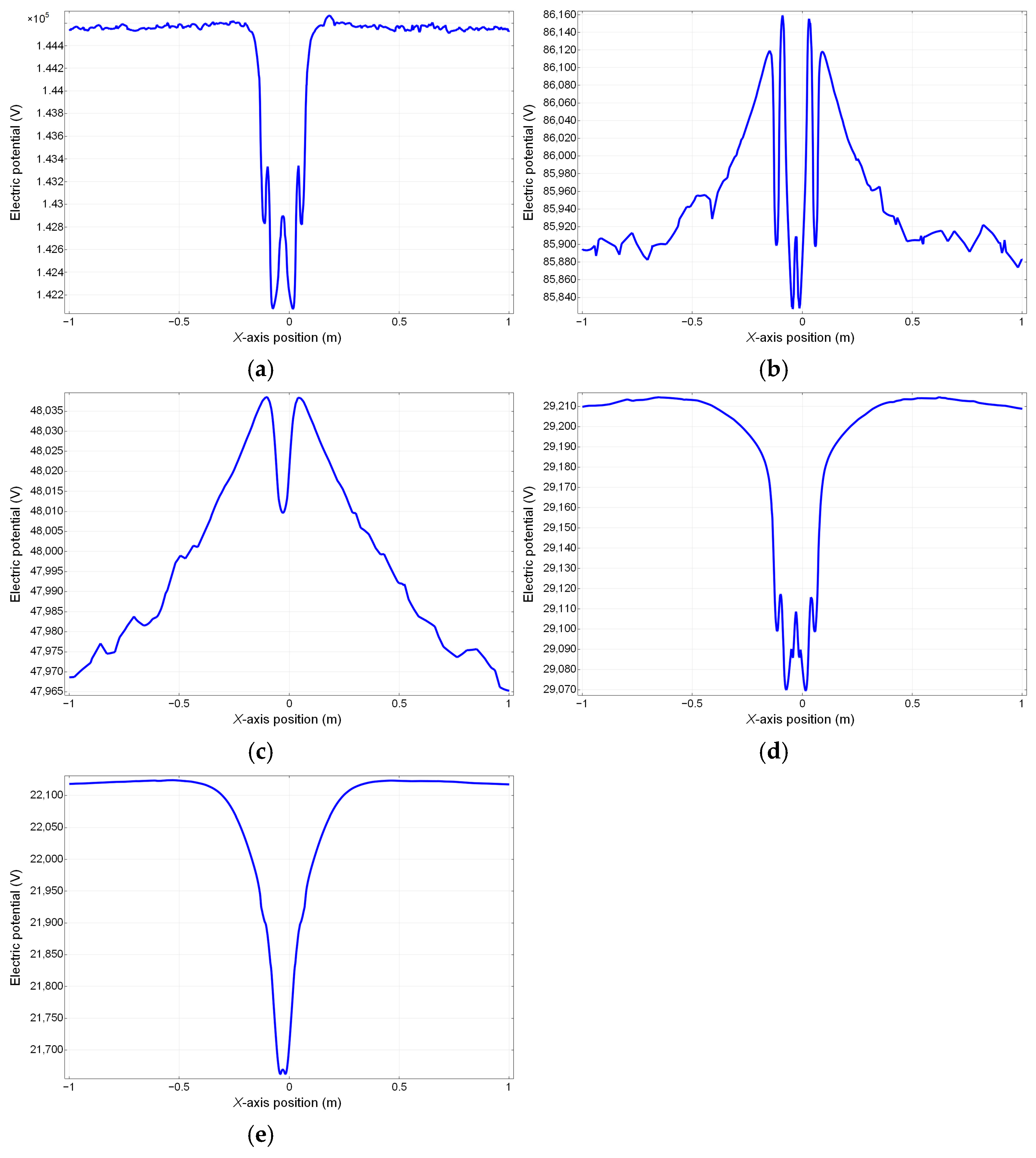
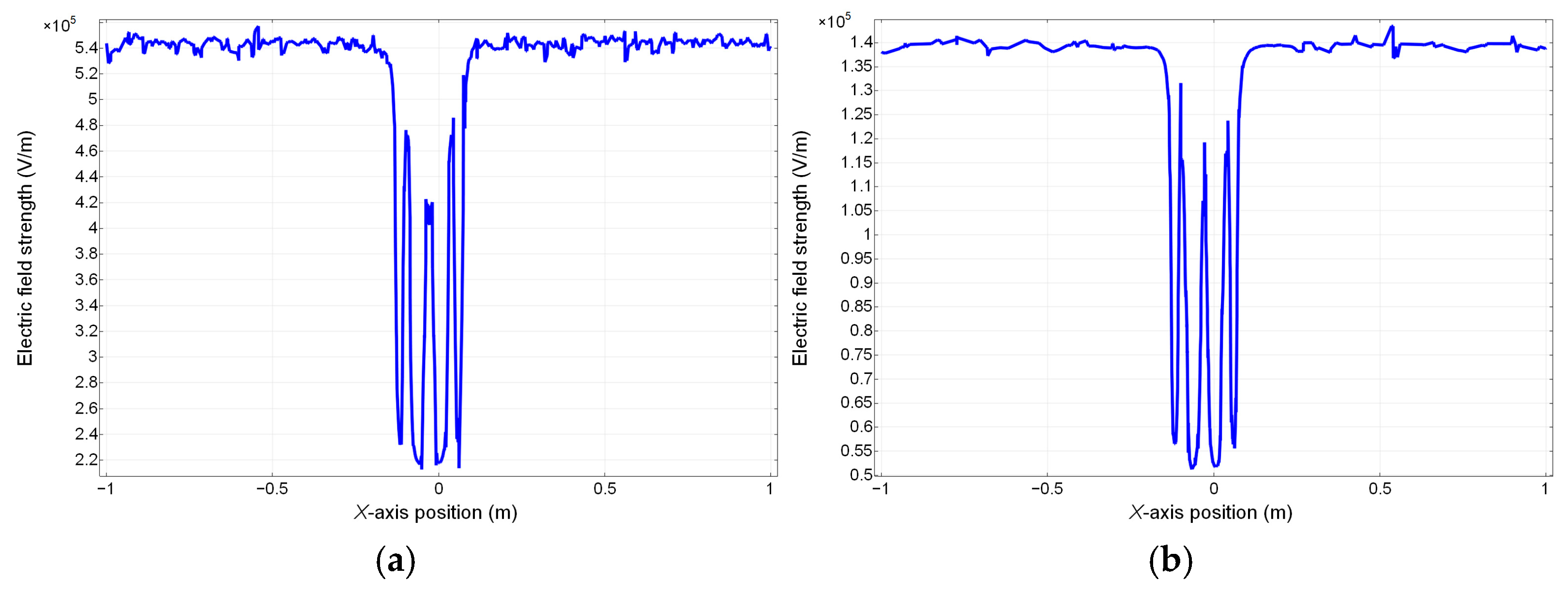
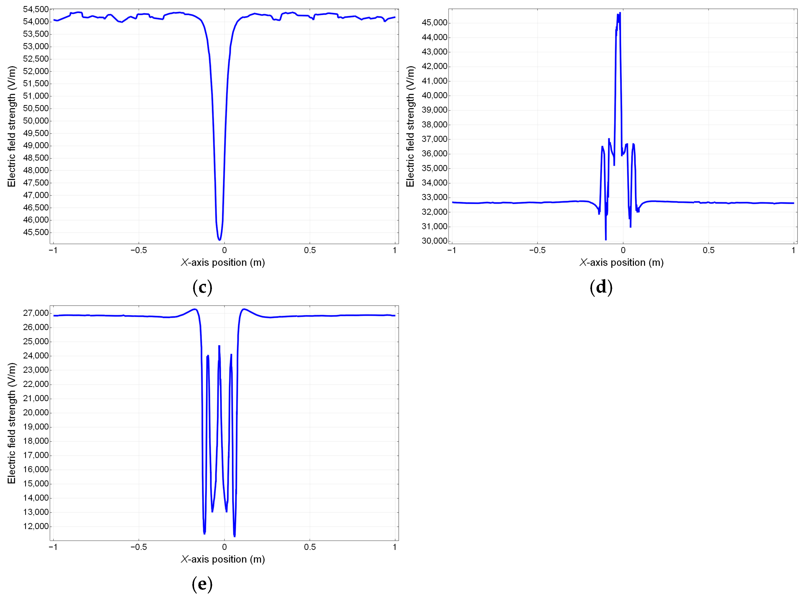
Five planes are selected to calculate the electric field (Figure 13). The field values are calculated along the diameter of the plane. Plane 1 is the moving platform of the wrist joint. Plane 2 is the fixed platform of the wrist joint. Plane 3 is the elbow joint. Plane 4 is the moving platform of the shoulder joint. Plane 5 is the fixed platform of the shoulder joint. The specific simulation environment details are shown in

Table 3. Finite element model material settings.

Item		Technical Detail
Computer workstation parameters	CPU	Intel Core i5-9400
	RAM	24 GB
	ROM	1 TB solid state drive
	Operating system	Windows 11 64-bit
FEM calculation platform	FEM software	COMSOL 6.0
	Used physical field toolbox	Static electricity field toolbox
Simulation model and boundary conditions	Approximation for the infinite boundary	Using a calculation area significantly larger than the mechanical arm
	Geometric shape of the calculation area	Cube (4 × 4 × 4 m)
	High-voltage boundary condition	220 kV at the surface of the cable
	Theoretical infinite boundary condition	0 V at infinity
	Approximate infinite boundary condition	Using a grounding boundary condition (0 V) at the boundary of the calculation area
	Relative permittivity of the mechanical arm	3.2
Meshing method	Mesh density	Ultra fine
	Element type	Tetrahedral
	Element number	1,113,950
	Maximum mesh size	0.13 m
	Minimum mesh size	0.005 m
FEM equation solving	Solver	Nonlinear Newton iteration solver (COMSOL built-in)
	Residual tolerance	0.01
	Maximum number of iterations	10,000

.

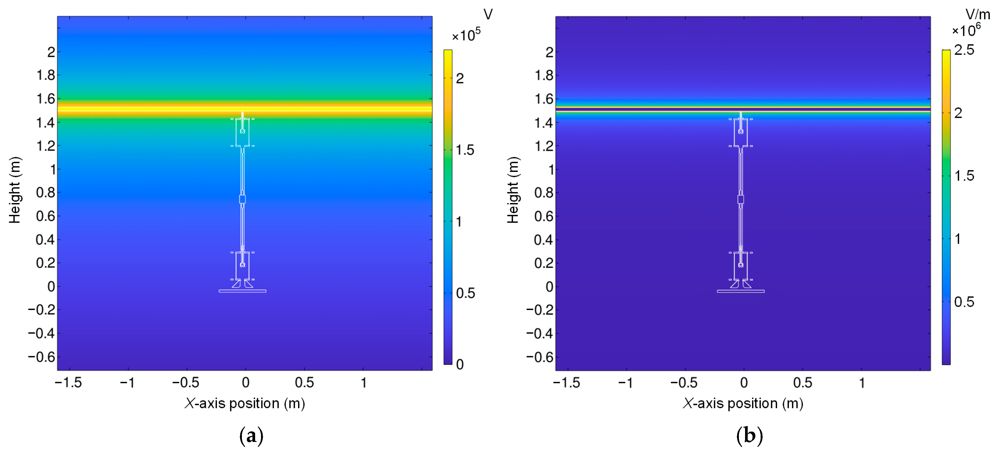
The HV contact electrode at the end-effector of the moving platform engages with a 220 kV cylindrical charged body to simulate contact with exposed cables. The electrode on the fixed platform is set to ground potential. The simulated potential and electric field intensity distributions are shown in Figure 14. Potential distribution and electric field intensity profiles were obtained by sampling surfaces of both moving and fixed platforms in the simulation model.

In this simulation, five measurement planes were selected to measure the specific distribution of the electric potential. The selected measurement positions are shown in Figure 13. The measurement results at the different positions are shown in Figure 15 and Figure 16.

The potential results in Figure 15 indicate that the potential distribution reduces nonlinearly with the distance between the mechanical arm and the cable. The potential gradient across the insulator surface exhibits smooth monotonic decay without abrupt discontinuities, indicating no localized breakdown risk. The simulation results reveal distinct potential distributions across various sampling planes. At position 1, located in close proximity to the charged conductor, the measured potentials reach a maximum of approximately 138.4 kV with a minimum of 135.2 kV, resulting in a potential differential within 3.2 kV. Similarly, position 2 exhibits potential values ranging from 79.74 kV to 80.12 kV, maintaining a variation below 0.38 kV. Position 3 demonstrates potentials between 42.50 kV and 43.70 kV, with the overall differential limited to 1.2 kV. Further measurements indicate potential variations below 4 kV at position 4 and 1.3 kV at position 5, respectively. These observations collectively demonstrate well-controlled potential distributions throughout the system. The combined analysis of potential contours and electric field strength distributions confirms that the insulator meets all insulation requirements.

For the simulation data of each cross-section, the calculation results of various mathematical characteristics are shown in

Table 4. Mathematical characteristics of simulation results.

Position Number	1	2	3	4	5
Section height (m)	1.43	1.20	0.75	0.30	0.06
Average field value (V/m)	518,838	132,756	53,853	33,074	25,811
Maximum field (V/m)	554,350	143,015	54,389	45,195	27,292
Minimum field (V/m)	217,724	51,955	45,201	31,803	11,339
Standard deviation (V/m)	75,416	20,394	1501	1735	3310

.

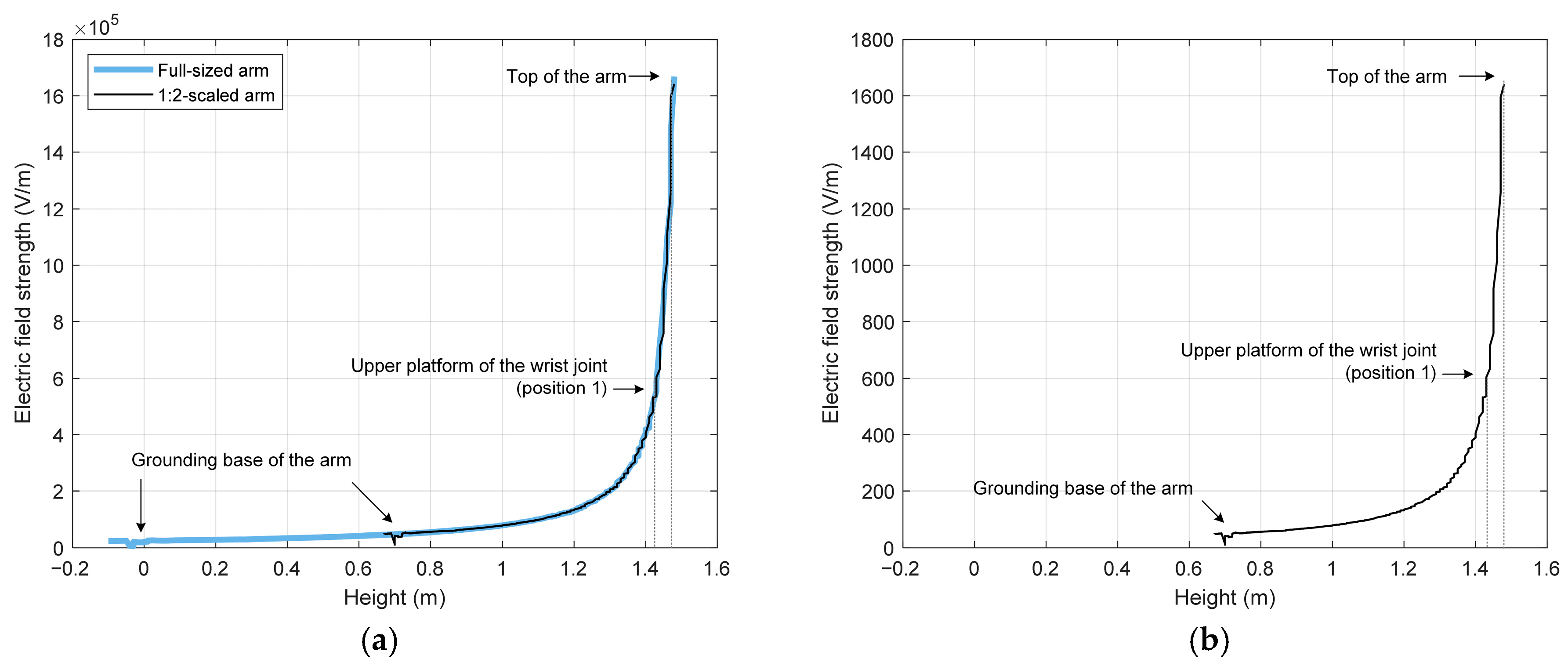
In order to prove the validity of the fitting between the simulation results and the low-voltage experimental results, we also conducted an electric field simulation of a robotic arm model with a size reduced by 0.5 times at 220 kV level, and an electric field simulation of a robotic arm model with the same size reduction at 220 V level. The results are shown in Figure 17.

From the electric field distribution curves from the bottom to the top of the original-size manipulator and the 1:2-scaled manipulator at 220 kV, it can be seen that when the size of the manipulator is reduced, the electric field distribution curves almost overlap. This is due to the self-insulating design of the mechanical arm, which has a negligible effect on the electric field. Therefore, using a 1:2-scaled manipulator does not affect the analysis of the electric field strength at the top of the manipulator. The maximum electric field strength is 1.8 × 10⁶ V/m, which is less than the air breakdown field strength.

From the electric field distribution curve of the 1:2 scaled-down manipulator from the bottom to the top at 220 V, it can be seen that compared with 220 kV, the electric field distribution curve is the same, and the electric field strength is 1/1000 times that at 220 kV. Therefore, the electric field result measured using 220 V voltage can be multiplied by the scaling factor to obtain the actual electric field strength at the top of the original-size manipulator at 220 kV.

Figure 16 demonstrates that the electric field intensity is predominantly concentrated within a limited region of less than 0.05 m surrounding the charged cable. Longitudinal analysis reveals that both the mechanical arm structure and its surrounding environment maintain electric field intensities below 80 kV/m. Laterally, potential distributions across all five sampling planes exhibit smooth profiles without distortion. Given the dielectric strength thresholds of 300 kV/m for air and 2000–3000 kV/mm for typical polyester and rubber materials (according to IEC 60243), none of the insulating components in the system are susceptible to breakdown under the operational voltage conditions of cable tunnels. Due to the insulation performance of the mechanical arm, the extra insulation layer of conventional live-line operation mechanical is negligible, and the insulating materials for the joints and the arm are lighter than the metallic material of traditional mechanic arms. The total quality of the proposed mechanical arm is 4.7 kg. This amount of the arm’s mass allows the mechanical arm to cover large inspection space because the movement of arm is not likely to cause significant gravity center displacement of the carrier. Therefore, the self-insulating joint mechanism of the mechanical arm has been appropriately designed to meet the dielectric and inspection requirements, ensuring reliable performance in the specified working environment.

6. Experiment

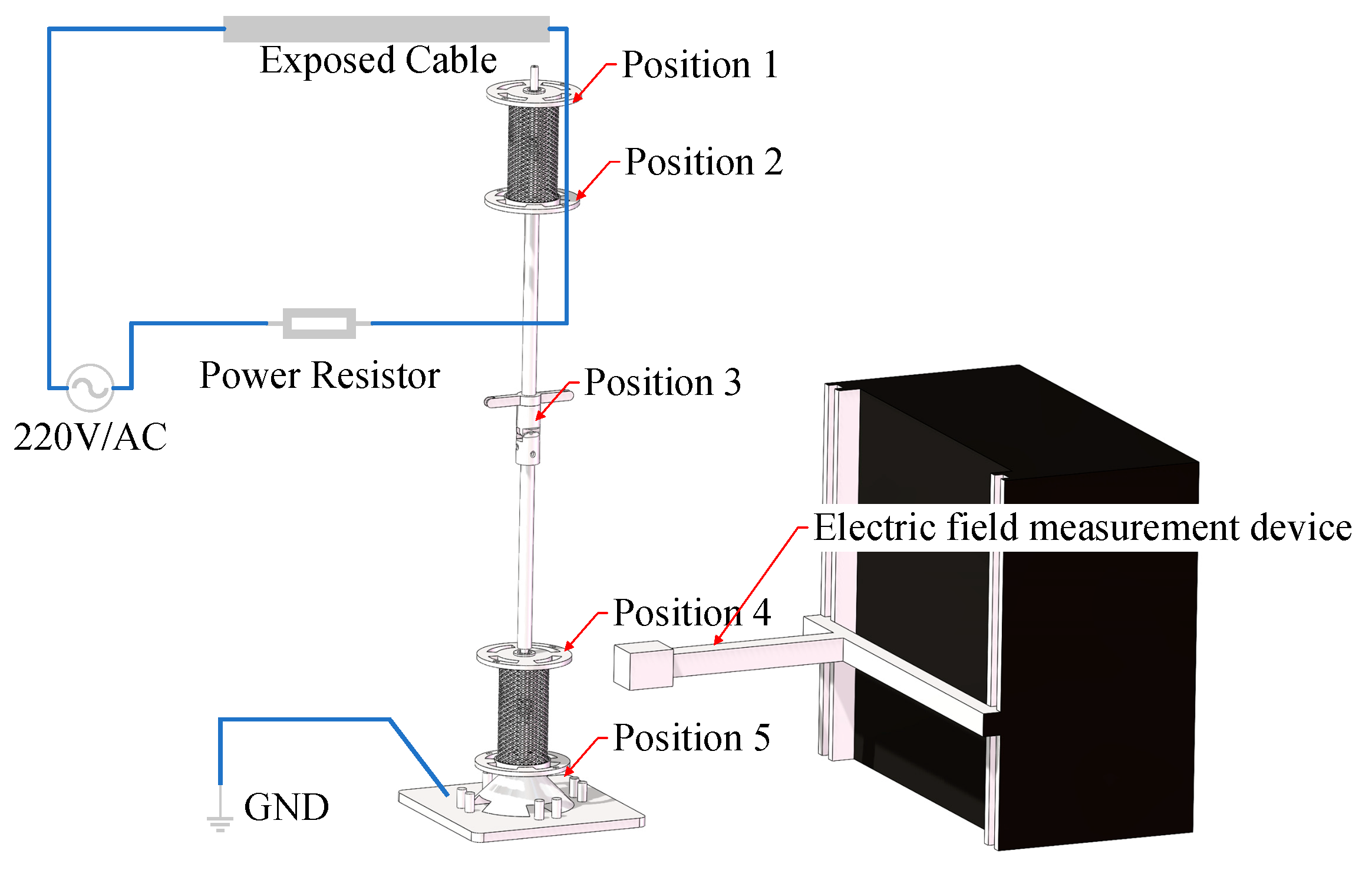
Since the electric field measurement device is not allowed to approach the HV live-operating power cable, we made a proportionally reduced physical model of the mechanical arm to verify the reliability of the simulation results in practical applications. The physical model’s length, width, and height are at 1 to 2 scale ratio of the designed mechanical arm, respectively. Therefore, the experiment uses a 220 V voltage level, and the electric field data is collected at the corresponding position of the self-insulating mechanical arm experimental model through an electric field measuring instrument to verify the consistency between the actual results and the simulation. The five measurement positions in Figure 18 are selected according to the simulation model in Figure 13.

This scheme provides an effective approach for low-voltage experimental verification of the insulation performance of high-voltage equipment.

The following are the experimental details. The experimental flow chart is shown in Figure 19a. The experimental site picture is shown in Figure 19b. During the experiment, the indoor temperature was maintained at 25 degrees Celsius, and the air humidity was 40%. The positioning accuracy of the electric field measuring instrument was ±0.05 mm.

The electric field measurement results are shown in

Table 5. Electric field measurement experiment data collection results.

Position Number	1	2	3	4	5
Measured Electric Field V/m	377	121	52	10	3

.

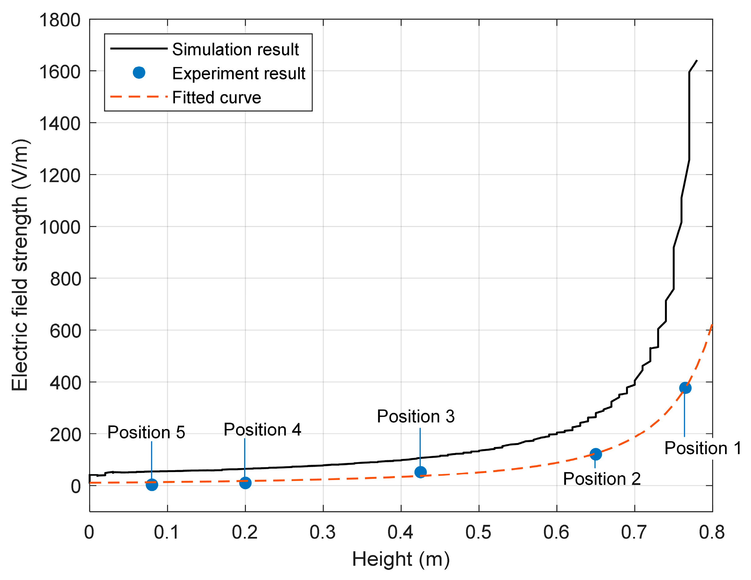
The calculated electric field distribution along the mechanical arm is shown as the solid line in Figure 15. The measured electric field distribution at positions 1–5 is shown as the dots and the fitted curved based on the measured results is drawn to compare to the calculated results.

Figure 20 shows that both the simulation and experiment results have a decreasing tendency along the mechanical arm, indicating that the proposed self-insulating mechanical arm has reliable insulation characteristics in a concealed space working environment. The simulation result is 27.2% larger than the experiment result because the probe of the electric field measurement device is made of stainless steel. The probe itself could interfere with the accuracy of field measurement and cause a decreased offset. However, the electric field tendencies of simulation and experiment results are consistent.

7. Summary and Outlook

This manuscript presents the design of a self-insulating mechanical arm for live-line maintenance operations in confined cable tunnel environments. The mechanical arm features a novel self-insulating joint mechanism consisting of an internal universal joint support structure and an external flexible dielectric body, actuated by four insulated tension cables. The workspace is an oblate ellipsoid with minor and major axes measuring 1.25 m and 1.65 m, respectively, covering the concealed space in the cable tunnel, while the arm’s quality is 4.7 kg. This innovative design physically separates the drive system from the mechanical arm’s working components, offering significant advantages over conventional live-line mechanical arms.

The maximum electric field intensity along the mechanical arm is 74.3 kV/m, significantly less than the air breakdown field threshold when the arm approaches the live-operating 220 kV power cable. The potential and electric field distributions demonstrates the compliance with self-insulation performance requirements. The self-insulating design significantly enhances insulation performance and reduces the arm mass in 220 kV power cable tunnel environments.

While demonstrating these advancements, the current design shows certain limitations including relatively low torque utilization efficiency in the drive system and insufficient vibration resistance at the end-effector when subjected to disturbances. Future research will focus on improving these aspects through optimized drive mechanisms and enhanced vibration damping solutions.