Experimental Test of Continuous Wave Frequency Diverse Array Doppler Radar ^†

Abstract

The frequency diverse array (FDA) is an antenna array architecture capable of beamforming in both range and angle. It improves upon the traditional phased array (PA), which can only achieve beamforming in angle. The FDA is configured to simultaneously scan in both range and angle using small frequency offsets across radiating elements, allowing beam scanning to occur from low-complexity RF hardware configurations. This work documents experimental data collections from four system evolutions of a prototype linear continuous wave (CW) FDA radar system, with emphasis on validating the system behavior at the signal model level. Data collected from these testing evolutions showcase the system as a potential low-complexity perimeter surveillance system with an auto-scanning mainbeam feature.

1. Introduction

The frequency diverse array (FDA) was first introduced in a series of works by Antonik and collaborators [1,2,3]. In such an array, linearly progressive frequency offsets were applied between uniformly spaced elements, generating range–angle coupled beampatterns with periodic modulations in range, angle, and time [4,5]. The resulting auto-scanning behavior is accomplished without the use of any other electronics or external phase-shifting hardware. Multi-mission, multi-mode applications have also been proposed in [1,2,3], including simultaneous synthetic aperture and moving target indication.

The frequency diversity of the array introduces range–angle beamforming, which improves upon the angle-only beamforming from a phased array (PA) radiating a single carrier frequency. By decoupling the range and angle dimensions, steerable localizations in energy can be created in the far-field pattern. Work in this area includes the random FDA [6], FDA sub-array architectures [7,8,9], non-linear frequency offsets [10,11,12,13,14,15], algorithmic optimizations of the FDA beampattern [16,17], multiple input multiple output (MIMO) [18], false target generation [19], electronic counter-counter measures (ECCM) [20], and FDA wireless power transfer architectures [21,22,23], among others.

Although much theoretical work has been conducted in the area of FDAs, only a limited number of array builds have been reported in the open academic literature. The current list of builds known to the authors includes the following:

• Antonik [24]: $3\times 5$ planar array with a $3\times 1$ sub-array structure with 5 distinct frequencies. The transmit array had a designed carrier frequency of 3 GHz, and [24] features several narrowband far-field collections. The signal generation was accomplished by signal generators.
• Brady [25]: two element FDA waveform testbed with a (typical) carrier frequency of 10 GHz. Signal generation was accomplished by an arbitrary waveform generator (AWG).
• Eker [26]: $1\times 10$ linear frequency modulated (LFM) FDA. Carrier frequency of 3 GHz with signal generation accomplished by a single LFM-CW source and a delay network.
• Çetintepe [27]: re-built and improved the $1\times 10$ LFM FDA in [26]. The build had a carrier frequency of 3 GHz and used a single LFM-continuous wave (CW) source and a delay network to generate the transmit signals.
• McCormick and Kellerman [28,29]: MISO LFM FDA with a $1\times 8$ transmit array. The transmit array had a designed carrier frequency of 3.3 GHz and used an RFSoC as the transceiver.
• Munson [30]: $1\times 3$ linear FDA using Ettus Universal Software Radio Peripheral (USRP) x310 software defined radios (SDR) as the transceivers. The array had a designed carrier frequency of 2.4 GHz.
• Munson [31]: $1\times 2$ linear FDA with binary phase-shift keying modulations using an AWG. The array had a designed carrier frequency of 720 MHz.

There also exists one hardware implementation by Huang [32,33] but with no array build.

The initial setup, we show the results of the first experimental FDA data collections using SDR platforms, which have recently seen increasing use in the academic literature (AOA/DOA [34,35,36,37,38], phased arrays [39], communications systems [40,41,42,43], and FMCW radars [44]). These collections are designed to demonstrate the FDA as a low-complexity perimeter surveillance system with an auto-scanning mainbeam feature, with an emphasis placed on validating the signal model-level behavior of the system. The collections feature moving targets, including cars and drones, commonly found in perimeter surveillance applications. We document the system evolution from initial far-field pattern measurements to time–frequency analysis of micro-Doppler features generated by a rotating blade. Using linear CW FDA radar, the following are our contributions to FDA research:

• We experimentally demonstrate both the temporal periodicity and angular scanning behavior of the FDA far-field pattern.
• We experimentally demonstrate basic radar functionality inside an anechoic chamber with a binary target detection test.
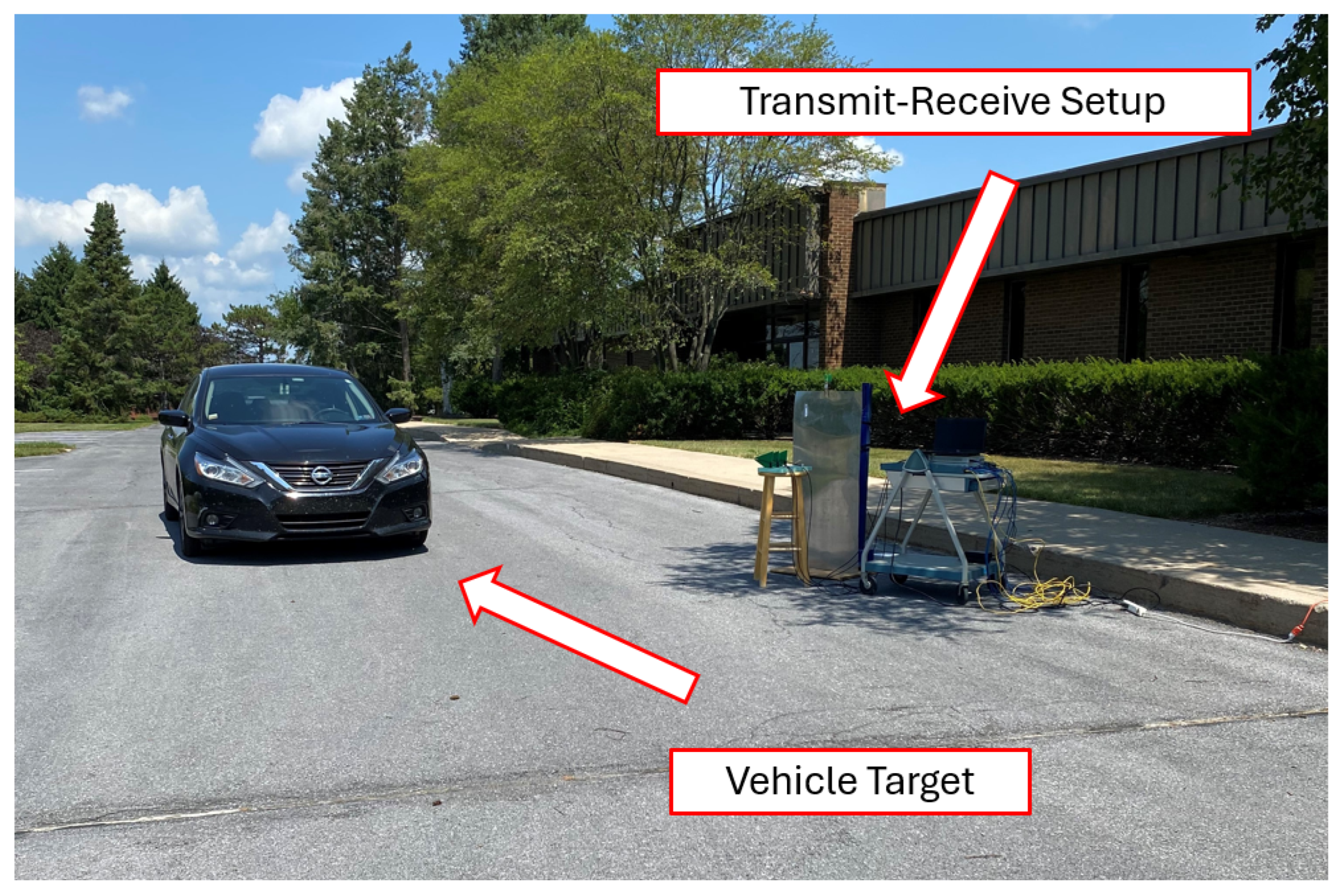
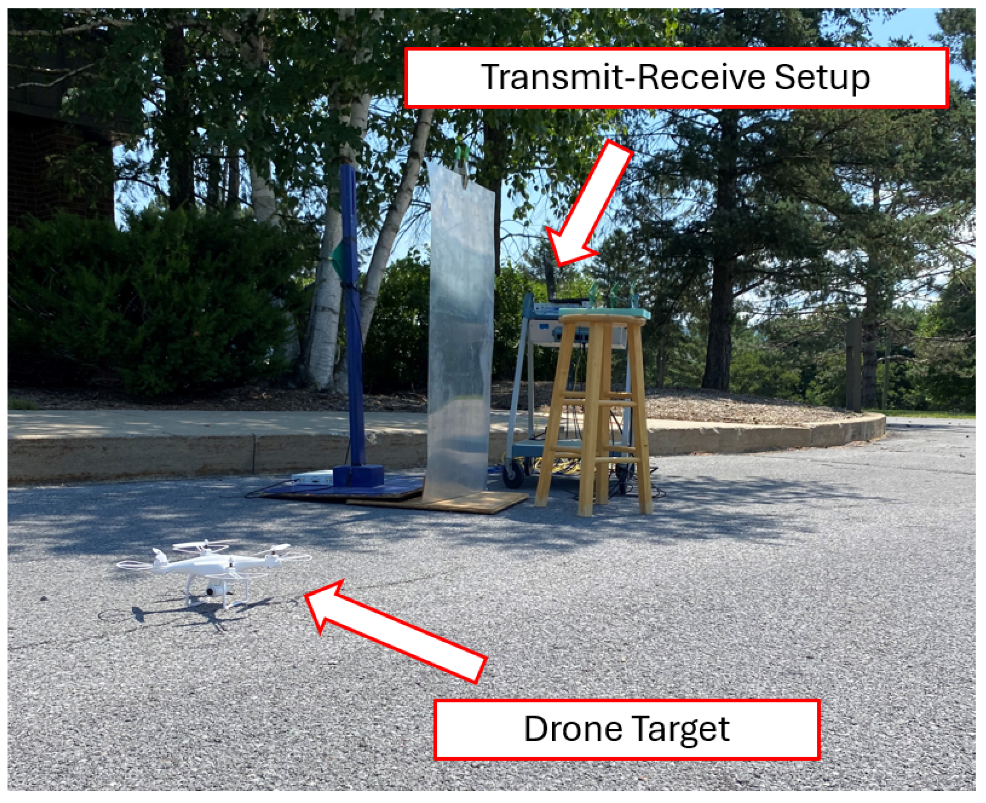
• We capture the Doppler information from two different moving targets: a car and a drone.
• We use time–frequency analysis on experimentally captured micro-Doppler data to extract information about rotating propellers.

The initial setup and testing of the system are described in our previous work in [30]. The description and numbering of the data collections in this paper are given in

Table 1. Labeling and descriptions of data collections in this paper.

Label	Description
Collection I	Far-field Beampattern
Collection II	Stationary Target Reflection
Collection III	Moving Target Reflection
Collection IV	micro-Doppler Signature

. The remainder of the paper is organized as follows. Section 2 shows the results of the far field data collection. Section 3 shows the results from stationary target testing inside an anechoic chamber. Section 4 shows the results and detections of moving targets in a radar scene, and Section 5 shows the time–frequency analysis of an experimentally collected micro-Doppler generated by a rotating blade.

2. Data Collection I: Far-Field Beampattern

In this section, two key features of the FDA beampattern, namely, temporal periodicity at a fixed location and angular mainbeam auto-scanning with increasing fast-time, are experimentally demonstrated and shown to closely follow the theoretical and experimental results in [24]. The experimental setup for this data collection is shown in Figure 1, and a photograph of the general system setup is shown in Figure 2.

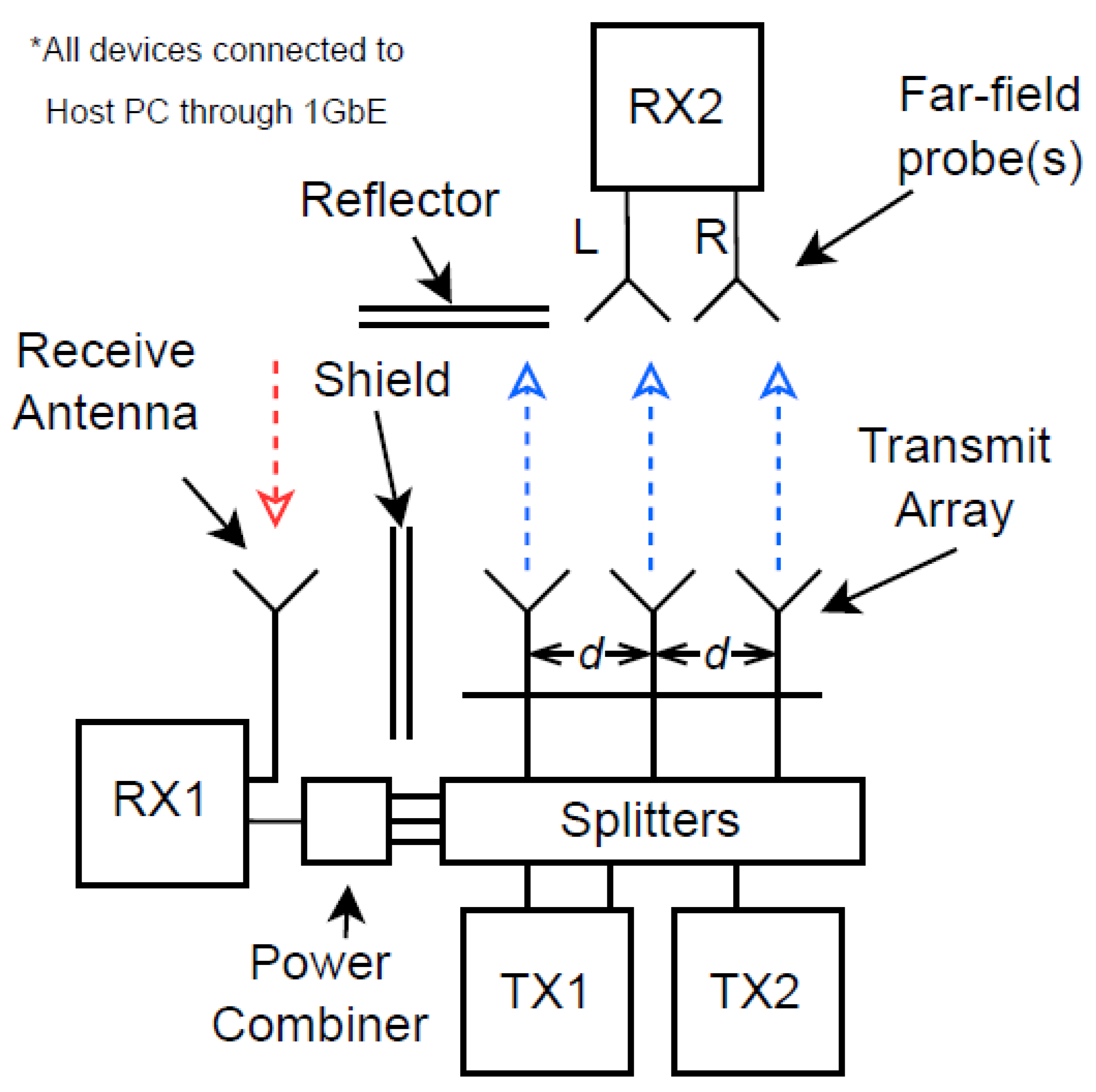
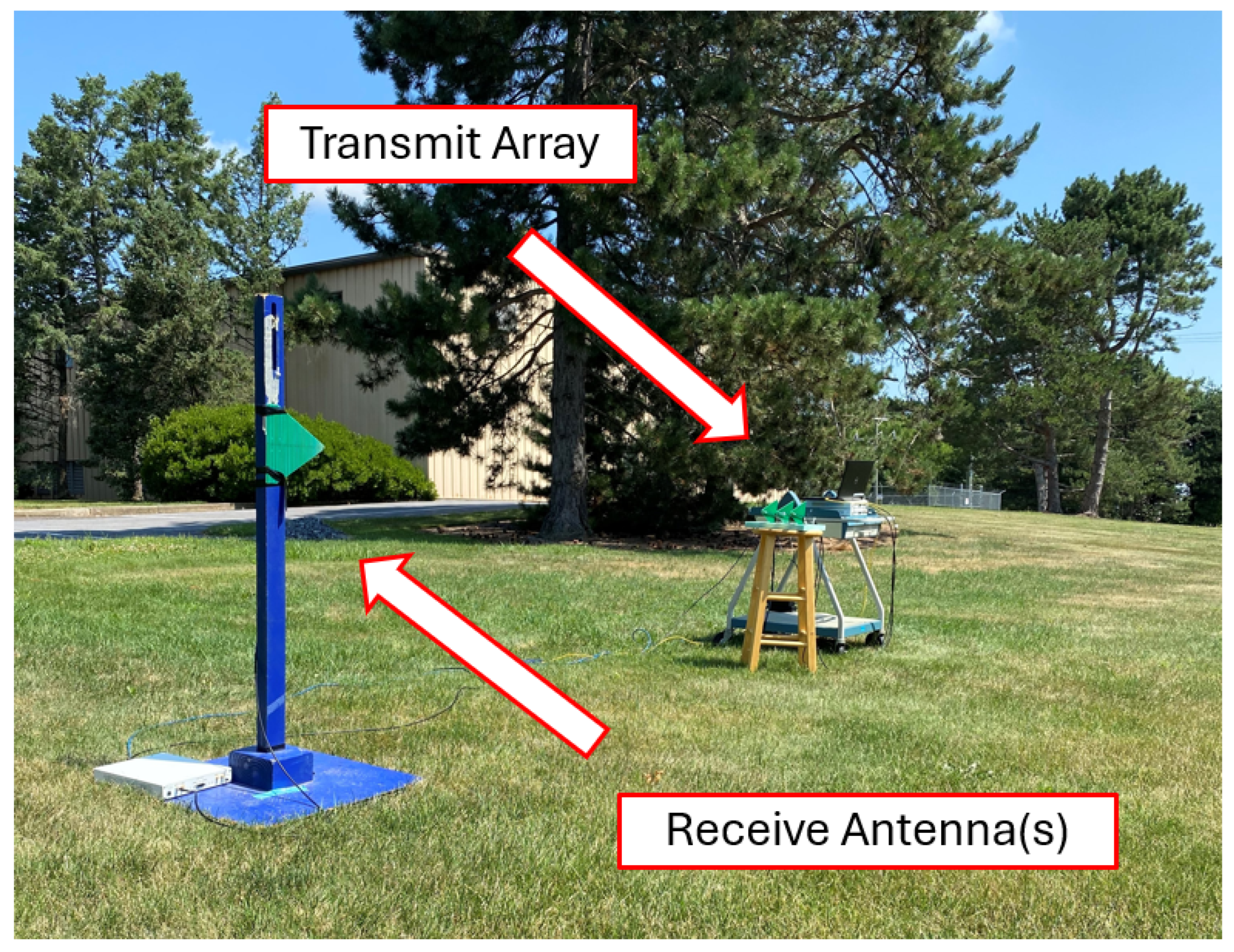
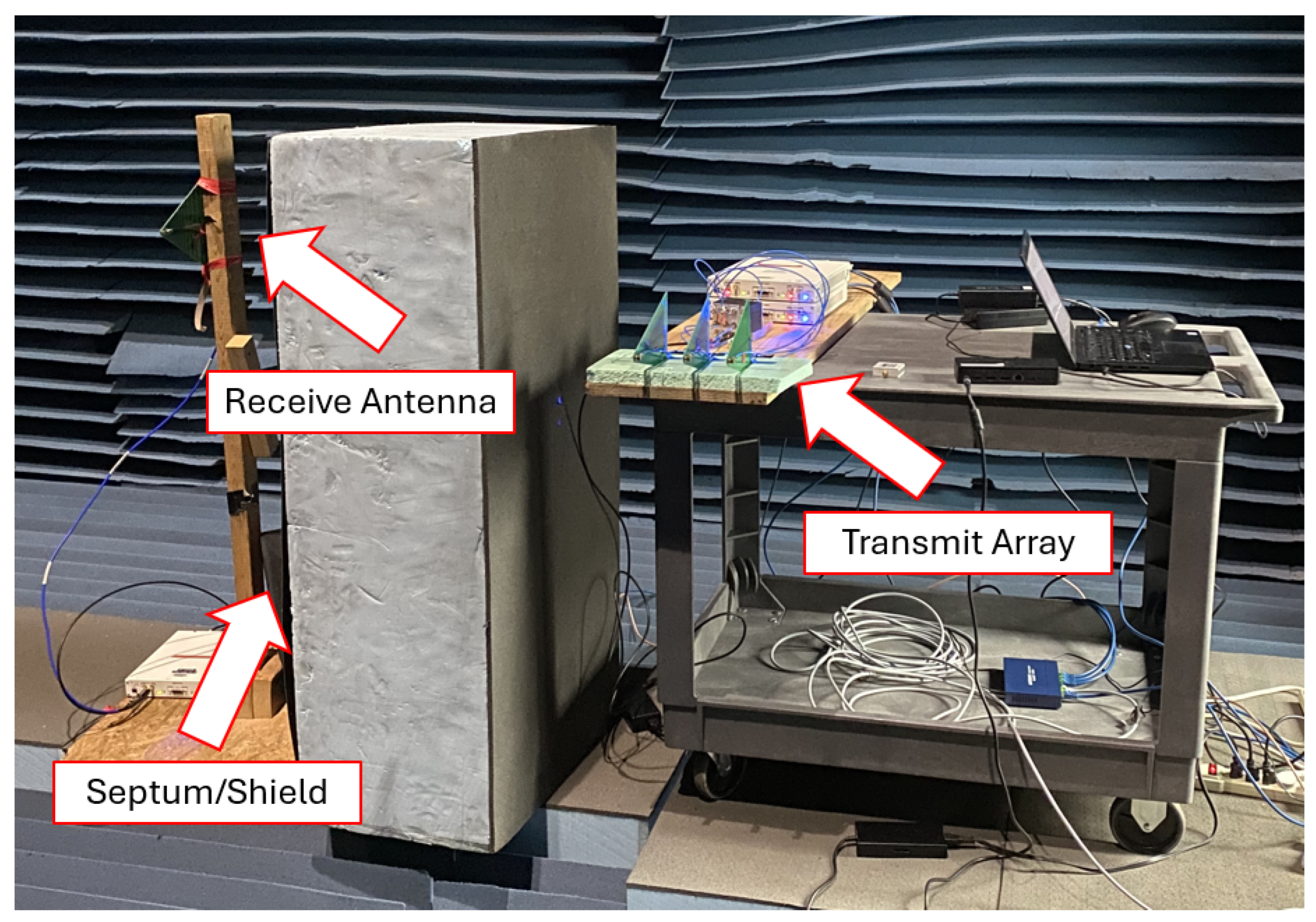
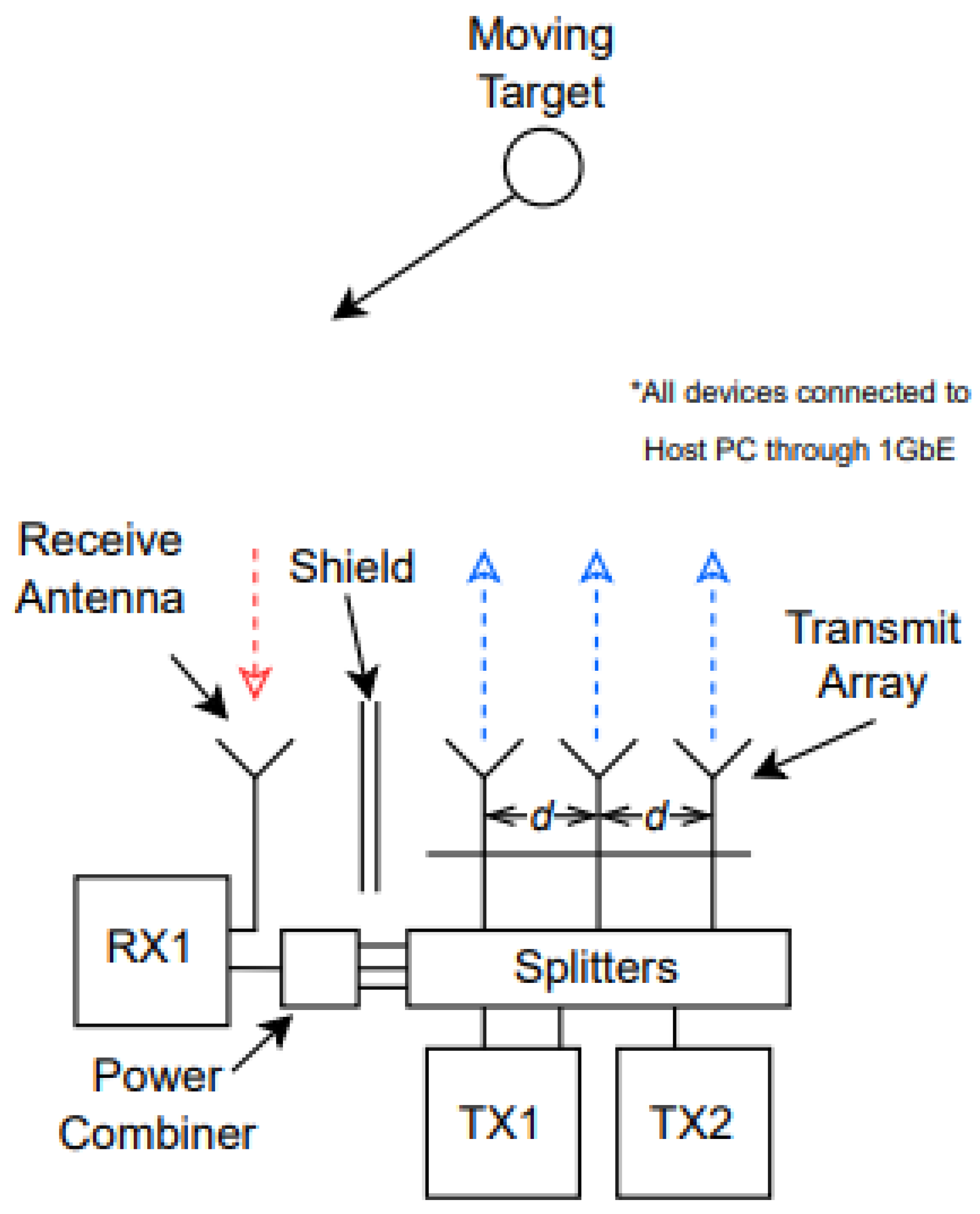
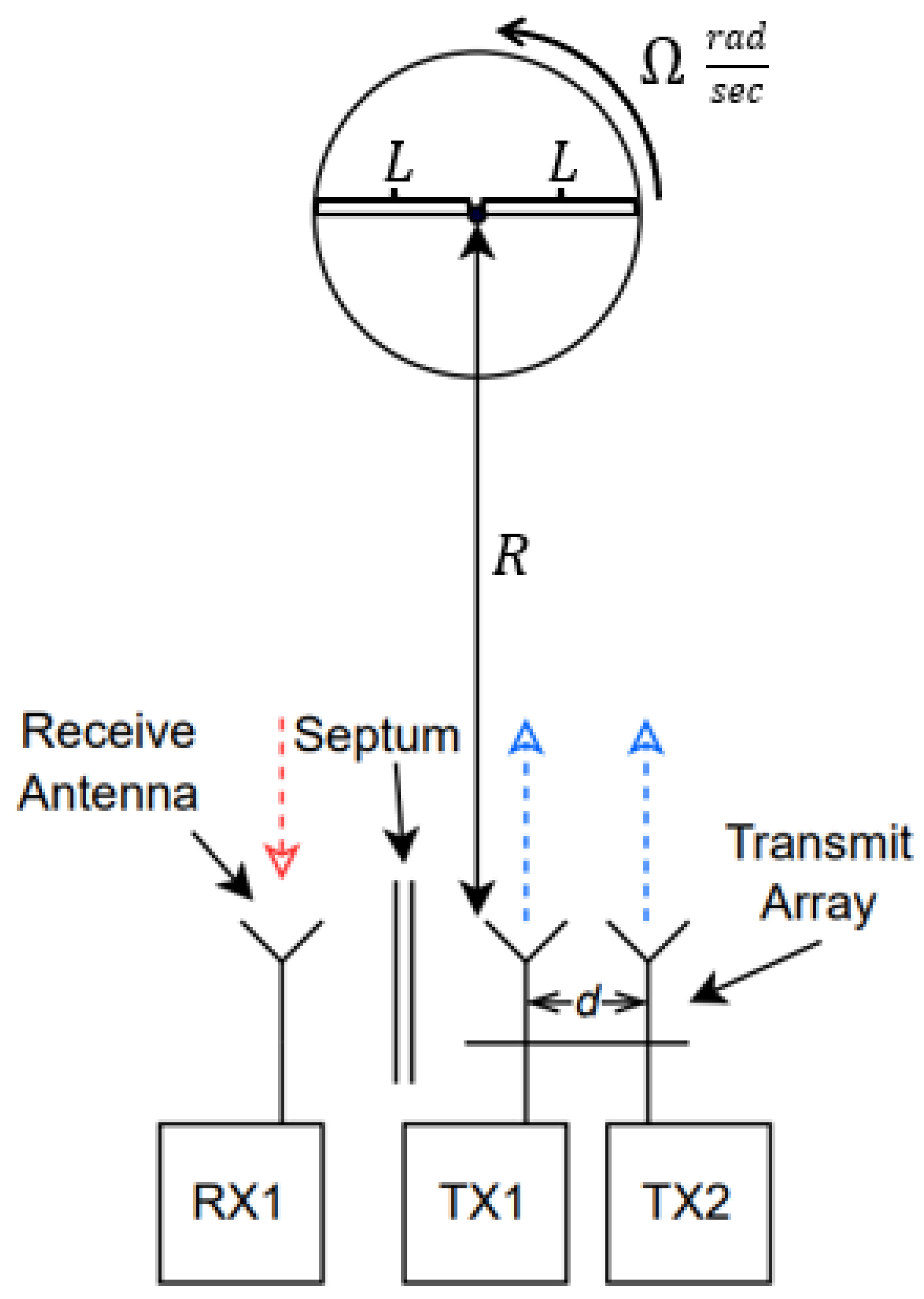
2.1. Hardware and System Overview

The antennas and components with respect to collection are given in

Table 2. RF component list for the transmit (Tx) antennas, receive (Rx) antennas, power splitters, and power combiners.

Component	Manufacturer/Part #	Collection
Log-Periodic Tx Antenna	WASVJB 0.85–6.5 GHz	I, II, III
Log-Periodic Rx Antenna	Walfront 0.6–6.0 GHz	I, II, III
Log-Periodic Tx Antenna	WASVJB 2.1–11 GHz	IV
Log-Periodic Rx Antenna	WASVJB 2.1–11 GHz	IV
2-way Power Splitter	Minicircuits ZAPD-30-S+	I, II, III
4-way Power Combiner	Minicircuits ZN4PD1-50-S+	I, II, III

. The connectors for each collection are SMA type, and common path-length cabling is used on the transmit paths. Each greenUSRP X310 houses a motherboard that supports two additional daughterboards, which can perform both analog-to-digital and digital-to-analog conversions. Each UBX-160 daughterboard is capable of producing one transmit signal; thus, the block diagram in Figure 1 shows a physical setup where three signals are produced from two X310 SDRs. The TwinRX daughterboard is used as the receive hardware in Data Collections I, II, III, and IV. The UBX-160 is transmit hardware for Data Collections I, II, and III. Data streaming limitations on the host PC require two signal generators as the transmit system for collection IV. The data is offloaded from the X310 SDR(s) to the host PC for display via a datastream. The Python (version 3.9.9) API (enabled during the CMake stage when building the source code) is used to configure both the devices and the metadata for the datastream.

2.2. Far-Field Signal Model

Our signal model follows Correll and Rigling in [10,11], where the theoretical FDA far-field pattern at a point having radius R and angle $\theta$ at fast-time t is the coherent summation

$$F(t;R,\theta )=\sum _{n=0}^{N-1}{e}^{j2\pi f_n(t-R_n/c)}.$$

(1)

Here, $f_n=f_0+n\Delta f$, where $f_n$ is the transmit frequency at the nth element of a linear FDA having carrier frequency $f_0$, frequency offset parameter $\Delta f$, N total elements, and element indexing $n=0,1,...,N-1$. $R_n=R-ndsin\theta$, where $R_n$ is the distance from the nth transmit element to the far-field point $(R,\theta )$ for an array with inter-element spacing $d={\lambda }_0/2$.

Note that Equation (1) is used to track the coherent combination of the far-field pattern at a given point $(R,\theta )$ and does not contain a scalar to model the fall-off of incident power. Additionally, this idealized model assumes isotropic radiation and no mutual coupling, no amplitude variation, no phase noise, and no unknown frequency offsets or element location inaccuracies.

2.3. Far-Field Distance Calculation

In [45], the problem of evaluating the Fraunhofer zone (FZ) for FDA with equal inter-element spacing is studied. The relative frequency band $\delta f=(f_{max}-f_{min})/(f_{max}+f_{min})$ and overlap factor ${\xi }_{ov}=\Delta f/\Delta S_{part}$ are defined and help characterize FZ error for FDA with $f_n=f_0+n\Delta f$. $\delta f$ characterizes the bandwidth of the array with respect to the array center frequency, and ${\xi }_{ov}$ characterizes the spectral overlap between array elements with respect to the partial signal spectrum $\Delta S_{part}$ and inter-element frequency offset $\Delta f$.

In this work, the bandwidth of each collection is small relative to the carrier frequency of the array, yielding $\delta f\ll 1$. Additionally, since each array element radiates a constant tone, $\Delta S_{part}\to 0$, yielding ${\xi }_{ov}\gg 1$. Thus, we make the monochromatic assumption when calculating the range to the farfield $R_{ff}$. Following [45,46], this range is

$$R_{ff}\ge {\displaystyle \frac{2D^2}{{\lambda }_0}}={\displaystyle \frac{2{\left((N-1)\frac{{\lambda }_0}{2}\right)}^2}{{\lambda }_0}}={\displaystyle \frac{1}{2}}{\lambda }_0{(N-1)}^2.$$

(2)

The far-field distance for each collection is calculated using Equation (2) and summarized in

Table 3. Far-field distance of each collection calculated using Equation (2).

Collection	${\mathit{f}}_0\left(\mathbf{GHz}\right)$	N	${\mathit{R}}_{\mathit{ff}}\left(\mathbf{m}\right)$
I	2	3	0.2998
II	2	3	0.2998
III	2	3	0.2998
IV	5.9	2	0.0254

.

2.4. Expected Behavior at Baseband

We expect the same far-field magnitude behavior seen at RF to also exist at baseband. To show this, we begin by rearranging Equation (1) as follows

$$\left|F(t;R,\theta )\right|=\left|e^{j2\pi f_{0}t}\sum _{n=0}^{N-1}{e}^{j2\pi \Delta f(t-R_n/c)}\right|.$$

(3)

The magnitude of Equation (3) can be simplified using $|z_1{z}_2|=|z_1\left|\right|z_2|$ (where $z_1,z_2$ are complex numbers), resulting in the simplified expression

$$\begin{array}{cc}\hfill |F_{RF}(t;R,\theta )|& =\left|e^{j2\pi f_{0}t}\right|\left|\sum _{n=0}^{N-1}{e}^{j2\pi \Delta f(t-R_n/c)}\right|\hfill \\ \hfill & =\left|\sum _{n=0}^{N-1}{e}^{j2\pi \Delta f(t-R_n/c)}\right|.\hfill \end{array}$$

(4)

The magnitude of the baseband signal when down converted at the carrier frequency $f_0$ is

$$\begin{array}{cc}\hfill |F_{bb}(t;R,\theta )|& =|e^{j2\pi f_{0}t}\left[\sum _{n=0}^{N-1}{e}^{j2\pi \Delta f(t-R_n/c)}\right]·e^{-j2\pi f_{0}t}|\hfill \\ \hfill & =\left|\sum _{n=0}^{N-1}{e}^{j2\pi \Delta f(t-R_n/c)}\right|.\hfill \end{array}$$

(5)

Thus, it can be seen through comparison of Equations (4) and (5) that $|F_{RF}(t;R,\theta )|=|F_{bb}(t;R,\theta )|$.

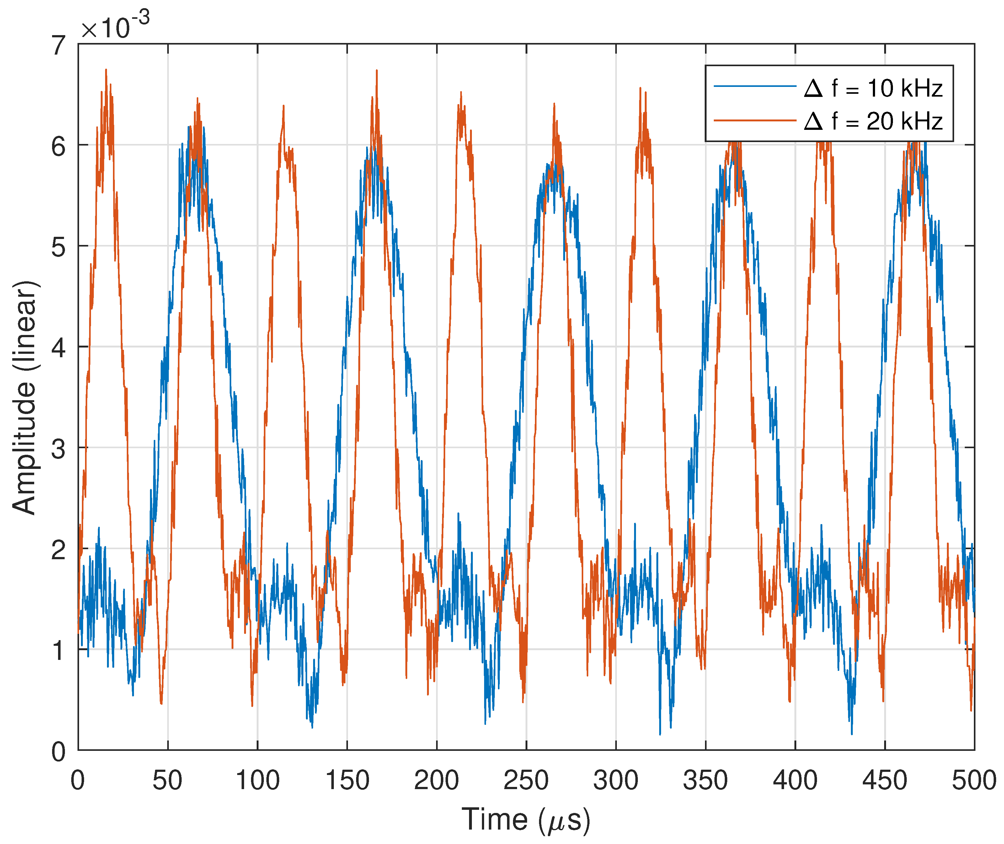
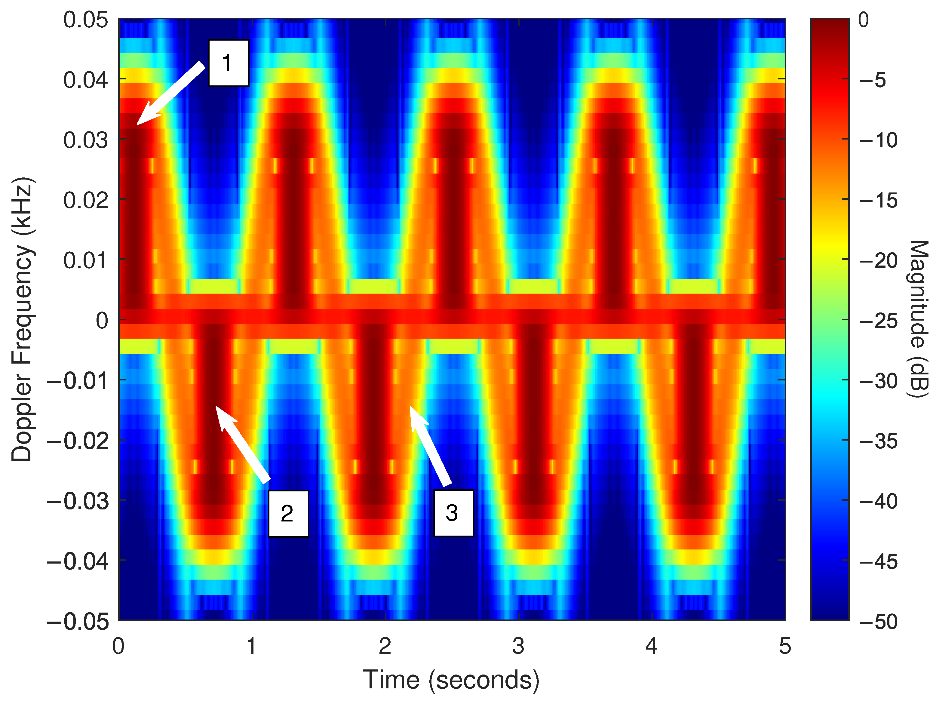
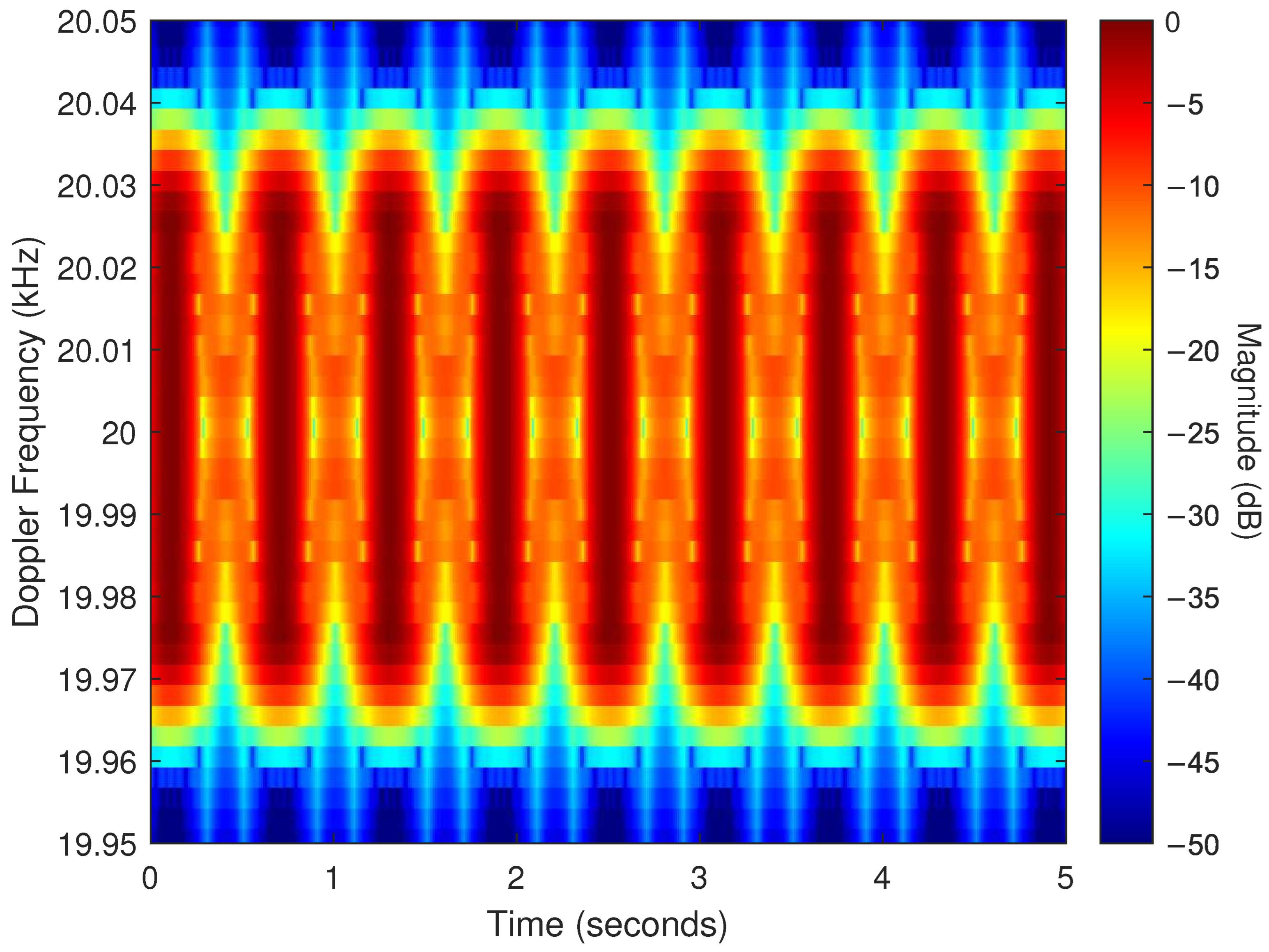
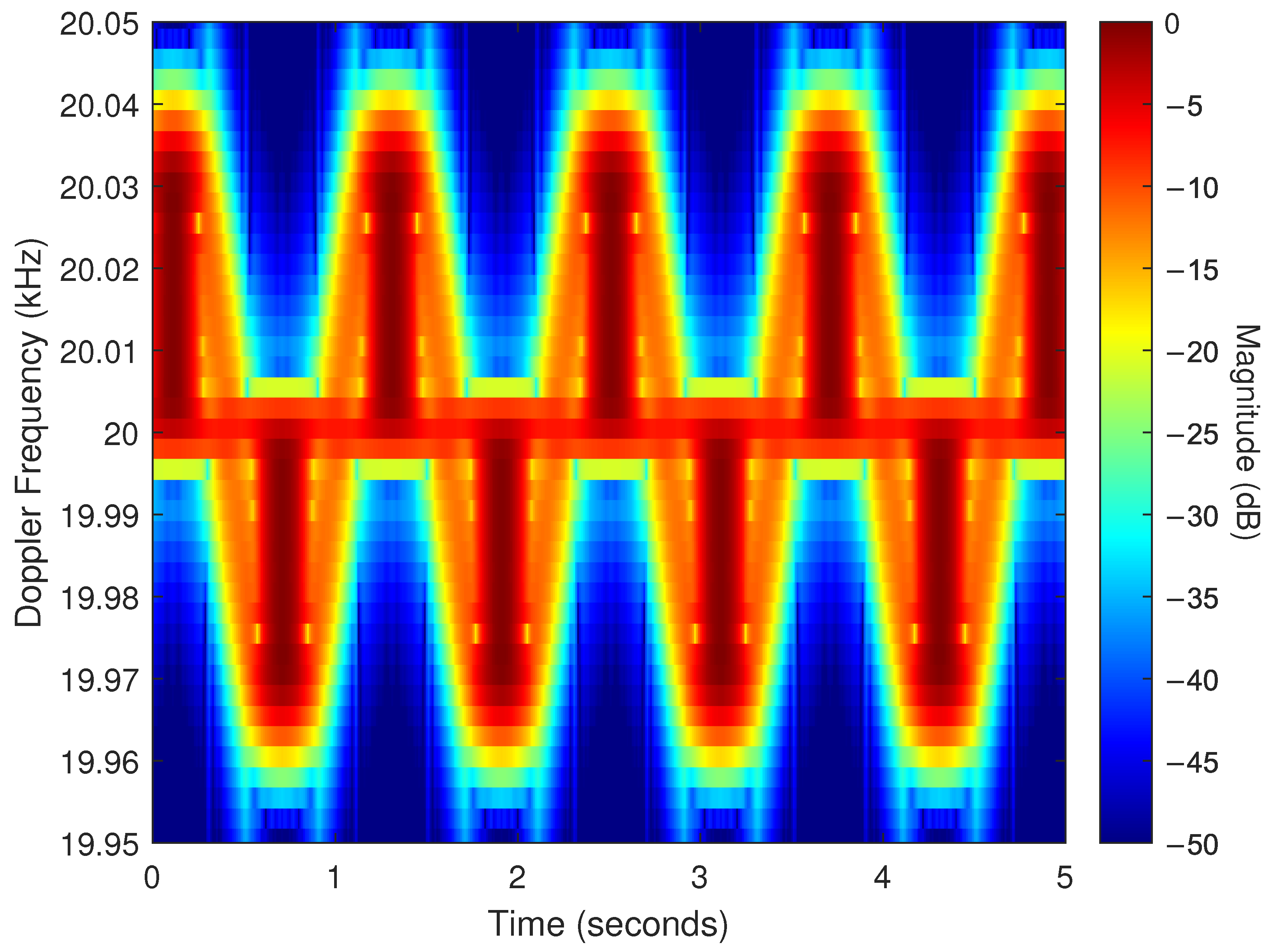
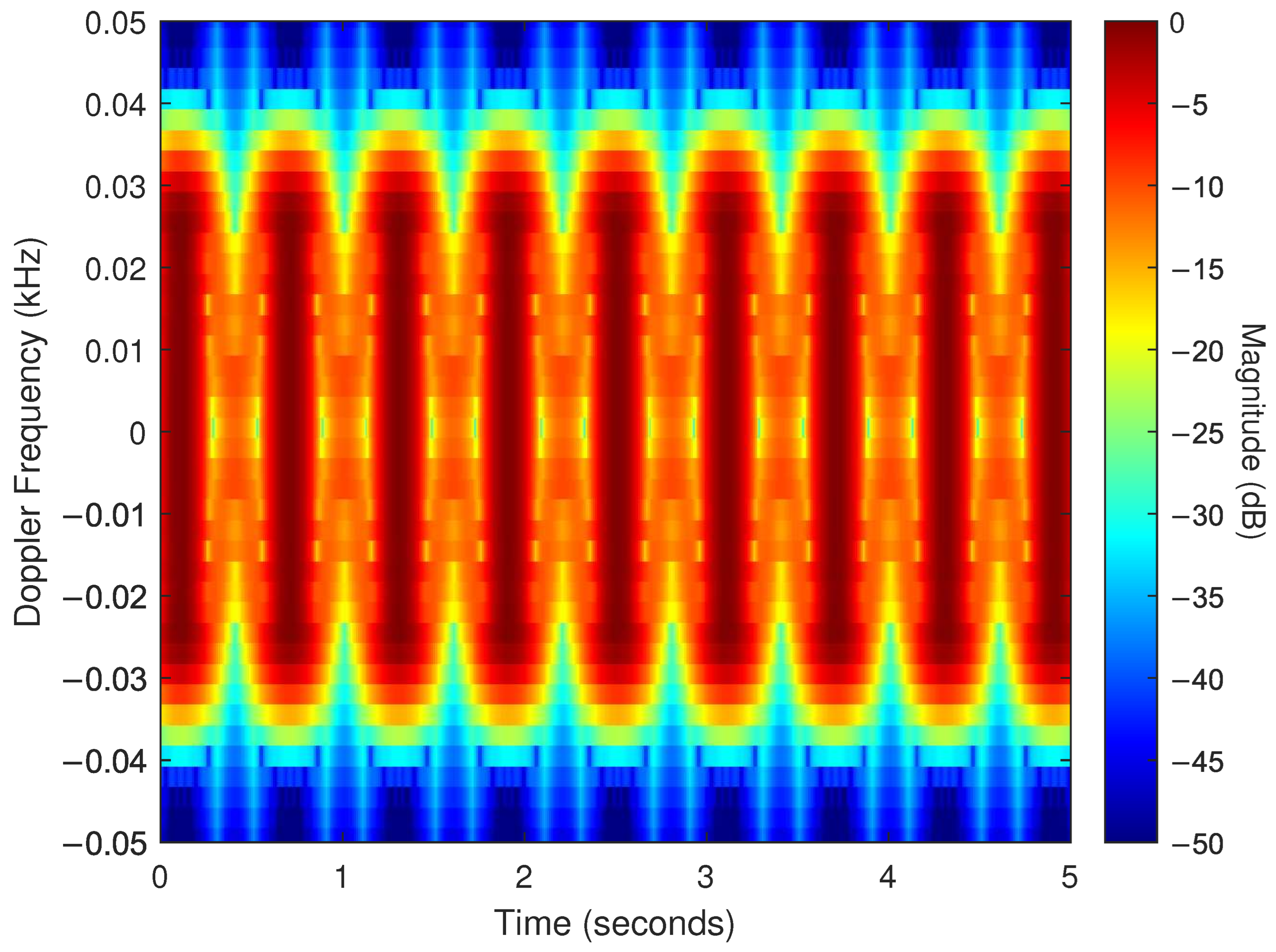
2.5. Temporal Periodicity of the Far-Field Pattern

2.5.1. RF Hardware Collection

For a fixed collection location $(R,\theta )=(R_o,{\theta }_o)$ and an FDA transmitting a linearly progressive frequency offset $\Delta f$, Antonik [24] showed that the expected periodicity in time of the far-field pattern is $1/\Delta f$. This result is also seen in [4,5]. To demonstrate that this behavior continues at baseband in our system setup, a bench test was conducted using three signals fed into a power combiner whose output was then sampled by an X310 SDR. The frequency spacing between the signals followed a linear frequency offset scheme to mimic the coherent summation of the FDA beampattern in the far field. The temporal periodicity results for frequency offsets of 10 kHz, 12 kHz, 20 kHz, 50 kHz, 100 kHz, 250 kHz, and 500 kHz were recorded and averaged over 100 peaks at each frequency offset. These results are shown in

Table 4. Hardware bench test of temporal magnitude periodicity.

$\Delta \mathit{f}$ (kHz)	Measured ($\mathsf{\mu }\mathbf{s}$)	Theoretical ($\mathsf{\mu }\mathbf{s}$)
10	99.33	100.00
12	83.62	83.33
20	49.89	50.00
50	20.04	20.00
100	9.95	10.00
250	4.04	4.00
500	2.00	2.00

.

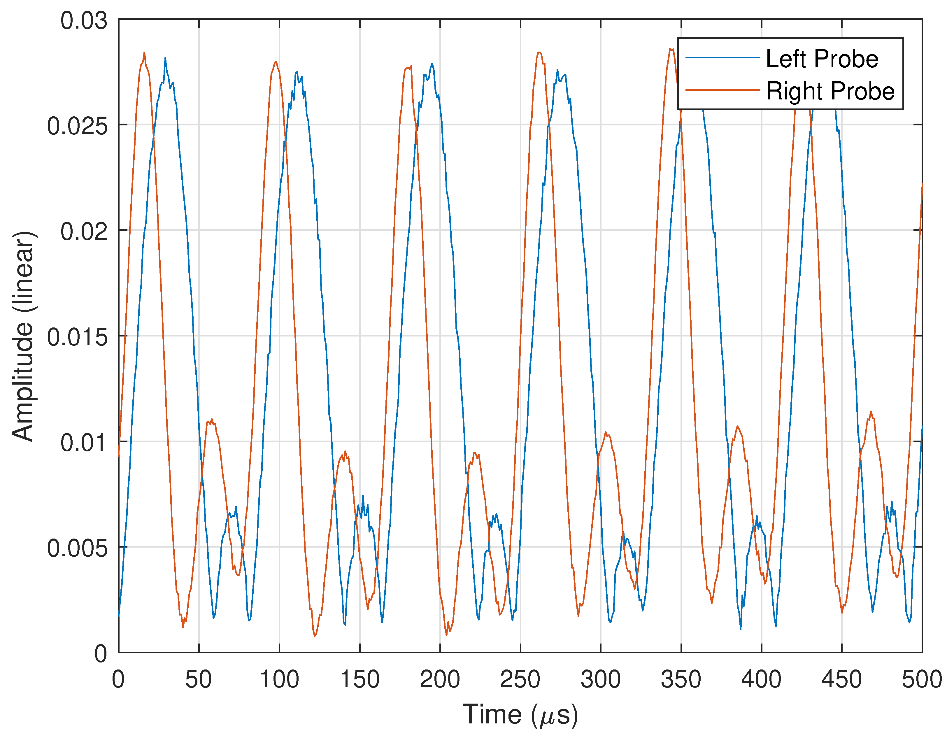
2.5.2. Far-Field Probe Collection

Figure 3 shows the far-field measurements at a fixed location $(R_0,{\theta }_0)=(4.57\mathrm{m},0\text{°})$ for linearly progressive frequency offset pairs $\Delta f=10\mathrm{kHz}\mathrm{and}20\mathrm{kHz}$, respectively. In Figure 3, it can be seen that doubling/halving the frequency offset between elements results in a halving/doubling of the period, with measured temporal periodicities $T_p=1/\Delta f=99.28\mathsf{\mu }s$ $\mathrm{and}50.50\mathsf{\mu }s$ when $\Delta f=10\mathrm{kHz}\mathrm{and}20\mathrm{kHz}$, respectively.

2.6. Angular Scan with Time

The expression for the time to scan through an angular range is [24]

$$\Delta t={\displaystyle \frac{(d/{\lambda }_0)}{\Delta f}}(sin{\theta }_1-sin{\theta }_2),$$

(6)

where ${\theta }_1$ and ${\theta }_2$ are the angles through which the scan takes place. Figure 4 shows the results of a scan over ${\theta }_1=-10$°, ${\theta }_2=10$°. The expected scan time for this angular spacing with $\Delta f=12$ kHz is $|\Delta t|=14.47\mathsf{\mu }\mathrm{s}$. The measured average angular scan time of $15.20\mathsf{\mu }\mathrm{s}$ falls within the measured values in [24].

Figure 1. General block diagram of the FDA radar setup used in Collection I and Collection II with arrows indicating direction of wave propagation, where blue arrows indicate propagation from the transmit antenna and red arrows indicate propagation towards the receive antenna. Note the left (L) and right (R) probe labels corresponding to the collection shown in Figure 4.

Figure 1. General block diagram of the FDA radar setup used in Collection I and Collection II with arrows indicating direction of wave propagation, where blue arrows indicate propagation from the transmit antenna and red arrows indicate propagation towards the receive antenna. Note the left (L) and right (R) probe labels corresponding to the collection shown in Figure 4.

Figure 2. Photograph of the general setup for Data Collection I.

Figure 2. Photograph of the general setup for Data Collection I.

Figure 3. Overlayed probe captures at $(R_0,{\theta }_0)=(4.57\mathrm{m},0\text{°})$ showing temporal periodicity generated by an FDA transmit architecture with operational parameters $f_0=2$ GHz, $\Delta f=10,20$ kHz, respectively, and $N=3$.

Figure 3. Overlayed probe captures at $(R_0,{\theta }_0)=(4.57\mathrm{m},0\text{°})$ showing temporal periodicity generated by an FDA transmit architecture with operational parameters $f_0=2$ GHz, $\Delta f=10,20$ kHz, respectively, and $N=3$.

Figure 4. Angular scan with time of the FDA far-field pattern generated using an FDA transmit architecture with operational parameters $f_0=2$ GHz, $\Delta f=12$ kHz, and $N=3$.

Figure 4. Angular scan with time of the FDA far-field pattern generated using an FDA transmit architecture with operational parameters $f_0=2$ GHz, $\Delta f=12$ kHz, and $N=3$.

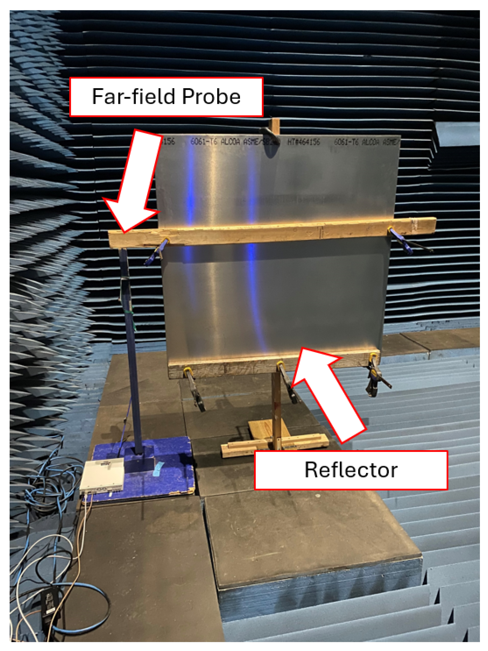
3. Data Collection II: Stationary Target Reflection

In this section, we show the results from a binary target detection test of a stationary target performed in an anechoic chamber. The reflector used during this collection is a $1.22\mathrm{m}\times 1.22\mathrm{m}$ flat aluminum sheet stabilized with wooden boards that were adjusted using two laser pointers so that the bowing across the sheet was less than 6.4 mm ($1/4$ in). The block diagram of the system is shown in Figure 1, and photographs of the experimental setup inside the chamber are shown in Figure 5 (transmit/receive system) and Figure 6 (reflector).

3.1. Signal Model at the Target

General target behavior can be modeled as a Doppler shift $e^{j2\pi {\nu }_{n}t}$ with a fast-time varying amplitude ${\sigma }_n\left(t\right)$, where ${\nu }_n=2v{f}_n/c$ is the Doppler shift caused by a target with radial velocity v and ${\sigma }_n\left(t\right)$ is the fast-time amplitude of the target reflection at fast-time t. The target behavior is incorporated into Equation (1) as

$$F_{tgt}(t;R_t,{\theta }_t)=\sum _{n=0}^{N-1}{\sigma }_n\left(t\right)e^{j2\pi {\nu }_{n}t}{e}^{j2\pi f_n(t-R_n/c)}.$$

(7)

3.2. Signal Model at the Receiver

Since the maximum bandwidth generated by our operating parameters $B(N-1)=20\mathrm{kHz}·2=40\mathrm{kHz}\ll f_0$, we can simplify Equation (7) using the monochromatic assumption. Furthermore, we assume that the target radar cross section (RCS) is relatively constant during each sampling period, i.e., ${\sigma }_n\left(t\right)\approx 1$. Under these assumptions, the received baseband signal model for a target at $(R,\theta )=(R_t,{\theta }_t)$ is

$$\begin{array}{cc}\hfill F_{R,bb}& (t;R_t,{\theta }_t)=\hfill \\ \hfill & e^{j2\pi {\nu }_{0}t}·\left[\sum _{n=0}^{N-1}{e}^{j2\pi n\Delta ft}·e^{-j2\pi f_0(R_n+R_r)/c)}\right],\hfill \end{array}$$

(8)

where $R_r$ is the common distance from the target to the receive probe.

3.3. Matched Filter Threshold and Receive Antenna Shielding

The matched filter (MF) for our experimental setup is the convolution of the received signal with the Tx copy created using RF hardware (see Figure 1). Mathematically, this is represented as [47]

$$s_{MF}\left(t\right)={\int }_{-\infty }^{+\infty }{F}_{R,bb}\left(\tau \right)F_{Copy}(t-\tau )d\tau ,$$

(9)

where

$$F_{Copy}\left(t\right)=\sum _{n=0}^{N-1}{e}^{j2\pi n\Delta ft}.$$

(10)

In this quasi-monostatic transmit/receive setup, we expect some level of sidelobe leakage from the transmit array to the receive antenna; therefore, we constructed a septum with an embedded aluminum sheet to shield the receive antenna. The MF threshold is then set by taking the MF response when the transmitters are on and no target is present.

Ettus Research documentation states that the UBX-160 daughterboard has an experimentally determined minimum discernible signal (MDS) level of −135 dBm in the HF band [48]. We empirically find the MDS level (−65 dBm) inside the chamber by taking interference plus noise measurements with the transmitters on, then sampling input tones with decreasing power until the amplitude falls below the interference plus noise level. Assuming a lossless system, a 0 dBsm target yields a maximum detectable range $R_{max}=15.9\mathrm{m}$ found using the radar range equation

$$R_{max}={\left[N·{\displaystyle \frac{P_t{G}_t{G}_r{\lambda }_0^2·\sigma }{{\left(4\pi \right)}^3{P}_r}}\right]}^{1/4},$$

(11)

with number of elements $N=3$, transmit power at each transmit antenna terminal $P_t=14.7\mathrm{dBm}$, transmit and receive antenna gains $G_t=G_r=6.5\mathrm{dB}$, RCS $\sigma =0\mathrm{dBsm}$, and receive power $P_r=-65\mathrm{dBm}$. Note that the preceding system parameters are given in a decibel (dB) scale but are converted to a linear scale when calculating $R_{max}$. Thus, the number of elements N in Equation (11) accounts for the linear scaling of the transmit power and the cascaded transmit/receive gains that occur when $N>1$.

3.4. Target Detection Test Criteria

We rule a successful target detection as satisfying a negative-positive-negative (neg-pos-neg) test. In this test, the MF is first computed without the presence of a target. This constitutes a negative target detection and sets the MF threshold for the positive test. A reflector (Figure 6) is then placed broadside to the transmit array at a nominal distance in the far field, and the MF response is calculated. A positive target detection requires that the maximum of the MF be at least 3 dB higher than the threshold set in the preceding negative test. The target is removed and the MF is calculated again. The maximum of the MF should again be approximately equal to the threshold set during the first negative test.

3.5. Binary Target Detection: Experimental Results

The test results are split into the received target echo and its associated MF response. We use a flat plate reflector to produce a single reflection observed at the receiver. This reflector choice is made purposefully to verify that the theoretical fast-time behavior of the target echo matches the work of Bang in [49].

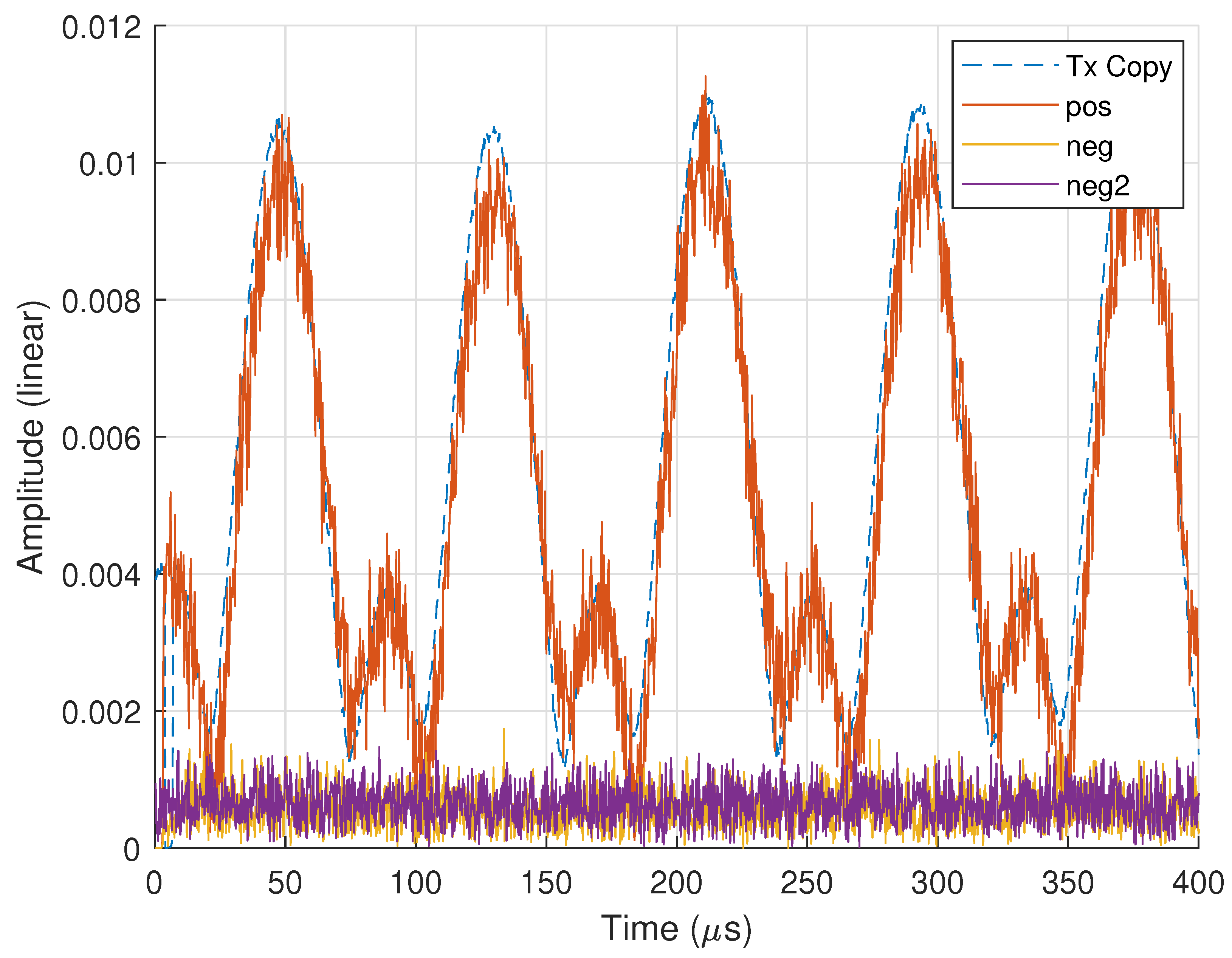
3.5.1. Target Echo

We take measurements of the target echo from the locations $(R,\theta )=$ (3.35 m, 0°), (6.70 m, 0°) and show the results for the latter in Figure 7. The captured target echo (solid) matches well with the copy of the transmitted waveform (dashed), demonstrating that the experimental fast-time RCS behavior agrees well with [49]. Also included in Figure 7 is the interference plus noise sample data, providing a visual representation of the neg-pos-neg test in Section 3.4.

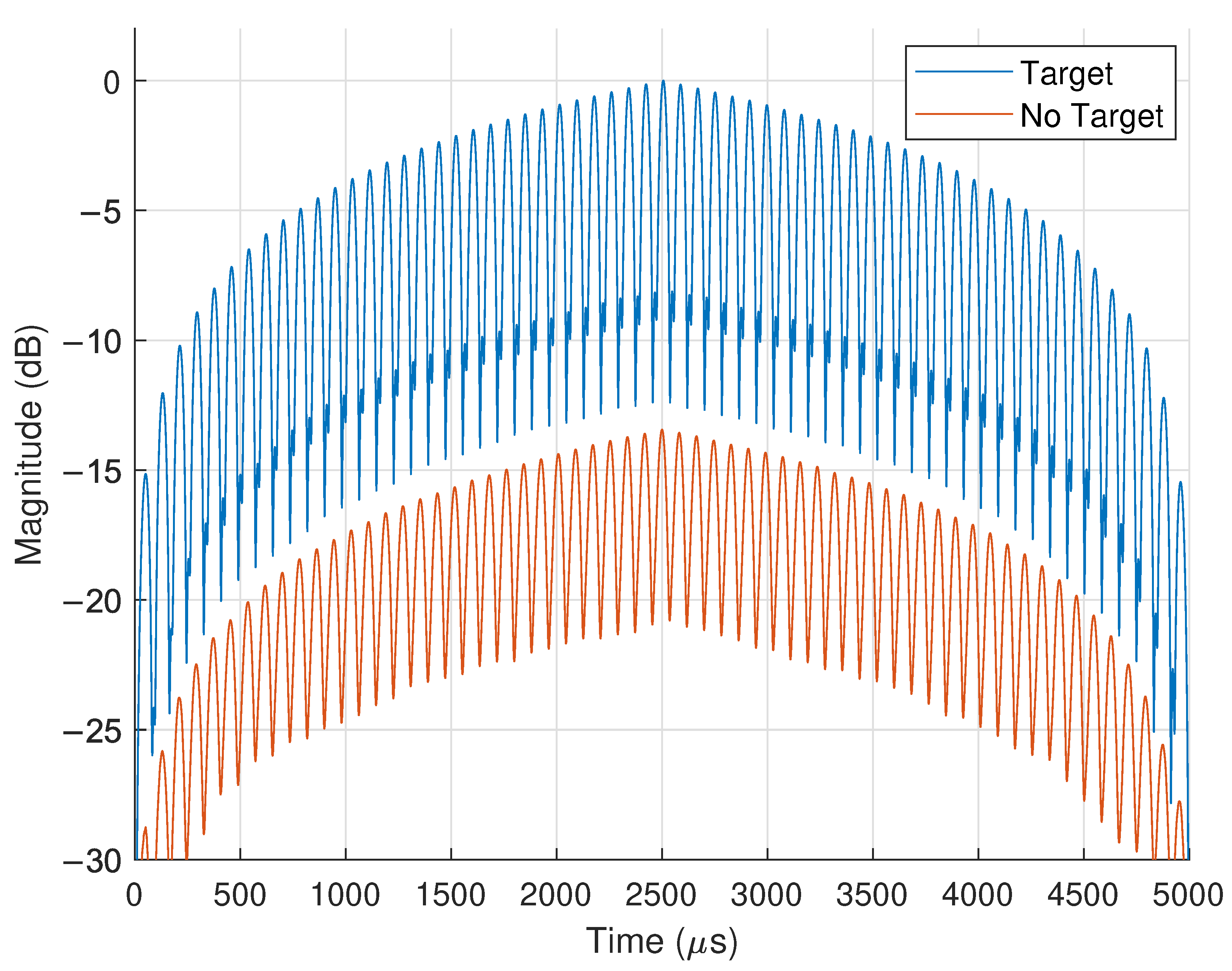
3.5.2. MF Response

As can be seen from Figure 7, there is a stark contrast between the sampled data with and without the presence of a target in the far field; thus, as expected, the MF responses closely follow the sampled data from the receive antenna. Figure 8 shows the binary target detection MF response calculated using Equation (9) at $(R,\theta )=$ (6.70 m, 0°). There exist differences of approximately 13.2 dB and 13.4 dB, respectively, between the MF responses of the positive and negative tests at this location. These increases in MF strongly suggest the presence of a target in the far field when compared to the cases when no target is present.

4. Data Collection III: Moving Targets

In this section, we capture the response from two moving targets: one car and one drone. The block diagram for the setup is shown in Figure 9, and the corresponding photographs are shown in Figure 10 and Figure 11, respectively. The maximum detectable range of a $0\mathrm{dBsm}$ target for this test is $R_{max}=8.34\mathrm{m}$, found by evaluating Equation (11) with $N=2$ and the minimum receive power $P_r=-55\mathrm{dBm}$. Target sampling occurs at an approximate range of $R=6.1\mathrm{m}$ and $R=2.43\mathrm{m}$ for the car and the drone, respectively. During the drone collection, the drone followed a direct line-of-sight trajectory along boresight during both collections. The drone was flown as close to a constant height as possible, yielding a radial velocity living mostly in the range–angle plane of the radar.

4.1. Theoretical Frequency Domain Response

We use the Fourier relationships [50]

$$\begin{array}{cc}\hfill e^{\pm j{\omega }_{0}t}& \iff 2\pi \delta (\omega \mp {\omega }_0)\hfill \\ \hfill \mathcal{F}\left(e^{j({\omega }_{0}t\pm \theta )}\right)& =e^{\pm j\theta }\mathcal{F}\left(e^{j{\omega }_{0}t}\right)\hfill \end{array}$$

(12)

to find the expected frequency response at the receiver. Since the Fourier transform is a linear operation, we can take the Fourier transform of each individual term in Equation (8), then sum the individual responses, to obtain the overall response of the system. This is expressed mathematically as

$$\begin{array}{cc}\hfill \mathcal{F}\left[F_{R,bb}(t;R,\theta )\right]& =\mathcal{F}\left[\sum _{n=0}^{N-1}{e}^{j{\omega }_{n}t}·e^{-j{\theta }_n}\right]\hfill \\ \hfill & =\sum _{n=0}^{N-1}\mathcal{F}\left[e^{j{\omega }_{n}t}·e^{-j{\theta }_n}\right],\hfill \end{array}$$

(13)

where ${\omega }_n=2\pi (n\Delta f+{\nu }_0)$ and ${\theta }_n=2\pi f_0(R_n+R_r)/c)$. Using the Fourier relationships from Equation (12) in conjunction with Equation (13), the total response is then

$$\mathcal{F}\left(\omega \right)=2\pi \sum _{n=0}^{N-1}\delta (\omega -{\omega }_n)·e^{-j2\pi {\theta }_n}.$$

(14)

Note that Equation (14) assumes no stationary clutter exists in the receive echo from the target. In practice, stationary mainlobe clutter will exist at each radiated frequency, with the target Doppler response following Equation (14).

4.2. Frequency Bin Resolution

The frequency resolution of the fast Fourier transform (FFT) is

$$\Delta f={\displaystyle \frac{f_s}{N_s}}\left(\mathrm{Hz}\right),$$

(15)

where $f_s$ is the sampling frequency and $N_s$ is the number of samples. The Potensic T25 Drone has a maximum speed of $6.94\mathrm{m}/\mathrm{s}$. Thus, we capture more samples for better frequency resolution at lower Doppler shifts. Using Equation (15) above, the frequency resolutions of our two collections are

$$\begin{array}{cc}\hfill \Delta f_{vehicle}& ={\displaystyle \frac{2.5\mathrm{MHz}}{250,000\mathrm{samples}}}=10\mathrm{Hz}\hfill \\ \hfill \Delta f_{drone}& ={\displaystyle \frac{2.5\mathrm{MHz}}{300,000\mathrm{samples}}}=8.33\mathrm{Hz}\hfill \end{array}.$$

(16)

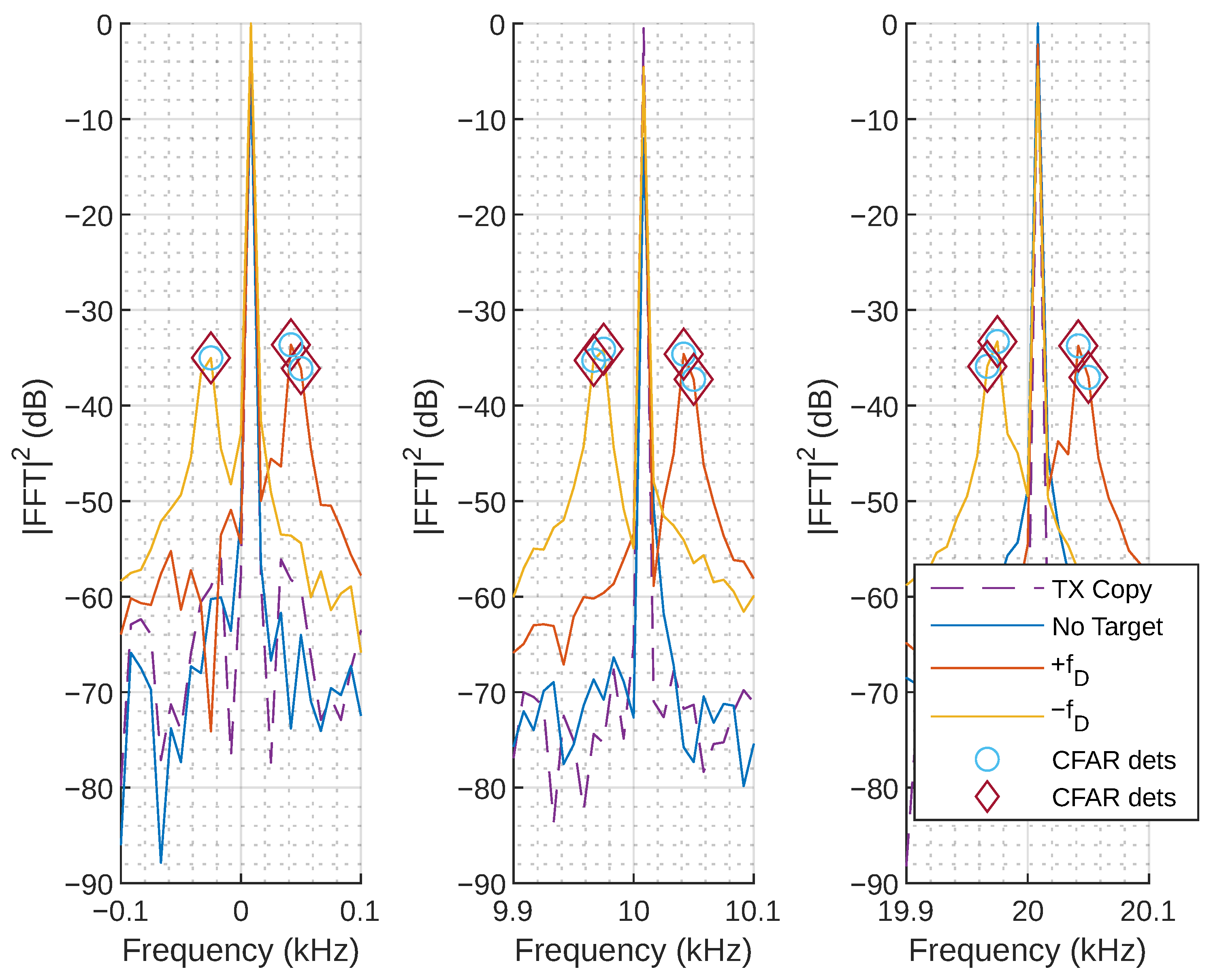
4.3. Experimental Results

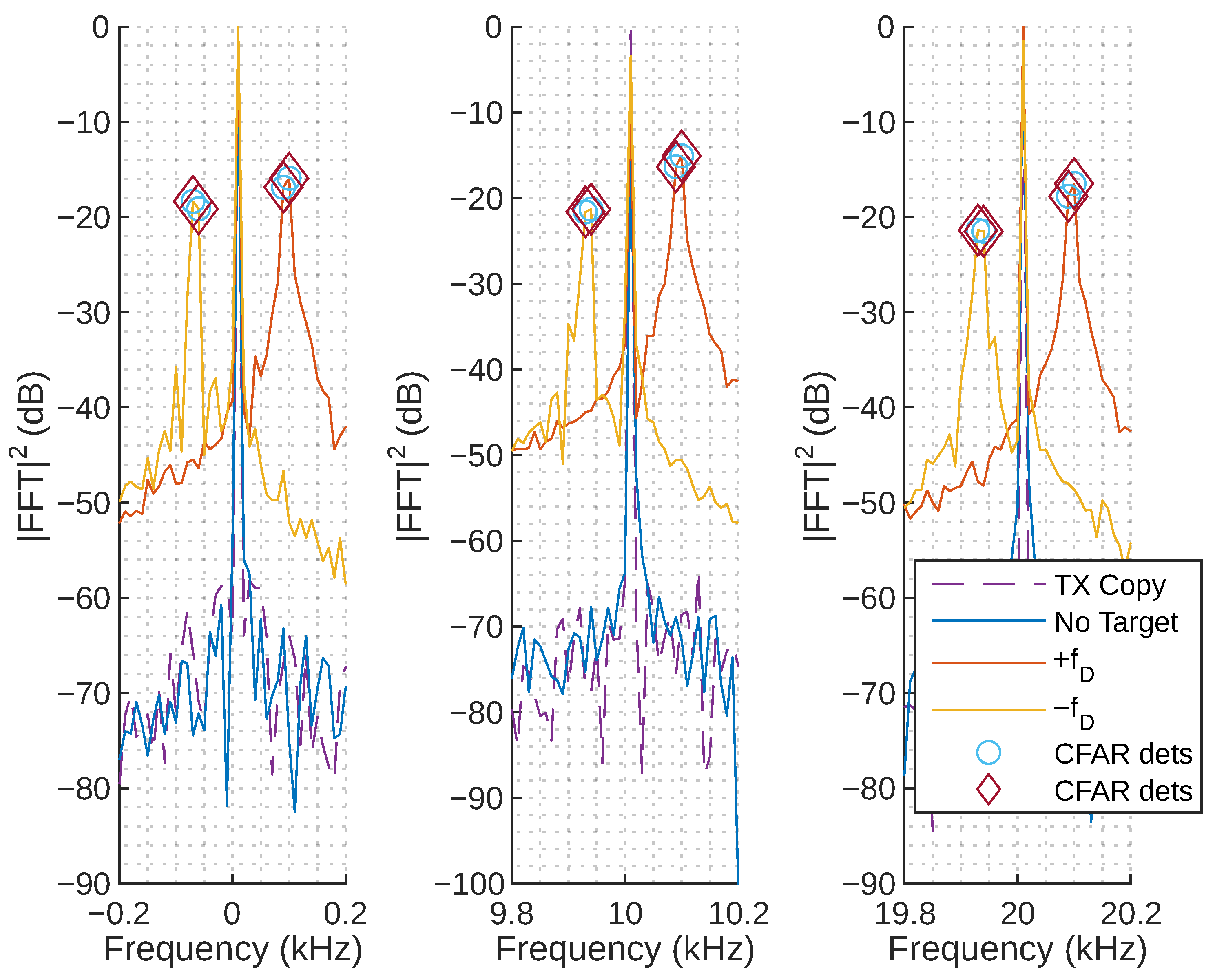
4.3.1. Frequency Domain Response

The frequency response from the captured moving vehicle data and drone data is shown in Figure 12 and Figure 13, respectively. The information displayed in the legends of Figure 12 and Figure 13 is as follows:

• TX Copy: FFT of the captured analog signal created using RF hardware.
• No Target: FFT of the captured experimental scene with no targets present.
• $+f_D$: FFT of the data captured from a target moving toward the radar.
• $-f_D$: FFT of data captured from a target moving away from the radar.
• CFAR dets: cell averaging (CA)-constant false alarm rate (CFAR) detections (see Section 4.3.3).

4.3.2. Radial Velocity

The radial velocity of a target can be found by rearranging the well-known expression for Doppler shift:

$$v={\displaystyle \frac{c{\nu }_0}{2f_0}}.$$

(17)

The value of ${\nu }_0$ is assumed to be the midpoint of the frequency bin containing the Doppler peak referenced with the midpoint of the frequency bin containing the peak of the TX Copy FFT. The radial velocities from the Doppler information in Figure 12 and Figure 13 are given in

Table 5. Radial velocities calculated from the Doppler shifts shown in Figure 12 and Figure 13.

Test	Radial Motion	$|{\mathit{v}}_{\mathbf{measured}}|\mathbf{m}/\mathbf{s}$	$|{\mathit{v}}_{\mathbf{true}}|$ m/s
Car	$+{\nu }_0$	6.37	6.71
Car	$-{\nu }_0$	5.62	6.26
Drone	$+{\nu }_0$	2.81	3.13
Drone	$-{\nu }_0$	2.81	3.13

, along with the true radial velocities of each test.

4.3.3. CA-CFAR Detection

CFAR is a statistical target detection technique that uses adaptive thresholding with a sliding window approach to detect targets while maintaining a consistent false alarm rate. Our scene background is an open area and is assumed to be homogeneous. This assumption is supported by the “No Target” curves in Figure 12 and Figure 13, which display a uniform background outside of the stationary reflections at the carrier frequencies $f_n$.

From ([51] Chapter 16.5), the maximum likelihood estimate of the interference power ${\widehat{\sigma }}_i^2$, the CA-CFAR constant ${\alpha }_{CA}$, and the CA-CFAR threshold $T_{CA}$ are defined as

$${\widehat{\sigma }}_i^2=\sum _{m=1}^M{z}_m,$$

(18)

$${\alpha }_{CA}=(P_{fa}^{-1/M}-1),\mathrm{and}$$

(19)

$$T_{CA}={\alpha }_{CA}{\widehat{\sigma }}_i^2,$$

(20)

respectively, where the test cells $z_m$ are indexed from $m=1,2,...,M$ with M total test cells, and $P_{fa}$ is the desired probability of false alarm for the detector.

Overlaid in Figure 12 and Figure 13 are CA-CFAR detections. We use $M=16$ total test cells, $P_{fa}={10}^{-6}$, and two guard cells on each side of the cell under test. We notch out $\pm 10\mathrm{Hz}$ on either side of the zero-Doppler frequencies to suppress stationary scene clutter. The zero-Doppler frequencies are found via the peaks of the “TX Copy” curves.

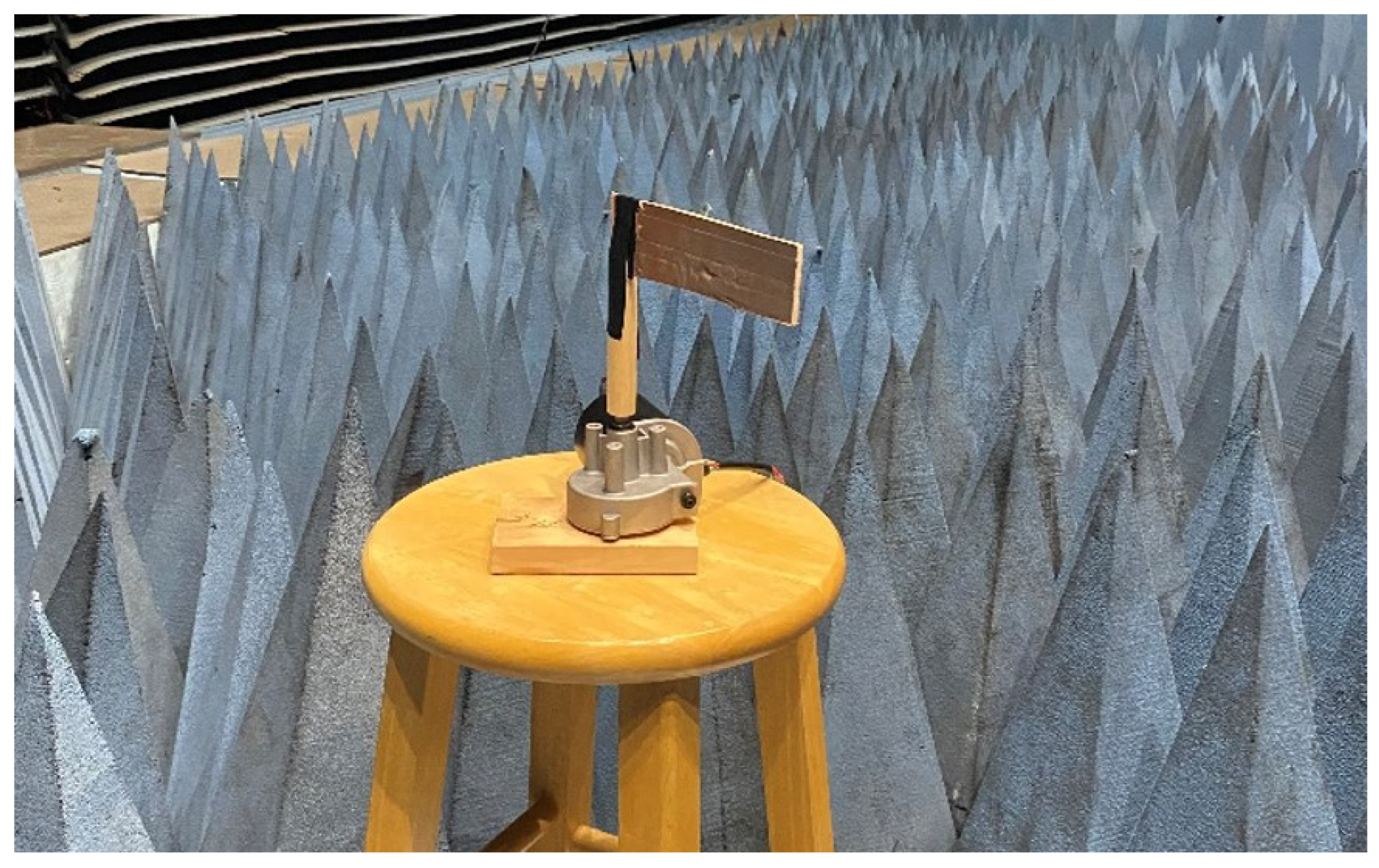
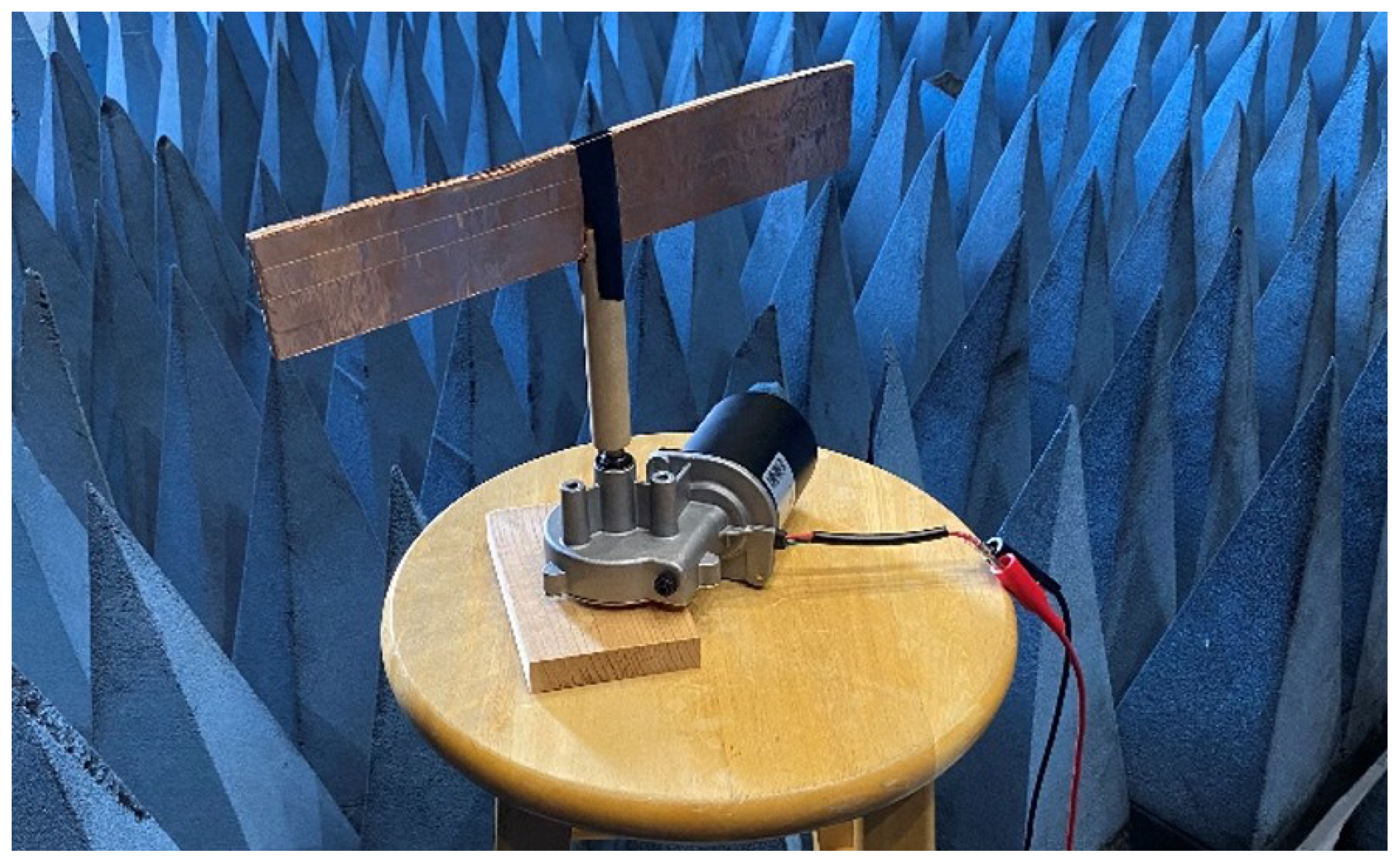
5. Data Collection IV: Micro-Doppler

In this section, we present time–frequency analysis of micro-Doppler data collected using a system whose diagram is shown in Figure 14. We construct two rotating blade apparatuses (a single-blade apparatus in Figure 15 and a two-blade apparatus in Figure 16) that are driven by a single-speed 12 V DC motor to generate reflections. The maximum detectable range of a $0\mathrm{dBsm}$ target for this test is $R_{max}=8.34\mathrm{m}$, found by evaluating Equation (11) with the minimum receive power $P_r=-65\mathrm{dBm}$.

5.1. Signal Model

The signal model for the fast-time micro-Doppler response from the setup in Figure 14 is adopted from [52,53,54] and is given as

$$\begin{array}{c}\hfill F_{mD}(t;R_b)=\sum _{n=0}^{N-1}\sum _{k=0}^{K-1}L{e}^{j(2\pi f_{n}t-{\displaystyle \frac{4\pi }{{\lambda }_0}}(R_b+{\displaystyle \frac{L}{2}}sin(\Omega t+{\displaystyle \frac{2\pi k}{K}}))}\\ \hfill ·\sin \mathrm{c}\left({\displaystyle \frac{4\pi }{{\lambda }_0}}{\displaystyle \frac{L}{2}}sin(\Omega t+{\displaystyle \frac{2\pi k}{K}})\right),\end{array}$$

(21)

where K is the number of blades, $R_b$ is the range to the center of rotation, $\Omega (\mathrm{rad}/\mathrm{s})$ is the frequency of rotation, and $L_{Kb}$ is the blade length for a system with b total blades. Note the use of $f_n$ and monochromatic assumption for wavelength in Equation (21).

The maximum theoretical micro-Doppler shift is adopted from [52] as

$$f_{mD}={\displaystyle \frac{2\Omega L_{Kb}}{{\lambda }_n}}\approx {\displaystyle \frac{2\Omega L_{Kb}}{{\lambda }_0}}.$$

(22)

5.2. Experimental Operating Parameters

We perform the single-blade collection at a radial distance of $R_b=1.52\mathrm{m}$ (Collection IVa) and the double-blade collection at a radial distance of $R_b=3.51$ (Collection IVb), respectively. The one-blade apparatus has a blade length $L_{1b}=0.165\mathrm{m}$, and the two-blade apparatus has two blades with equal lengths $L_{2b}=0.145\mathrm{m}$. The sampling rate for this collection is $f_s=1\mathrm{MHz}$ with a collection time of $10\mathrm{seconds}$ (${10}^6$ total samples). During both collections, the quasi-monostatic transmit/receive setup and blade mount are both stationary; the only movement occurring is/are the rotating blade(s). Additionally, we assume that $\theta \approx 0$ since $R_b$ is much larger than the spacing between the transmit array and receive antenna. A photograph of the transmit-receive setup is shown in Figure 17.

To generate a larger micro-Doppler shift, we increase the carrier frequency from $f_0=2\mathrm{GHz}$ to $f_0=5.90\mathrm{GHz}$, which is near the upper limit ($6\mathrm{GHz}$) of the TwinRX operational frequency range. Due to long data streaming times, host PC limitations cause a substitution of CW signal generators as the transmit hardware. The X310 with a TwinRX daughterboard is used to sample the signal from the receive antenna.

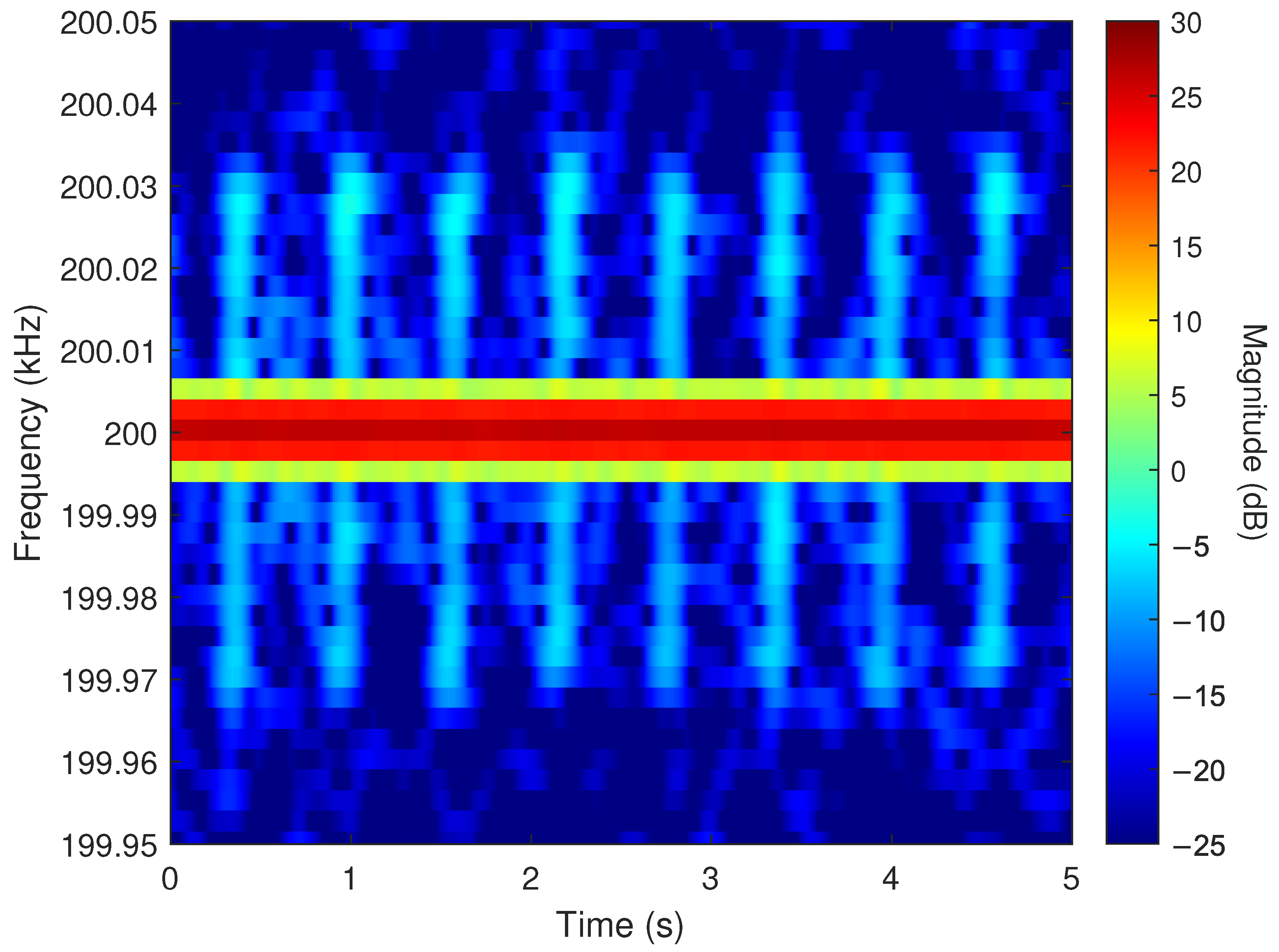
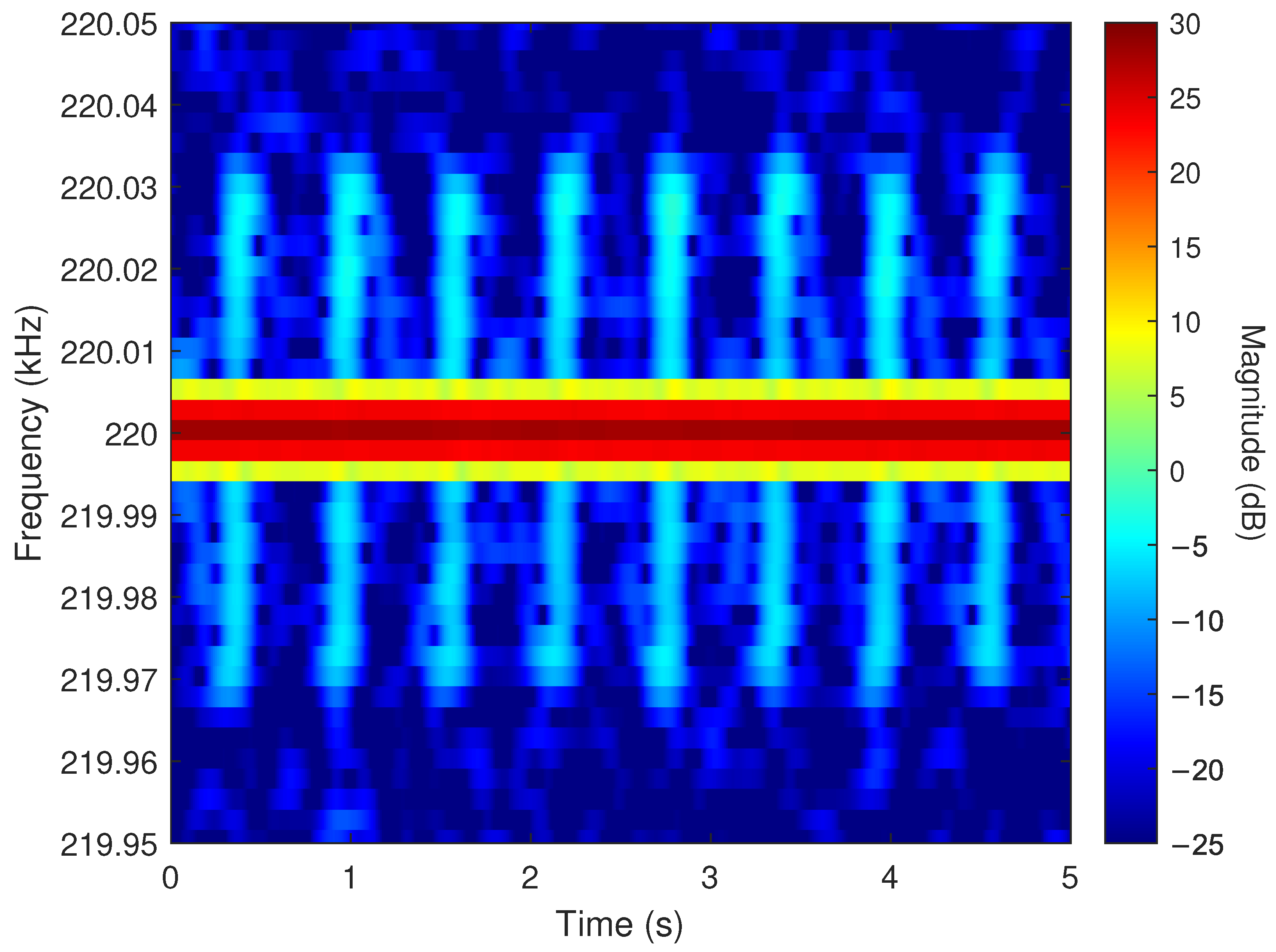
5.3. Time–Frequency Analysis of Simulated Reflections

We use the short-time Fourier transform (STFT), a linear time–frequency analysis method, to analyze the received samples. Linear time–frequency analysis is selected for its ease of interpretation, as it lacks the cross-terms found in bilinear time–frequency analysis methods [55,56].

The STFT is defined as [55,56]

$$X(t,f)={\int }_{-\infty }^{+\infty }x\left(\tau \right)h(\tau -t)e^{-j2\pi f\tau }d\tau ,$$

(23)

where $x(·)$ is the captured signal, $h(·)$ is the window function, and f is frequency of the Fourier kernel.

Our Fourier transform (FT) window is a $400·{10}^3\mathrm{sample}$ Blackman window, and the sample overlap between successive FT windows is $10·{10}^3\mathrm{samples}$. These parameters yield time and frequency resolutions of, respectively, $t_{res}\approx 0.40\mathrm{s}$ and $f_{res}=2.5\mathrm{Hz}$.

Time–frequency analysis of the simulated fast-time micro-Doppler return is shown in Figure 18 through Figure 19. The simulations use the operational parameters given above in Section 5.2. A $5\mathrm{second}$ zoom in is shown to provide a clearer view of key time–frequency features produced by the rotating blade(s):

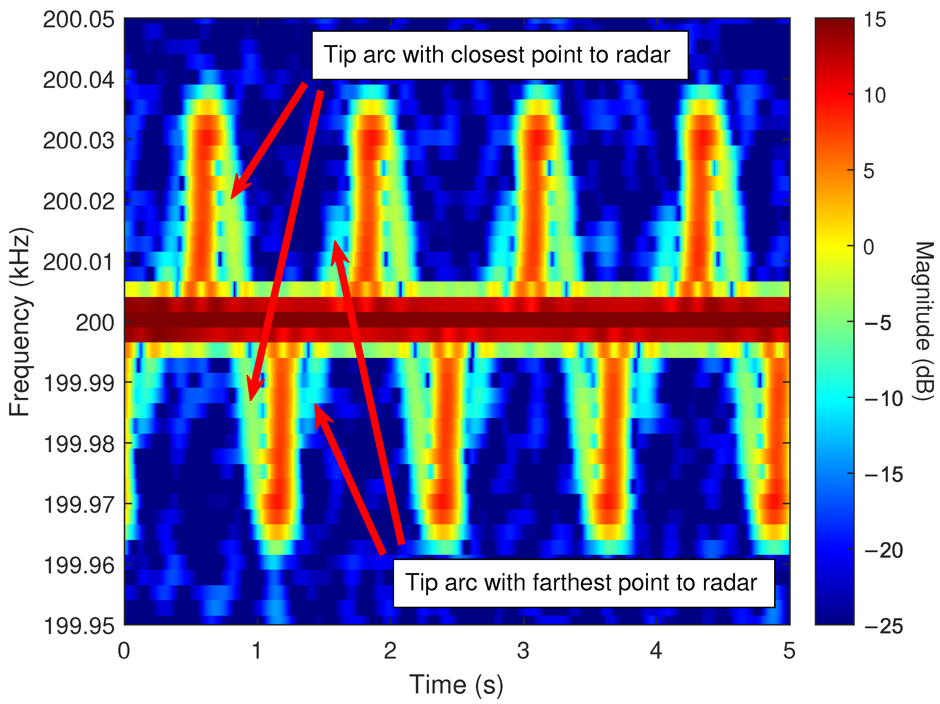
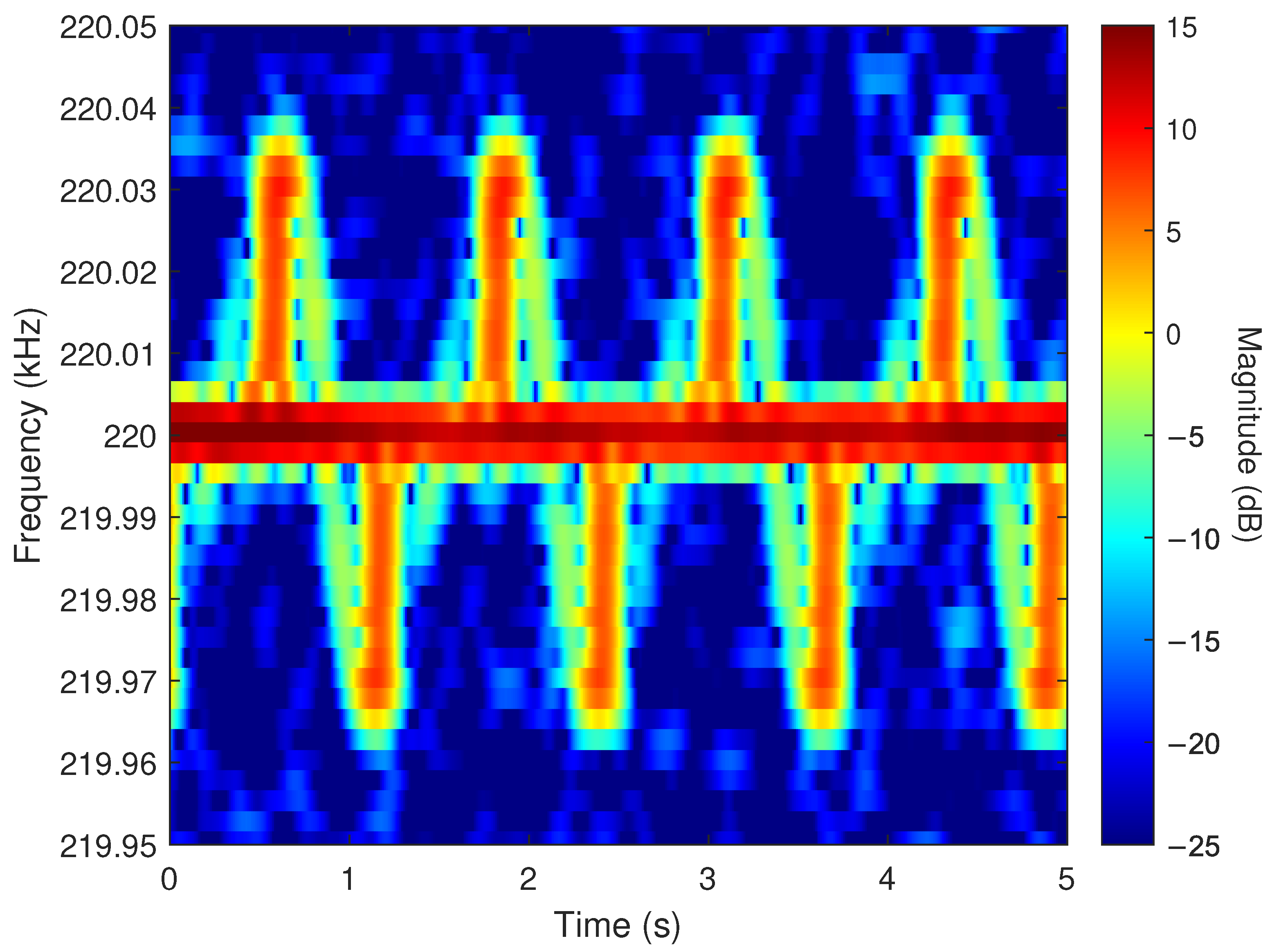
• Periodic blade flashes.
• Strong scattering from the blade tip during each periodic flash.
• A sinusoidal trace produced by the tip of the rotating blade.

The enumerated items above are annotated in Figure 18 to provide a link between the verbal description and the associated time–frequency behavior. Note the similarity between Figure 18, Figure 20 and Figure 19, Figure 21, with Figure 19, Figure 21 being the summation of Figure 18, Figure 20 and a 180° phase-shifted version of Figure 18, Figure 20, respectively.

5.4. Experimental Results

Single-Blade Collection

The time–frequency analysis of the single-blade collection is shown in Figure 22 and Figure 23. Figure 22 and Figure 23 both exhibit periodic blade flashes, strong scattering from the blade tip, and a sinusoidal trace produced by the tip of the rotating blade. Note that the sinusoidal trace produced by the tip of the rotating blade, while present throughout each rotation, is more intense when the blade is at its closest point to the radar. This effect is annotated in Figure 22.

5.5. Two-Blade Collection

The time–frequency analysis of the two-blade collection is shown in Figure 24 and Figure 25. Figure 24 and Figure 25 both exhibit periodic blade flashes and strong scattering from the blade tip, but lack the prominent sinusoidal ‘tip trace’ seen in Figure 22 and Figure 23. This is expected because of the increased collection distance.

5.6. Predicted Propeller Length

Following the procedure in [57], the length of the rotating propeller blades can be estimated. First, Equation (22) is rearranged as follows

$$L_{Kb}={\displaystyle \frac{{\lambda }_0{f}_{mD}}{2\Omega }}$$

(24)

Using Equation (24) in conjunction with the experimentally measured values of $f_{mD,max}$, the predicted propeller lengths from all of the collections are shown in

Table 6. Estimated (est) and calculated (calc) propeller blade length comparison. Note (meas) and (sys) represent experimentally measured and implemented system parameters, respectively.

${\mathit{K}}^{\mathit{sys}}$ (# of Blades)	${\mathit{\lambda }}_0^{\mathit{sys}}$ (m)	${\mathbf{\Omega }}^{\mathit{sys}}$ (rad/s)	${\mathit{L}}_{\mathit{Kb}}^{\mathit{sys}}$ (m)	${\mathit{f}}_{\mathit{mD}}^{\mathit{calc}}$ (Hz)	${\mathit{f}}_{\mathit{mD}}^{\mathit{meas}}$ (Hz)	${\mathit{L}}_{\mathit{Kb}}^{\mathit{est}}$ (m)
1	0.0508	5.24	0.165	34	36	0.175
2	0.0508	5.24	0.145	29.8	32	0.155

.

6. Concluding Remarks

In this work, we present the data collected from four different experimental test setups of a linear CW FDA radar, with an emphasis on the signal-model-level agreement between theoretical analysis and experimental results. These collections also showcase the potential utility of the FDA as a low-complexity perimeter surveillance system with an auto-scanning mainbeam feature.

We experimentally demonstrated the following:

• Two key attributes of far-field pattern: temporal periodicity and angular scanning behavior of the mainbeam.
• Basic radar capabilities through binary target detection tests in a controlled anechoic environment.
• Doppler shift from two moving targets: a car and a drone.
• Extraction of micro-Doppler features from rotating blades using the STFT as a tool for time–frequency analysis.

In conjunction with our work in [31], where we capture the fast-time response of a linear FDA using fast-time binary phase-shift keying (BPSK) modulations at each element, this collective body of work provides a solid experimental exploration of the linear FDA at the signal model level.

Future work in this area would see an expansion of the current system into larger linear arrays, as well as planar array architectures, to experimentally capture fast-time behaviors from advanced FDA frequency offset schemes and array architectures (see Section 1) often seen in the academic literature.

In this work, differences can be seen in the experimental and theoretically expected values. Sources of experimental error include SDR phase noise, hardware timing mismatch, and non-ideal antenna locations. Thus, sensitivity studies are also pertinent next steps in the evolution of this research thrust. Existing motivation for such work can be found in [10,11,58,59], where FDA manifold sensitivity, beampattern sensitivity due to frequency offset error, and phase noise sensitivity are studied. The theoretical analysis can be extended with data collections and subsequent analysis and study using different FDA transmit/receive architectures.

References

- Antonik, P.; Wicks, M.; Griffiths, H.; Baker, C. Frequency Diverse Array Radars. In Proceedings of the 2006 IEEE Conference on Radar, Verona, NY, USA, 24–27 April 2006; pp. 215–217. [Google Scholar] [CrossRef]
- Antonik, P.; Wicks, M.C.; Griffiths, H.D.; Baker, C.J. Range dependent beamforming using element level waveform diversity. In Proceedings of the 2006 InternationalWaveform Diversity & Design Conference, Lihue, HI, USA, 22–27 January 2006; pp. 1–6. [Google Scholar] [CrossRef]
- Antonik, P.; Wicks, M.; Griffiths, H.; Baker, C. Multi-mission multi-mode waveform diversity. In Proceedings of the 2006 IEEE Conference on Radar, Verona, NY, USA, 24–27 April 2006; pp. 580–582. [Google Scholar] [CrossRef]
- Secmen, M.; Demir, S.; Hizal, A.; Eker, T. Frequency diverse array antenna with periodic time modulated pattern in range and angle. In Proceedings of the 2007 IEEE Radar Conference, Waltham, MA, USA, 17–20 April 2007; pp. 427–430. [Google Scholar] [CrossRef]
- Huang, J.; Tong, K.F.; Baker, C. Frequency diverse array with beam scanning feature. In Proceedings of the 2008 IEEE Antennas and Propagation Society International Symposium, San Diego, CA, USA, 5–11 July 2008; pp. 1–4. [Google Scholar] [CrossRef]
- Liu, Y.; Ruan, H.; Wang, L.; Nehorai, A. The random frequency diverse array: A new antenna structure for uncoupled direction-range indication in active sensing. IEEE J. Sel. Top. Signal Process. 2017, 11, 295–308. [Google Scholar] [CrossRef]
- Wang, W.Q. Subarray-based frequency diverse array radar for target range-angle estimation. IEEE Trans. Aerosp. Electron. Syst. 2014, 50, 3057–3067. [Google Scholar] [CrossRef]
- Wang, W.Q.; So, H.C. Transmit subaperturing for range and angle estimation in frequency diverse array radar. IEEE Trans. Signal Process. 2014, 62, 2000–2011. [Google Scholar] [CrossRef]
- Xu, Y.; Shi, X.; Xu, J.; Huang, L.; Li, W. Range–angle-decoupled beampattern synthesis with subarray-based frequency diverse array. Digit. Signal Process. 2017, 64, 49–59. [Google Scholar] [CrossRef]
- Correll, B.; Rigling, B. Quantized, power law frequency diverse arrays. In Proceedings of the 2023 IEEE Radar Conference (RadarConf23), San Antonio, TX, USA, 1–5 May 2023; pp. 1–6. [Google Scholar]
- Correll, B.; Rigling, B. Auto-scanning quantized, power law frequency diverse arrays. In Proceedings of the 2024 IEEE Radar Conference (RadarConf24), Denver, CO, USA, 6–10 May 2024. [Google Scholar]
- Khan, W.; Qureshi, I.M.; Saeed, S. Frequency diverse array radar with logarithmically increasing frequency offset. IEEE Antennas Wirel. Propag. Lett. 2015, 14, 499–502. [Google Scholar] [CrossRef]
- Gao, K.; Wang, W.Q.; Cai, J.; Xiong, J. Decoupled frequency diverse array range-angle-dependent beampattern synthesis using non-linearly increasing frequency offsets. IET Microwaves Antennas Propag. 2016, 10, 880–884. [Google Scholar] [CrossRef]
- Mahmood, M.; Mir, H. Frequency diverse array beamforming using nonuniform logarithmic frequency increments. IEEE Antennas Wirel. Propag. Lett. 2018, 17, 1817–1821. [Google Scholar] [CrossRef]
- Liao, Y.; Wang, W.Q.; Zheng, Z. Frequency diverse array beampattern synthesis using symmetrical logarithmic frequency offsets for target indication. IEEE Trans. Antennas Propag. 2019, 67, 3505–3509. [Google Scholar] [CrossRef]
- Shao, H.; Dai, J.; Xiong, J.; Chen, H.; Wang, W.Q. Dot-shaped range-angle beampattern synthesis for frequency diverse array. IEEE Antennas Wirel. Propag. Lett. 2016, 15, 1703–1706. [Google Scholar] [CrossRef]
- Xiong, J.; Wang, W.Q.; Shao, H.; Chen, H. Frequency diverse array transmit beampattern optimization with genetic algorithm. IEEE Antennas Wirel. Propag. Lett. 2016, 16, 469–472. [Google Scholar] [CrossRef]
- Geng, L.; Li, Y.; Dong, L.; Tan, Y.; Cheng, W. Efficiently Refining Beampattern in FDA-MIMO Radar via Alternating Manifold Optimization for Maximizing Signal-to-Interference-Noise Ratio. Remote Sens. 2024, 16, 1364. [Google Scholar] [CrossRef]
- Hsin, C.L.; Kiang, J.F. Frequency-Hopping Frequency-Diverse MIMO Radar for Target Detection and Localization Under False-Target Jamming. IEEE Access 2023, 11, 62121–62139. [Google Scholar] [CrossRef]
- Abdalla, A.; Abdalla, H.; Ramadan, M.; Mohamed, S.; Bin, T. Overview of frequency diverse array in radar ECCM applications. In Proceedings of the 2017 International Conference on Communication, Control, Computing and Electronics Engineering (ICCCCEE), Khartoum, Sudan, 16–18 January 2017; pp. 1–9. [Google Scholar] [CrossRef]
- Yao, A.M.; Anselmi, N.; Rocca, P. A multi-carrier frequency diverse array design method for wireless power transmission. In Proceedings of the 12th European Conference on Antennas and Propagation (EuCAP 2018), London, UK, 9–13 April 2018; pp. 1–4. [Google Scholar] [CrossRef]
- Wang, W.Q. Retrodirective frequency diverse array focusing for wireless Information and power transfer. IEEE J. Sel. Areas Commun. 2019, 37, 61–73. [Google Scholar] [CrossRef]
- Fazzini, E.; Shanawani, M.; Costanzo, A.; Masotti, D. A logarithmic frequency-diverse array system for precise wireless power transfer. In Proceedings of the 2020 50th European Microwave Conference (EuMC), Utrecht, Netherlands, 12–14 January 2021; pp. 646–649. [Google Scholar]
- Antonik, P. An Investigation of a Frequency Diverse Array. PhD Thesis, UCL (University College London), London, UK, 2009. [Google Scholar]
- Brady, S.H. Frequency Diverse Array Radar: Signal Characterization and Measurement Accuracy. Masters Thesis, Air Force Institute of Technology, Dayton, OH, USA, 2012. [Google Scholar]
- Eker, T. A Conceptual Evaluation of Frequency Diverse Arrays and Novel Utilization of LFMCW. Ph.D. Thesis, Middle East Technical University, Ankara, Turkey, 2011. [Google Scholar]
- Çetintepe, C. Analysis of Frequency Diverse Arrays for Radar and Communication Applications. Ph.D. Thesis, Middle East Technical University, Ankara, Turkey, 2015. [Google Scholar]
- McCormick, P.M.; Jones, A.; Kellerman, N.; Mathieu, B.; Mertz, A. Experimental demonstration of a low-complexity multiple-input single-output frequency diverse array framework. In Proceedings of the 2023 IEEE Radar Conference (RadarConf23), Sydney, Australia, 6–10 November 2023; pp. 1–6. [Google Scholar]
- Kellerman, N. A MISO Frequency Diverse Array Implementation. Master’s Thesis, University of Kansas, Lawrence, KS, USA, 2023. [Google Scholar]
- Munson, N.R.; Correll, B.; Narayanan, R.M.; Bufler, T.D. Experimental Test of a Frequency Diverse Array Radar Target Detection System Using SDRs: Preliminary Results. In Proceedings of the 2024 IEEE Radar Conference (RadarConf24), Denver, CO, USA, 6–10 May 2024; pp. 1–6. [Google Scholar] [CrossRef]
- Munson, N.R.; Correll Jr, B.; Henry, J.K.; Narayanan, R.M.; Bufler, T.D. Design and Implementation of a Binary Phase-Shift Keying Frequency Diverse Array: Considerations and Challenges. Sensors 2025, 25, 193. [Google Scholar] [CrossRef] [PubMed]
- Huang, J.; Tong, K.F.; Baker, C. Frequency diverse array: Simulation and design. In Proceedings of the 2009 Loughborough Antennas & Propagation Conference, Loughborough, UK, 16–17 November 2009; pp. 253–256. [Google Scholar] [CrossRef]
- Huang, J. Frequency Diversity Array: Theory and Design. Ph.D. Thesis, UCL (University College London), London, UK, 2010. [Google Scholar]
- Lee, S.; Yoon, H.; Jang, B.j. Real-time direction-finding system using time-modulated array and USRP. In Proceedings of the 2017 Ninth International Conference on Ubiquitous and Future Networks (ICUFN), Milan, Italy, 4–7 July 2017; pp. 794–796. [Google Scholar]
- Rares, B.; Codau, C.; Pastrav, A.; Palade, T.; Hedesiu, H.; Balauta, B.; Puschita, E. Experimental evaluation of AoA algorithms using NI USRP software defined radios. In Proceedings of the 2018 17th RoEduNet Conference: Networking in Education and Research (RoEduNet), Cluj-Napoca, Romania, 6–8 September 2018; pp. 1–6. [Google Scholar]
- Abdessamad, W.; Nasser, Y.; Artail, H.; Chazbek, S.; Fakher, G.; Bazzi, O. An SDR platform using direction finding and statistical analysis for the detection of interferers. In Proceedings of the 2016 8th International Congress on Ultra Modern Telecommunications and Control Systems and Workshops (ICUMT), Lisbon, Portugal, 18–20 October 2016; pp. 43–48. [Google Scholar]
- Alawsh, S.A.; Al Khazragi, O.A.; Muqaibel, A.H.; Al-Ghadhban, S.N. Sparse direction of arrival estimation using sparse arrays based on software-defined-radio platform. In Proceedings of the 2017 10th International Conference on Electrical and Electronics Engineering (ELECO), Bursa, Turkey, 30 November–2 December 2017; pp. 671–675. [Google Scholar]
- Krueckemeier, M.; Schwartau, F.; Monka-Ewe, C.; Technische, J.S. Synchronization of multiple USRP SDRs for coherent receiver applications. In Proceedings of the 2019 Sixth International Conference on Software Defined Systems (SDS), Rome, Italy, 10–13 June 2019; pp. 11–16. [Google Scholar]
- Jokinen, M.; Sonkki, M.; Salonen, E. Phased antenna array implementation with USRP. In Proceedings of the 2017 IEEE Globecom Workshops (GC Wkshps), Singapore, 4–8 December 2017; pp. 1–5. [Google Scholar]
- Donelli, M.; Sacchi, C. Implementation of a low-cost reconfigurable antenna array for SDR-based communication systems. In Proceedings of the 2012 IEEE Aerospace Conference, Big Sky, MT, USA, 3–10 March 2012; pp. 1–7. [Google Scholar]
- Diouf, C.; Janssen, G.J.; Dun, H.; Kazaz, T.; Tiberius, C.C. A USRP-based testbed for wideband ranging and positioning signal acquisition. IEEE Trans. Instrum. Meas. 2021, 70, 5501915. [Google Scholar] [CrossRef]
- Aziz, A.; Rajagopal, A.; Adithya, A. Utilization of Spectrum holes for image transmission using LabVIEW on NI USRP. In Proceedings of the 2018 International Conference on Networking, Embedded and Wireless Systems (ICNEWS), Bangalore, India, 27–28 December 2018; pp. 1–4. [Google Scholar]
- Tichy, M.; Ulovec, K. OFDM system implementation using a USRP unit for testing purposes. In Proceedings of the Proceedings of 22nd International Conference Radioelektronika 2012, Brno, Czech Republic, 17–18 April 2012; pp. 1–4. [Google Scholar]
- Stasiak, K.; Samczynski, P. FMCW radar implemented in SDR architecture using a USRP device. In Proceedings of the 2017 Signal Processing Symposium (SPSympo), Jachranka, Poland, 12–14 September 2017; pp. 1–5. [Google Scholar]
- Shevchenko, A.; Samokvit, V.; Piskunov, S. The Far-Field Threshold Evaluation of the Frequency Diversity Arrays. In Proceedings of the 2020 IEEE Ukrainian Microwave Week (UkrMW), Kharkiv, Ukraine, 21–25 September 2020; pp. 31–34. [Google Scholar] [CrossRef]
- Balanis, C.A. Antenna Theory: Analysis and Design; John Wiley & Sons: Hoboken, NJ, USA, 2015. [Google Scholar]
- Levanon, N.; Mozeson, E. Radar Signals; John Wiley & Sons: Hoboken, NJ, USA, 2004. [Google Scholar]
- EttusResearch. Experiments with the UBX Daughterboard in the HF Band. Available online: https://kb.ettus.com/Experiments_with_the_UBX_Daughterboard_in_the_HF_Band (accessed on 1 February 2024.).
- Bang, H.; Yan, Y.; Basit, A.; Wang, W.Q.; Cheng, J. Radar Cross Section Characterization of Frequency Diverse Array Radar. IEEE Trans. Aerosp. Electron. Syst. 2023, 59, 460–471. [Google Scholar] [CrossRef]
- Lathi, B.P.; Green, R.A. Linear Systems and Signals; Oxford University Press New York: New York, NY, USA, 2005; Volume 2. [Google Scholar]
- Richards, M.A.; Scheer, J.A.; Holm, W.A. Principles of Modern Radar; SciTech Publishing: Raleigh, NC, USA, 2004. [Google Scholar]
- R. Melino, C.B.; Tran, H. Modelling Helicopter Radar Backscatter; Technical Report 2547; Electronic Warfare and Radar Division—Defence Science and Technology Organisation: Edinburgh, Australia, 2011. [Google Scholar]
- Chen, V.C.; Ling, H. Time-Frequency Transforms for Radar Imaging and Signal Analysis; Artech House: Washington, DC, USA, 2002. [Google Scholar]
- Martin, J.; Mulgrew, B. Analysis of the theoretical radar return signal form aircraft propeller blades. In Proceedings of the IEEE International Conference on Radar, Arlington, VA, USA, 7–10 May 1990; pp. 569–572. [Google Scholar] [CrossRef]
- Cohen, L. Time-Frequency Analysis; Prentice Hall PTR New Jersey: Hoboken, NJ, USA, 1995; Volume 778. [Google Scholar]
- Cohen, L. Time-frequency distributions-a review. Proc. IEEE 1989, 77, 941–981. [Google Scholar] [CrossRef]
- Gannon, Z.; Tahmoush, D. Measuring UAV propeller length using micro-Doppler signatures. In Proceedings of the 2020 IEEE International Radar Conference (RADAR), Florence, Italy, 21–25 September 2020; pp. 1019–1022. [Google Scholar]
- Liao, T.; Wang, W.Q.; Huang, B. Manifold sensitivity analysis of frequency diverse array. IEEE Signal Process. Lett. 2020, 27, 1020–1024. [Google Scholar] [CrossRef]
- Gao, K.; Chen, H.; Shao, H.; Cai, J.; Wang, W.Q. Impacts of frequency increment errors on frequency diverse array beampattern. EURASIP J. Adv. Signal Process. 2015, 2015, 34. [Google Scholar] [CrossRef]