Article

A Hybrid Optimization Algorithm for the Synthesis of Sparse Array Pattern Diagrams

1
School of Electrical Engineering, Naval University of Engineering, Wuhan 430033, China
2
Ordnance Engineering College, Naval University of Engineering, Wuhan 430033, China
*
Author to whom correspondence should be addressed.
Appl. Sci. 2025, 15(12), 6490; https://doi.org/10.3390/app15126490
Submission received: 6 May 2025 / Revised: 4 June 2025 / Accepted: 8 June 2025 / Published: 9 June 2025
(This article belongs to the Special Issue Advanced Antenna Array Technologies and Applications)

Abstract

To comprehensively address the challenges of aperture design, element spacing optimization, and sidelobe suppression in sparse radar array antennas, this paper proposes a hybrid particle swarm optimization (PSO) algorithm that integrates quantum-behavior mechanisms with genetic mutation. The algorithm enhances global search capability through the introduction of a quantum potential well model, while incorporating adaptive mutation operations to prevent premature convergence, thereby improving optimization accuracy during later iterations. The simulation results demonstrate that for sparse linear arrays, planar rectangular arrays, and multi-ring concentric circular arrays, the proposed algorithm achieves a sidelobe level (SLL) reduction exceeding 0.24 dB compared to conventional approaches, including the grey wolf optimizer (GWO), the whale optimization algorithm (WOA), and classical PSO. Furthermore, it exhibits superior global iterative search performance and demonstrates broader applicability across various array configurations.

1. Introduction

Phased array antenna systems have emerged as the core architecture of modern radar and communication systems, due to their unique electronic beam agility and superior low probability of intercept (LPI) characteristics [1,2]. These systems achieve dynamic beam pattern reconfiguration through precise phase weighting control, not only overcoming the physical limitations of traditional mechanically scanned antennas in terms of response speed but also demonstrating outstanding performance in multi-target tracking, adaptive beamforming, and high-precision direction-finding. In phased array system design, the optimization of array element spacing—as a critical parameter determining radiation characteristics—directly impacts several key performance metrics [3]. Firstly, improper spacing configuration may induce grating lobes, leading to radiation energy dispersion and the significant degradation of main lobe gain. Secondly, inappropriate spacing selection can exacerbate the mutual coupling effects between elements, causing pattern distortion and deterioration of the system noise figure. Moreover, spacing optimization crucially influences essential indicators such as equivalent radiated power (ERP) and angular resolution [4].
Compared to conventional uniform arrays, non-uniform sparse arrays demonstrate remarkable advantages through optimized spatial element distribution [5,6]. These include: (1) reduced peak sidelobe level (PSLL); (2) narrower 3 dB beamwidth, with identical element count; (3) effective grating lobe suppression through aperiodic arrangement; and (4) significant mitigation of the mutual coupling effects between elements. Current implementations of non-uniform arrays primarily follow two technical approaches: one involves grid-constrained sparse arrays, where element positions are restricted to predefined discrete grid points, while the other involves completely unrestricted thinned arrays, allowing continuous element distribution within a given aperture [7]. In certain specialized applications, thinned arrays exhibit superior performance potential in terms of main-lobe width compression, grating lobe suppression, and pattern synthesis owing to their greater degrees of freedom, making them particularly suitable for advanced phased array system designs with stringent requirements regarding the radar cross-section (RCS) and low observability [8,9].
The radiation pattern of an antenna is a key indicator for the design of sparse array antennas, affecting the overall design and compensation effect of the antenna array. To solve the complex optimization problem of radiation pattern synthesis, researchers have proposed various intelligent algorithms. In Reference [10], a sparse array optimization algorithm based on a cuckoo search was proposed. This algorithm uses sinusoidal chaotic mapping instead of a fixed step size factor, which improves the global search ability to some extent, but it cannot escape the computational efficiency bottleneck caused by the cuckoo search algorithm. In Reference [11], an improved sparrow search algorithm for sparse linear array synthesis was proposed. Although the use of tent chaotic mapping for antenna element position initialization in this algorithm improves the peak sidelobe level to some extent, its application scope is limited to sparse linear arrays. In Reference [12], a multi-objective array optimization algorithm based on convex programming and particle swarm optimization was proposed, but the test scenarios were too limited to be convincing. Other methods, such as hybrid particle swarm optimization (PSO) [13,14], the grey wolf optimization algorithm (GWO) [15,16], and the whale optimization algorithm (WOA) [17,18], can optimize array performance to some extent, but they generally suffer from inherent defects such as slow convergence speed, limited application scenarios, and easy entrapment in local optima.
To overcome the above limitations, this paper proposes a hybrid particle swarm optimization algorithm based on quantum behavior and genetic variation strategies, namely, the QPSO (quantum behavior particle swarm optimization algorithm). This algorithm enhances the global search ability by introducing the quantum potential well model and suppresses premature convergence by combining adaptive mutation mechanisms. Moreover, the introduction of quantum behavior further optimizes the convergence characteristics of the particle swarm, thereby improving computational efficiency while ensuring optimization accuracy. The simulation results show that in the array synthesis optimization algorithms for three types of arrays, namely, asymmetric sparse linear arrays, planar arrays, and concentric circular arrays, its robustness and peak sidelobe level reduction effects are superior to those of classical particle swarm optimization, the grey wolf algorithm, and the whale algorithm.

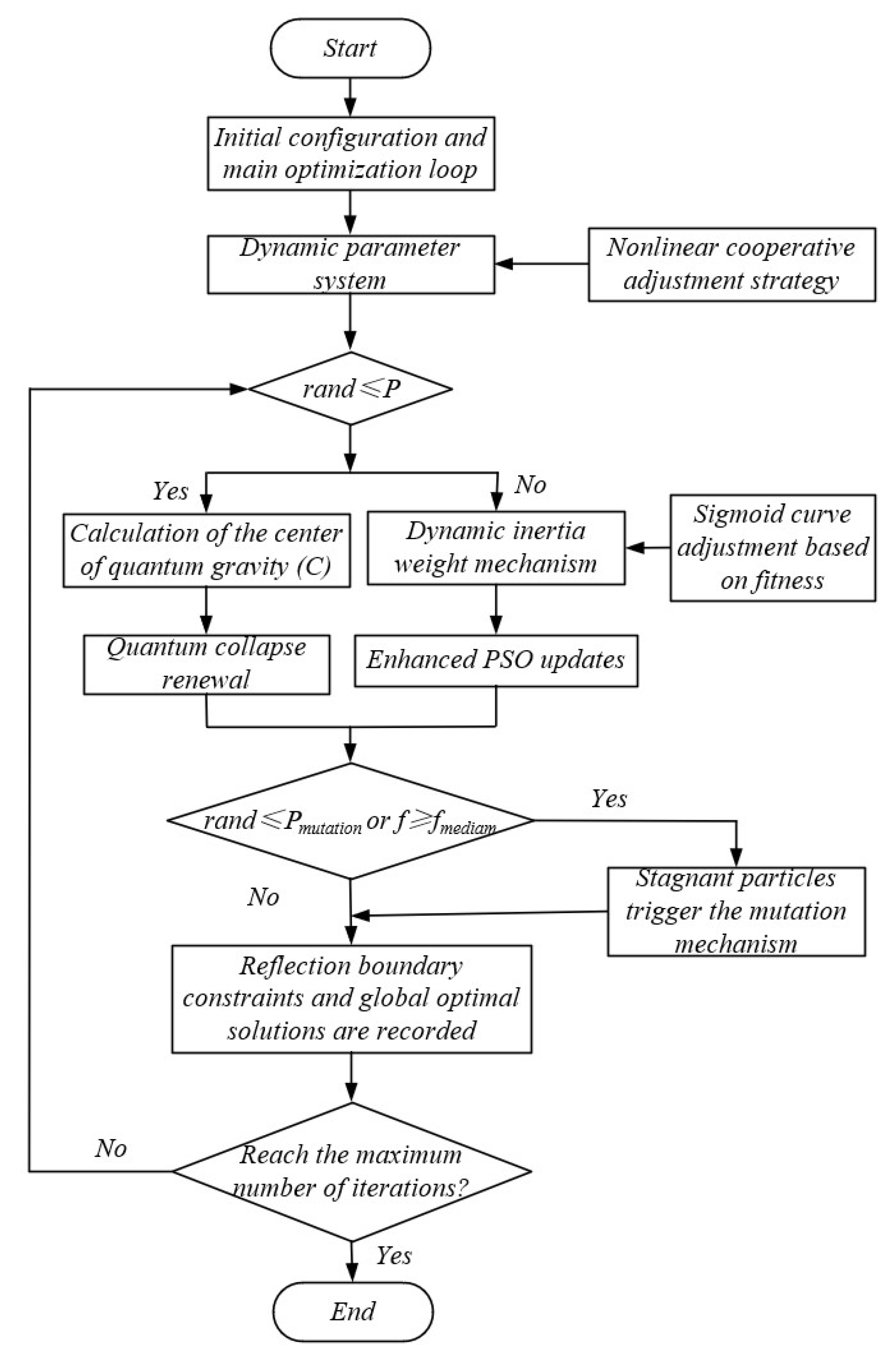
2. Quantum Hybrid Particle Swarm Optimization Algorithm Combined with Quantum Behavior

2.1. Classical Particle Swarm Optimization Algorithm

As a swarm intelligence optimization algorithm, the classical particle swarm optimization (PSO) algorithm, by virtue of information-sharing and collaborative cooperation among individuals within the swarm, is capable of providing the optimal solutions of single-variable or multi-variable problems and has demonstrated unique advantages in a wide range of optimization fields. Within the framework of the PSO algorithm, p b e s t i is defined as the individual optimal position of the i-th particle up to the t-th iteration, while g b e s t represents the current global optimal position of the entire swarm. The update of particle velocity and position follows Equations (1) and (2):
ν i ( t + 1 ) = W ν i ( t ) + c 1 r a n d ( p b e s t i x i ( t ) ) + c 2 r a n d ( g b e s t x i ( t ) )
x i ( t + 1 ) = x i ( t ) + ν i ( t + 1 )
where ν i ( t ) and x i ( t ) denote the velocity and position of the i-th particle at the t-th iteration, respectively; W denotes the inertia weight, which represents the proportion of the velocity inherited from the previous iteration; c 1 and c 2 are the learning factors that control the learning degree of the particle’s optimal position and velocity; r a n d is a random number where r a n d 0 , 1 .
In PSO, parameter settings, especially inertia weight and learning factors, significantly affect iterative performance. Improper inertia weight settings can cause the optimization to converge to local optima prematurely. To address this, a nonlinear inertia weight calculation strategy is proposed [19]:
W = W min + ( W max - W min ) 1 + e 5 × f n o r m a l i z e d - 0.5
Here, W max = 0.9 and W min = 0.4 . The definition of w incorporates an enhanced sigmoid function in the denominator to boost the algorithm’s early exploration and late exploitation capabilities [20]. f n o r m a l i z e d is defined as:
f n o r m a l i z e d = f f min f max f min + e p s
Among them, f is the current particle fitness value, f min and f max are the minimum and maximum values of the group fitness, respectively, and a minimum point e p s is added among them to prevent division by zero errors.
In the classical particle swarm optimization (PSO) algorithm, the cognitive learning factor c 1 and the social learning factor c 2 are typically set as fixed parameters. However, in high-dimensional nonlinear optimization problems such as sparse linear array pattern synthesis, the fixed parameter strategy is prone to causing the algorithm to fall into local optima, significantly weakening its global exploration ability. To address this issue, this paper proposes a dynamic adaptive learning factor adjustment mechanism. Compared with the traditional fixed parameter method, this strategy can dynamically adjust the balance between local exploitation and global exploration according to the population evolution state in real time, thereby enhancing the exploration ability in the early iteration to avoid premature convergence and strengthening the exploitation ability in the later stage to improve the convergence accuracy. Theoretical analysis and experimental results indicate that this dynamic adjustment strategy not only significantly enhances the algorithm’s ability to escape local maxima but also demonstrates superior performance in terms of convergence speed and optimization accuracy, providing a new idea for complex array pattern optimization problems.
c 1 = 2.8 × 1 t T 2 × W c 2 = cos 1 t T × π 2 + 3
In the above two equations, t represents the current iteration number, and T represents the total number of iterations. In the definition of c 1 , the inertia weight W is introduced. By coupling W and c 1 , its initial value is larger (strong exploration ability), and it decreases later (strong exploitation ability) [21]. The dynamic coupling strategy between the individual learning factor c 1 and the inertia weight W is the key innovation used to enhance the algorithm’s global search ability, especially in complex high-dimensional problems such as sparse array optimization, reducing the dependence on the historical optimal position and enhancing the local search ability. For c 2 , the balance between the particle’s global exploration and local exploitation ability is adjusted in real time through a cosine function [20].

2.2. Quantum-Behaved Optimization Algorithm

The quantum-behaved optimization (QBA) algorithm mimics the movement of quantum particles in a potential field towards the lowest energy state. It analogizes the optimization search space to a quantum potential well, where the global optimum corresponds to the lowest potential energy point. Unlike the inertia-weight-driven convergence of PSO, the QBA approaches the optimum by leveraging quantum gate operations and tunneling effects. Its key advantage lies in the quantum probability distribution mechanism, which significantly enhances global exploration and effectively avoids premature convergence, addressing the local optimum trap issue of classical PSO. In the QBA, particle positions are updated based on the quantum potential well model and a Monte Carlo strategy, using the following formula [22]:
X i t + 1 = p i + β · M b e s t X i t · ln 1 u
Here, β is the expansion-compression factor, u is a uniformly distributed random number, and u 0 , 1 . The individual particle mean M b e s t and the weighted average of individual and global optima p i are defined as follows [23]:
M b e s t = 1 N i = 1 N p b e s t i p i = φ · p b e s t i + 1 φ · g b e s t i
This step, a core feature of quantum behavior, ensures that the search focuses on high-quality solution regions. Here, p b e s t i is the individual’s historical optimum. The quantum population optimum g b e s t i is also defined using a random number r a n d 0 , 1 .

2.3. Quantum-Behaved Particle Swarm Optimization Algorithm

The quantum-behaved particle swarm optimization (QPSO) algorithm integrates PSO optimization mechanisms with quantum-inspired strategies. It uses parallel fitness evaluation to compute the objective function for all individuals in the population. Its core process is shown in Figure 1.
In QPSO, the PSO update dominates in the early iterations, leveraging its velocity term advantage to rapidly approach the global optimum. As iterations progress, the probability of quantum collapse update gradually increases, fully utilizing the local fine search capability of quantum behavior to compensate for the PSO’s tendency to fall into local optima. The relevant definitions are as follows:
X t = C + β C X t 1 ln 1 u r a n d p X t 1 + a l p h a c 1 r a n d ( p b e s t i x i ( t ) ) + c 2 r a n d ( g b e s t x i ( t ) ) + m r a n d p
The real-time optimal position of particles is calculated using a hybrid strategy probability mechanism, which involves both quantum collapse and PSO−dominated position updates. Here, r a n d 0 , 1 and the critical probability p are introduced, defined as:
p = 0.2 + 0.6 1 e 5 t T
p is a dynamically adjusted value that invokes a power function to control the update method that is suitable for the current particles, based on the iteration count.
When r a n d p , the quantum behavior of a particle update is triggered. In this case, the gravitational center C of quantum behavior replaces the real-time global optimum g b e s t of PSO, defined as:
C = s u m p b e s t 1 / p b e s t f i t n e s s + e p s , 1 / s u m 1 / p b e s t f i t n e s s + e p s
By introducing an inverse fitness weighting mechanism, the numerator is the row vector of the product of particle position and inverse fitness, and the denominator is the sum of C , namely, the inverse fitness of the population. This design effectively avoids the risk of division by zero, enhances the numerical calculation stability, and uses the quantum gravitational effect to guide particles to accurately search for high-quality solution regions.
The improved quantum behavior replaces the original g b e s t with the gravitational center C and introduces a contraction factor β to further enhance local search efficiency. Its value is defined as:
β = 0.3 1 + sin π t / T
When r a n d p , the position update mechanism that is dominated by the particle swarm algorithm is triggered. Its definition is different from the calculation method shown in Equation (3). In addition to using the improved sigmoid-type inertia weight W as the variable factor of c 1 in Equation (5), the classic inertia weight in the particle swarm algorithm is also replaced by the momentum term [24]. It is defined as:
m = 0.3 X t 1 X a v e r a g e
In the above equation, X t 1 and X a v e r a g e represent the position of the particle in the previous iteration and the average of the previous positions, respectively. Moreover, the gravitational coefficient a l p h a is newly added in its definition:
a l p h a = 1.2 1 t / T 2
This represents the step length of particle movement in each position update.
Compared with the classic particle swarm algorithm, QPSO also introduces the mutation operation in genetic algorithms, which is specifically defined as:
σ = 0.1 + 0.4 1 t / T r a n d P m u t a t i o n f i f m e d i a m
The mutation intensity σ is dynamically adjusted and decreases with the increase in iteration times. The triggering condition is that the fitness value of the particle is greater than the fitness value of the entire population, or the uniform random number is less than the basic variable. The P m u t a t i o n is defined as:
P m u t a t i o n = 0.2 1 tanh 4 t / T
For the selected particles to be mutated, Gaussian perturbation is performed to prevent high-fitness particles from falling into local optima, and the latest particle position is obtained as follows:
X t n e w = X t - 1 o i d + s × d max - d min × r a n d X t f i n a l = min max X t n e w , d min , d max
The position of the particle is subjected to boundary constraints to ensure that it is within the constrained range. The boundary range is also redefined as:
X t = 2 d m a x - X t                       X t > d m a x 2 d m i n - X t                       X t < d m i n                 X t                                 e l s e
The particle position is truncated to X t = min max X t , d max to ensure that the search process always focuses on the effective solution space and avoids interference from out-of-bound solutions in the optimization process.
The pseudo-code of the bat algorithm is shown in Algorithm 1:
Algorithm 1 Quantum-behaved Particle Swarm Optimization Algorithm
Input:
Population size M, maximum generations T , search space constraints: d max , d min , Initial parameters: W max , W min , α 0 , β 0 , p m 0
Output:
the optimal result
Initialization
Initialize population: P = d i 1 M , d i U d min , d max N 1
Initialize personal bests p b e s t p , for t = 1 to T do and r a n d 0 , 1 , g b e s t P S L L min
If ( r a n d satisfies the first item in Equation (9)) then
The quantum gravitational center is calculated by Equation (8), and then by Equations (6), (7), (11) to (13)
The update of its particle positions mainly relies on the first term of Equation (9)
Else
Update the inertia weight and learning factor through (3) to (5)
The update of the positions of its particle swarm relies on the second term in Equation (9)
If ( r a n d satisfies Equation (14)) then
The stop particle triggers the mutation operation through Equation (14)
The updated particle positions and boundaries are shown in Equations (15) and (16)
else
Retain the population positions
end if
Select the best individuals in the population and retain them for the next generation
end for
return Outputs

3. Experiments and Analyses

To verify the optimization performance of the proposed algorithm in sparse antenna arrays, this study conducted numerical simulation experiments on three typical array structures, namely, sparse linear arrays, planar arrays, and concentric circular arrays. In the comparative experiments, the classical particle swarm optimization (PSO), grey wolf optimization (GWO), and whale optimization algorithm (WOA) were selected as benchmark algorithms. The parameters of the comparative algorithms were all set according to authoritative references: the parameters of the PSO algorithm were set according to Reference [25], the modulation parameters of the WOA algorithm were determined according to Reference [26], and the parameters of the GWO algorithm were adopted from the recommended values in Reference [27].
To ensure the reliability of the experimental results and to fully demonstrate the superior performance of the proposed algorithm in terms of sidelobe level suppression, unified test conditions were used in the experiments: the population size was set to 50 individuals, and the maximum number of iterations was limited to 300 generations. Considering the stochastic nature of optimization algorithms, each algorithm was independently run five times, and the optimal results were selected for comparative analysis. This experimental design not only ensures statistical significance but also objectively reflects the differences in the optimal solution search capabilities of the various algorithms.

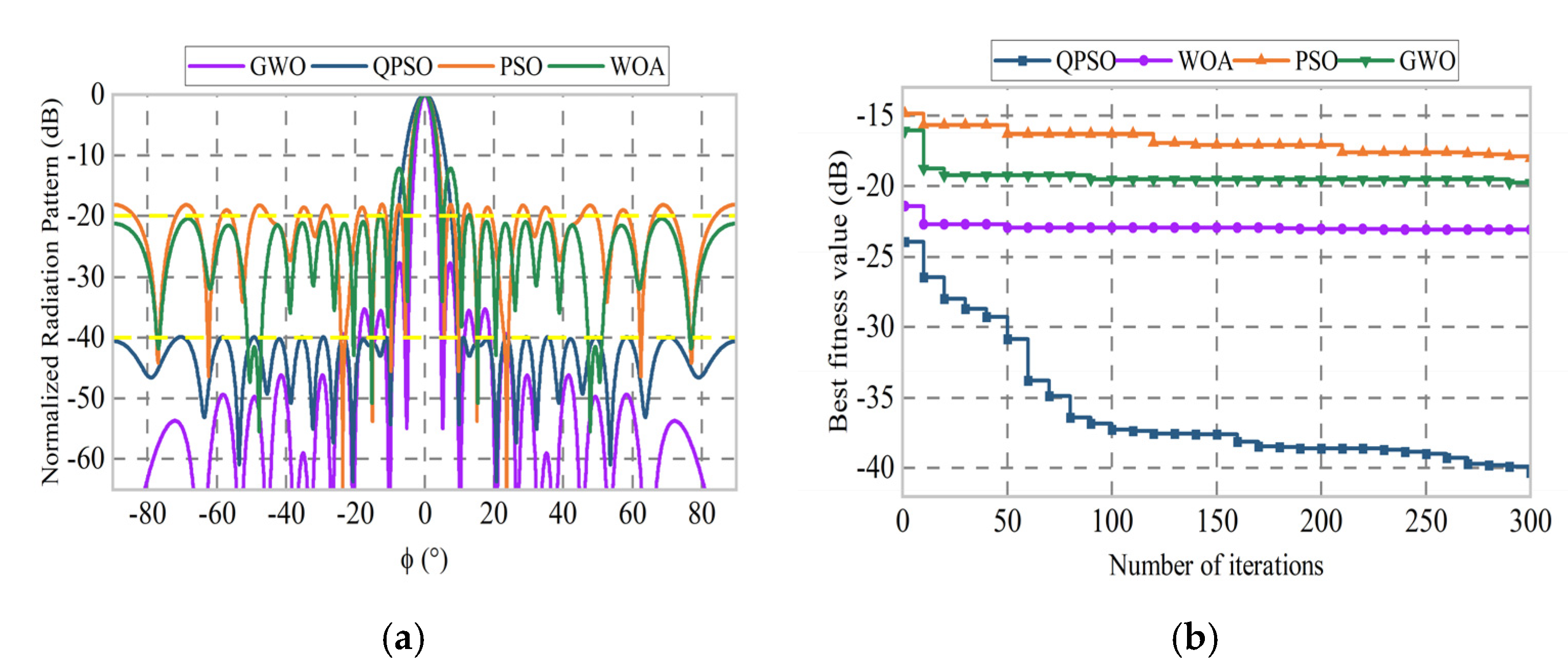
3.1. Sparse Linear Array Simulation Test

Sparse arrays, known for their simple structure and easy implementation, are widely used in engineering applications. Taking linear arrays as an example, common sparse arrays usually contain an odd number of array elements, positioned symmetrically around the central unit within a fixed aperture.
For arrays with fixed excitation amplitude and varying phases, the array factor is expressed as follows:
A F ( θ ) = n = 0 N 1 I n e j ( n k d s i n ( θ ) + ϕ n )
where the default excitation amplitude of each array element is assumed to be I n ; d is the spacing between adjacent antenna elements, θ is the incident beam angle, ϕ n is the phase deviation of the nth antenna, k is the wavenumber, defined as k = 2 π / λ where λ is the wavelength, and θ is the observation angle. Figure 2 is a schematic diagram of a common linear array:
This paper presents an innovative antenna array design, employing a series-fed approach [28]. The spacing between every two antenna elements varies, eliminating the need for an overall symmetrical layout while achieving low sidelobe performance. The relevant schematic is shown in Figure 3.
The entire antenna array is fed by a single source. Multiple one-to-two power dividers facilitate hierarchical feeding. One branch passes through amplitude and phase compensators to ensure consistent excitation and random phase compensation. The other branch feeds subsequent elements via a feedline running through the entire radiating cavity, enabling convenient feeding.
The optimization models for element positions and phases are defined as follows:
d min = d c = 0.5 λ d i d max = λ i = 1 N d i = L min ( P S L L ( d 1 , d 2 , , d n ) )
where PSLL (peak sidelobe level) is defined as the maximum radiation intensity in the sidelobe region of the array radiation pattern. Its mathematical expression is:
P S L L = 20 log 10 max A F θ / A F θ 0
To compare algorithm performance, all optimization models were implemented on the MATLAB 2021(b) simulation platform under uniform conditions of equal amplitude excitation ( I n = 1) and fixed aperture size (D = 10.43 λ ). Figure 4a presents the comparison results of normalized radiation patterns, and Figure 4b shows the PSLL convergence curves of the algorithms.
As shown in Figure 4, the quantum-behaved particle swarm optimization (QPSO) algorithm proposed in this paper is compared with three typical optimization algorithms: classic particle swarm optimization (PSO), the grey wolf optimizer (GWO), and the whale optimization algorithm (WOA). Figure 4a indicates that the QPSO algorithm achieves the best sidelobe suppression performance (PSLL = −20.46 dB), surpassing the WOA (−19.6 dB), the GWO (−18.86 dB), and PSO (−18.15 dB). The convergence analysis in Figure 4b shows that the WOA algorithm exhibits the fastest initial convergence speed, while the QPSO algorithm attains the global optimal solution after 200 iterations. The element spacing distribution optimized by QPSO is presented in Table 1. Its non-uniform characteristics contribute to the aforementioned sidelobe suppression effect.
Table 2 provides a comparison of the proposed algorithm with classical particle swarm optimization (PSO) and the Lévy flight particle swarm optimization (LFPSO) algorithms from other works in the literature.
As shown in Table 2, when the number of array elements is fixed, the quantum-behaved particle swarm optimization (QPSO) algorithm has certain advantages over the LFPSO algorithm in terms of element spacing requirements and the number of iterations. Specifically, the peak sidelobe level (PSLL) of QPSO is −20.46 dB, which is significantly lower than that of LFPSO (−19.61 dB). Moreover, compared with the PSO algorithm in Reference [25], QPSO achieves a lower sidelobe level than the best result (−19.87 dB) reported in that study, even though the number of iterations for QPSO is 100 more than that used in Reference [25].

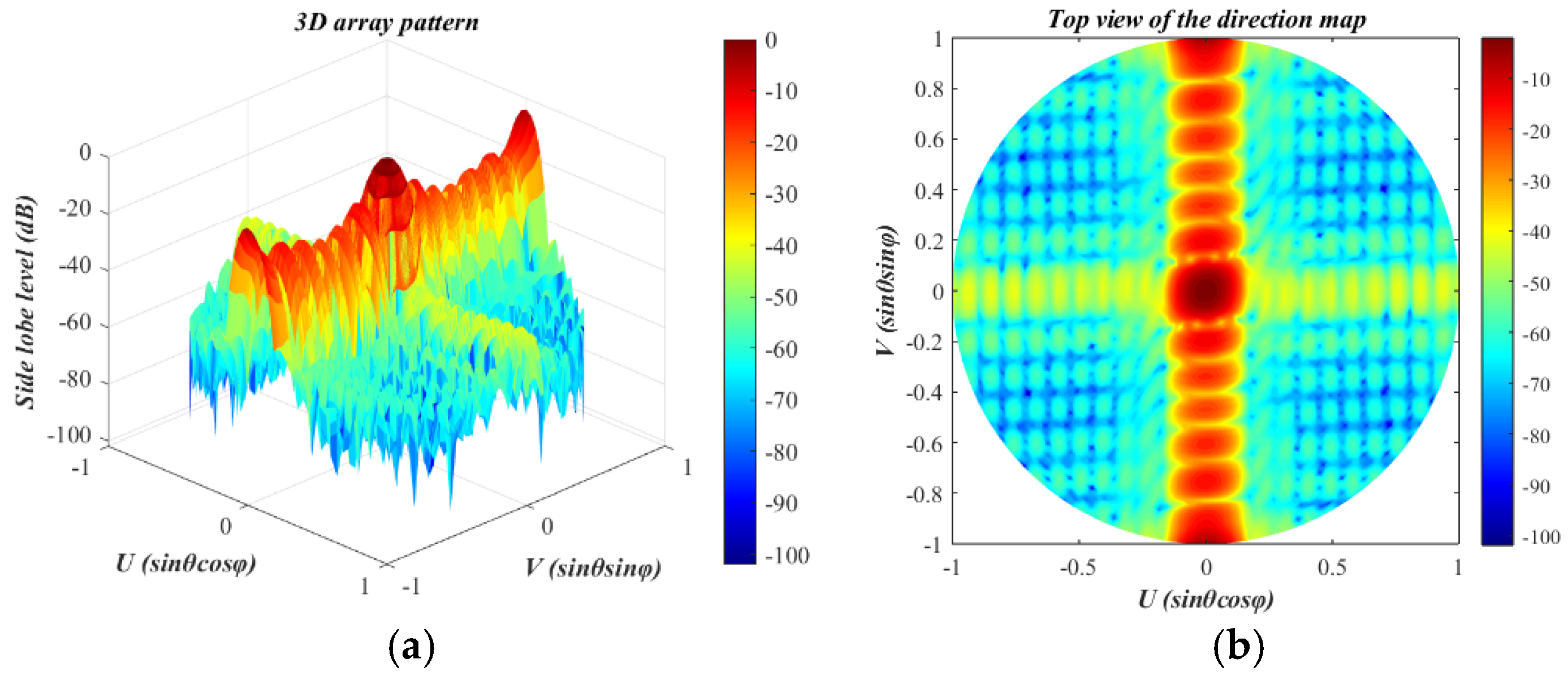
3.2. Sparse Matrix Simulation Test

This study constructs a rectangular sparse array model of M × N with a physical aperture size of L × H . To avoid element-coupling effects, the minimum element spacing is set to d min = 0.5 λ , where λ is the operating wavelength. The main beam is directed at θ 0 , φ 0 . Under equal-amplitude excitation, the array pattern function is:
F θ , φ = m = 1 M n = 1 N e j k x m n sin θ cos φ sin θ 0 cos φ 0 + y m n sin θ sin φ sin θ 0 sin φ 0
Using the first quadrant coordinate system, x m n , y m n represents the two-dimensional coordinates of the m , n -th element in the non-uniform grid, where x m n and y m n denote the horizontal and vertical distances of the i-th element from the origin, respectively, and they satisfy x m n L , Y m n H .
To better search for the positions of the elements, a position optimization matrix is established:
X = x 1 , 1 x 1 , n x m , 1 x m , n ,           Y = y 1 , 1 y 1 , n y m , 1 y m , n          
For the sum of the dimensions of the matrix, we find:
X × Y M × N ,         L x max   X L x min ,         H y max Y H y min
The fitness values of the two matrices are used as a reference for measuring the sidelobe level. To maintain the aperture size, elements are fixed at the four corners of the array:
N 1 x 1 = 0 , y 1 = 0 ; N 2 x 2 = L , y 2 = H N 3 x 3 = 0 , y 3 = L ; N 4 x 4 = H , y 4 = 0
The relevant schematic is shown in Figure 5.
The calculation method for PSLL is as follows:
P S L L = min max ϕ S 1 F θ 0 , φ ; θ 0 , φ 0 max F θ 0 , φ ; θ 0 , φ 0 + max ϕ S 2 F θ 0 , φ ; θ 0 , φ 0 max F θ 0 , φ ; θ 0 , φ 0
In the above formula, the first term represents the sidelobe region of the array pattern at a specific azimuth angle, and the second term represents the sidelobe region in the pitch direction at a specific elevation angle. The overall peak sidelobe level is the sum of the fitness functions of the two. The array synthesis model is as follows:
max P S L L s u m       f i t n e s s X , Y N 1 , N 2 , N 3 , N 4 x min = 0.5 λ x i x max   = λ ,         y min = 0.5 λ y j y max = λ x m n L , Y m n H
The simulation experiments were conducted using the control variable method, and the key parameters of each algorithm were optimized through parameter scanning. The simulation results are as follows.
In Figure 6a, among the normalized array factor patterns of the four algorithms, the sidelobe levels of classical PSO and the GWO are relatively high, exceeding −20 dB, while those of the QPSO and WOA are below −20 dB.
Further analysis shows that in the GWO, except for the first three sidelobes, the others are below −40 dB. Notably, the hybrid optimization algorithm proposed in this paper achieves excellent sidelobe suppression, with all sidelobes below −40 dB. Figure 6b shows that the proposed hybrid optimization algorithm outperforms the other three in terms of global search performance and resistance to local convergence. It successfully escapes local optima in the late iteration stage and converges to the global optimum after 300 iterations, indicating its superior robustness and stability.
Figure 7a presents the 3D pattern of a sparse matrix. The radiation field is distributed across all four quadrants, with maximum radiation θ 0 = 0 , φ 0 = 0 at the origin. At a specific angle, the sidelobe radiation intensity where φ = 90 is more significant than in other directions, when φ = 0 .
This radiation characteristic is crucial for antenna array pattern optimization as it directly impacts the antenna’s radiation performance and sidelobe levels in different directions.
To more intuitively illustrate the comparative performance of QPSO in the radiation pattern of sparse arrays, the results are summarized in Table 3, along with several other sparse planar rectangular array optimization algorithms.
Among these three algorithms, the PSLL values are all taken as the minimum values from the elevation and azimuth planes. Compared with the arithmetic optimization algorithm (AOA), the QPSO achieves a significantly lower sidelobe level of −40.26 dB under stricter aperture requirements and a smaller number of iterations, which is a much lower level than the −34.78 dB obtained by the AOA. When the number of iterations is the same, QPSO demonstrates a lower PSLL than the chaotic global algorithm (CGA) under more stringent array aperture and element spacing conditions, with a PSLL of −40.26 dB compared to −34.36 dB with the CGA.

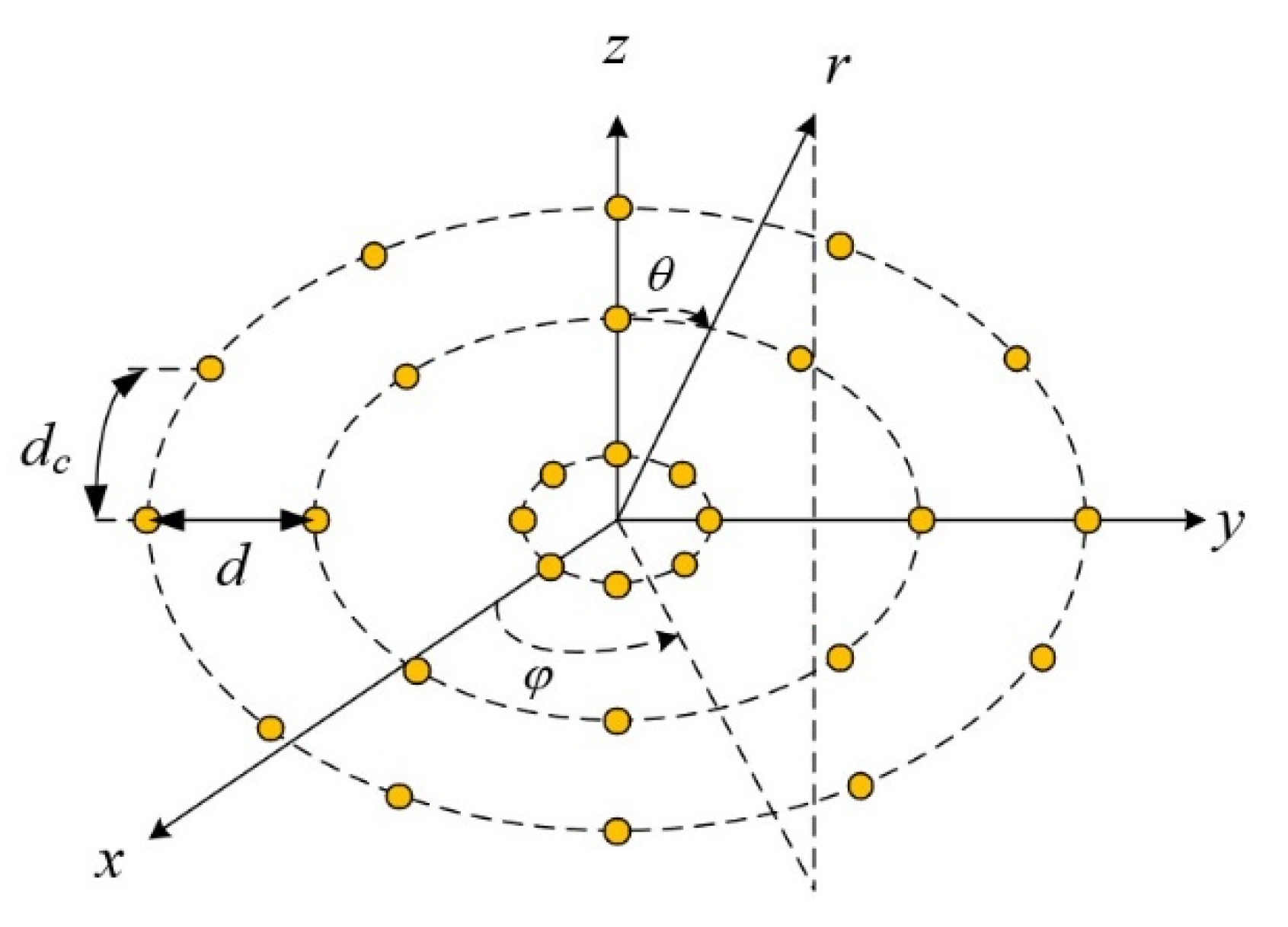
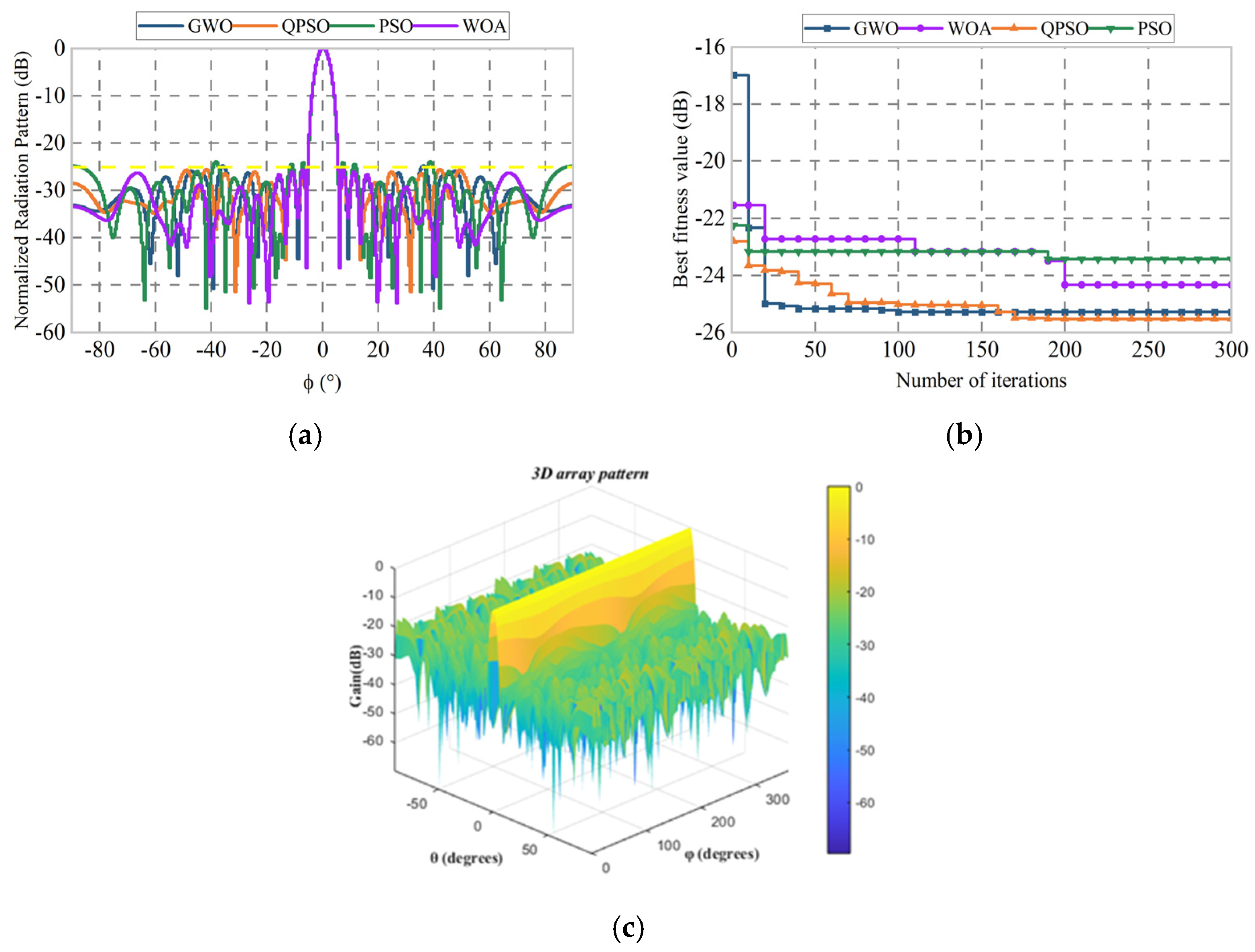
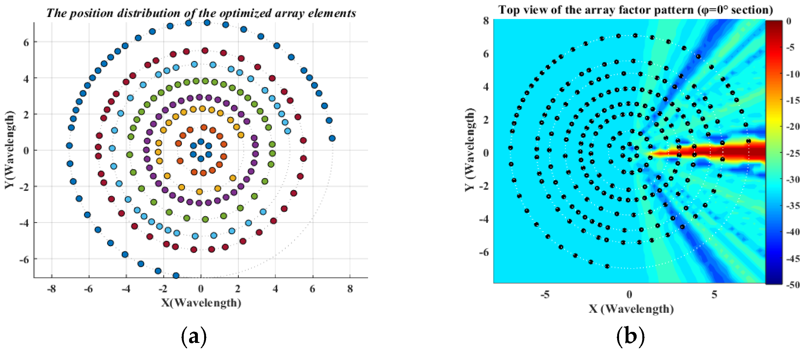
3.3. Sparse Multi-Ring Concentric Circular Array

This study proposes a sparse concentric circular array. Due to the identical center position in concentric circular arrays, it can be regarded as the combination of multiple uniform concentric circular arrays, and a classic array is shown in Figure 8.
By substituting the coordinates of the elements in a uniform concentric circular array with polar coordinates, we have:
x = R cos φ y = R sin φ R 2 = x 2 + y 2 k u = ξ cos ψ k ν = ξ sin ψ ξ 2 = k u 2 + k v 2
For a concentric circular array with M rings and N m elements on the m -th ring, the array factor in polar coordinates can be written as:
F ξ , ψ = m = 0 M N m I R m , φ n p = + J N m p + k R m ξ e j N m p + k ψ
where J N m p + k R m ξ denotes the zeroth-order Bessel function, defined as:
J n x = 1 2 π π π e j x sin θ n θ d θ = 1 π 0 π cos x sin θ n θ d θ
Based on the Fourier relationship between the excitation of the antenna circular array elements and the pattern, a Fourier–Bessel transform exists between them. Using this time-frequency conversion, the position problem of concentric circular array elements can be transformed into an excitation energy problem involving array antennas. By considering the three optimization objectives of sparse interleaved arrays—the approximate uniformity of subarray patterns, the low sidelobe levels of individual subarray patterns, and the interleaved distribution of each antenna element—the optimal mathematical model is established as follows:
s u b a r r a y i min P S L p 1 , p 2 , , p N = max F u i F F i max s u b a r r a y i min P S L p 1 , p 2 , , p N = max F u i F F j max s .   t . min Δ = P S L L i P S L L j W i d t h s u b a r r a y i = W i d t h s u b a r r a y j n 1 , N , m 1 , M , p m q n
In the above formula, F u i is the value of the sidelobe region of the subarray, and F F i max is the gain value of the main lobe of the pattern of the i -th subarray. W i d t h s u b a r r a y i is the width of the main lobe in subarray direction i , while p m and p n represent the positions of the subarray elements.
A new element position optimization model is established to ensure sparse arrangement:
d i min = 0.5 λ d c d i max = 0.8 λ d min = 0.5 λ d d max = 0.8 λ N min = 6 N n N m N max = 40                             n m    
Here, d c is the spacing between elements in the same ring, randomly distributed between 0.5 and 0.8 λ ; d represents the spacing between different rings; and N is the number of elements on each ring, which increases gradually with the increase in the ring spacing.
In simulation tests, the particle number is set to 50, and the iteration number to 300. The number of concentric circular rings is set to 8, and the number of elements increases nonlinearly from 6 to 40. The above optimization model is incorporated into four algorithms, and the array factor patterns and sidelobe level iteration curves are obtained as shown in Figure 9.
During the sidelobe level iteration of the four algorithms, the maximum sidelobe levels of all algorithms are below −20 dB, but only the grey wolf optimizer and quantum-behaved particle swarm optimization algorithms achieve a value below −25 dB. As shown in Figure 9b, the proposed hybrid optimization algorithm shows superior search ability and stability compared to the grey wolf optimizer in the late iteration stage.
Figure 10a shows the element position layout of the array. The array, centered at the origin, has its elements distributed sparsely across 8 rings. The radiation pattern of the array is shown when φ = 0 in Figure 10b.
Table 4 presents the comparison results between the QPSO algorithm and the iterative convex optimization (ICO) and the improved differential evolution algorithm (DEA):
In the two references for the DEA and ICO, the maximum radius of the array is approximate, and the PSLL values of −24.67 dB and −24.10 dB are quite close. In contrast, QPSO achieves a significantly lower PSLL of −25.53 dB, with a number of array elements comparable to those of ICO.
It is worth noting that References [33,34] primarily focus on optimizing a single variable, whereas the current work optimizes multiple variables, including element spacing, the number of elements, and the aperture between concentric rings. This comprehensive optimization approach provides a meaningful basis for comparison.

4. Conclusions

This study proposes a novel hybrid optimization algorithm (QPSO). Through the synergistic effect of the quantum potential well model and the adaptive genetic variation mechanism, it effectively solves the multi-peak optimization problem found in the pattern synthesis of sparse array antennas. This algorithm shows significant advantages in the optimization of linear arrays (PSLL = −20.45 dB), planar rectangular arrays (full sidelobes < −40 dB), and multi-ring concentric circular arrays (PSLL = −25.53 dB), and represents a considerable improvement compared with the traditional PSO, GWO, and WOA algorithms. Its innovation is reflected in: (1) the quantum tunneling effect, which enhances global exploration ability; (2) dynamic mutation probability, which maintains population diversity; (3) the elitist retention strategy, which ensures convergence stability. These characteristics provide new solutions for the optimization of large-scale array antennas.

Author Contributions

Conceptualization, Y.L. and L.H.; methodology, Y.L., L.H. and X.X.; validation, X.X.; writing—original draft preparation, Y.L. and L.H.; writing—review and editing, Y.L. and H.Y. All authors have read and agreed to the published version of the manuscript.

Funding

This work was supported by the Hubei Provincial Natural Science Foundation of China, 2024AFB966.

Institutional Review Board Statement

Not applicable.

Informed Consent Statement

Not applicable.

Data Availability Statement

The original contributions presented in this study are included in the article. Further inquiries can be directed to the corresponding author and the first author.

Acknowledgments

We thank the editor and the anonymous reviewers for their constructive comments, which helped to improve our work.

Conflicts of Interest

The authors declare no conflicts of interest.

Abbreviations

The following abbreviations are used in this manuscript:
QPSOQuantum-behaved particle swarm optimization algorithm
WOAWhale optimization algorithm
LFPSOLevi’s flying particle swarm optimization
PSLLPeak sidelobe level
GWOGrey wolf optimization algorithm
AOAArithmetic optimization algorithm
CGAChaotic genetic algorithm
DEADifferential evolution algorithm
ICOIterative convex optimization algorithm

References

  1. Ma, W.; Zhu, L.; Zhang, R. Multi-beam forming with movable-antenna array. IEEE Commun. Lett. 2024, 28, 697–701. [Google Scholar] [CrossRef]
  2. Saeed, M.A.; Nwajana, A.O. A review of beamforming microstrip patch antenna array for future 5G/6G networks. Front. Mech. Eng. 2024, 9, 1288171. [Google Scholar] [CrossRef]
  3. Geyi, W. The method of maximum power transmission efficiency for the design of antenna arrays. IEEE Open J. Antennas Propag. 2021, 2, 412–430. [Google Scholar] [CrossRef]
  4. Zhang, L.; Marcus, C.; Lin, D.; Mejorado, D.; Schoen, S.J.; Pierce, T.T.; Kumar, V.; Fernandez, S.V.; Hunt, D.; Li, Q.; et al. A conformable phased-array ultrasound patch for bladder volume monitoring. Nat. Electron. 2024, 7, 77–90. [Google Scholar] [CrossRef]
  5. Ji, L.; Ren, Z.; Chen, Y.; Zeng, H. Large-Scale Sparse Antenna Array Optimization for RCS Reduction with an AM-FCSN. IEEE Sens. J. 2024, 25, 5782–5794. [Google Scholar] [CrossRef]
  6. Owoola, E.O.; Xia, K.; Wang, T.; Umar, A.; Akindele, R.G. Pattern synthesis of uniform and sparse linear antenna array using mayfly algorithm. IEEE Access 2021, 9, 77954–77975. [Google Scholar] [CrossRef]
  7. Wu, P.; Liu, Y.-H.; Zhao, Z.-Q.; Liu, Q.-H. Sparse antenna array design methodologies—A review. J. Electron. Sci. Technol. 2024, 22, 100276. [Google Scholar] [CrossRef]
  8. Shao, W.; Hu, J.; Ji, Y.; Zhang, W.; Fang, G. W-Band FMCW MIMO System for 3-D Imaging Based on Sparse Array. Electronics 2024, 13, 369. [Google Scholar] [CrossRef]
  9. Chen, D.; Schlegel, A.; Nanzer, J.A. Imageless contraband detection using a millimeter-wave dynamic antenna array via spatial fourier domain sampling. IEEE Access 2024, 12, 149543–149556. [Google Scholar] [CrossRef]
  10. Yangyu, X.; Weimin, J.; Fenggan, Z. Pattern optimization of thinned linear arrays based on improved cuckoo search algorithm. Mod. Electron. Tech. 2021, 44, 7–12. [Google Scholar]
  11. Xue, T.; Bin, W.; Jingrui, L. A synthesis method for thinned linear arrays based on improved sparrow search algorithm. J. Microw. 2022, 38, 43–51. [Google Scholar]
  12. Zhang, S.R.; Zhang, Y.X.; Cui, C.Y. Efficient multiobjective optimization of time-modulated array using a hybrid particle swarm algorithm with convex programming. IEEE Antennas Wirel. Propag. Lett. 2020, 19, 1842–1846. [Google Scholar] [CrossRef]
  13. Tinh, N.D. Optimization of Radiation Pattern for Circular Antenna Array using Genetic Algorithm and Particle Swarm Optimization with Combined Objective Function. IEIE Trans. Smart Process. Comput. 2024, 13, 579–586. [Google Scholar]
  14. Zang, Z.; Wu, J.; Huang, Q. Design of an Aperiodic Optical Phased Array Based on the Multi-Strategy Enhanced Particle Swarm Optimization Algorithm. Photonics 2025, 12, 210. [Google Scholar] [CrossRef]
  15. Zhu, T.; Liu, Y.; Li, J.; Zhao, W. Optimization of time modulated array antennas based on improved gray wolf optimizer. AIP Adv. 2025, 15, 025126. [Google Scholar] [CrossRef]
  16. Bouchachi, I.; Reddaf, A.; Boudjerda, M.; Alhassoon, K.; Babes, B.; Alsunaydih, F.N.; Ali, E.; Alsharef, M.; Alsaleem, F. Design and performances improvement of an UWB antenna with DGS structure using a grey wolf optimization algorithm. Heliyon 2024, 10, e26337. [Google Scholar] [CrossRef] [PubMed]
  17. Amiriebrahimabadi, M.; Mansouri, N. A comprehensive survey of feature selection techniques based on whale optimization algorithm. Multimed. Tools Appl. 2024, 83, 47775–47846. [Google Scholar] [CrossRef]
  18. Liu, L.; Zhang, R. Multistrategy improved whale optimization algorithm and its application. Comput. Intell. Neurosci. 2022, 2022, 3418269. [Google Scholar] [CrossRef] [PubMed]
  19. Xu, C. Application of Improved Particle Swarm Optimization in Array Antenna Beamforming. Master’s Thesis, Nanjing University of Posts and Telecommunications, Nanjing, China, 2022. [Google Scholar] [CrossRef]
  20. Zhang, T.Y. Research on Sparse Array Optimization Based on Intelligent Optimization Algorithms. Ph.D. Thesis, Shijiazhuang Tiedao University, Shijiazhuang, China, 2024. [Google Scholar] [CrossRef]
  21. Zhao, Y.D.; Fang, Z.H. Particle swarm optimization algorithm with weight function learning factors. J. Comput. Appl. 2013, 33, 2265–2268. [Google Scholar]
  22. Yang, C.X.; Zhang, J.; Tong, M.S. A hybrid quantum-behaved particle swarm optimization algorithm for solving inverse scattering problems. IEEE Trans. Antennas Propag. 2021, 69, 5861–5869. [Google Scholar] [CrossRef]
  23. Fahad, S.; Yang, S.; Khan, S.U.; Khan, S.A.; Khan, R.A. A hybrid smart quantum particle swarm optimization for multimodal electromagnetic design problems. IEEE Access 2022, 10, 72339–72347. [Google Scholar] [CrossRef]
  24. Xue, W. An Improved Particle Swarm Optimization Algorithm with Inertia Weight. Mod. Inf. Technol. 2023, 7, 88–91. [Google Scholar] [CrossRef]
  25. Zheng, S.; Zhao, X.; Zhang, C.; Li, Y.; Chai, M. Multi-objective optimization of hydraulic performance for low-specific-speed stamping centrifugal pump based on PSO algorithm. Trans. Chin. Soc. Agric. Mach. 2025, 56, 353–360. [Google Scholar]
  26. Zhao, Z.H.; Yin, Y.F.; Wang, Y.K.; Qin, K.R.; Xue, C.D. Adaptive ECG Signal Denoising Algorithm Based on the Improved Whale Optimization Algorithm. IEEE Sens. J. 2024, 24, 34788–34797. [Google Scholar] [CrossRef]
  27. He, J.; Hong, Z.; Sun, X.; Deng, Q.; Zhu, M.; Zhu, C.; Liu, K.; Sun, B.; Yao, J. Three-dimensional Image Reconstruction of Breast Tumor by Electrical Impedance Tomography based on Dimensional Grey Wolf Optimization Algorithm. IEEE Trans. Instrum. Meas. 2025, 74, 4504310. [Google Scholar] [CrossRef]
  28. Liu, Y.; Huang, L.; Li, H.; Sun, C. Dual-Frequency Common-Cable Waveguide Slot Satellite Communication Antenna. Electronics 2025, 14, 1326. [Google Scholar] [CrossRef]
  29. Liu, J.L.; Wang, X.M. Synthesis of sparse arrays with spacing constraints using an improved particle swarm optimization algorithm. J. Microw. 2010, 26, 7–10. [Google Scholar] [CrossRef]
  30. Meng, X.M.; Cai, C.C. Synthesis of sparse array antennas based on Lévy flight particle swarm optimization. J. Terahertz Sci. Electron. Inf. Technol. 2021, 19, 90–95. [Google Scholar]
  31. Qiang, G.; Ye, L.C.; Ni, W.Y.; Wang, Y.; Chernogor, L. Synthesis of sparse planar arrays using an improved arithmetic optimization algorithm. J. Xidian Univ. 2023, 50, 202–212. [Google Scholar] [CrossRef]
  32. Jiang, W.Q.; Zhang, H.M.; Wang, X.F. Research on two-dimensional planar array based on chaotic genetic algorithm. Appl. Electron. Tech. 2023, 49, 68–72. [Google Scholar] [CrossRef]
  33. Cheng, D.D.; Li, Y.M.; Wei, J.; Zhang, F. Optimal design of sparse concentric ring arrays. Syst. Eng. Electron. 2018, 40, 739–745. [Google Scholar]
  34. Aslan, Y.; Roederer, A.; Yarovoy, A. Concentric ring array synthesis for low side lobes: An overview and a tool for optimizing ring radii and angle of rotation. IEEE Access 2021, 9, 120744–120754. [Google Scholar] [CrossRef]
Figure 1. Flowchart of the algorithm.
Applsci 15 06490 g001
Figure 2. Diagram illustrating a common antenna array.
Applsci 15 06490 g002
Figure 3. Schematic diagram of the string feed array transmission system.
Applsci 15 06490 g003
Figure 4. (a) Sparsely distributed linear array pattern; (b) minimum sidelobe−level iteration number diagram.
Applsci 15 06490 g004
Figure 5. Schematic of a sparse rectangular array.
Applsci 15 06490 g005
Figure 6. (a) Pattern of a sparse rectangular array; (b) convergence of the maximum sidelobe level.
Applsci 15 06490 g006
Figure 7. (a) The 3D pattern of a sparse rectangular array; (b) top view of the pattern.
Applsci 15 06490 g007
Figure 8. Schematic of a sparse multi-ring concentric circular array.
Applsci 15 06490 g008
Figure 9. (a) Normalized pattern of a sparse multi-ring concentric circular array; (b) iteration curve; (c) 3D pattern.
Applsci 15 06490 g009
Figure 10. (a) Element layout of a sparse multi-ring concentric circular array; (b) array radiation pattern at φ = 0 .
Applsci 15 06490 g010
Table 1. Spacing table of each unit in a sparse array.
ElementsUnit Spacing ( λ )ElementsUnit Spacing ( λ )
1-219-100.5000
2-30.759710-110.5000
3-40.759911-120.5670
4-50.513612-130.5683
5-60.500013-140.7792
6-70.500014-150.7821
7-80.506515-160.9157
8-90.500016-170.7761
Table 2. Comparison table of several algorithms.
WorkTypeArray ElementsArray TypeIterationsSpacing RequirementPSLL (dB)
[29]LFPSO17Symmetry500 d 0.5 λ −19.61
[30]PSO100 d 0.5 λ −19.87
This workQPSOAsymmetry300 λ d 0.5 λ −20.46
Table 3. Comparison diagrams of several planar sparse array arrangements.
WorkTypeArray ApertureAperture RequirementIterationsParticle QuantityPSLL
(dB)
[31]AOA 9.5 λ × 4.5 λ d 0.5 λ 1000100−34.78
[32]CGA 24 λ × 24 λ d 0.5 λ 20050−34.36
This workQPSO 10.5 λ × 6.5 λ λ d 0.5 λ 300−40.26
Table 4. Comparison of several concentric circles.
WorkTypeArray ApertureAperture RequirementArray ElementsPSLL
(dB)
[33]DEA 4.98 λ d = 0.5 λ /−24.67
[34]ICO 5 λ d 0.5 λ 224−24.10
This workQPSO 3.5 λ 5.6 λ 0.8 λ d 0.5 λ 230−25.53
Disclaimer/Publisher’s Note: The statements, opinions and data contained in all publications are solely those of the individual author(s) and contributor(s) and not of MDPI and/or the editor(s). MDPI and/or the editor(s) disclaim responsibility for any injury to people or property resulting from any ideas, methods, instructions or products referred to in the content.

