Research on an Intelligent Sedimentary Microfacies Recognition Method Based on Convolutional Neural Networks Within the Sequence Stratigraphy of Well Logging Curve Image Groups

Abstract

Sedimentary facies identification constitutes a cornerstone of reservoir engineering. Traditional facies interpretation methods, reliant on manual log-response parameter analysis, are constrained by interpreter subjectivity, reservoir heterogeneity, and inefficiencies in resolving thin interbedded sequences and concealed fluvial sand bodies—issues marked by high interpretive ambiguity, prolonged cycles, and elevated costs. This study focuses on the Lower Cretaceous Yaojia Formation Member 1 (K2y1) in the satellite oilfield of the Songliao Basin, integrating sequence stratigraphy into a machine learning framework to propose an innovative convolutional neural network (CNN)-based facies recognition method using log-curve image groups by graphically transforming five log curves and establishing a CNN model that correlates log responses with microfacies. Results demonstrate the model’s capability to identify six microfacies types (e.g., subaqueous distributary channels, estuary bars, sheet sands) with 83% accuracy, significantly surpassing conventional log facies analysis. This breakthrough in interpreting complex heterogeneous reservoir lithofacies establishes a novel technical avenue for intelligent exploration of subtle hydrocarbon reservoirs.

1. Introduction

Sedimentary facies identification plays a crucial role in reservoir engineering by enabling precise evaluation of reservoir properties (porosity, permeability) through depositional environment analysis (e.g., fluvial, deltaic systems). This approach delineates the spatial distribution of high-quality reservoirs while revealing heterogeneity and connectivity patterns [1]. Particularly at the microscale, targeting optimal sedimentary microfacies is the core objective of well placement. These microfacies directly govern sand–body connectivity and reservoir properties, providing the most refined basis for “sweet spot” identification. Accurate delineation of favorable microfacies distributions is thus paramount to well performance, making prioritized well deployment within optimal microfacies belts a fundamental strategy for enhancing productivity, mitigating geological risks, and optimizing injection–production schemes to maximize recovery efficiency [2]. Machine learning, by automating the processing of voluminous geological data, enables rapid identification of complex depositional facies and elucidation of implicit patterns, substantially improving prediction accuracy and operational efficiency. This advancement drives the transition toward precision and cost-effective reservoir development [3,4].

Sedimentary microfacies recognition has evolved through successive waves of methodological innovation, transitioning from manual interpretation to data-driven automation. Early approaches emphasized multi-source data integration, exemplified by Yong et al.’s [5] synergistic fusion of core-calibrated data, geologic parameters, and principal component-Bayesian models to quantify depositional environments. Concurrently, artificial intelligence began permeating sedimentology: Bhatt et al. [6] enhanced facies classification accuracy via backpropagation neural networks (BPNNs), while Wei [4] pioneered unsupervised learning through self-organizing maps (SOMs) by coupling geological parameters with trend code encoding. Support vector machines (SVMs) emerged as a robust tool for resolving nonlinear microfacies patterns, complemented by fuzzy logic systems [7] and BPNN-driven parameter mapping frameworks [8,9]. These methods collectively addressed limitations of traditional experience-dependent interpretation but remained constrained by manual feature engineering and linear assumptions.

Recent advances have shifted toward deep learning and hybrid paradigms, leveraging automated feature extraction and cross-domain knowledge integration. Convolutional neural networks (CNNs) revolutionized lithofacies classification by transforming 1D log curves into 2D semantic images [10,11], while SVM-enhanced hybrid models achieved 70% accuracy in uncored intervals [11]. Unsupervised techniques like SOM enabled latent pattern discovery through topological clustering [4,9], and multimodal frameworks integrated mathematical models with expert knowledge [12]. The integration of 1D CNNs for temporal data modeling [13] and generative adversarial networks (GANs) for synthetic log generation further expanded methodological diversity [14]. These developments underscore a paradigm shift: modern microfacies analysis prioritizes end-to-end learning architectures that transcend manual feature selection, enabling real-time, basin-scale reservoir characterization with unprecedented precision [15].

This study focuses on the target interval (55–71 m) within the Putaohua oil layer of the Weixing area. Of the 235 wells in the study area, 131 wells were selected based on stringent criteria including data integrity, completeness, and comprehensive logging suites required for robust analysis. Among these qualified wells, two cored wells provide critical lithological and sedimentological constraints, significantly enhancing the fidelity of sedimentary microfacies identification. We utilized natural gamma ray logging (GR), spontaneous potential logging (SP), acoustic logging (AC), lateral deep resistivity logging (LLD), and lateral shallow resistivity logging (LLS), obtaining a total of 2390 valid logging records. Additionally, we designed a multimodal convolutional neural network that jointly inputs dynamic scale imaging slices with the sequence stratigraphic domain conditions represented by one-hot encoding. Through multiple layers of Conv2D and MaxPooling2D operations, the network extracts key features such as sand body boundaries, bedding structures, and sedimentary architectures from the well logging images. These features are then concatenated with the geological significance encoding of the stratigraphic sequence to enhance the model’s understanding of the sedimentary facies control relationships under different stratigraphic sequences, thereby achieving precise classification of sedimentary facies. The application of this multimodal convolutional neural network not only enables accurate classification of sedimentary facies but also provides crucial geological information support for reservoir engineering. This aids in optimizing oil and gas reservoir development strategies and enhancing recovery rates, thereby promoting the efficient utilization and sustainable development of oil and gas resources.

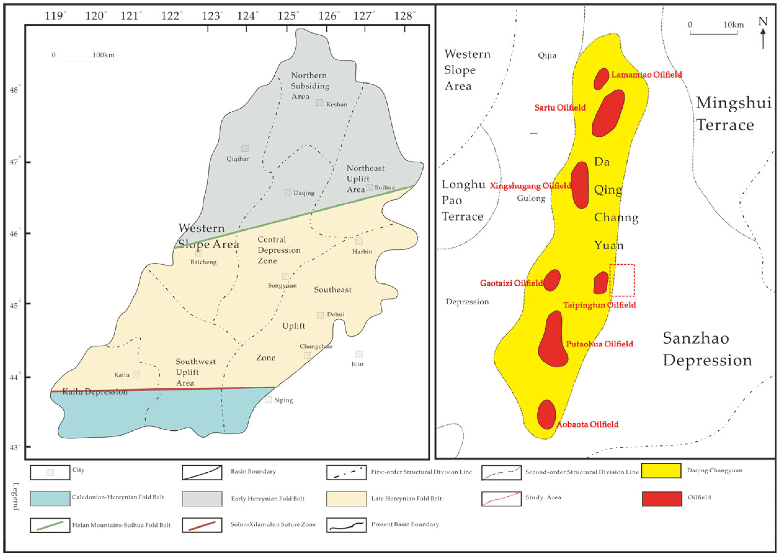
2. Geological Settings

The Weixing oilfield under study is located in Anda City, Heilongjiang Province, within the northern Songliao Basin, adjacent to Changde Town. Its tectonic setting lies in the northwestern part of the Sanzhao Depression, characterized as an uplifted structural slope belt sloping toward the Daqing Placanticline. The target reservoir, the Putaohua oil layer, belongs to the First Member of the Yaojia Formation (Cretaceous System). It was deposited during the retrogradational and fill stages of the Songliao Basin’s overall subsidence, spanning the late regressive cycle of the Qingshankou Formation to the early transgressive cycle of the Yaojia Formation. The formation is dominated by interbedded purplish-red, brownish-red, and grayish-green mudstones with grayish-white sandstones, serving as one of the major hydrocarbon-bearing formations in northern Songliao Basin [16,17]. The location of the Weixing oilfield field is shown in Figure 1.

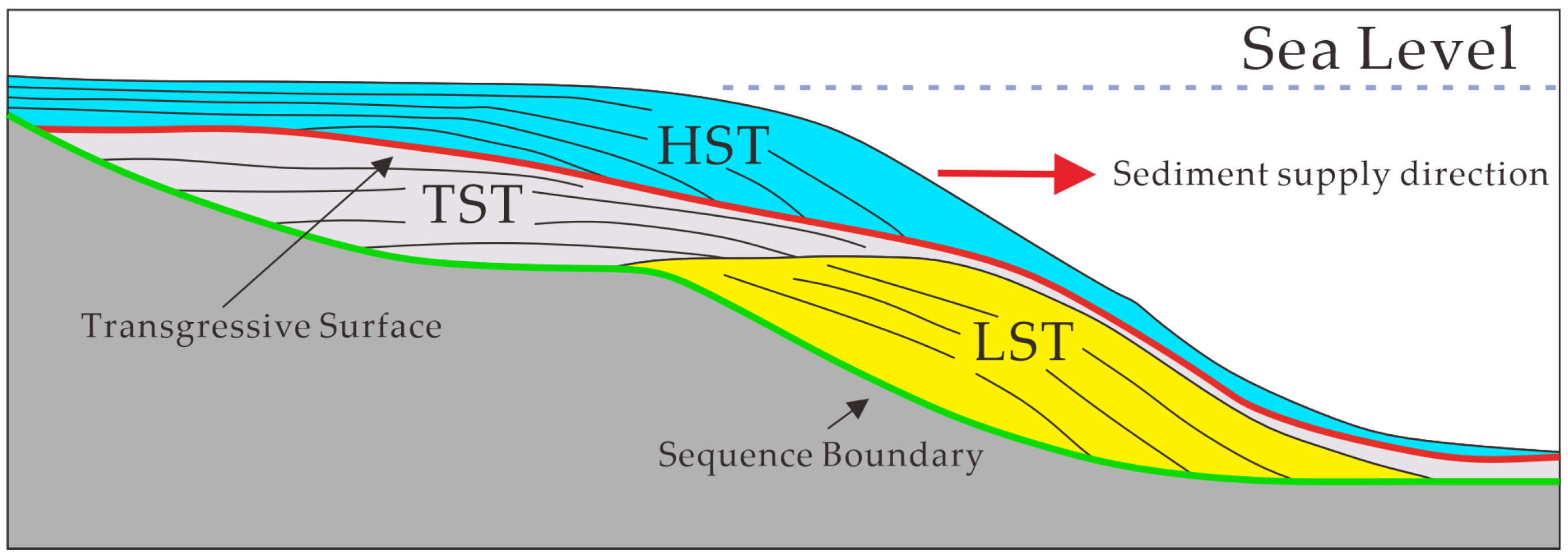
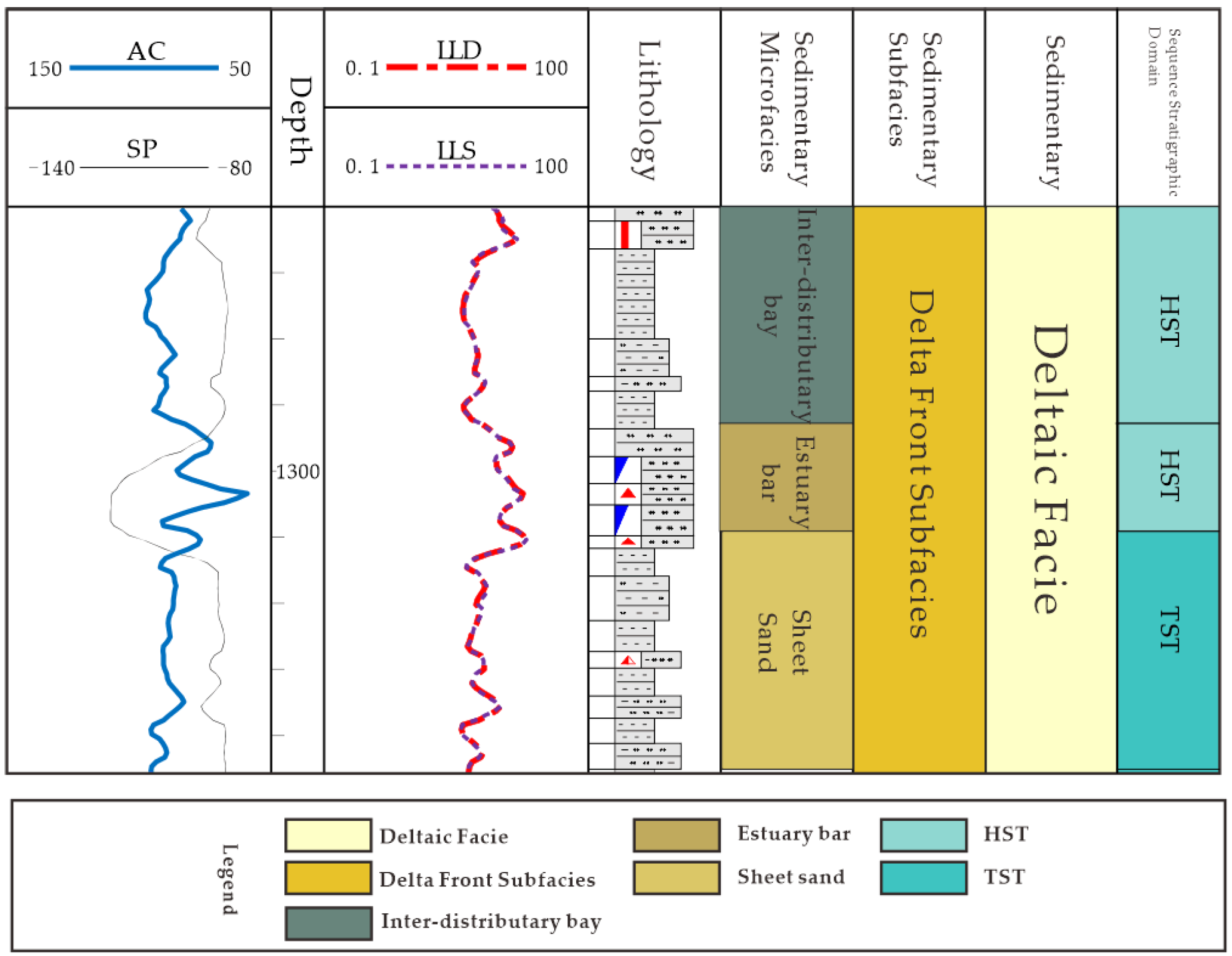
3. Characteristics of Sequences and Sedimentary Facies

The Putaohua oil layer in the study area belongs to the First Member of the Yaojia Formation (Cretaceous System), deposited during the retrogradational and fill stages of the Songliao Basin’s overall subsidence. This interval spans the late regressive cycle of the Qingshankou Formation to the early transgressive cycle of the Yaojia Formation [18,19,20]. The formation is characterized by interbedded purplish-red, brownish-red, and grayish-green mudstones with grayish-white sandstones [21].

Core-based characterization of key lithological and sedimentological features from cored wells constitutes a fundamental approach for delineating sedimentary microfacies. As the primary data source for depositional facies analysis and reservoir geological studies, detailed core observations—integrated with comprehensive well logging data analysis—enable systematic interpretation of depositional environments and facies architecture within target intervals, with a focus on diagnostic sedimentary structures. This methodology, applied across 131 wells in the Sanzhao Depression, reveals that the Putaohua oil layer represents a large-scale river-dominated shallow-water delta system. The delta is predominantly characterized by delta distributary plain and delta front subfacies, with prodelta subfacies locally developed and an absence of significant semi-deep to deep lacustrine deposits across the depression. Within this deltaic system, six sedimentary microfacies critical to reservoir–seal configurations—distributary channel, main channel, sheet sand, estuary bar, inter-distributary bay, and natural levee—are defined (representative types in

Table 1. Typical microfacies characteristics in study area and typical picture on logging groups.

Microfacies	Logging Characteristics	Thickness (m)	Typical Picture (GR SP AC LLD LLS)
Main channel	Dominated by sandstone and siltstone, the GR curve exhibits moderate–high amplitude with box-shaped or bell-shaped morphology. SP curve shows moderate–high-amplitude negative anomalies. High acoustic propagation velocity results in moderate–high AC values with morphology similar to the GR curve. Elevated resistivity yields moderate–high LLD and LLS values, also presenting box-shaped or bell-shaped patterns.	>3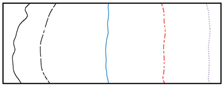
Distributary channel	Coarse-grained (predominantly gravel), the GR curve displays moderate–high amplitude with box-shaped or bell-shaped morphology. Good permeability leads to moderate–high-amplitude negative SP anomalies. Rapid acoustic wave propagation produces moderate–high AC values, mirroring the GR curve’s morphology. High resistivity generates moderate–high LLD and LLS values, consistent with GR and AC patterns.	>2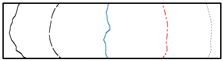
Sheet sand	Composed of well-sorted, pure sandstone, the GR curve shows moderate–high amplitude with box-shaped or bell-shaped morphology. Strong permeability causes moderate–high-amplitude negative SP anomalies. High acoustic velocity results in moderate–high AC values, matching the GR curve’s morphology. Elevated resistivity yields moderate–high LLD and LLS values, aligning with GR/AC patterns.	<1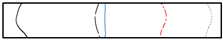
Estuary bar	Primarily fine sandstone, the GR curve exhibits low-amplitude funnel-shaped morphology. Despite sandy composition, the SP curve retains moderate–high-amplitude negative anomalies. Rapid acoustic propagation produces moderate–high AC values, though morphology transitions to funnel-shaped. High resistivity generates moderate–high LLD and LLS values, matching the funnel-shaped AC curve.	>2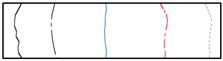
Inter-distributary bay	Clay-rich with minor siltstone and fine sand, the GR curve shows low-amplitude, high-value patterns. Poor permeability results in low-amplitude/no SP anomalies. Slow acoustic velocity leads to high-value, low-amplitude AC curves. Low resistivity yields low-amplitude LLD and LLS values.	<1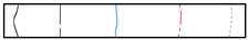
Natural levee	Thin interbeds of fine sandstone, siltstone, and mudstone display GR curves with moderate-high amplitude and box/bell-shaped morphology. Good permeability causes moderate–high-amplitude negative SP anomalies. High acoustic velocity produces moderate–high AC values, consistent with GR morphology. Elevated resistivity generates moderate–high LLD and LLS values, mirroring GR/AC patterns.	0–2

). Core data from two cored wells in the Weixing oilfield document distinct sedimentary features: lithofacies exhibit well-developed parallel and cross-bedding, alongside diagnostic subaqueous structures (e.g., lenticular and wavy bedding), with prominent scour surfaces and abrupt lithological contacts collectively indicating high-energy hydrodynamic conditions during deposition (Figure 2).

Based on the determination of sedimentary facies types, core–log calibration of key cored wells (e.g., Well W1-1-J31) must be conducted to establish a log-derived microfacies model for the entire study area, thereby providing the foundation for sedimentary microfacies mapping and subsequent analyses (Figure 3).

The classical sequence stratigraphy theory typically defines initial transgressive surfaces (ITSs) and maximum flooding surfaces (MFSs) as sequence boundaries, allowing for the identification of three major system tracts, the lowstand system tract (LST), transgressive system tract (TST), and highstand system tract (HST), as shown in Figure 4, a schematic diagram of the three major units of sequence stratigraphic domains. These tracts comprehensively document sea-level fluctuation cycles. The lowstand system tract develops at the basement of stratigraphic sequences, characterized by slow vertical aggradation and normal regression deposits [22,23]. The transgressive system tract, situated between the ITS and MFS, exhibits regressive stacking patterns due to backstepping depositional processes. In contrast, the highstand system tract overlies the TST and is dominated by progradational stratal architectures [24].

This study employs well logging curve image datasets combined with sequence system tract classifications to identify morphological characteristics of well logging facies, thereby providing critical diagnostic criteria for sedimentary microfacies recognition. For example, Figure 5 illustrates a sedimentary microfacies pattern derived from well logging facies analysis. The diagram utilizes natural gamma ray (GR), spontaneous potential (SP), acoustic (AC), laterolog deep resistivity (LLD), and laterolog shallow resistivity (LLS) curves. By integrating their morphological features with lithological data obtained from stratigraphic exploration at relative depths, a comprehensive dataset for sedimentary microfacies identification is constructed.

By integrating core, logging, and seismic data, we conducted sequence stratigraphic analysis to stratigraphically partition the 131 wells into distinct system tracts (HST, LST, and TST). Consequently, the dataset of 478 image samples was categorized accordingly: 153 samples assigned to the highstand system tract (HST), 200 to the lowstand system tract (LST), and 125 to the transgressive system tract (TST).

4. Materials and Methods

4.1. Dataset Construction

In constructing the dataset foundation for sedimentary facies recognition models, this study adopts a well logging response feature collection strategy under the framework of system tract subdivision and incorporates stratigraphic unit thickness frequency statistical methods. Based on the established sequence stratigraphic framework described earlier, well logging parameter sequences corresponding to the lowstand system tract (LST), transgressive system tract (TST), and highstand system tract (HST) were systematically collected. These parameters were stratified into four vertical thickness tiers (0–1 m, 1–2 m, 2–3 m, and >3 m) to establish feature subsets, forming a multi-scale sedimentary dynamic training dataset. First, system tract boundaries were precisely delineated through core calibration and cyclo-stratigraphic analysis. Subsequently, morphological features of five key well logging curves—natural gamma ray (GR), spontaneous potential (SP), acoustic (AC), laterolog deep resistivity (LLD), and laterolog shallow resistivity (LLS)—were extracted as well logging group images. This process yielded a standardized database containing over 2000 logging units, with LST, TST, and HST samples accounting for 42%, 26%, and 32%, respectively.

After data processing, well logging facies types were extracted by classifying distinct morphological patterns. Each morphological pattern is treated as a distinct category representing specific geological significance. By correlating these patterns with regional depositional contexts, sedimentary microfacies can be inferred. For this study, five well logging curves—natural gamma ray (GR), spontaneous potential (SP), acoustic (AC), laterolog deep resistivity (LLD), and laterolog shallow resistivity (LLS)—were selected as feature parameters due to their characteristics reflecting lithology, porosity, and sedimentary structure. These curves exhibit diverse morphologies, including composite patterns formed by combining two or more basic patterns. To facilitate machine learning analysis, numerical data from Figure 6 were converted into well logging curve images, transforming the well logging information into visual representations of logging facies.

Well logging curves exhibit distinct morphological patterns, but morphological classification inherently involves subjective interpretation, which inevitably introduces human errors. To ensure accurate morphological feature extraction and dataset construction, this study integrated domain expertise from geologists and implemented multi-expert judgment. From raw logging data of 131 wells, unambiguous morphological features were rigorously selected, followed by manual segmentation and calibration to generate 400+ training images of well logging facies types.

The integration of system tract classifications with our image dataset yielded the final dataset in

Table 2. Multiple sample points with varying thicknesses and facies.

Sample ID	Pictures					Thickness	System Tract	Microfacies
	GR 30–150 API	SP 20–120 mV	AC 500–0 µs/m	LLD 0.1–100 Ω·m(Log)	LLS 0.1–100 Ω·m(Log)
1						0.4	TST	Sheet Sand
2						0.6	TST	Main Channel
3						0.8	TST	Estuary bar
4						0.8	HST	Inter-distributary bay
5						1.2	LST	Sheet Sand
6		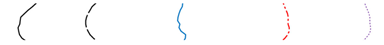				1.2	TST	Distributary channel
7						1.2	HST	Inter-distributary bay
8						1.4	LST	Main channel
9						1.6	HST	Inter-distributary bay
10						1.6	LST	Estuary bar
11						2.16	LST	Natural levee
12						2.2	LST	Distributary channel
13						3.2	LST	Sheet Sand
14						3.52	LST	Natural levee
15						4	LST	Main channel
16						4.2	LST	Estuary bar

, and the first 16 samples are shown below.

4.2. Methodology

4.2.1. Convolutional Neural Networks

Convolutional Neural Networks (CNNs) represent a paradigm shift in image classification, offering distinct advantages over traditional machine learning methods such as neural networks [3,25]. Their strength lies in discriminative feature learning, enabling noise resilience through pixel-space pattern preservation. Unlike conventional approaches that treat well logging curves as 1D data volumes for processing with Deep Neural Networks (DNNs) or 1D-CNNs, this study innovatively reinterprets log curve sets as 2D images [15,26].

Well logging curves reflect corresponding sedimentary microfacies under different depositional environments. By characterizing the variation patterns of well logging curves (amplitude characteristics, morphological features, variation trends) and integrating geological interpretations (sedimentary structures, paleocurrent directions), log facies can be systematically identified [27,28]. These log facies are further calibrated using geological data (e.g., core analysis). However, 1D data analysis, limited to numerical values, lacks the capacity to evaluate spatial correlations with neighboring samples, rendering it incapable of capturing macroscopic geological features such as textures, laminations, thin interbeds, thin overburdens, and top–bottom relationships [29,30]. Consequently, representing data as 2D images enables the capture of subtle geological information through enhanced spatial context visualization.

By leveraging 2D-CNN architectures as shown in Figure 7, we construct an intelligent sedimentary facies recognition model that integrates system tract classifications as auxiliary inputs. The model’s input dimensionality combines pixel-space features (spatial dimensions) with system tract categories, forming a novel N² + 1 dimensional dataset where N represents the logarithmic curve picture pixel resolution.

• Data preprocessing

Dataset images were acquired with uniform image resolution. Our dataset was partitioned into training (70%) and testing (30%) subsets. To preserve geological details, preprocessing and dynamic augmentation were implemented to enhance data diversity while maintaining stratigraphic fidelity for model training.

Due to stratigraphic thickness variations causing significant disparities in pixel dimensions across images, excessive thickness leads to severe stretching of thin-layer images (resulting in distortion), while insufficient thickness compresses thick layers, causing substantial loss of geological information. To address this, we implemented a thickness-based classification strategy. Based on statistical analysis of our training samples, the dataset was categorized into four stratigraphic thickness classes: >3 m, 2–3 m, 1–2 m, and <1 m.

To resolve multi-scale representation challenges in geological bodies, this study proposed a thickness-adaptive input sizing algorithm based on seismic reflection thickness. Thickness metadata parsed from filenames automatically classified strata into four granularity levels (0–1 m, 1–2 m, 2–3 m, >3 m), corresponding to input resolutions of 64 × 64, 128 × 128, 192 × 192, and 256 × 256, respectively. This design captured fine-scale laminae with small resolutions and preserved macro-scale structures with large resolutions, achieving resampling via bilinear interpolation combined with centered cropping via zero-padding.

To address the spatial heterogeneity of sedimentary facies images, this study designed a three-stage augmentation framework incorporating geometric transformations, illumination perturbations, and domain adaptation (Figure 8). The geometric transformation module employs random rotations (±45°), non-uniform translations (horizontal/vertical offsets: 0.3× image dimensions), scale adjustments (0.6–1.5×), and shear deformations (0.3 radians), simulating geometric distortions during seismic wave propagation via affine transformation matrices. The illumination perturbation module introduces brightness range modulation (0.5–1.5×) and contrast enhancement (0.7–1.3×) to emulate imaging variations under different lighting conditions. Notably, a class-specific augmentation intensity adjustment mechanism was developed for underrepresented categories (e.g., main channels, natural levees): dynamically tuning brightness perturbation magnitudes (1.2× enhancement for channels, 1.5× for levees) to increase sample diversity while preserving geological semantics.

• Hyperparameter optimization

Hyperparameters are parameters that influence the training-derived parameters and are associated with the model algorithm. The selection of hyperparameters requires manual input and adjustment by the practitioner to optimize model performance. We employed a pipeline mechanism to systematically configure preprocessing and 2D-CNN hyperparameters within predefined optimal ranges. By analyzing classifier outputs, we identified the optimal hyperparameter combinations corresponding to the best performance, thereby achieving optimal hyperparameter configuration for the model. The hyperparameter optimization results are summarized in

Table 3. The hyperparameter optimization results.

Hyperparameter Category	Parameter Name	Value/Configuration
Data Preprocessing	Rotation Range	±45°
	Width Shift Range	0.3
	Height Shift Range	0.3
	Zoom Range	[0.6, 1.5]
	Shear Range	0.3
	Brightness Range	[0.5, 1.5]
	Horizontal Flip	True
	Class-specific Enhancement	Main Channel: ×1.2 Natural Levee: ×1.5
Model Architecture	Input Size (Dynamic)	0: (64 × 64) 1: (128 × 128) 2: (192 × 192) 3: (256 × 256)
	Convolutional Layer 1	Filters = 16, Kernel Size = (3 × 3), Activation = ‘relu’, Padding = ‘same’
	Convolutional Layer 2	Filters = 32, Kernel Size = (3 × 3), Activation = ‘relu’, Padding = ‘same’
	Dense Layer (Feature Fusion)	Units = 8, Activation = ‘relu’
	Output Layer	Units = 6, Activation = ‘softmax’
	Dropout	Rate = 0.5

.

Our model employed five key optimization strategies: (1) thickness-adaptive input scaling (64 × 64 to 256 × 256) to preserve geological features across bed thicknesses; (2) class-specific augmentation intensities to address imbalance; (3) dual-rate learning scheduling (initial 1 × 10⁻³ with exponential decay and plateau detection); (4) a balanced dual-input architecture (3 convolutional blocks + 2 dense layers) with concatenation-based fusion; (5) automated class weighting. These choices were informed by iterative ablation and validated through 5-fold cross-validation. The configuration balances computational efficiency with geological plausibility, particularly for underrepresented facies like channels.

4.2.2. The Workflow of the Proposed Approach

This study systematically addresses the challenges of multi-scale feature extraction and small-sample class recognition in sedimentary facies image classification through the development of a lightweight convolutional neural network (CNN) integrating multi-scale dynamic inputs and cross-modal fusion with sequence stratigraphic analysis. The experimental workflow comprises four core components: data preprocessing, augmentation strategy design, model architecture optimization, and performance evaluation.

The model architecture adopts a lightweight dual-branch design:

(1) The image input branch contains three convolutional modules (32 → 64 → 128 channels), extracting local texture features via dynamic convolution kernels, combined with global average pooling to compress spatial dimensions;

(2) The system tract input branch embeds prior geological knowledge (system tract classifications) through fully connected layers. These features are concatenated with image features along the channel dimension before final classification via fully connected layers into six sedimentary facies probabilities. To suppress overfitting, a dropout layer (rate 0.5) is introduced before fully connected layers, supplemented by L2 regularization constraints post convolution. The optimizer employs the Adam algorithm with an initial learning rate set to 1 × 10⁻³, dynamically adjusted via an exponential decay strategy (decay rate 0.9, step size 500). The loss function utilizes weighted cross-entropy, addressing class imbalance through computed class weights.

Experimental evaluation employs five-fold cross-validation, with primary metrics including overall accuracy, the Jaccard similarity coefficient, and the Matthews correlation coefficient. Feature space distributions are analyzed via confusion matrices and t-SNE-based dimensionality reduction visualization to verify the model’s discrimination capability between thin-bed channels (<1 m) and thick-bed shoals (>3 m).

The overall procedure of the proposed method is shown below in Figure 9.

4.2.3. Implementation Details

The codebase was developed in Python 3.10, utilizing TensorFlow 2.15 and Keras 3.0 for neural network implementation. Data preprocessing and augmentation pipelines relied on OpenCV 4.8.0, Numpy 1.24.0, and TensorFlow’s ImageDataGenerator 2.15 for dynamic resizing, normalization, and data augmentation (e.g., rotation, zoom, brightness adjustment). Geological image-specific preprocessing included adaptive input scaling based on seismic reflection thickness (64 × 64 to 256 × 256 pixels) and cross-modal feature fusion with domain knowledge embedding. Computations were accelerated on an NVIDIA GeForce RTX 3060Laptop GPU (6 GB) 576.80, enabling efficient training of lightweight architectures with mixed-precision optimization.

5. Results and Discussion

5.1. Models Evaluation

For facies classification, evaluation metrics encompass accuracy and similarity-based measures, such as the Jaccard similarity score (ranging from 0 to 1, where values closer to 1 indicate higher prediction accuracy) and the Matthews correlation coefficient (MCC) (ranging from −1 to 1, where 1 represents perfect prediction, 0 indicates random guessing, and −1 denotes total inversion). These measures are essential for evaluating the performance of the CNN model in classifying facies accurately and effectively.

In addition to these measures, the confusion matrix serves as a comprehensive evaluation tool, providing a detailed breakdown of the model’s performance across different classes. This tool is particularly useful for identifying any potential biases in the model’s predictions, which can be addressed through further optimization and fine-tuning.

The model evaluation results for the CNN-2D architecture are presented in

Table 4. Model evaluation metrics results.

Metrics	Jaccard Similarity Coefficient	Matthews Correlation Coefficient	Number of Samples	Average Accuracy
Training Set	0.890081	0.9220971	334	0.8913
Test Set	0.894478	0.906416	144	0.8349

, which provides a comprehensive overview of the performance metrics for this model.

The results of the model evaluation using cross-validation are shown in

Table 5. Cross-validation model evaluation results.

Metrics	Cross-Validation Fold 1	Cross-Validation Fold 2	Cross-Validation Fold 3	Cross-Validation Fold 4	Cross-Validation Fold 5	Mean
Training Set	0.8879	0.7916	0.8045	0.8084	0.8294	0.8243

.

The model exhibits high accuracy on both training and test datasets, achieving average accuracies of approximately 89.13% and 83.49%, respectively, indicating strong overall performance. Jaccard similarity coefficients remain elevated (>0.89) across both datasets, demonstrating substantial overlap between predicted boundaries and ground-truth labels. While the test set achieves marginally higher average accuracy (0.894478 vs. 0.906416), the difference is negligible. Conversely, the training set displays significantly higher Matthews correlation (0.9220971 vs. 0.906416 for the test set), suggesting slight overfitting to the training data. In conclusion, the model demonstrates robust performance but retains room for optimization to enhance generalization capabilities.

We implemented standard 5-fold cross-validation with randomized sample allocation to ensure robust performance evaluation while maintaining computational efficiency. The choice of 5 folds was deliberate to provide sufficient training data in each split given our limited sample size and yield more stable performance estimates, as 2-fold validation would halve the training set and potentially introduce higher variance in results. This approach aligns with common practice in machine learning studies with medium-sized datasets.

The average accuracy on the training set is 0.8243 (approximately 82.43%), indicating that the model performs well overall. Fold 1 performs significantly better than the other folds, while Fold 2 performs relatively weaker. Overall, the model performs well, but the performance differences among the folds need attention to ensure the reliability and generalization ability of the model.

The issue of imbalanced class distribution in datasets can be addressed through oversampling techniques. Oversampling involves replicating instances from the minority class while maintaining the original quantity of majority class samples, thereby achieving a more balanced distribution between classes. Additionally, model training can be further optimized by assigning appropriate weights to samples from different classes. It is important to note that conventional random oversampling, which simply duplicates minority class samples, may lead to model overfitting. Therefore, in practical applications, we will prioritize model architectures with robust anti-overfitting capabilities and incorporate more advanced oversampling methods (such as SMOTE) to enhance model performance.

The confusion matrix experimental results shown in Figure 10 indicate that the classification model exhibits excellent performance in certain categories while facing significant challenges in others. Overall, the model demonstrates high prediction accuracy for “Distribution channel”, “Inter-distributary bay”, and “Sheet sand”, reflecting strong feature extraction capabilities. Due to the similarities in well logging curves between main channels and distributary channels, a portion of distributary channel images were misclassified as main channels. In the deltaic facies, the main channel and distributary channel are located within the delta plain, and their depositional environments are similar. Both have similar lithofacies characteristics, mainly composed of sandstone, with upward-fining sedimentary sequences, and they commonly develop tabular and trough cross-bedding with asymmetric ripple marks and scour-fill structures. However, there are differences in thickness variations and well logging curve morphologies between the main channel and distributary channel. The main channel is usually thicker than the distributary channel, and its well logging curves typically show high-amplitude bell or box shapes, while the distributary channel’s well logging curves may show low-amplitude bell or box shapes. The inter-distributary bay, characterized by uniquely identifiable well logging curves, achieved the highest recognition accuracy. In this study, the limited sample size of natural levee samples led to occasional recognition difficulties. However, the overall model performance underscores its reliability in identifying dominant depositional facies.

As depicted in Figure 11, the loss curves demonstrate that both training and validation losses decreased rapidly within the first five training epochs. By epoch 35, the training loss dropped to approximately 0.04, while the validation loss remained at around 0.42. The relatively close proximity of the two curves indicates strong generalization capabilities with no severe overfitting. The accuracy curves reveal an initial low accuracy that improved significantly during training. The training accuracy ultimately reached 0.85, while the validation accuracy stabilized at 0.75. Overall, the CNN model exhibits effective training performance characterized by continuous loss reduction, steady accuracy improvement, and minimal divergence between training and validation metrics, confirming robust generalization ability.

The learning curve graph illustrated in Figure 12 shows the variation trends of the training accuracy (depicted by the blue line) and validation accuracy (depicted by the red line) during the model’s training process. The training accuracy rapidly increased from an initial low value to around 0.8, and while experiencing slight fluctuations, it continued to rise steadily, reaching nearly perfect accuracy of 1.0 by the 55th training epoch. Meanwhile, although the validation accuracy improved in tandem, it consistently fluctuated around 0.6–0.7 without surpassing this upper limit. The divergence between these two curves indicates mild overfitting in the model, though the overall performance remains satisfactory.

In Figure 13, the different depositional environments (such as the purple cluster of distributary channels and the red cluster of natural levees) form relatively independent clusters in the 2D space, indicating that the model has captured key differences in geological features. This separation holds important reference value for sedimentary facies identification research. The dispersed distribution of data points near the sheet sand may reflect transitional characteristics between the sheet sand and adjacent environments, and such detailed representations are helpful for understanding the boundaries of depositional systems.

5.2. Models Performance

By integrating single-well facies diagrams and analyzing a subset of representative samples, we conducted analytical validation of the final CNN-2D model’s outcomes.

Figure 14 illustrates the sedimentary sequence in the depth interval of 1170–1218 m for Well W2-18-10, characterized by a transition from the lowstand system tract to the transgressive system tract, with sedimentary bodies evolving from channel deposits to thin sandstones. Within the depth range of 1190–1194 m, the measured depositional facies is sheet sand, but the model misclassifies it as a natural levee. Additionally, at depths of 1214–1216 m, the actual depositional facies is a main channel, yet the model erroneously assigns it to a distributary channel. These misclassifications primarily stem from discrepancies between resistivity response characteristics and microfacies attributes, potentially caused by GR curve noise interference due to wellbore enlargement or insufficient model sensitivity to the difference between deep and shallow resistivity measurements (LLD/LLS).

Figure 15 illustrates the stratigraphic interval from 1200 to 1250 m of Well W2-21-19, which represents a depositional sequence from the lowstand system tract. The overall sedimentary body is dominated by thick channel deposits. Notably, the basal sheet sand is predicted with high accuracy, while the intermediate strata show prediction bias where distributary channels were misidentified as main channels, and sheet sands were erroneously interpreted as natural levees. The upper channel recognition remains relatively accurate. The sample misclassifications primarily stem from SP curve distortions caused by multiple interfering factors, compounded by wellbore enlargement-induced noise that disrupts curve imaging. Overall, the interpretation demonstrates satisfactory reliability despite localized inaccuracies.

6. Conclusions

This study presents a novel approach for intelligent sedimentary facies identification by integrating multi-resolution sequence stratigraphy with deep learning techniques. The proposed framework effectively addresses the challenges of multi-scale geological feature extraction and small-sample-class imbalance through dynamic input adaptation and cross-modal feature fusion. Experimental results demonstrate that the hybrid model achieves an overall classification accuracy of 83%, with accuracy exceeding 80% for thin-bedded lithofacies (<1 m) and thick-bedded systems (>3 m) (Figure 16).

The method significantly improves interpretative efficiency while maintaining geological plausibility, offering a scalable solution for high-resolution subsurface characterization in complex depositional environments. Future work will focus on incorporating 3D spatial continuity constraints and real-time processing capabilities for field-scale applications.

7. Future Work

Despite the promising results achieved by the current model, potential overfitting issues may arise due to the limited sample size, high-dimensional feature space, or suboptimal model complexity. To mitigate this risk and further enhance generalization performance, the following directions are proposed for future work:

• Expanding the dataset: collecting more representative samples will help improve model robustness and reduce overfitting caused by data scarcity.
• Feature selection and dimensionality reduction: techniques such as PCA, L1 regularization (Lasso), or mutual information-based selection will be explored to eliminate redundant or irrelevant features, thereby simplifying the model.
• Data structure optimization: reconstructing input data by incorporating domain knowledge or hierarchical representations may enhance feature discriminability.
• Model complexity adjustment: adopting more sophisticated architectures could better balance bias–variance trade-offs.

These improvements aim to build a more reliable and generalizable framework for real-world applications.

References

- Deng, F.; Meng, R. On Logging Curves Fine Delamination to Identify Sedimentary Microfacies. Well Logging Technol. 2010, 34, 554–558. [Google Scholar]
- Edmonds, D.A.; Slingerland, R.L. Significant Effect of Sediment Cohesion on Delta morphology. Nat. Geosci. 2009, 3, 105–109. [Google Scholar] [CrossRef]
- Zhao, C.; Jiang, Y.; Wang, L. Data-Driven Diagenetic Facies Classification and Well-Logging Identification Based on Machine Learning Methods: A Case Study on Xujiahe Tight Sandstone in Sichuan Basin. J. Pet. Sci. Eng. 2022, 217, 110798. [Google Scholar] [CrossRef]
- Wei, L. The Theory and Study on Logging Facies Analysis. Master’s Thesis, Chengdu University of Technology, Chengdu, China, 2002. [Google Scholar]
- Yong, S.; Wen, Z. Quantitative Discrimination of Sedimentary Microfacies with Bayes Discrminant Analysis. Well Logging Technol. 1995, 19, 22–27. [Google Scholar]
- Bhatt, A.; Helle, H.B. Determination of Facies from Well Logs Using Modular Neural Networks. Pet. Geosci. 2002, 8, 217–228. [Google Scholar] [CrossRef]
- Saggaf, M.M.; Nebrija, E.L. A Fuzzy Logic Approach for the Estimation of Facies from Wire-Line Logs. AAPG Bull. 2003, 87, 1223–1240. [Google Scholar] [CrossRef]
- Lu, S.; Pan, H.; Shuguang, P. Auto-Identified System and Study of Sedimentary Microfacies and Elextrofacies Taking Snaking Stream Deposition as an Example. Chin. J. Eng. Geophys. 2009, 6, 332–337. [Google Scholar]
- Wu, C.; Li, Z. Logging Facies Analysis and Sedimentary Facies Identification Based on Bp Neural Network. Coal Geol. Explor. 2012, 40, 68–71. [Google Scholar]
- Xu, H. Research on Logging Facies Recognition Method Based on Convolutional Neural Network. Master’s Thesis, China University of Petroleum, Beijing, China, 2019. [Google Scholar]
- Wang, D.; Peng, J.; Yu, Q.; Chen, Y.; Yu, H. Support Vector Machine Algorithm for Automatically Identifying Depositional Microfacies Using Well Logs. Sustainability 2019, 11, 1919. [Google Scholar] [CrossRef]
- Gao, H. The Recognition of the Sedimentary Facies Based on Well Logging Curves. Master’s Thesis, Wuhan Institute of Technology, Wuhan, China, 2014. [Google Scholar]
- Yadigar, I.; Sukhostat, L. Lithological Facies Classification Using Deep Convolutional Neural Network. J. Pet. Sci. Eng. 2019, 174, 216–228. [Google Scholar]
- Li, W.B.; Yu, Y.L.; Wang, J.Q.; Bai, Y.; Wang, X. Application of Self-Organizing Neural Network Method in Logging Sedimentary Microfacies Identification. Adv. Mater. Res. 2012, 616–618, 38–42. [Google Scholar] [CrossRef]
- Zhang, J.; Liu, S.; Li, J.; Liu, L.; Liu, H.; Sun, Z. Identification of Sedimentary Facies with Well Logs: An Indirect Approach with Multinomial Logistic Regression and Artificial Neural Network. Arab. J. Geosci. 2017, 10, 247. [Google Scholar] [CrossRef]
- Ye, Y. The Result and Knowledge of the Putaohua Reservoir Old Well Reexamination in Weixing Oilfield. Value Eng. 2013, 32, 291–292. [Google Scholar]
- Wang, W.; Cui, Y.; Wu, Y.; Deng, Q.; Zhou, L.; Liu, Q.; Qin, Y.; Qiu, Z. Seismic Prediction of Thin Channel Sand Body Based on Data Mining and Optimization: A Case Study of Fui I Oil Group in Weixing Oilfield, Northern Songliao Basin. J. Chengdu Univ. Technol. (Sci. Technol. Ed.) 2023, 50, 385–400. [Google Scholar]
- Liu, Z.; Dong, Z.; Liu, X.; Pan, G.; Zhao, G.; Huang, J. Precise Description of Underwater Distributary Channel of Putaohua Reservoir in Weixing Oil Field, Sanzhao Sag. J. Heilongjiang Univ. Sci. Technol. 2021, 31, 272–278. [Google Scholar]
- Qin, Y. Main Controlling Factors and Reservoir Formation Mode of Oil and Gas in the Putaohua Reservoir in Sanzhao Sag, Songlliao Basin. Spec. Oil Gas Reserv. 2023, 30, 28–34. [Google Scholar]
- Liu, Z.; Li, X.; Zheng, R.; Liu, H.; Yang, Z.; Cao, S. Sedimentary Characteristics and Models of Shallow Water Delta Front Subfacies Reservoirs: A Case Study of Sapugao Oil Layer in North- Ii Block of Sabei Oilfield, Daqing Placanticline. Lithol. Reserv. 2022, 34, 1–13. [Google Scholar]
- Sun, Y.; Yu, L.; Yan, B.; Liu, Y.; Cong, L.; Ma, S. Oil-Water Distribution and Its Major Controlling Factors of Putaohua Reservoir of the Cretaceous Yaojia Formation in Syncline Area of Sanzhao Sag, Songliao Basin. Oil Gas Geol. 2018, 39, 1120–1130+1236. [Google Scholar]
- Zhu, X.; Wang, H.; Zhu, H.; Shao, L.; Ji, Y. Research Progress and Development Focuses of Continental Sequence Stratigraphy. Acta Pet. Sin. 2023, 44, 1382–1398. [Google Scholar]
- Posamentier, H.W.; Allen, G.P.; James, D.P.; Tesson, M. Forced Regressions in a Sequence Stratigraphic Framework: Concepts, Examples, and Exploration Significance. AAPG Bull. 1992, 76, 1687–1709. [Google Scholar]
- Helland-Hansen, W.; Gjelberg, J.G. Conceptual Basis and Variability in Sequence Stratigraphy: A Different Perspective. Sediment. Geol. 1994, 92, 31–52. [Google Scholar] [CrossRef]
- Zhu, L.; Li, H.; Yang, Z.; Li, C.; Ao, T. Intelligent Logging Lithological Interpretation with Convolution Neural Networks. Petrophys.—SPWLA J. Form. Eval. Reserv. Descr. 2018, 59, 799–810. [Google Scholar] [CrossRef]
- Blanco, V.M.; Bom, C.R.; Coelho, J.M.; Correia, M.D.; de Albuquerque, M.P.; de Albuquerque, M.P.; Faria, E.L. A Deep Residual Convolutional Neural Network for Automatic Lithological Facies Identification in Brazilian Pre-Salt Oilfield Wellbore Image Logs. J. Pet. Sci. Eng. 2019, 179, 474–503. [Google Scholar]
- Alzubaidi, F.; Mostaghimi, P.; Swietojanski, P.; Clark, S.R.; Armstrong, R.T. Automated Lithology Classification from Drill Core Images Using Convolutional Neural Networks. J. Pet. Sci. Eng. 2021, 197, 107933. [Google Scholar] [CrossRef]
- Han, H.; Wang, J.; Kang, Y.; Feng, D.; Liu, H.; Zhu, J.L.; Yu, W. Research Status and Prospect of Intelligent Logging Processing and Interpretation Methods. J. China Three Gorges Univ. (Nat. Sci.) 2022, 44, 1–14. [Google Scholar]
- Hall, B. Facies Classification Using Machine Learning. Lead. Edge 2016, 35, 906–909. [Google Scholar] [CrossRef]
- Yin, C.; Liu, W.; Yang, H.; Cao, M. Advances in Foreign Well Logging Technology Development. World Pet. Ind. 2024, 31, 77–87. [Google Scholar]