Error Model for Autonomous Global Positioning Method Using Polarized Sky Light and True North Measurement Instrument

Abstract

Long-distance navigation requires global positioning methods to have complete autonomy, particularly when the Global Positioning System is unavailable. Considering that bionic polarized light-based global positioning technology exhibits good autonomy, this study develops an error model for autonomous global positioning based on the polarized skylight and a true north measurement instrument, using an approach of partial derivatives. The proposed model can rapidly and accurately provide the global error distribution of a bionic positioning method under varying angular measurement errors at different times. In addition, the conditions under which the proposed error model remains valid are investigated. The results indicate that the investigation can be simplified to verify whether the denominators of four partial derivatives of an implicit function system are simultaneously non-zero. The accuracy of the proposed error model is verified through numerical simulations. The results indicate that when the deviations of the two independent variables are up to 0.0001°, the positioning error mostly remains less than 14 m. In contrast, fewer geographical locations have positioning errors approaching positive infinity. By analyzing the global error distribution, one can effectively design and optimize the parameters of the autonomous global positioning system, enhancing its reliability and stability.

1. Introduction

In long-distance navigation tasks, the use of global positioning technology is necessary. Current global positioning technologies mainly include satellite navigation technology and inertial navigation technology. Satellite navigation technology has been extensively implemented into various transportation vehicles, including aircraft, maritime vessels, and automobiles. However, satellite signals are man-made and are susceptible to interference, particularly under extreme conditions, such as in Global Positioning System (GPS)-denied environments. In addition, the positioning error in inertial navigation accumulates over time.

Bionic polarized light-based global positioning technology can effectively overcome the two limitations of satellite navigation and inertial navigation technologies. It employs a completely autonomous global positioning approach without error accumulation. The exploration of this technology can be traced back to 1947, when Frisch et al. reported that bees could perceive polarized light in the atmosphere [1], prompting scientific inquiry into bionic polarized light navigation. Lambrinos et al. focused on the compound eye structure of insects [2]. Over several decades, researchers have developed a comprehensive understanding of the way various organisms use polarized light from the sky to obtain information on orientation. In 1997, Rüdiger and Dimitrios developed a sky polarized light compass and performed trajectory control experiments using a four-wheeled robot [3,4]. Chu et al. (2005) investigated the polarized light sensitivity model of insect compound eyes [5] and analyzed its angle measurement mechanism model in detail, subsequently developing a heading measurement sensor [6]. Chahl and Mizutani (2012) developed and calibrated a polarized light compass and conducted flight tests on a fixed-wing drone; the results demonstrated that the heading accuracy was comparable to that of a traditional magnetic compass [7]. Further, in 2012, Ropars et al. reported that ancient Vikings might have employed calcite to detect polarized light in the sky for navigational purposes [8]. Horváth et al. analyzed the errors in the three navigation steps in detail for using polarized light like the Vikings [9,10,11]. The simulation results derived from extensive observational data suggested that it was indeed plausible for the Vikings to navigate from Norway in Northern Europe to Greenland using polarized light information from the sky [12]. In summary, previous studies have enabled researchers to derive heading information by detecting polarization data from scattered atmospheric light [13].

However, there are significant distinctions between the long- and short-distance movements along the Earth’s surface. For short distances, such as 3 km, the destination can be seen. In contrast, for long distances, like 1000 km, the destination is out of sight from the starting point. When navigating over bodies of water or through the atmosphere, one might experience yaw because of the influence of water currents and airflows. Due to this phenomenon, it is necessary to perform continuous course adjustments according to one’s global position. Therefore, it is insufficient to attain orientation only, and advancing global positioning technology is imperative.

The technology of polarized light navigation has progressively transitioned in recent years from obtaining the heading to obtaining the global position. Wang and Chu (2015) developed an autonomous real-time global positioning navigation method based on the Earth’s sky polarized light and magnetic field [14]. Mei et al. (2015) designed a non-real-time autonomous global positioning method [15], which relies exclusively on the Earth’s sky polarized light and requires at least two independent observations of the sky. However, both studies simulated positioning errors for specific times and locations without addressing the variability of errors across different times and geographical locations globally. Gruev et al. (2018) introduced a non-real-time autonomous global positioning method using underwater polarized light [16]. Their research involved the development of an innovative biomimetic underwater polarized light detection camera, which was validated for its positioning capabilities across various geographical locations on the Earth. Guo et al. further advanced this field by employing the time differential polarization field to minimize errors in underwater polarization detection [17]. Yang et al. (2021) developed a non-real-time global positioning method [18], which determines global positions based on the distribution of the polarization degree of sky polarized light; in contrast, the previous studies were based on the polarization angles of sky polarized light. Viollet et al. (2023) suggested a method that uses the temporal characteristics of the Earth’s sky polarized light and employs a polarization camera to measure this light [19,20]. This method calculates the geographic north direction and an observer’s latitude. When combined with additional navigation data, this method can facilitate the global positioning process. Hu et al. (2024) developed an integrated navigation system combining multi-directional polarization sensors [21], a sun sensor, and an inertial measurement unit (IMU). Moutenet et al. (2024) designed a publicly available detection device computer program [22], thus promoting international collaboration in advancing polarized navigation technology.

Based on their fundamental principles, global positioning methods can be roughly classified into two distinct categories. The first category uses sky scattering light detection devices and geographic true north information detection devices simultaneously. First, the solar azimuth and elevation angles, defined in the body coordinate system, are derived from the polarization information [23,24], including the angle or degree of polarization of the scattered light. This information is then combined with the heading information provided by a geographic true north information detection device to determine the solar elevation and azimuth angles at the carrier’s location. Finally, the geographic location of the carrier is obtained. This approach has real-time capability and necessitates only a single detection of sky-scattered light.

The second category relies only on the sky-scattered light detection device, and the solar azimuth and elevation angles, defined in the body coordinate system, are determined based on the polarization information of the scattered light. However, due to the inability to obtain the true north heading of the carrier from a single observation, this category requires at least two observations to be performed to determine the carrier’s geographic location. Consequently, these methods are classified as non-real-time methods, and if the time interval between the two measurements is very short, the precision of the geographic localization can decrease.

Existing research suggests that the global positioning methods based on polarized light both provide global positioning functionality and maintain the autonomy of methods, meaning that they do not rely on any artificial signals. However, research on the positioning errors of these methods has been relatively scarce [25], particularly regarding the global distribution patterns of positioning errors at different times and under different error conditions.

Aiming to address the current shortcomings, this paper designs a global error model for the real-time global positioning methods. The proposed model can rapidly and accurately provide the global distribution patterns of positioning errors at different times and under different error conditions. It can also serve as a theoretical framework for navigation task planning, thus enabling the avoidance of non-linear regions where minor measurement inaccuracies might result in substantial positioning discrepancies. Furthermore, the design and development of polarized light sensors and cameras can be determined by the proposed error model. For instance, the positioning accuracy of the GPS is typically within the meter range. Further, the autonomous positioning error model can determine the precision required for measurements of polarized angles, thus enabling the autonomous positioning method to achieve meter-level accuracy. In summary, by analyzing the global error distribution, one can effectively design and optimize the parameters of the autonomous global positioning system, enhancing its reliability and stability.

This paper is organized as follows: Section 2 introduces the fundamental principles of real-time global positioning methods. Section 3 develops the error model by employing partial derivatives and outlines the conditions under which the proposed error model is valid. Section 4 verifies the accuracy of the proposed error model through numerical simulation. Finally, Section 5 summarizes the spatial and temporal distribution properties of the proposed error model.

2. Autonomous Global Positioning Method

An autonomous global positioning system based on the Earth’s sky polarized light and a true north measurement instrument generally includes several polarized light sensors, a true north measurement device, and a computer. The global position calculation flowchart of an autonomous global positioning system is presented in Figure 1.

The specific steps of the global position calculation flowchart are as follows. First, a polarization light sensor measures the scattered light in the atmosphere to obtain a polarization vector e. The orthogonal vector algorithm [24] obtains a solar vector S_b in the body coordinate system. Then, the three altitude angles provided by a true north measurement instrument are used to determine a solar vector S_n in the East–North–Up (ENU) coordinate system. Next, the solar altitude angle and the solar azimuth angle are calculated. Further, the Coordinated Universal Time (UTC) is obtained from the clock integrated into a computer; this allows for the retrieval of the corresponding solar declination and solar time difference based on the UTC and the astronomical calendar. Finally, this information is substituted into the system of equations of a global positioning method to obtain the global position of the carrier.

2.1. Global Positioning Method Equation System

The system of equations of the global positioning method is defined as follows:

$$\cos A_{\mathrm{s}}={\displaystyle \frac{\sin \delta -\sin h_{\mathrm{s}}\sin \psi }{\cos h_{\mathrm{s}}\cos \psi }},$$

(1)

$$\sin h_{\mathrm{s}}=\sin \psi \sin \delta +\cos \psi \cos \delta \cos (\eta +(UTC+E_{\mathsf{\omega }})\times 15°-180°),$$

(2)

where A_s is the solar azimuth angle; h_s is the solar altitude angle; δ is the solar declination; ψ is the geographic latitude; η is the geographic longitude; E_ω is the difference between the true and mean solar hours; UTC is the UTC value; and ω is the solar hour angle, which is calculated by $\eta +(UTC+E_{\mathsf{\omega }})\times 15°-180°$.

The heading angle (Y), pitch angle (P), and roll angle (R) are determined using a true north measurement device. A three-dimensional rotation matrix created by the three angles is defined by Equation (3). This matrix can be used to convert a vector from the body coordinate system to the ENU coordinate system. The body coordinate system O_bX_bY_bZ_b is defined as follows. The coordinate origin is set at the center of gravity of a vehicle; the x-axis points to the right side of the vehicle; the y-axis points to the front of the vehicle; and the z-axis is perpendicular to the vehicle pointing upwards, forming a right-handed coordinate system. The ENU coordinate system O_nX_nY_nZ_n is defined as follows. The origin of this coordinate system is set at the observation point, the x-axis points to true east, the y-axis points to true north, and the z-axis is perpendicular to the horizontal plane, pointing upwards, also forming a right-handed coordinate system.

$${\mathit{C}}_n=\left[\begin{array}{ccc}\cos Y& \sin Y& 0\\ -\sin Y& \cos Y& 0\\ 0& 0& 1\end{array}\right]\left[\begin{array}{ccc}1& 0& 0\\ 0& \cos P& -\sin P\\ 0& \sin P& \cos P\end{array}\right]\left[\begin{array}{ccc}\cos R& 0& \sin R\\ 0& 1& 0\\ -\sin R& 0& \cos R\end{array}\right].$$

(3)

A solar vector obtained from the polarization information of polarized sky light is denoted by S_b and defined in the body coordinate system. The solar vector in the ENU coordinate system is expressed as follows:

$${\mathit{S}}_n={\mathit{C}}_n{\mathit{S}}_b=\left(\begin{array}{c}{S}_x\\ S_y\\ S_z\end{array}\right)=\left(\begin{array}{c}\cos h_{\mathrm{s}}\sin A_n\\ \cos h_{\mathrm{s}}\cos A_n\\ \sin h_{\mathrm{s}}\end{array}\right).$$

(4)

Using Equation (4) and the solar altitude angle value, a solar altitude angle h_s and an azimuth angle A_n in the ENU coordinate system can be determined. The solar azimuth angle is defined in the plane formed by X_n and Y_n, with the geographic true north direction (Y_n) as a reference direction and clockwise as positive; therefore, it holds that

$$A_{\mathrm{s}}=90°-A_n.$$

(5)

The autonomous global positioning method determines the global position of the carrier by solving the system of equations formed by Equations (1) and (2). This study aims to develop a global error model that can provide the global distribution of deviations in the geographic longitude and latitude, which are caused by the measurement angle errors of the two independent variables at different times. In addition, this study aims to translate the angle errors of the geographic longitude and latitude (expressed in degrees) into the corresponding distance errors of the Earth’s surface (expressed in kilometers).

2.2. Number of Solutions to Global Positioning Method Equation System

Before establishing the error model, it is necessary to identify the number of solutions to the autonomous global positioning method because two or more solutions can significantly increase the difficulty of the error model design.

First, based on the symmetry of the trigonometric functions, there are four sets of solutions to the system of equations. Therefore, supplementary criteria are required to eliminate redundant or unreasonable solutions.

The specific steps for solving the system of equations are as follows:

• Solve the latitude ψ using Equation (1). Let $\tan (\psi /2)=t_{\mathrm{M}}$, so $\sin \psi =2t_{\mathrm{M}}/(1+t_{\mathrm{M}}^2)$ and $\cos \psi =(1-t_{\mathrm{M}}^2)/(1+t_{\mathrm{M}}^2)$ according to the universal equations of trigonometric functions, and a quadratic equation in terms of t_M is expressed by

  $$(\sin \delta +\cos A_{\mathrm{s}}\cos h_{\mathrm{s}})t_{\mathrm{M}}^2-2\sin h_{\mathrm{s}}{t}_{\mathrm{M}}+\sin \delta -\cos A_{\mathrm{s}}\cos h_{\mathrm{s}}=0.$$

  (6)
• A quadratic equation generally has two solutions, which means that there are also two ψ.
• Substitute ψ into Equation (2) to calculate η; there is only one cosine function that includes η in Equation (2), so η can be solved directly. However, due to the cosine function’s symmetry, each ψ value corresponds to two η values. To eliminate ambiguity, this study introduces the sine value of the solar azimuth angle as follows:

  $$\sin A_{\mathrm{s}}=-{\displaystyle \frac{\sin (\eta +15°·(UTC+E_{\mathsf{\omega }})-180°)·\cos \delta }{\cos h_{\mathrm{s}}}}.$$

  (7)

Then, a longitude η can be solved using Equations (2) and (7); there are two equations and only one unknown. Based on Equations (2) and (7), the sine and cosine values of a solar hour angle, ($\eta +15°·(UTC+E_{\mathsf{\omega }})-180°$), can be directly calculated, which allows for the determination of a unique value of the solar hour angle; subsequently, a unique longitude η can be obtained. In summary, each latitude ψ corresponds to only one longitude η.

4.

The analysis of Steps 1 and 2 indicates that the system of equations has two sets of solutions, so the global positioning method will provide two locations.

5.

Exclude solutions that have no practical significance based on the latitude and longitude value ranges. The initial range of t_M obtained by Equation (6) is from negative infinity to positive infinity; therefore, the range of ψ/2 is [−90°, 90°]; this further indicates that the range of geographic latitude obtained by the global positioning method is [−180°, 180°]. However, the actual value range of the Earth’s latitude ψ is [−90°, 90°], so solutions that exceed this range have no practical significance and can be excluded. When this situation occurs, the system of equations has only one set of solutions.

In summary, the system of equations typically has two sets of solutions. However, in certain cases, one set of solutions can be excluded due to the actual value range of the Earth’s latitude, resulting in a unique solution. Subsequently, this study uses a combination of numerical and graphical methods to analyze the mathematical characteristics of the system of equations for autonomous global positioning. It also defines the conditions under which the two sets of solutions exist, as well as the conditions under which there is only a unique solution.

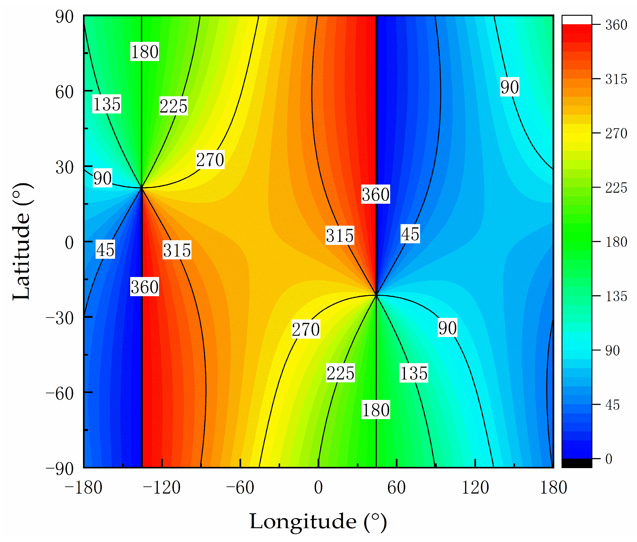
This study uses the time moment of 27 May 2024, UTC = 21 h, as a research sample. It has been found from the astronomical calendar that this time moment corresponds to the solar declination of δ = 21.4849° and E_ω = 0.0456 h. The contour color maps of the solar azimuth angle and solar altitude angle are shown in Figure 2 and Figure 3, respectively.

In Figure 2, the solar azimuth angle is defined as the angle between the line connecting the Earth’s true north point and the observation point and the line connecting the direct point of the sun and the observation point. The direct point of the sun refers to the point on the Earth’s surface where the sun’s rays are perpendicular; at this point, h_s is 90°. The line from the observation point to the true north point is taken as a reference direction (i.e., Y_n in the ENU coordinate system), where a clockwise direction indicates a positive direction. The value range of A_s is [0°, 360°], as indicated by the color bar on the right side of Figure 2. As shown in Figure 2, the contour lines representing the solar azimuth angle exhibit a ray-like pattern. It should be noted that Figure 2 depicts a projection of the three-dimensional spherical Earth onto a two-dimensional plane, which introduces certain distortion. Further, all contour lines intersect at the geographic poles where the latitude is either −90° or 90°, which indicates that at these locations, the azimuth angle can assume any value in the range of [0°, 360°]. Because of this distortion, in Figure 2, two geographic poles are illustrated as lines rather than points. This situation is very similar to a world map.

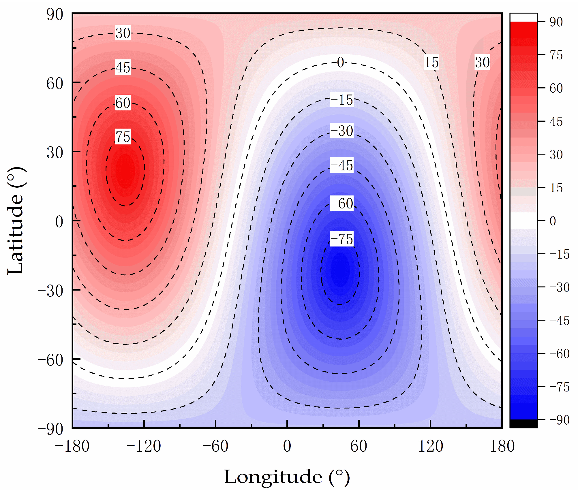
In Figure 3, the contour lines of the solar altitude angle radiate outward in concentric circles from the direct point of the sun, where the solar altitude angle is 90°, and the anti-direct point of the sun, which corresponds to the solar altitude angle of −90°.

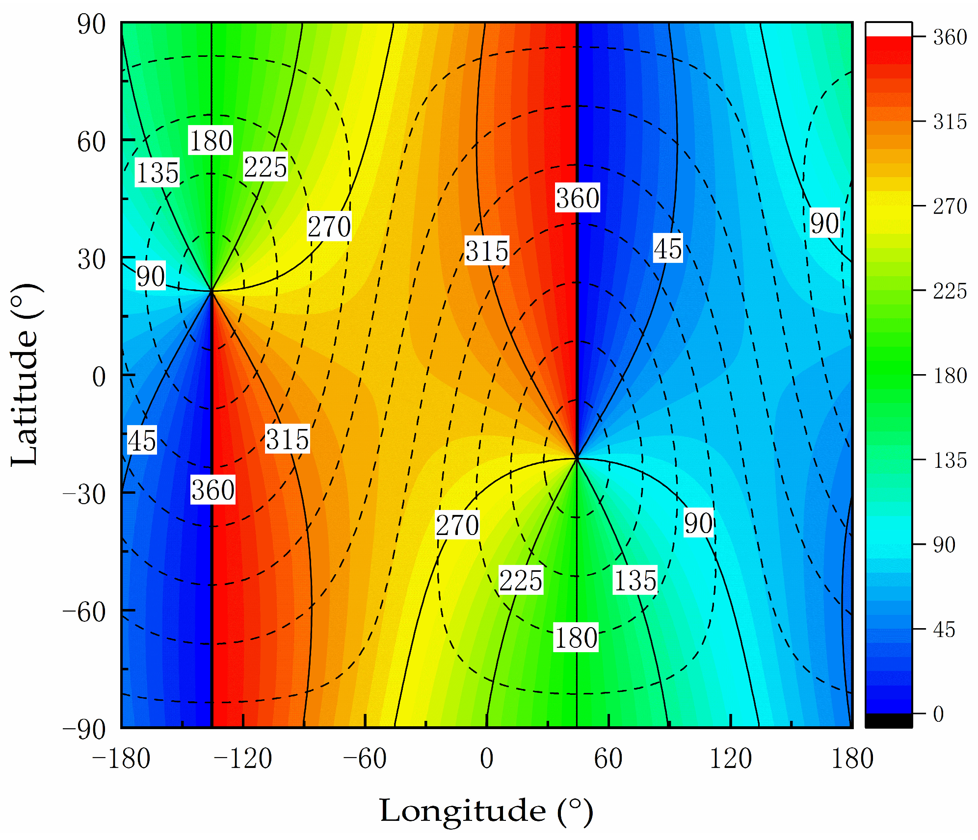
The color map presented in Figure 4 is constructed by superimposing the contour lines representing solar altitude angles in Figure 3 onto the contour lines in Figure 2. In Figure 4, the contour lines of h_s are denoted by the black dashed lines. In addition, to minimize clutter in the image annotations, Figure 4 displays only the contour line values corresponding to the azimuth angle, whereas the values for solar altitude angle are omitted. Thus, it can be inferred that the intersection points of the contour lines for solar azimuth angle and solar altitude angle indicate the solutions to the system of equations of the global positioning method. Analysis of Figure 4 reveals that most intersection points of the contour lines yield a single solution, whereas a minority present two solutions. The results of the analysis are consistent with the conclusions of the specific steps for solving the system of equations.

Figure 4 illustrates the number of solutions of the autonomous global positioning method at a designated time. The subsequent analysis focuses on the number of solutions to the equations of this method under different temporal conditions. As depicted in Figure 4, the distribution of the contour lines of the two independent variables determines the number of solutions to the equations. The distribution of the contour lines is mainly defined by the direct point of the sun, which is determined by the UTC. According to astronomy, during a 24 h period (i.e., one complete rotation of the Earth), the variations in a solar declination δ are very small. Therefore, the latitude of the direct point of the sun remains almost constant, whereas the longitude changes with time. For instance, when UTC changes from 21 h to 15 h, the superimposition of the contour lines of the two independent variables is highly similar to the graph obtained by shifting the map presented in Figure 4 horizontally along the horizontal axis by six hours; their global distribution of the number of solutions is also highly similar.

When looking at a yearly time frame, which represents one full orbit of the Earth around the sun, the changes in the solar declination become relatively apparent, requiring detailed examination. Astronomical data indicate that the solar declination varies throughout the year from −23°27′ to 23°27′. It is zero during the vernal and autumnal equinoxes and reaches its maximum and minimum values at the summer and winter solstices, respectively. 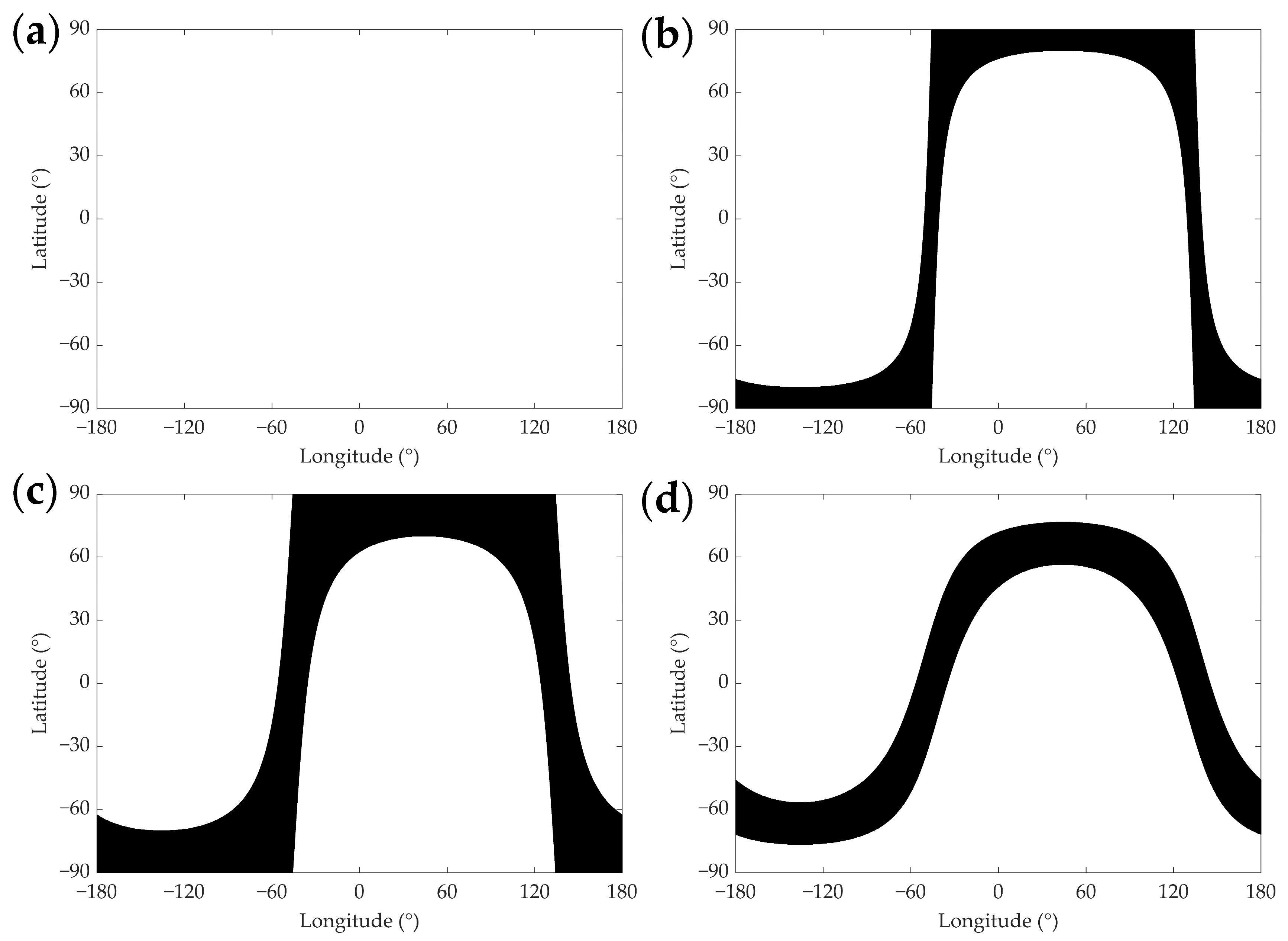Figure 5a–d show the global distribution of the number of solutions obtained by the autonomous global positioning method at the solar declinations of zero, 5°, 10°, and 23°27′ at the UTC of 21 h and E_ω = 169.8116/60/60 h, respectively.

In Figure 5, the white regions denote areas with a single solution, whereas the black regions indicate areas with two solutions. As shown in Figure 5a, when the solar declination is zero, there is only one global solution. In all other scenarios, there are areas with two solutions. It is important to understand that Figure 5 depicts the projection of the Earth’s three-dimensional spherical shape onto a two-dimensional surface, which can introduce certain distortion; thus, the visible size of the black regions in Figure 5 might not accurately reflect their actual surface area on the Earth.

3. Materials and Methods

This study presents the design of a global error model for the autonomous global positioning method. The main procedure of the model construction process involves the computation of partial derivatives of the system of equations composed of Equations (1) and (2). This system of equations represents an implicit function system that includes two independent variables: the solar azimuth angle (A_s) and the altitude angle (h_s). The two dependent variables are the longitude (η) and the latitude (ψ). This research aims to analyze the variations in the dependent variables caused by ΔA_s and Δh_s at different times and geographical locations. In addition, this study aims to evaluate actual geographical deviation (ΔL) associated with the changes in the two dependent variables. Consequently, the designed global error model enables a rapid estimation of the ΔL value based on the changes in the independent variables in practical applications.

First, the expressions for the four partial derivatives of the implicit function equation system are derived, and then the expression for the global positioning distance error (ΔL) is obtained.

Next, the conditions under which the error model is valid are studied, assuming that the implicit function equation system is differentiable during the derivation process of the positioning error expression. When this system is differentiable, the total differentials denote the best linear approximation of the total increments for small changes in A_s and h_s, that is, Δη ≈ dη and Δψ ≈ dψ. The findings of this study indicate that the error model is valid for specific geographical locations. However, for some geographical locations, the proposed model is demonstrated to be invalid.

3.1. Global Positioning Distance Error Expression Derivation

For the implicit function equation system, this study computes the partial derivatives with respect to the two independent variables: the solar azimuth angle (A_s) and the solar altitude angle (h_s). During the calculation process of partial derivatives, the solar declination (δ) is considered constant, resulting in four partial derivatives, which can be expressed as follows:

$$\begin{array}{l}{\displaystyle \frac{\partial \psi }{\partial A_{\mathrm{s}}}}=-{\displaystyle \frac{\sin A_{\mathrm{s}}\cos h_{\mathrm{s}}\cos \psi }{\cos A_{\mathrm{s}}\cos h_{\mathrm{s}}\sin \psi -\sin h_{\mathrm{s}}\cos \psi }},\\ {\displaystyle \frac{\partial \psi }{\partial h_{\mathrm{s}}}}=-{\displaystyle \frac{\sin h_{\mathrm{s}}\cos A_{\mathrm{s}}\cos \psi -\cos h_{\mathrm{s}}\sin \psi }{\cos A_{\mathrm{s}}\cos h_{\mathrm{s}}\sin \psi -\sin h_{\mathrm{s}}\cos \psi }},\\ {\displaystyle \frac{\partial \eta }{\partial A_{\mathrm{s}}}}=-{\displaystyle \frac{\cos A_{\mathrm{s}}\cos h_{\mathrm{s}}\cos \psi }{\sin h_{\mathrm{s}}-\sin \psi \sin \delta }},\\ {\displaystyle \frac{\partial \eta }{\partial h_{\mathrm{s}}}}={\displaystyle \frac{\sin A_{\mathrm{s}}\sin h_{\mathrm{s}}\cos \psi }{\sin h_{\mathrm{s}}-\sin \psi \sin \delta }}.\end{array}$$

(8)

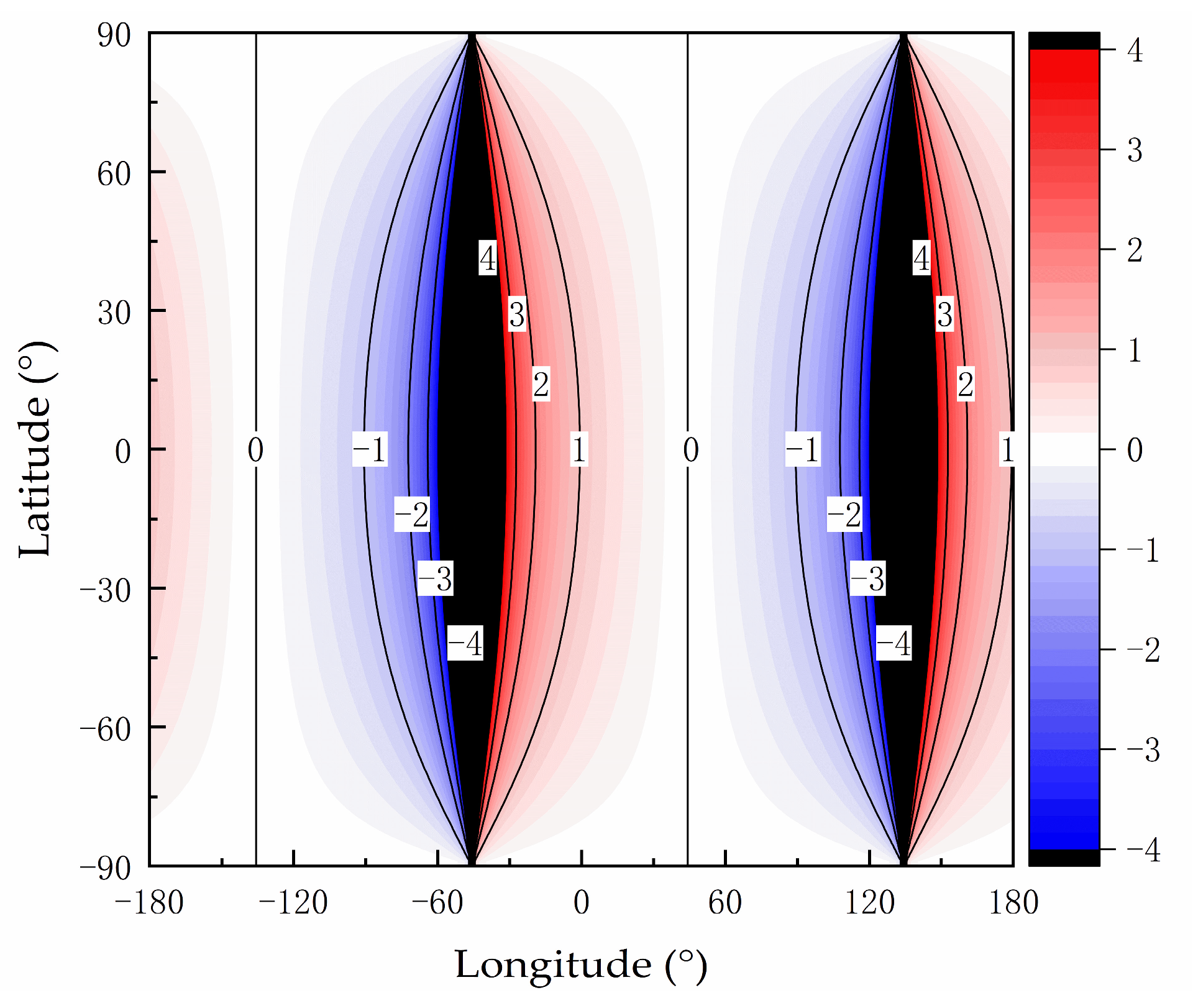
To ensure an initial understanding of the global distribution of partial derivatives, it is essential to further describe Equation (8) through visual representations. According to Equations (1), (2), and (8), the calculation equation of the partial derivative includes three variables: longitude (η), latitude (ψ), and time (UTC). Because a two-dimensional image can illustrate only the influence of two variables on a partial derivative, in this study, two-dimensional images are created by setting time to a specific value, using longitude as a horizontal axis and latitude as a vertical axis to illustrate the global distribution of partial derivatives.

The specific calculation steps of a partial derivative ∂ψ/∂A_s are as follows:

• Define ƒ (η, ψ, UTC) = ∂ψ/∂A_s, where η, ψ, and UTC are the three calculation variables. Set the time to be consistent with the time in Figure 2, which is 27 May 2024, UTC = 21 h. At this time, δ = 21.4849° and E_ω = 0.0456 h. Consequently, express ƒ (η, ψ, 21) = ∂ψ/∂A_s.
• Calculate the value of a function ƒ (η, ψ, 21) using the two independent variables, namely η and ψ. The value range of the Earth’s latitude (ψ) is [−90°, 90°], with an interval of 0.01°, resulting in a total of 18,000 data points. The value range of the Earth’s longitude (η) is [−180°, 180°], also with an interval of 0.01°, resulting in 36,000 data points. Therefore, the total number of calculations amounts to 648,000,000. For each calculation, first, the values of solar altitude angle (h_s) and azimuth angle (A_s) are calculated for each geographical location using Equations (1) and (2). Next, the values of the solar declination, geographical latitude, solar altitude angle, and solar azimuth angle of each geographical location are substituted into Equation (8) to calculate the partial derivative ƒ (η, ψ, 21) value.

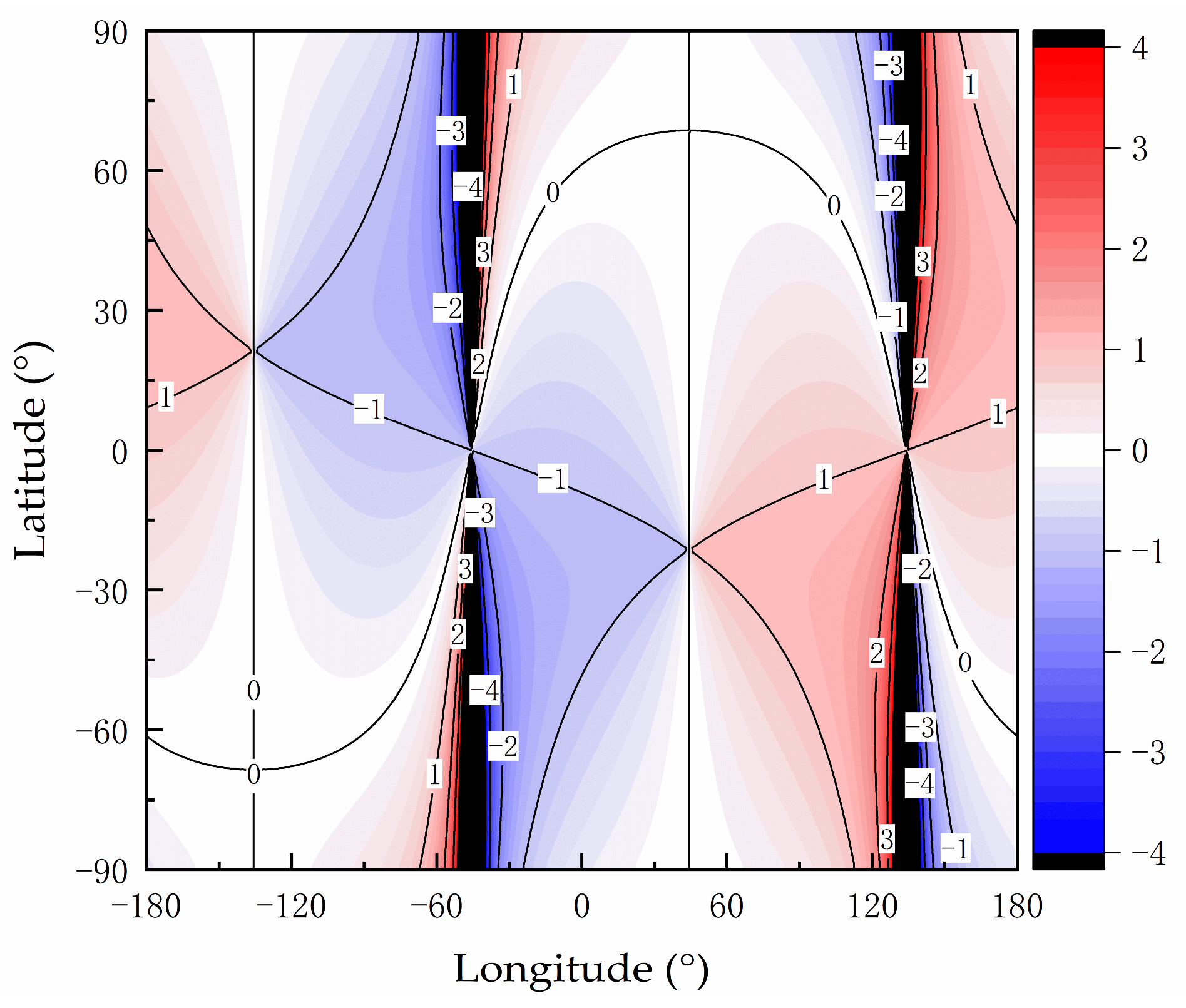
In summary, the global distribution of a partial derivative (∂ψ/∂A_s) at the UTC of 21:00 on 27 May 2024 is obtained, as illustrated in Figure 6. The simulation calculations were performed using MATLAB software, R2023a (9.14.0.2206163), 22 February 2023. In Figure 6, the horizontal axis represents longitude, and the vertical axis indicates the latitude value. The contour lines represent the values of the partial derivative of the latitude angle with respect to the solar azimuth angle. The calculations of the remaining partial derivatives are performed in the same manner as that of ∂ψ/∂A_s, as shown in Figure 7, Figure 8 and Figure 9.

However, in Figure 6, Figure 7, Figure 8 and Figure 9, considering the drastic changes in the partial derivatives’ values at certain locations, areas where the absolute value exceeds four are illustrated in black. This approach is employed to ensure that most regions can accurately show the values of the four partial derivatives.

Further, assuming that the implicit function equations are differentiable at all locations globally, the total differential (dψ) can be regarded as a total increment (Δψ), and the same rule will apply to the longitude. The total increments of longitude and latitude can be mathematically expressed as follows:

$$\begin{array}{l}\Delta \psi \approx \mathrm{d}\psi ={\displaystyle \frac{\partial \psi }{\partial A_{\mathrm{s}}}}\Delta A_{\mathrm{s}}+{\displaystyle \frac{\partial \psi }{\partial h_{\mathrm{s}}}}\Delta h_{\mathrm{s}},\\ \Delta \eta \approx \mathrm{d}\eta ={\displaystyle \frac{\partial \eta }{\partial A_{\mathrm{s}}}}\Delta A_{\mathrm{s}}+{\displaystyle \frac{\partial \eta }{\partial h_{\mathrm{s}}}}\Delta h_{\mathrm{s}}.\end{array}$$

(9)

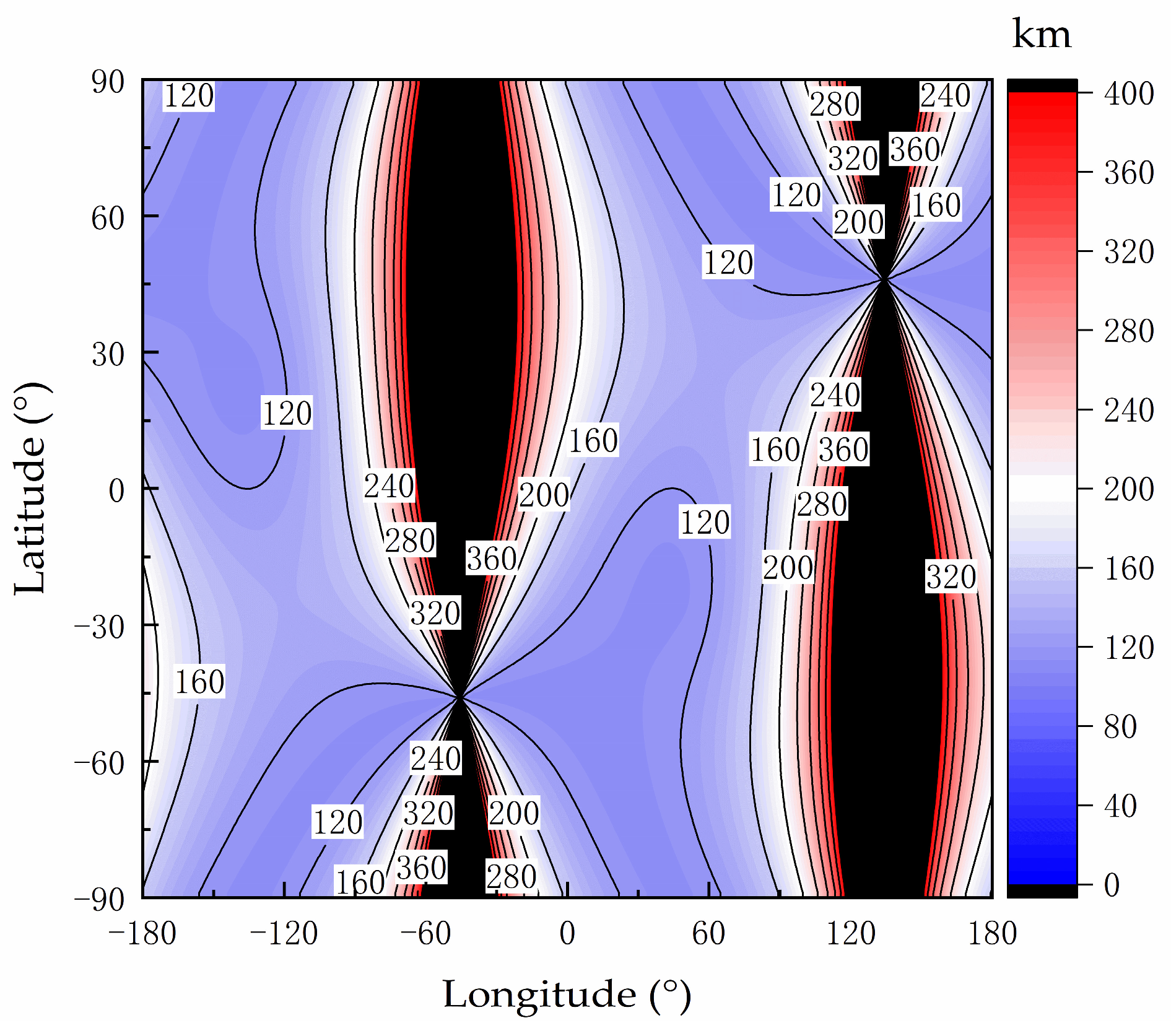
However, total increments of longitude and latitude do not represent the final positioning distance error (ΔL). If the measured longitude and latitude values at a point (η, ψ) on the Earth’s surface are (η + Δη, ψ + Δψ), the measurement deviations of the two independent variables will be ΔA_s and Δh_s, respectively. In addition, assuming that the Earth’s surface is a standard sphere, the spherical distance between the two points can be calculated as follows:

$$\Delta L=\arccos (\cos (\psi )\times \cos (\psi +\Delta \psi )\times \cos (\Delta \eta )+\sin (\psi )\times \sin (\psi +\Delta \psi ))\times R_{\mathrm{L}},$$

(10)

where R_L is the Earth’s radius, and is set to 6400 km in this study.

Therefore, the global positioning distance error calculated by the proposed error model is obtained by:

$$\mathrm{d}L=\arccos (\cos (\psi )\times \cos (\psi +\mathrm{d}\psi )\times \cos (\mathrm{d}\eta )+\sin (\psi )\times \sin (\psi +\mathrm{d}\psi ))\times R_{\mathrm{L}}.$$

(11)

In conclusion, the proposed error model is defined by Equations (8), (9), and (11). This model enables the calculation of positioning distance errors of the autonomous global positioning method for any longitude and latitude values on the Earth’s surface.

3.2. Conditions Under Which the Proposed Error Model Is Valid

The accurate assessment of the validity of the proposed error model at a particular geographic location examines whether the four partial derivatives of the two dependent variables, derived from the system of two implicit functions, exist and exhibit continuity at that specific point. The main mathematical symbols employed in Section 3.2 are presented in

Table 1. The main mathematical symbols in Section 3.2.

ψ ∈ Uψ	η ∈ Uη	N	cos ψ	M
ψN≠0 ∈ Cψ	ηN≠0 ∈ Cη	≠0	≠0	≠0
ψN=0 ∈ Aψ	ηN=0 ∈ Aη	0	---	---

.

The determination process of a function’s differentiability is complex. By analyzing the properties of the four partial derivatives, this study determines whether this process can be simplified. The four partial derivatives consist of elementary functions, which are derived from the sum, difference, product, and quotient of trigonometric functions. Consequently, the four partial derivatives are classified as elementary functions. Further, according to the mathematical principles, elementary functions are continuous and differentiable at every point within their domain. Thus, determining whether the proposed error model is differentiable at a specific point on the Earth’s surface (η, ψ) can be reduced to the process of verifying whether the four partial derivatives are defined at that point. If all four partial derivatives are defined at a given point, then the error model is considered differentiable at that point. However, if any one of the four partial derivatives is undefined at a particular point, the model is regarded as non-differentiable at that point.

To examine whether an elementary function is defined at a specific point, it is necessary to distinguish the type of elementary function. The function types include fractional forms, radical forms, and logarithmic forms, among others. The four partial derivatives are expressed in fractional form, so they are defined where the denominator is not equal to zero.

In summary, when the denominators of the four partial derivatives are all non-zero, the derivatives are simultaneously defined at a specific point. In addition, as all these functions are elementary functions, they exist and are continuous at that point. Consequently, at that point, the implicit function system is differentiable, and the total differential can be considered the total increment, indicating that the error model is valid at the given point. In contrast, if any one of the four partial derivatives has a denominator that equals zero, the implicit function system is not differentiable at the given point, and the proposed error model is inapplicable at that point.

Next, the denominators of the four partial derivatives are studied. According to Equation (8), the denominators of partial derivatives ∂ψ/∂A_s and ∂ψ/∂h_s are equal, and the denominators of partial derivatives ∂η/∂A_s and ∂η/∂h_s are also equal. The two denominators are expressed as follows:

$$\begin{array}{l}M=\cos A_{\mathrm{s}}\cos h_{\mathrm{s}}\sin \psi -\sin h_{\mathrm{s}}\cos \psi ,\\ N=\sin h_{\mathrm{s}}-\sin \psi \sin \delta .\end{array}$$

(12)

Combining Equations (1), (2), and (12), the relation between N and M is expressed as follows:

$$N=-\cos (\psi )M.$$

(13)

3.2.1. Denominator N Equals Zero

First, the case when the denominator N of a partial derivative equals zero is examined. By considering UTC a constant and treating longitude and latitude as two independent variables for further analysis, the following expression can be obtained:

$$g\left({\eta }_{N=0},{\psi }_{N=0}\right)=N=0.$$

(14)

According to the definition of longitude, the value range of η is from −180° to 180°. The set of all longitude (η) values is defined as U_η, and the set of all η values, where N = 0, is denoted as A_η; set A_η denotes a subset of U_η. Next, let set A_η be a universal set; then, the complement of A_η is C_η. Similarly, according to the definition of latitude, the value range of ψ is from −90° to 90°. The set of all latitude (ψ) values is denoted by U_ψ, and the set of all ψ where N = 0 is labeled as A_ψ and represents a subset of U_ψ. Further, let set U_ψ be a universal set; then, the complement of A_ψ is C_ψ. A summary of the set labels is provided in Table 1.

Based on the latitude (ψ) value, there are two possible cases: (1) ψ equals 90° or −90°, and (2) ψ is in the interval (−90°, 90°).

When ψ equals 90° or −90°, cos ψ = 0, as shown in row 2 of

Table 2. Two possible cases based on the latitude value.

ψN=0	ηN=0	N	cos ψ	M
90° or −90°	[−180°, 180°]	0	0	any
(−90°, 90°)	ηN=0,cos ω=0	0	≠0	0

. According to Equation (13), regardless of the denominator (M) value, the denominator (N) is equal to zero. The (η_N=0,ψ_N=0) set of row 2 in Table 2 corresponds to the geographic locations of the South and North Poles. Every meridian passes through both the South and North Poles; the latitude of the South Pole is −90°, and its longitude can be any value from the [−180°, 180°] range. The latitude of the North Pole is 90°, and its longitude can also be any value from the [−180°, 180°] range.

When ψ is in the (−90°, 90°) interval, cos ψ ≠ 0, as shown in row 3 of Table 2. Further, since N is zero, according to Equation (13), M is also zero. Substituting Equations (2) and (12) into Equation (14) yields

$$\cos \psi \cos \delta \cos \omega =0.$$

(15)

Because the value range of solar declination (δ) is [−23°27′, 23°27′], then cosδ ≠ 0; therefore, cosω = 0. Combining this with Equation (2) yields

$${\eta }_{N=0,\cos \omega =0}=\left\{\begin{array}{c}270°-(UT\mathrm{C}+E_{\mathsf{\omega }})\times 15°, \omega =90°, \\ 450°-(UT\mathrm{C}+E_{\mathsf{\omega }})\times 15°, \omega =270°,\end{array}\right.$$

(16)

where the latitude (ψ_N=0) value is in the (−90°, 90°) range.

By combining the two above-presented conclusions, it can be found that (η_N=0,ψ_N=0) satisfies Equation (14), as shown in Table 2. In other words, sets A_η and A_ψ are obtained as shown in row 3 of Table 1. The three-dimensional spatial distribution of sets A_η and A_ψ forms a circular ring, which consists of two lines of longitude on Earth. At this ring, the denominator of the partial derivative (N) is zero, and the implicit function system is non-differentiable. Consequently, the proposed error model is invalid at (η_N=0,ψ_N=0).

3.2.2. Denominator N Differs from Zero

Next, the case where the denominator of the partial derivative (N) differs from zero is analyzed, as shown in row 2 of Table 1. In this case, it holds that

$$g\left({\eta }_{N\ne 0},{\psi }_{N\ne 0}\right)=N\ne 0,$$

(17)

Based on Equation (13), it follows that cos ψ ≠ 0; thus, ψ_N≠0 is in the interval (−90°, 90°). Next, according to Equation (13), the denominator M of the partial derivative differs from zero, indicating that the denominators of the four partial derivatives are non-zero. Through a proof by contradiction, it can be proven that all elements ψ_N≠0 that satisfy Equation (17) belong to set C_η, which is defined as a complement set of set A_η. Similarly, all ψ_N≠0 that satisfy Equation (17) are in a complement set C_ψ of set A_ψ.

The specific proof is as follows. All longitudes belong to universal set U_η. Sets A_η and C_η are both subsets of set U_η, and set C_η is a complement set of set A_η. If an element η_N≠0 does not belong to set C_η, then element η_N≠0 belongs to set A_η. Further, it can be concluded that N = 0, which contradicts N ≠ 0. Therefore, all elements η_N≠0 that satisfy Equation (17) are in the complement set C_η. Similarly, the corresponding conclusion can be drawn for latitudes.

3.2.3. Conditions Summary

In summary, the proposed error model is differentiable at points (η_N≠0, ψ_N≠0) where the denominators of the four partial derivatives are simultaneously non-zero, as shown in row 2 of Table 1. Within the circular ring defined by sets A_η and A_ψ, as presented in Section 3.2.1, the error model is not differentiable, meaning it is not valid in this case. According to Equation (16), the circular ring is determined by the UTC and E_ω, and is independent of the solar declination.

4. Global Error Model Verification by Numerical Simulations

The correctness and accuracy of the global positioning error (dL) calculated by the proposed error model were verified by numerical simulations. When the error model was valid, the total increment of the positioning error was approximately equal to the total differential (ΔL ≈ dL).

According to the foundational principles of calculus, when the change in the independent variable was small, the total increment could be effectively approximated by the total differential. This study showed that when the absolute value of the measurement deviation was less than or equal to 5° (|ΔA_s| ≤ 5°, |Δh_s| ≤ 5°), the total increment could be approximated as a total differential. Under these specified conditions, the error model established in Section 3 was validated.

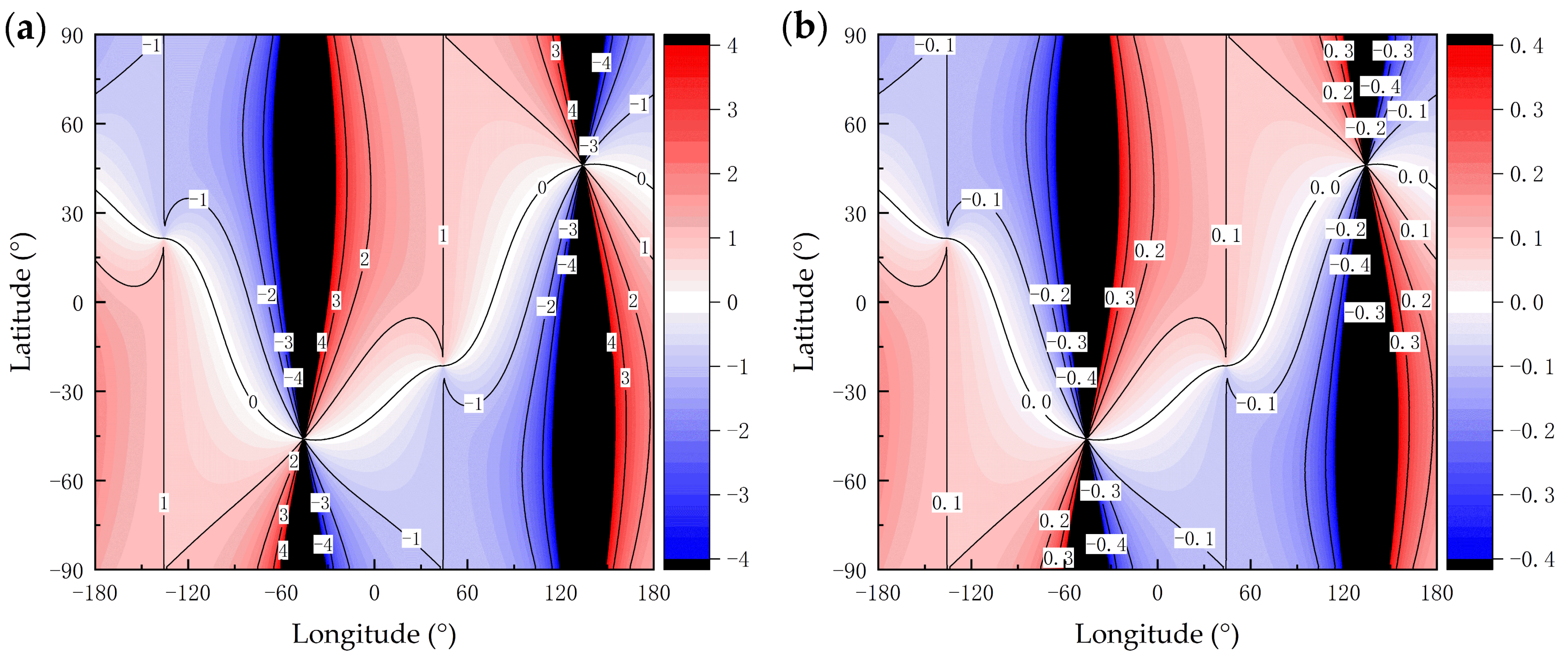
The presence of multiple variables in Equation (9) could make an effective representation of analysis results using a single two-dimensional graph challenging. Therefore, this study employed a case-by-case discussion to reduce the number of variables, thus facilitating a clearer presentation of the results. The discussion was conducted for two distinct cases: ΔA_s = Δh_s and ΔA_s ≠ Δh_s. The simulation calculations were performed using MATLAB (Matrix laboratory) software.

4.1. First Case Analysis: ΔA_s Equals Δh_s

In this simulation experiment, first, ΔA_s = Δh_s was substituted into Equation (9), which yielded

$${\displaystyle \frac{\mathrm{d}\psi }{\Delta A_{\mathrm{s}}}}={\displaystyle \frac{\partial \psi }{\partial A_{\mathrm{s}}}}+{\displaystyle \frac{\partial \psi }{\partial h_{\mathrm{s}}}},$$

(18)

$${\displaystyle \frac{\mathrm{d}\eta }{\Delta A_{\mathrm{s}}}}={\displaystyle \frac{\partial \eta }{\partial A_{\mathrm{s}}}}+{\displaystyle \frac{\partial \eta }{\partial h_{\mathrm{s}}}},$$

(19)

where dψ/ΔA_s is the total differential ratio of the latitude to the solar azimuth angle (TDRLAT), and dη/ΔA_s is the total differential ratio of the longitude to the solar azimuth angle (TDRLON). It should be noted that neither TDRLAT nor TDRLON are a partial derivative or a total differential, but were introduced in this study for the convenience of graphical representation of the error analysis results.

Considering the same conditions as those in Figure 6, Figure 7, Figure 8 and Figure 9, the TDRLAT and TDRLON obtained in this experiment are shown in Figure 10a and Figure 11a, respectively. These conditions are UTC = 21 h, δ = 21.4849°, and E_ω = 0.0456 h.

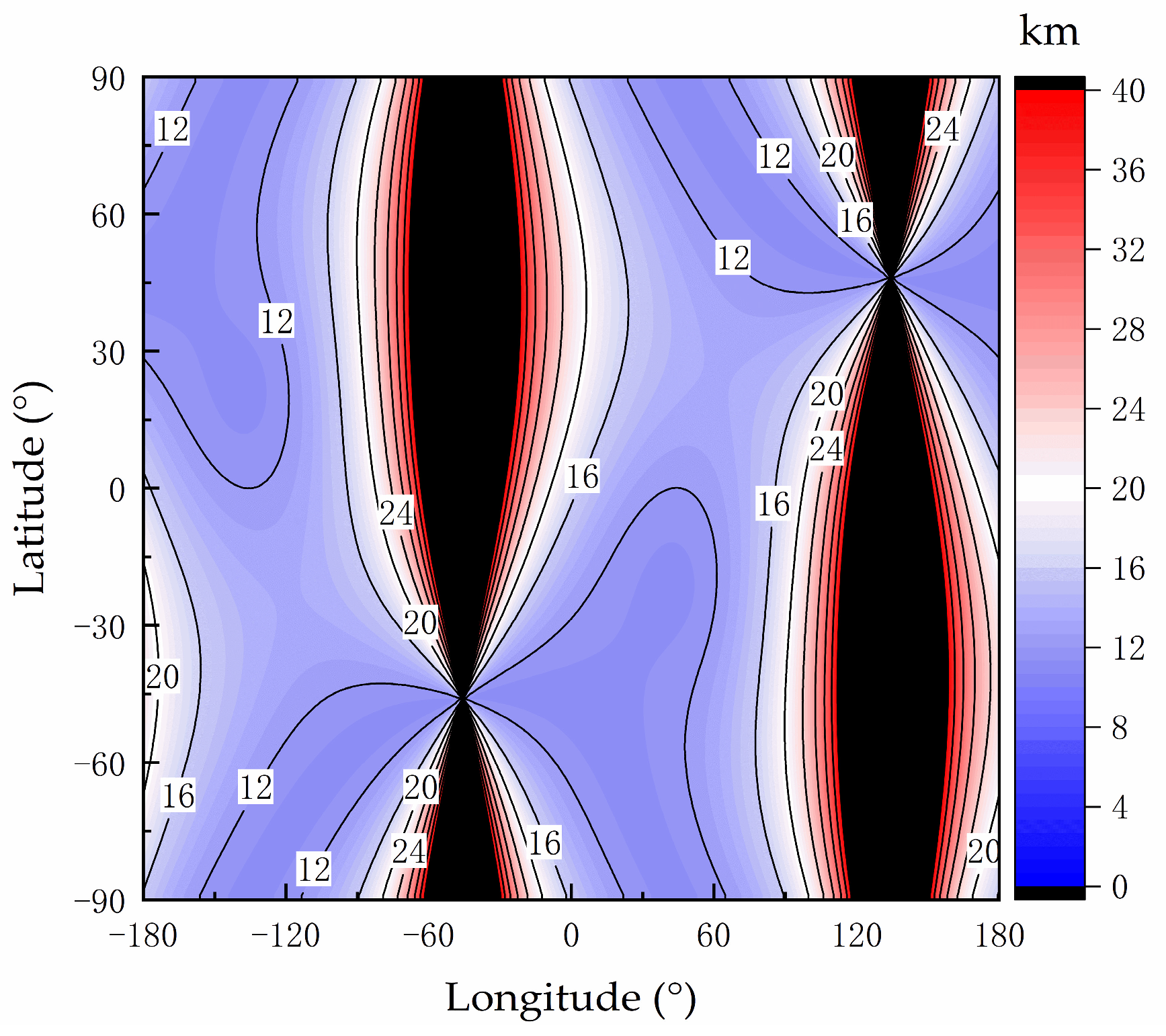
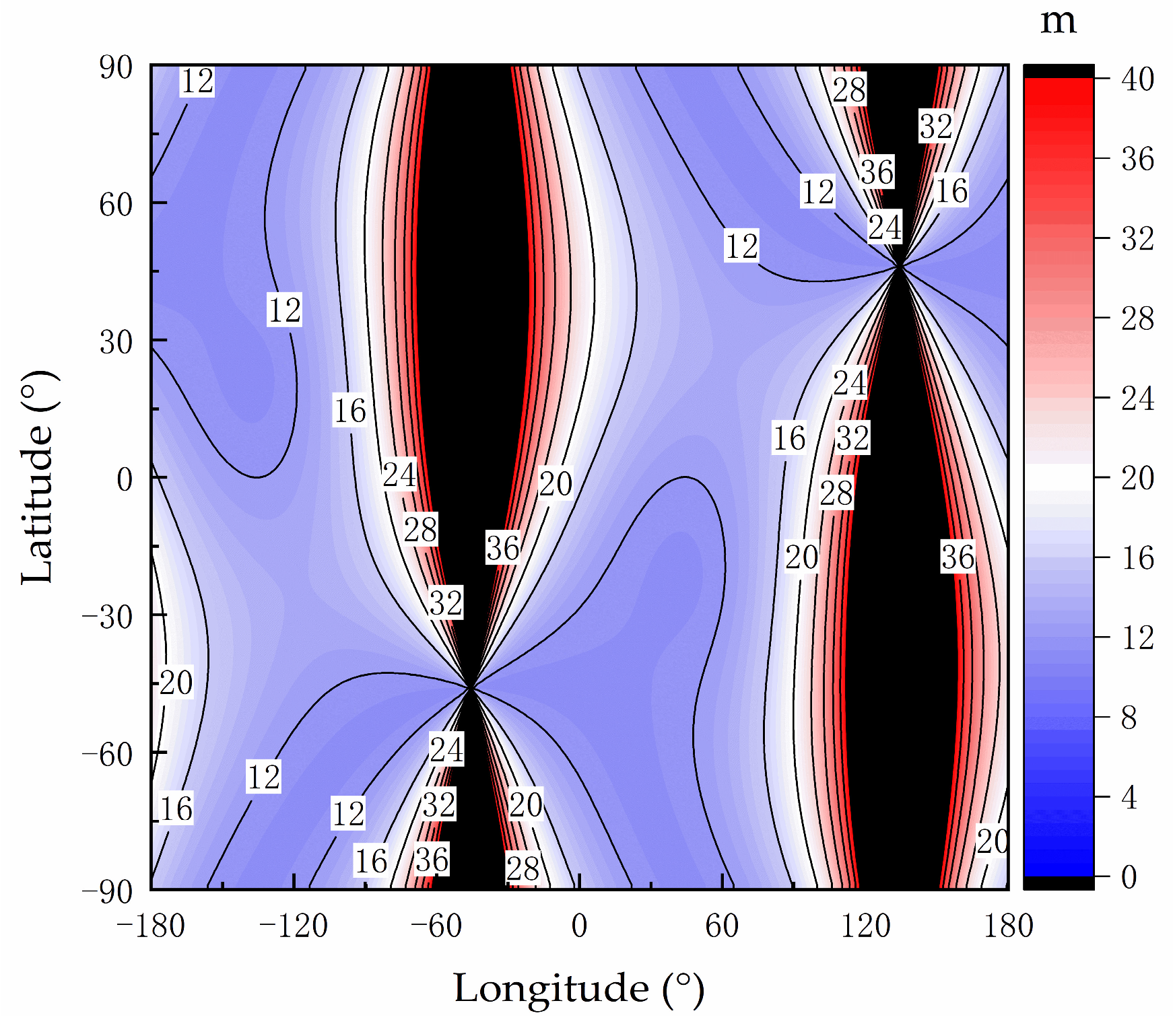
For ΔA_s = Δh_s = 0.1°, the global distribution map of the total latitude increment Δψ was obtained, as shown in Figure 10b; the global distribution map of the total longitude increment Δη is displayed in Figure 11b.

The calculation process was as follows. First, it was assumed that the theoretical solar altitude angle and azimuth angle at a point on Earth (η, ψ) were A_s and h_s, and their measurement deviations were ΔA_s and Δh_s, respectively; UTC = 21 h, δ = 21.4849°, and E_ω = 0.0456 h. Then, the measured solar altitude angle and azimuth angle at point (η, ψ) were obtained as (A_s + ΔA_s) and (h_s + Δh_s). By substituting the measured solar altitude angle and azimuth angle into Equations (1) and (2), the measured latitude and longitude $\left({\eta }^{\prime },{\psi }^{\prime }\right)$ values were obtained. If the system of equations, composed of Equations (1) and (2), had two sets of solutions, the solution that was closer to the theoretical solution was considered a unique solution, whereas the other solution was excluded. Then, it held that $\Delta \psi ={\psi }^{\prime }-\psi$ and $\Delta \eta ={\eta }^{\prime }-\eta$.

In Figure 10a and Figure 11a, in the numerical bar on the right side, the values exhibiting an absolute total differential ratio larger than four (dimensionless) are depicted in black. In Figure 10b and Figure 11b, regions where the absolute values of latitude and longitude deviations surpassed 0.4° are also illustrated in black. In Figure 10a,b and Figure 11a,b, all other areas are represented in color.

Therefore, Figure 10 and Figure 11 depict two distinct regions, namely the colored and black regions, each of which was analyzed independently, as presented in the following sections.

4.1.1. Colored Region

The results presented in Figure 10a were calculated by Equation (18); Figure 10b shows latitude deviation Δψ for all global locations when ΔA_s = Δh_s = 0.1°. In Figure 10a, all points on the contour line labeled as “1” had dψ/ΔA_s = 1. In Figure 10b, all points on the contour line labeled as “0.1” had Δψ = 0.1°, which yielded Δψ/ΔA_s = 1.

The colored areas in Figure 10a,b indicate that the contour line distribution patterns displayed in these figures were consistent, meaning that dψ/ΔA_s ≈ Δψ/ΔA_s. Consequently, it could be determined that Δψ ≈ dψ.

The contour line distribution patterns presented in Figure 11a,b were also consistent, indicating that Δη ≈ dη.

Further research indicated that when ΔA_s = Δh_s ≠ 0.1°, for example, ΔA_s = Δh_s = 0.5° or ΔA_s = Δh_s = 3°, the global error model remained valid in the colored region.

4.1.2. Black Region

First, the black areas in Figure 10a and Figure 11a contained the region where the proposed error model was not valid. As noted in Section 3.2, the region where the error model was not valid was a circular ring. In Figure 10 and Figure 11, the time was 27 May 2024, UTC = 21 h, and E_ω = 169.8116/60/60 h. According to Equation (16), the η_{N=0,cos ω=0} value was either −45.7° or 134.3°. The black areas in Figure 10a and Figure 11a are distributed around the circular ring defined by the longitude value, η_{N=0,cos ω=0}. Therefore, the black areas contained the region where the proposed error model was invalid.

Then, in Figure 10 and Figure 11, the areas in black, excluding the circular ring, were examined; these black areas outside the circular ring were called the valid black areas. In Figure 10a and Figure 11a, the valid black area was characterized by a gradual increase in the absolute value of the ratio of total differentials of latitude and longitude (i.e., the TDRLON and TDRLAT values), ranging from four to positive infinity. By zooming in on this area, it was observed that the contour line distribution patterns in Figure 10a,b were consistent, as well as those in Figure 11a,b, meaning that the distribution pattern of total increments was consistent with the distribution pattern of total differential ratios. Consequently, it could be inferred that the error model remained applicable within the valid black area. Nevertheless, it should be noted that due to the excessively high absolute value of the total differential ratio (the TDRLON and TDRLAT values), even minimal measurement errors in the independent variables could cause significant deviations in latitude and longitude.

Further research indicated that when ΔA_s = Δh_s ≠ 0.1°, for instance, or ΔA_s = Δh_s = 0.5° or ΔA_s = Δh_s = 3°, the conclusions regarding the valid black areas and the invalid circular ring still held true.

4.2. Second Case Analysis: ΔA_s Differs from Δh_s

This case analyzed the situation when ΔA_s ≠ Δh_s. This case could include many possibilities, such as ΔA_s = −2 × Δh_s, ΔA_s = 5 × Δh_s, and ΔA_s = −Δh_s.

This study selected cases of ΔA_s = −2 × Δh_s, ΔA_s = 0.2°, and Δh_s = −0.1° for the analysis, and two global distribution maps were obtained by the calculation process described in Section 4.1, as shown in Figure 12 and Figure 13. Similar to Figure 10 and Figure 11, Figure 12a and Figure 13a display the total differential ratios, and Figure 12b and Figure 13b depict the total increments. After analysis, it was concluded that the results obtained in the colored and black areas in Section 4.1 still held true. In Figure 12 and Figure 13, the global error model remained valid in the colored region; the black areas contained the region where the proposed error model was invalid; and the error model remained applicable within the valid black area.

Finally, when the ratio of ΔA_s to Δh_s is other value, the same conclusions for both the colored region and the black region could be drawn.

4.3. Summary

The results presented in Section 4.1 and Section 4.2 demonstrate that when the absolute value of the measurement deviation was less than 5° (|ΔA_s| ≤ 5°, |Δh_s| ≤ 5°), the proposed error model’s accuracy was validated. This also confirmed the correctness of the conditions under which the proposed error model was valid.

Conversely, when the absolute value of the measurement deviation exceeded 5° (|ΔA_s| > 5°, |Δh_s| > 5°), the proposed error model’s accuracy decreased.

5. Results

This research aimed to evaluate the actual geographical deviation (ΔL) caused by ΔA_s and Δh_s values at different times and locations. When the time was fixed, the distribution pattern of ΔL at different geographical locations worldwide was referred to as the spatial properties of the proposed error model. When time changed, the distribution pattern of ΔL at the same location was referred to as the temporal properties of the proposed error model. The calculations were performed using MATLAB software. The research results of the two types of properties are presented in the following sections.

5.1. Error Model Spatial Properties

During the computational process, the ΔA_s and Δh_s values were both expressed in degrees (°), and the ΔL value was quantified in kilometers (km). At the time of 27 May 2024, UTC = 21 h, based on the UTC and the astronomical calendar, δ = 21.4849°, and E_ω = 0.0456 h. Subsequently, the four partial derivatives of all positions on the Earth’s surface were calculated according to Equations (1), (2), and (8).

When the measurement biases of the independent variables were ΔA_s = Δh_s = 1°, ΔA_s = Δh_s = 0.1°, and ΔA_s = Δh_s = 0.0001°, all ΔA_s and Δh_s satisfied the condition in Section 4.3 that |ΔA_s| ≤ 5° and |Δh_s| ≤ 5°. Consequently, the proposed error model was valid for most global locations under these conditions. It could be inferred that Δη was approximately equal to dη and Δψ was approximately equal to dψ. The corresponding dψ and dη values were obtained by Equation (9). Subsequently, the corresponding positioning errors (ΔL) were calculated using Equation (11), as illustrated in Figure 14, Figure 15 and Figure 16. Because Equation (11) was used instead of Equation (10), the calculation time was significantly decreased. This reduction in time is the main contribution of the proposed error model.

In Figure 14, the horizontal axis represents longitude, and the vertical axis indicates the latitude value. The contour lines represent the values of the positioning error. Most contour lines intersect at two points, both of which are on the invalid circular ring mentioned in Section 3.2.3. The results indicate that the positioning error in most regions was within 140 km. The black area in Figure 14 indicates an error larger than 400 km, with the central points exhibiting errors of positive infinity. This black area could be divided into two parts, as mentioned in Section 4.1.2: the region where the proposed error model was not valid and the region where the partial derivatives gradually approached positive infinity. The former region is a circular ring; the latter region is referred to as the valid black area.

When ΔA_s = Δh_s = 0.1°, the global positioning error ΔL was generally within 14 km, as shown in Figure 15.

When ΔA_s = Δh_s = 0.0001°, as shown in Figure 16, the distribution pattern of ΔL remained the same as that shown in Figure 15, with the global positioning error mostly within 14 m. The positioning accuracy of GPS typically falls within the meter range. Therefore, if an autonomous global positioning system using the Earth’s sky polarized light and true north measurement instruments can achieve performance comparable to that of the GPS, the accuracy of the polarized light sensors should be 0.0001°.

5.2. Error Model Temporal Properties

When the time changed, for instance, when the time was 27 May 2024, UTC = 15 h. Based on the UTC and the astronomical calendar, δ = 21.4443° and E_ω = 0.0461 h. The computational process in Section 5.1 was employed to calculate the global error distribution for ΔA_s = Δh_s = 0.1°, as displayed in Figure 17. The global distribution did not change but shifted parallel along the horizontal axis.

6. Discussion

Based on the proposed error model, the geographical deviation (ΔL) can be rapidly and accurately calculated. Figure 14, Figure 15, Figure 16 and Figure 17 illustrate the global distribution patterns of ΔL at different times. The patterns are non-linear. The black regions in Figure 14, Figure 15, Figure 16 and Figure 17 should be avoided, because even minor ΔA_s and Δh_s values could lead to significant positioning deviations ΔL at the specific time and location. Consequently, it is recommended to reconsider the navigation task to avoid such times and geographical locations.

The GPS’s positioning accuracy generally falls within the meter range. If an autonomous global positioning system using the Earth’s sky polarized light and true north measurement instruments can achieve performance comparable to that of the GPS, it is imperative to enhance the accuracy of the polarized light sensors. However, the review [13] indicates that the accuracy of these sensors typically ranges from 0.05° to 0.5°, which limits their capability of providing global positioning accuracy within the kilometer range.

There are several limitations to the practical implementation of the proposed model. Its application may be difficult for ordinary developers. It requires a high level of precision in input data. To achieve accuracy comparable to GPS (up to 14 m), too-small deviations of input angles (up to 0.0001°) are required. The model’s accuracy diminishes when measurement deviations exceed 5°, which can be a problem when used in dynamic environments.

7. Conclusions

The error model for the real-time global positioning method using the Earth’s sky polarized light and true north measurement instruments is developed. The proposed model can rapidly and accurately provide the global distribution patterns of positioning errors at different times and under different error conditions. The simulation results indicate that when the deviations of the two independent variables are up to 0.0001°, the positioning error mostly remains less than 14 m; the global distribution of the positioning errors are non-linear. In addition, the conditions under which the proposed error model is valid have been outlined. At a specific time, the error model is globally valid except for the circular ring, which is determined by the UTC and E_ω.