4.1. Segmentation Mask Evaluation
The test set results, summarized in
Table 4, provide a comparison of four encoder–decoder-based architectures (U-Net [
10], DeepLabv3+ [
9], FPN [
11], and Segformer [
8]), each paired with different encoder backbones—MobileNetV4, EfficientNet-B2, and ResNet-34. Results are grouped into Loss and Accuracy Metrics. The objective of the comparison is to assess each model and encoder combination on its semantic segmentation quality.
Across all evaluated architectures, EfficientNet-B2 consistently outperformed the other encoders, achieving higher overlap-based metrics such as Dice and IoU with low overall loss. For example, U-Net with EfficientNet-B2 attained a Dice score of 0.8392, an IoU of 0.6555, a test loss of 0.3608, a focal loss of 0.0240, and an F1-score of 0.7050. Similar improvements were observed for DeepLabv3+ and FPN when using the same encoder, confirming its reliability across different model architectures. The SegFormer architecture, when combined with EfficientNet-B2, delivered accuracy comparable to traditional CNN-based models such as FPN and DeepLabv3+, achieving a Dice score of 0.8376 and an IoU of 0.6459. In contrast, all models using MobileNetV4 consistently underperformed in accuracy metrics. For instance, U-Net with MobileNetV4 reached only 0.7919 Dice, 0.6014 IoU, and had the highest test loss.
When evaluated on downsampled images of 480 × 304 pixels (
Table 5), the U-Net with a ResNet-34 encoder achieves the highest overlap metrics Dice score of 0.7766 and IoU of 0.6193, outperforming DeepLabv3+ with EfficientNet-B2 Dice score of 0.7554 and IoU of 0.6012.
Both U-Net (ResNet-34) and DeepLabv3+ (EfficientNet-B2) trained on SAM2-generated masks underperform compared to using SegFormer-B5-derived labels. For instance, U-Net’s Dice (0.6913) and IoU (0.5543) are roughly 15 points lower than with SegFormer-B5 masks. This semantic gap arises because SAM2’s class-agnostic approach lacks explicit category guidance; its masks may group adjacent regions without regard for class boundaries, whereas SegFormer-B5, pre-trained on Cityscapes, produces semantically coherent outlines aligned with object classes. Consequently, downstream models learn from noisier, semantically ambiguous labels with SAM2, leading to degraded segmentation performance seen in
Table 6.
In our study, to better approximate real-world conditions and the robustness of the models, we included test scenarios that simulate partial information loss due to adverse weather, such as rain, as well as interference during data transmission leading to packet-loss artifacts. We applied
transforms.RandomErasing (
, scale
, ratio
) on test set to replace 2–33% of each image with random noise. Under this corruption (
Table 7), U-Net (ResNet-34) total loss increases from 0.355 to 0.844 and Dice drops from 0.845 to 0.776, while DeepLabv3+ (EfficientNet-B2) total loss rises from 0.330 to 0.699 and Dice from 0.838 to 0.765, indicating slightly better resilience of DeepLabv3+. Moreover, these results indicate that, even under partial information loss during inference, the evaluated models maintain basic stability.
4.2. Computational Requirements Comparison
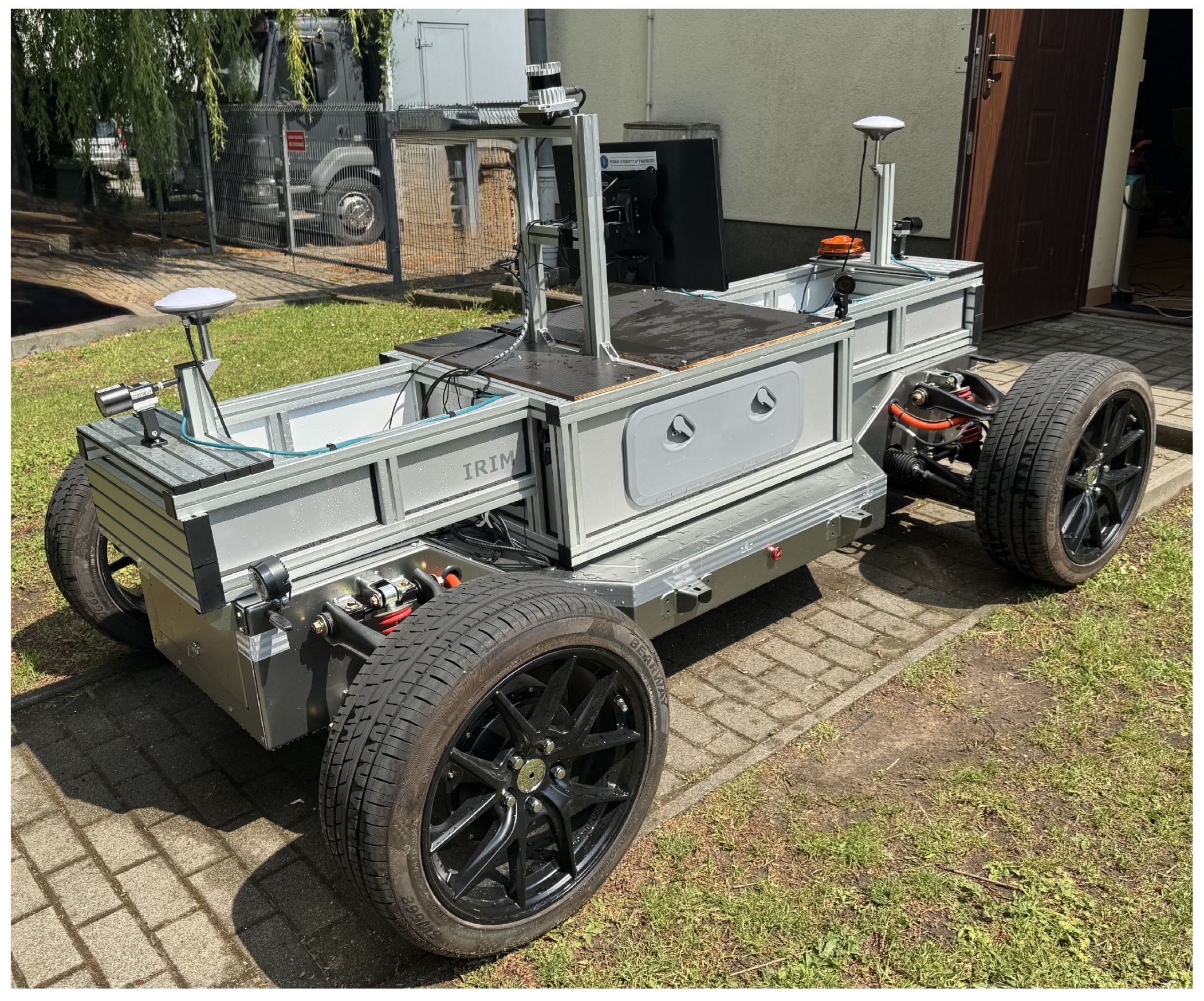
Efficient deployment of semantic segmentation models in real-world robotic systems requires consideration of inference latency and computational resource usage. This section presents a detailed evaluation of latency, memory footprint, and GPU utilization across a range of encoder–decoder architectures tested at two different input resolutions.
Table 8 reports the inference performance of four state-of-the-art semantic segmentation architectures (U-Net, DeepLabv3+, FPN, SegFormer) each combined with three ImageNet-pre-trained encoders (MobileNetV4, ResNet-34, EfficientNet-B2). All models were benchmarked over 1000 forward passes using input images at resolutions of 960 × 608, with selected architectures being additionally evaluated at the reduced resolution of 480 × 304. It summarizes the following metrics: latency statistics (the minimum, maximum, mean inference time, standard deviation) all expressed in milliseconds; the GPU memory requirement for parameter loading in megabytes (MB); and the peak GPU utilization percentage during inference. Inference was measured by running each FP32 ONNX model on GPU via ONNX Runtime CUDA execution provider. In order to ensure experimental consistency, all evaluations were performed on a single computer equipped with an NVIDIA RTX 4070 GPU.
Among the evaluated configurations that were processing full-resolution images, DeepLabv3+ with MobileNetV4 delivered the shortest inference time, with an impressively low average inference time of , combined with tiny GPU memory footprint of just . This combination is ideal for any application where short inference time and minimal resource usage are critical.
In our experiments, MobileNetV4 outperformed other encoders in terms of processing speed across all evaluated models. Its mean of inference latency was below 9 ms for all model combinations. Additionally, MobileNetV4 demonstrated minimal peak GPU utilization in all model–encoder configurations except when integrated with FPN. EfficientNet-B2, despite requiring intermediate memory for parameter loading, achieved the longest mean inference time for the three model variants.
When ranking architectures by overall efficiency, DeepLabv3+ with MobileNetV4 ranks first, closely followed by FPN+ MobileNetV4. When paired with MobileNetV4, FPN achieves an average inference time of , while requiring only of GPU memory. This configuration is preferable when the improved boundary detail offered by multi-scale feature fusion outweighs the slight increase in latency. For systems where the GPU must be shared with other processes, SegFormer paired with MobileNetV4 presents a strong alternative. Despite a higher average latency of 8.59 ms, it requires only 24 MB of memory and reaches peak utilization of approximately 47%.
Reducing input image resolution by a factor of four led to efficiency gains, with average latency times decreasing by over 2.5 times and maximum GPU usage dropping by 16 percentage points during tests of both architectures. The U-Net with ResNet-34 configuration achieved both the shortest single inference time of , and minimum mean latency of .
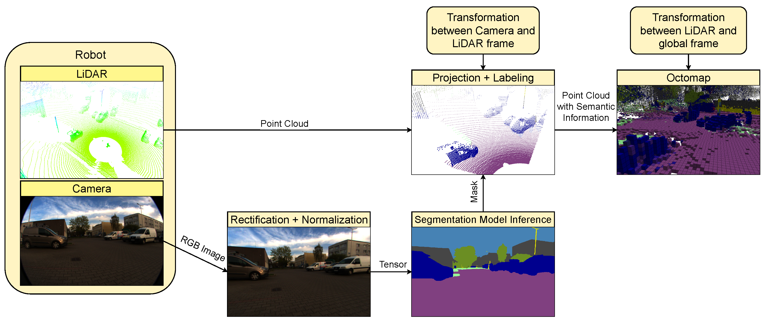
4.3. Semantic OctoMaps Validation
To compare the quality of segmentation in the 3D space, we processed recorded sequences from rosbag files through the ROS2 node while employing the complete set of previously trained models. We set the OctoMap resolution to 25 cm, enabling the creation of a large yet relatively precise representation of the environment. For analysis, we obtained a point cloud formed by points located at the centers of occupied voxels in the map. Approximately 16% of points were removed in both scenarios as they were not assigned a color during the mapping process (these points maintained the default pure white color because the voxel does not have the required number of measurements—in our implementation, a point must be located inside the voxel in two separate scans). To assign a point to a particular class, its color values must not differ by more than 5 units in any channel from the reference color values listed in
Table 1. We define non-classified points (NC) as those which, despite having assigned color values, could not be assigned to any semantic class by not meeting the color difference criterion. This stems from color blending in the OctoMap when a particular spatial region was repeatedly annotated with different labels. In such a case, there is insufficient confidence for the point to be assigned to any semantic class. To establish ground truth data, scene elements were manually annotated with cuboids.
We split the experiment into several phases. First, we evaluated segmentation performance using all model–encoder combinations using the default image resolution. Subsequently, we extended the analysis with a comparison using downscaled images and maps created by models trained on masks produced by Grounding DINO and SAM2. The results are presented in
Table 9,
Table 10, and
Table 11, respectively. These tables store the following metrics: accuracy (ACC), weighted F1-score (wF1), where the weights are directly proportional to the fraction of points of each class in the complete map, and the percentage of unclassified voxels (NC). The index
f appended to the metric name indicates that the value was computed for the subset of points after filtering out those not assigned to any class. Finally, we compared F1-scores achieved for individual classes by top-performing models for each encoder type across all three experimental setups. The metrics are visualized in the graphs shown in
Figure 6,
Figure 7 and
Figure 8. In
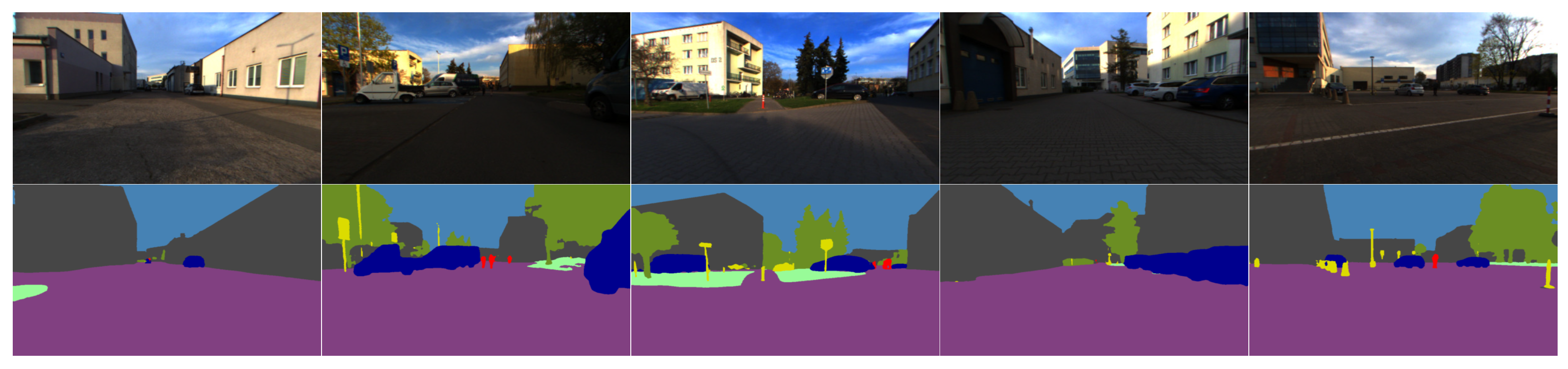
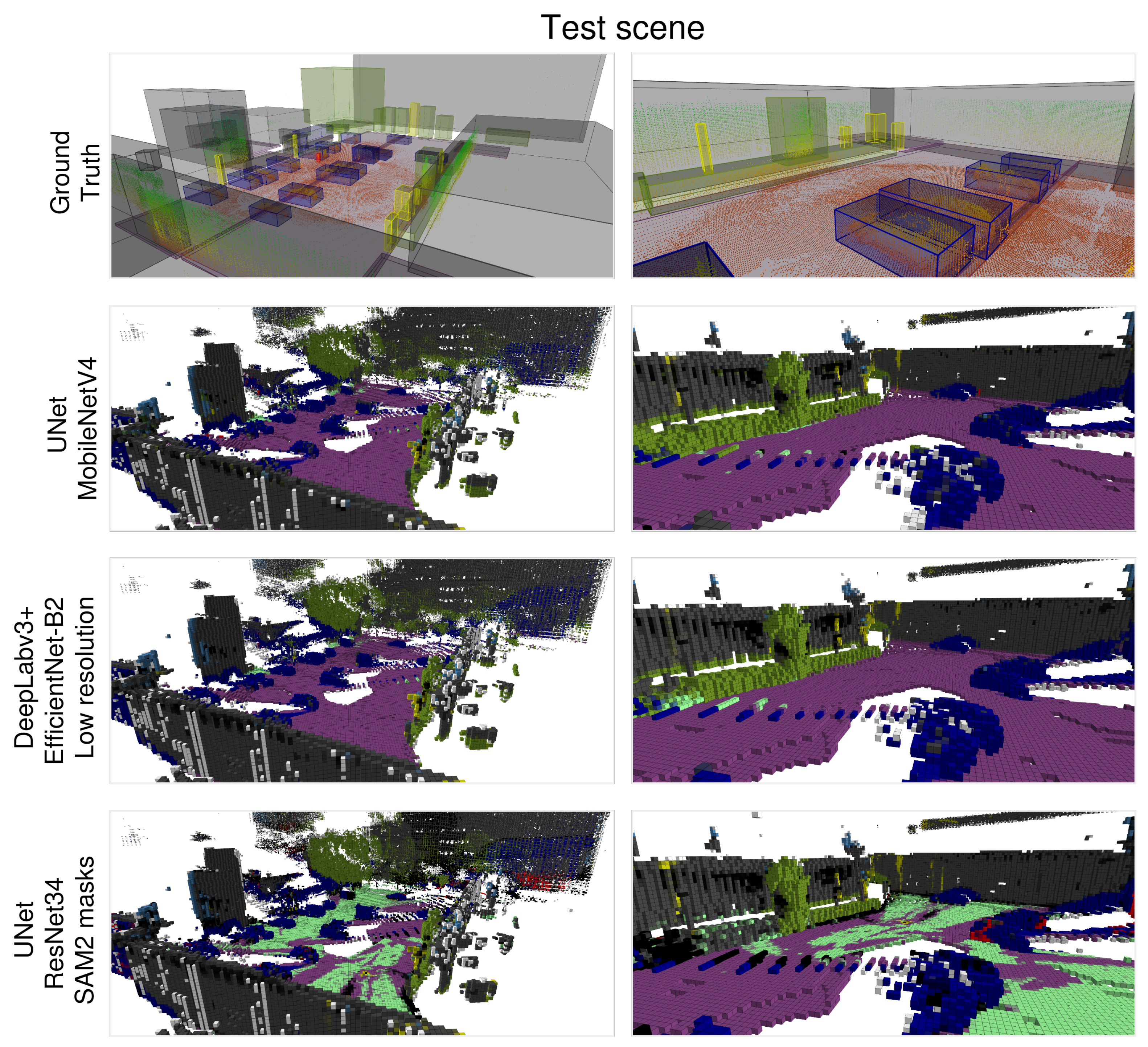
Figure 9 and
Figure 10, we present manual ground truth labels alongside OctoMaps generated using selected segmentation approaches.
As shown in
Table 9, FPN coupled with the lightweight MobileNetV4 backbone achieves the highest accuracy on validation scene
, filtered accuracy
, filtered weighted
-score
, and low unclassified rate
on the validation scene. It also generalizes well to the test scene, with
and
, indicating that hierarchical feature integration with a lightweight encoder can outperform other configurations in both accuracy and efficiency. On the other hand, DeepLabv3+ paired with EfficientNet-B2 not only achieves the lowest unclassified-voxel rate on the test split (
) but also maintains competitive overall performance (
,
). This configuration demonstrates also an optimal balance between reducing unclassified areas and maintaining high segmentation accuracy. Furthermore, U-Net with a MobileNetV4 backbone delivers strong performance, particularly on the test scene, where it achieves the highest accuracy among all combinations (
) and the highest filtered weighted
-score (
). On the validation scene, it records
,
,
, and an unclassified-voxel rate of
. In the test scenario, the relatively low
indicates that U-Net+MobileNetV4 produces one of the most complete semantic maps.
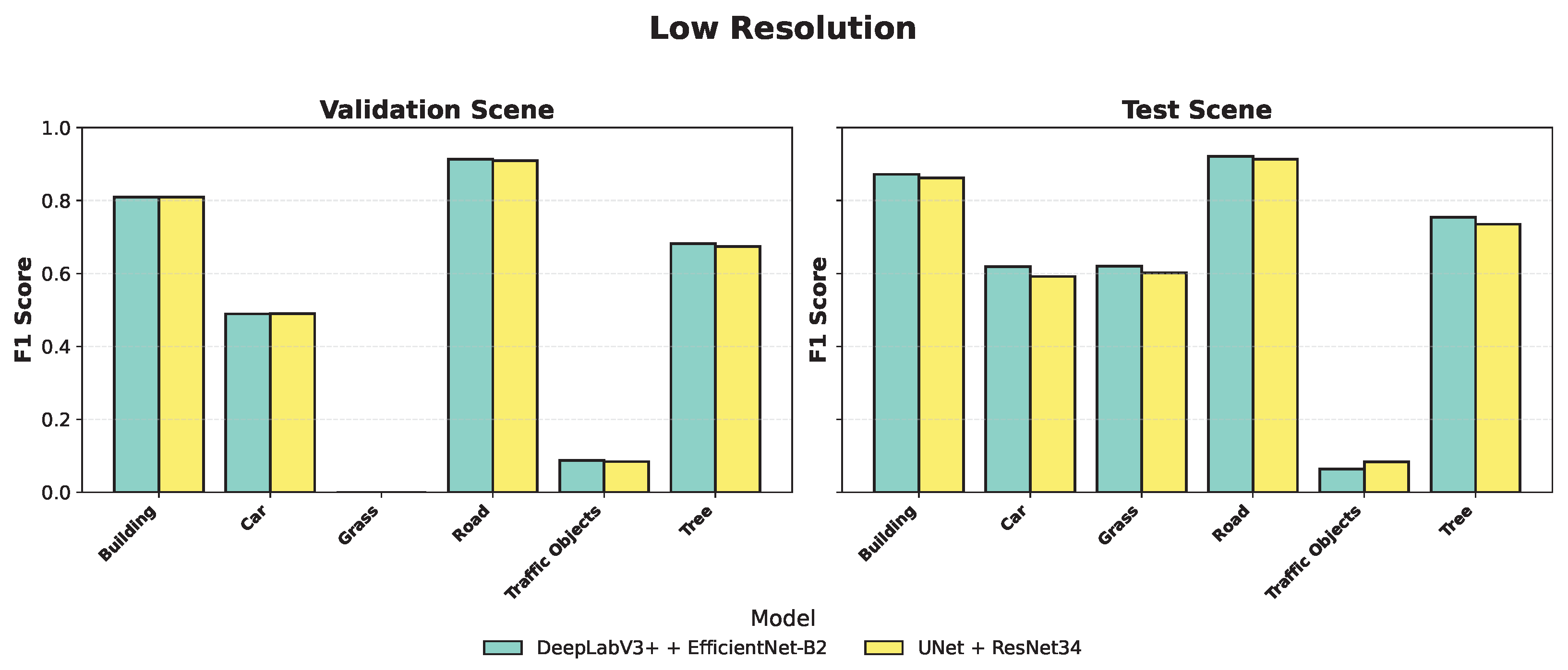
As reported in
Table 10, at lower resolution, U-Net with ResNet-34 attained the lowest unclassified-voxel rate (
) on the test split, producing the most complete occupancy map-crucial for robotic scenarios that depend on continuous environment reconstruction. Moreover, on the test scene, U-Net + ResNet-34 achieves the lowest unclassified-voxel rate (
), providing the most complete semantic coverage even at reduced resolution, with only marginal losses in overall accuracy and weighted
. In practice, downscaling can significantly reduce computational cost while sacrificing only a few percentage points of filtered accuracy and
In
Table 11, we show that masks generated by GroundingDINO and SAM2 in their current implementation demonstrate inadequate semantic precision, leading to an increase in
of approximately 20–30% and a reduction in
of roughly 10–15%. For instance, on the validation scene, DeepLabv3+ + EfficientNet-B2 achieves
,
, and
, while U-Net + ResNet-34 records
,
, and
. These results demonstrate that GroundingDINO+SAM2 masks lack the precision necessary for reliable semantic mapping.
In
Figure 6,
Figure 7 and
Figure 8, we compare the per-class F1-scores of the top-performing models across validation and test scenes. The model based on DeepLabv3+ with EfficientNet-B2 achieves high F1-scores of 0.91 for the Road class, 0.87 for Building, and 0.76 for Tree, demonstrating consistently strong performance across both validation and test scenes. The U-Net with MobileNetV4, despite its lightweight architecture, delivers stable performance across both validation and test scenes. On the test scene, it attains F1-scores of 0.91 for Road, 0.87 for Building, and 0.76 for Tree, matching the performance of DeepLabv3+ with EfficientNet-B2. On the validation scene, it maintains strong results with scores of 0.92, 0.88, and 0.76 for the same classes. The U-Net model with a ResNet-34 encoder shows slightly lower performance across most categories, reaching F1-scores of 0.86 for Road, 0.79 for Building, and 0.75 for Tree. In contrast, the classes Traffic objects and Grass remain the most challenging for all evaluated models, with F1-scores consistently falling below 0.3, particularly when models are trained on SAM2-derived annotations. This observation indicates that segmentation models tend to underperform when detecting objects that are small in spatial extent or infrequent within the training distribution.


