

Comparison of Acceleration Amplification for Seismic Behavior Characteristics Analysis of Electrical Cabinet Model: Experimental and Numerical Study

Abstract
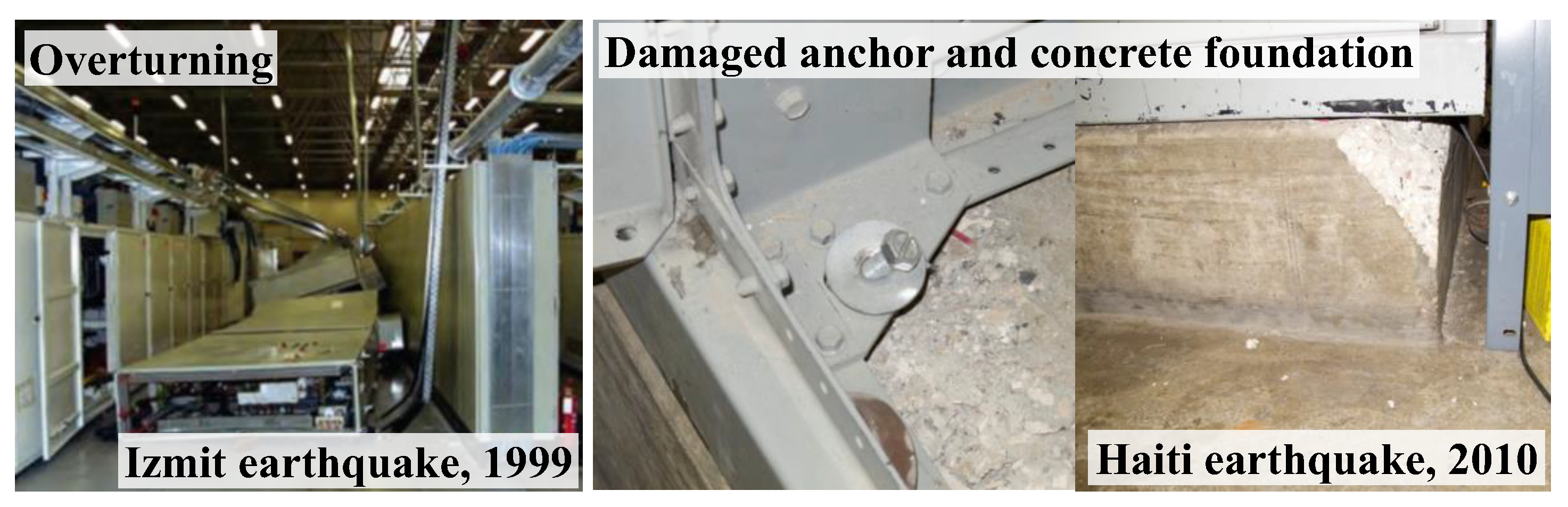
1. Introduction
2. Experimental Test Overview
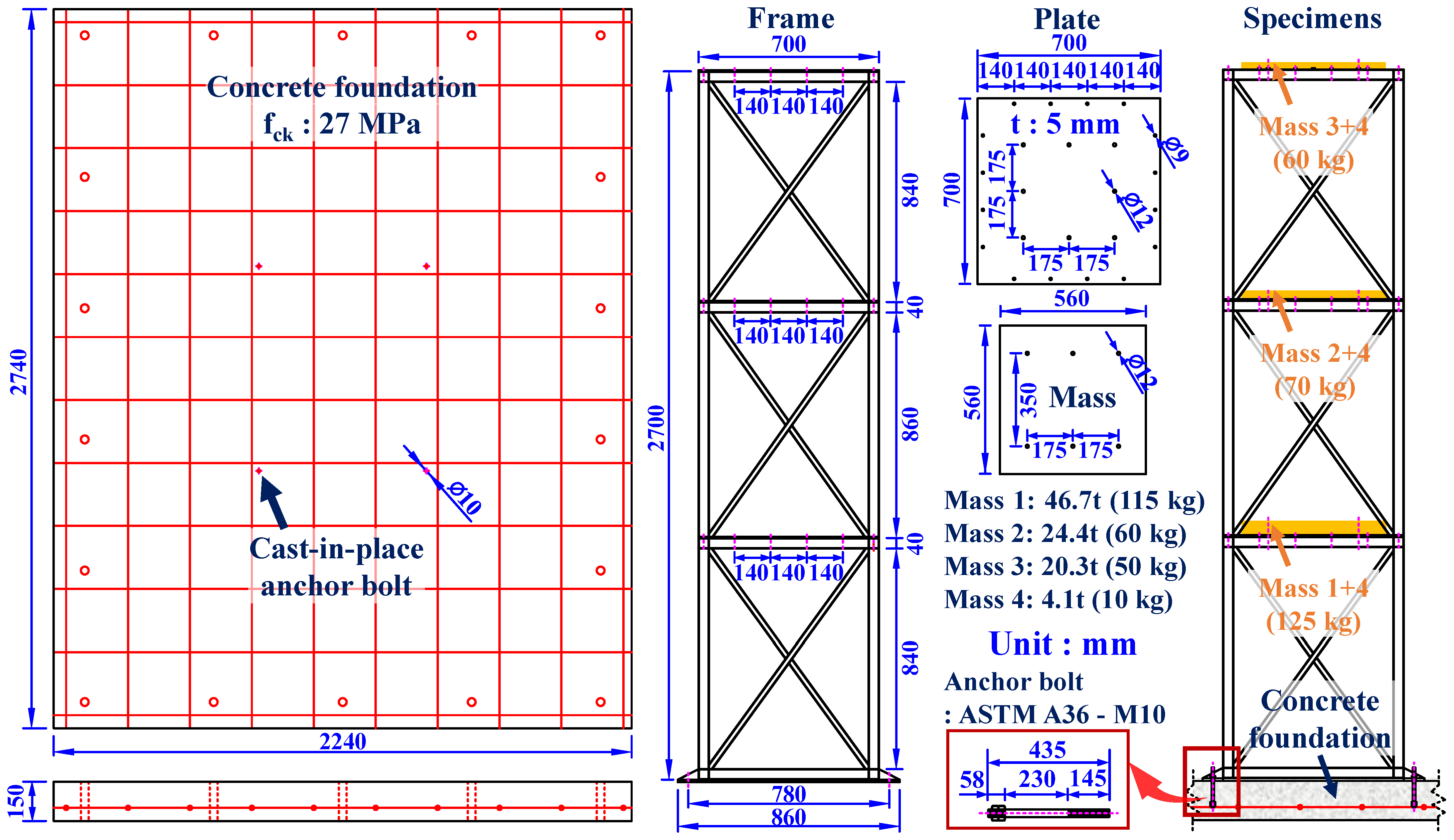
2.1. Design and Fabrication of Specimen
2.2. Experimental Setup
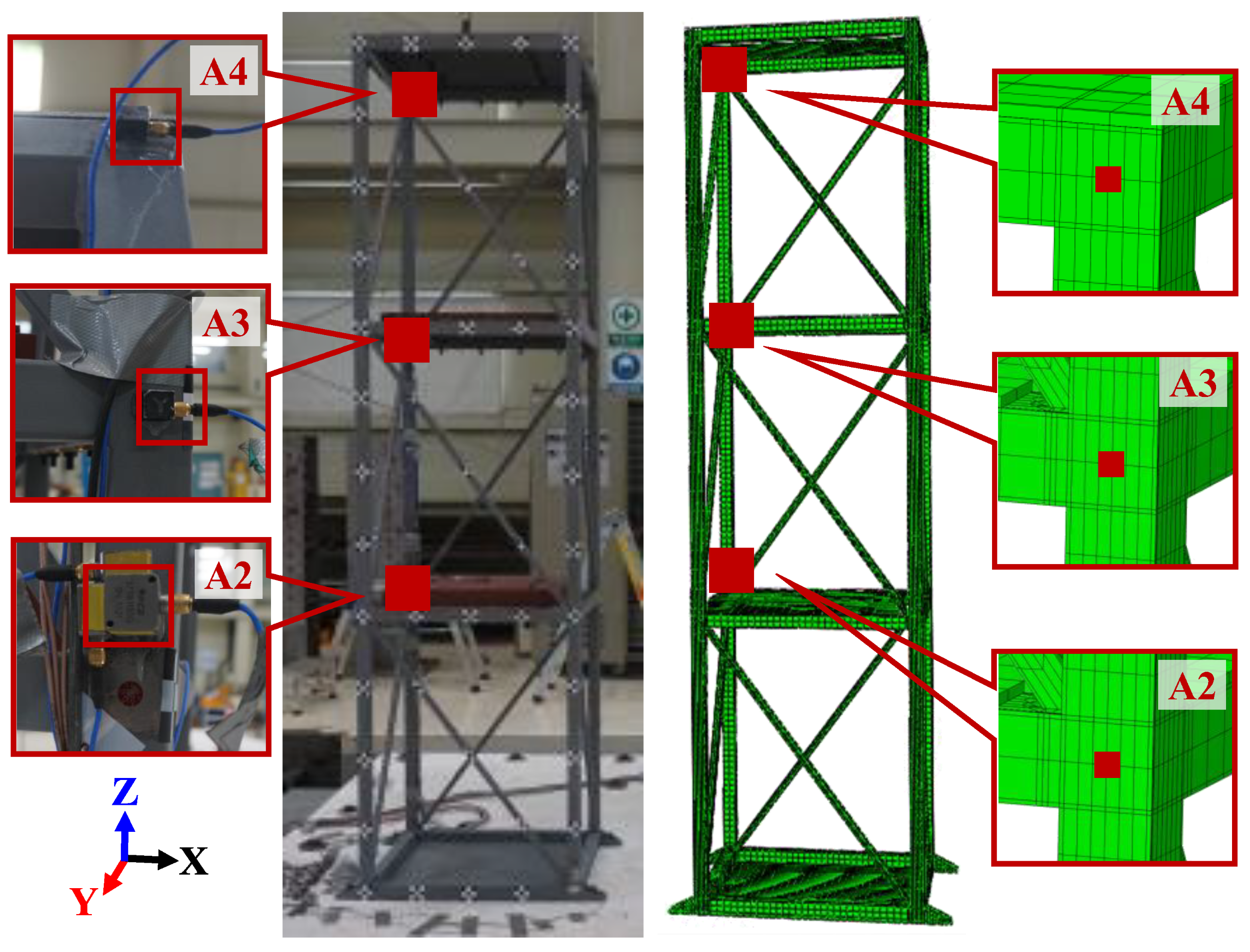
2.2.1. Specimen Installation and Setup
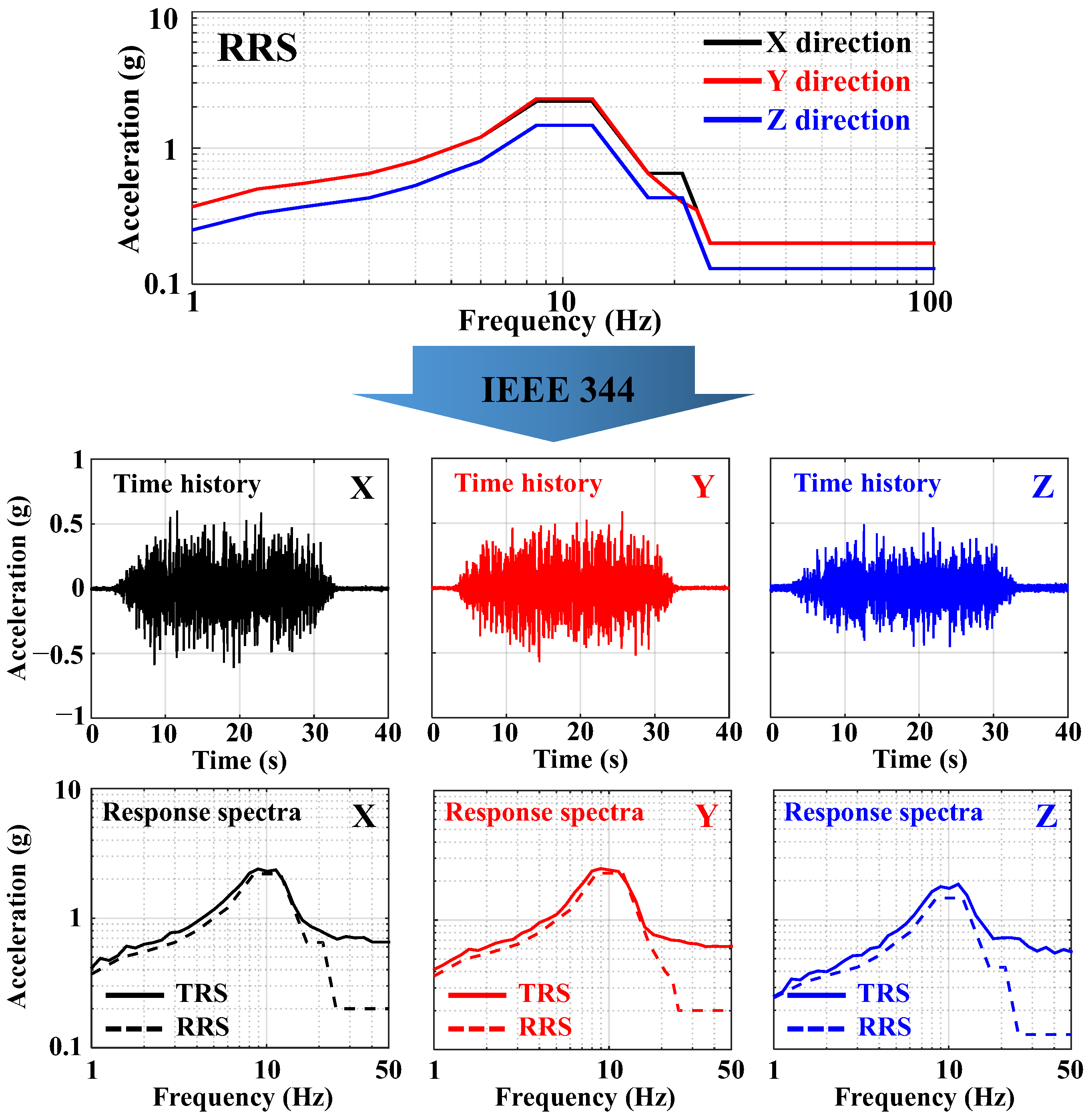
2.2.2. Input Seismic Motion
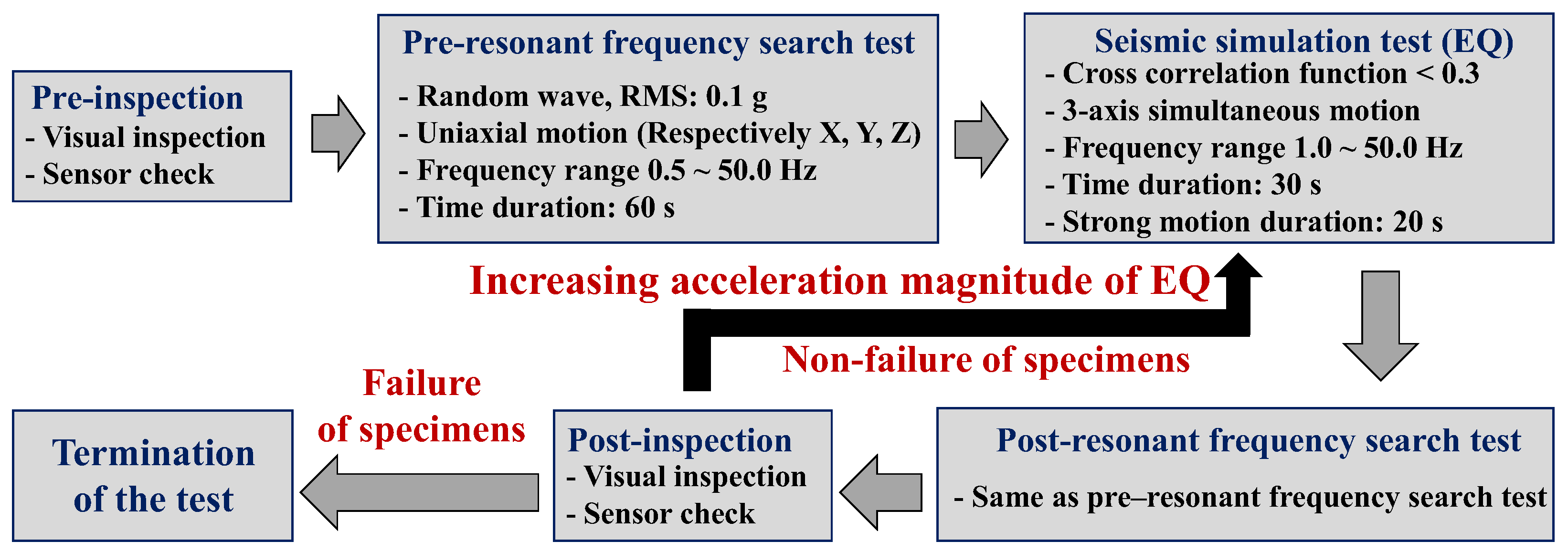
2.2.3. Experimental Procedure and Method
2.3. Experimental Results
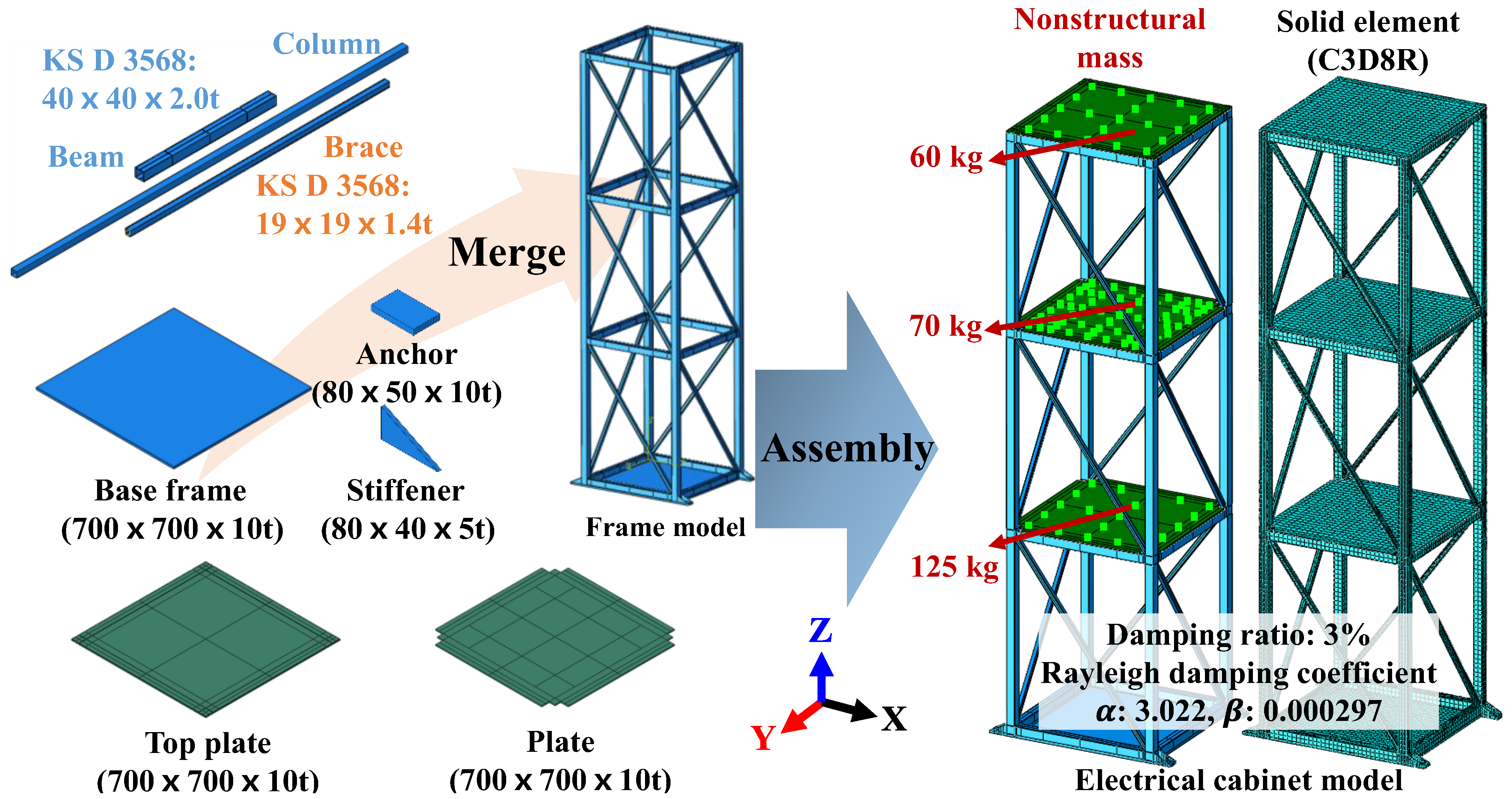
3. Numerical Analysis Overview
3.1. Verification of Numerical Model
3.2. Seismic Response Analysis
4. Analysis and Comparison of Results
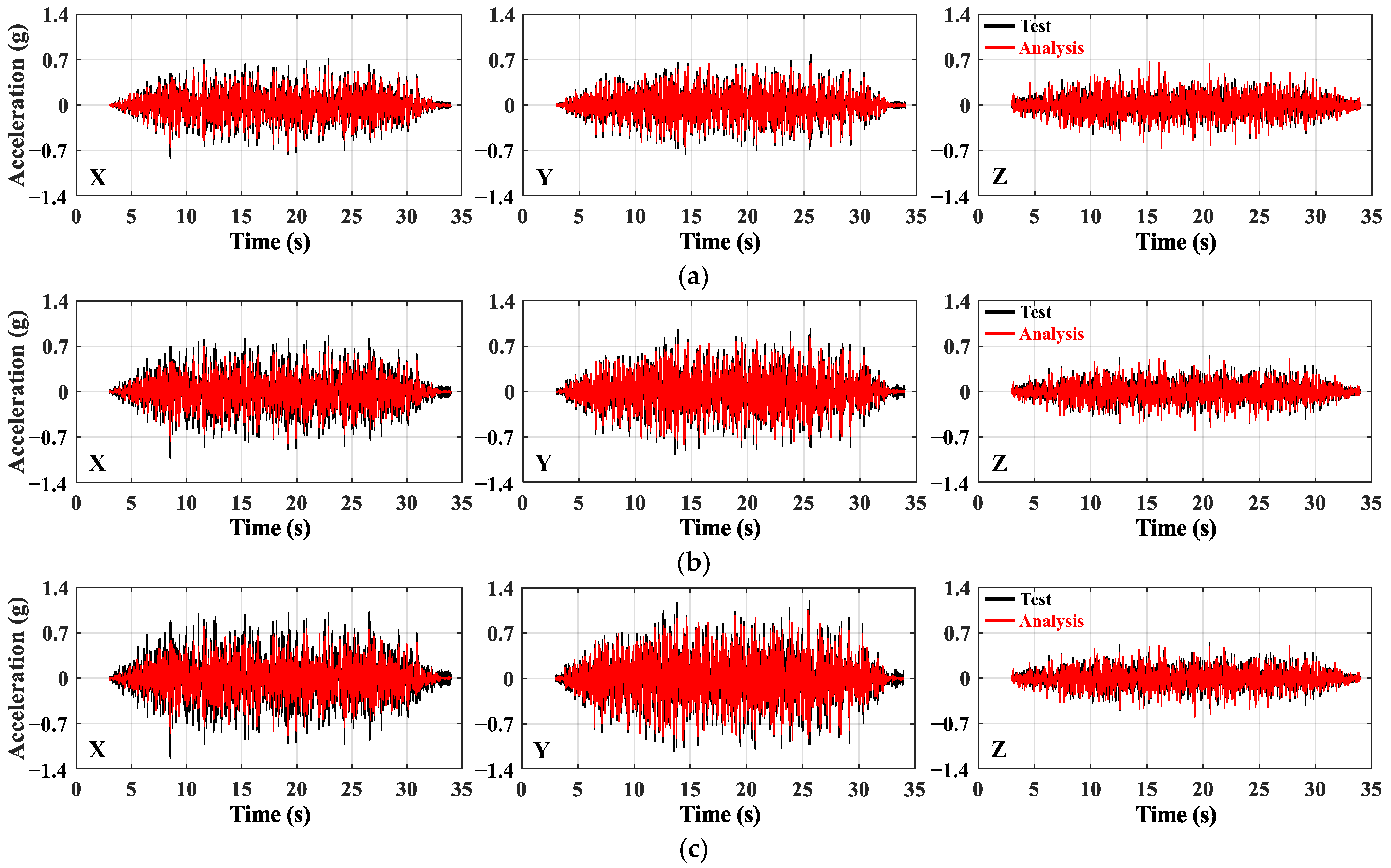
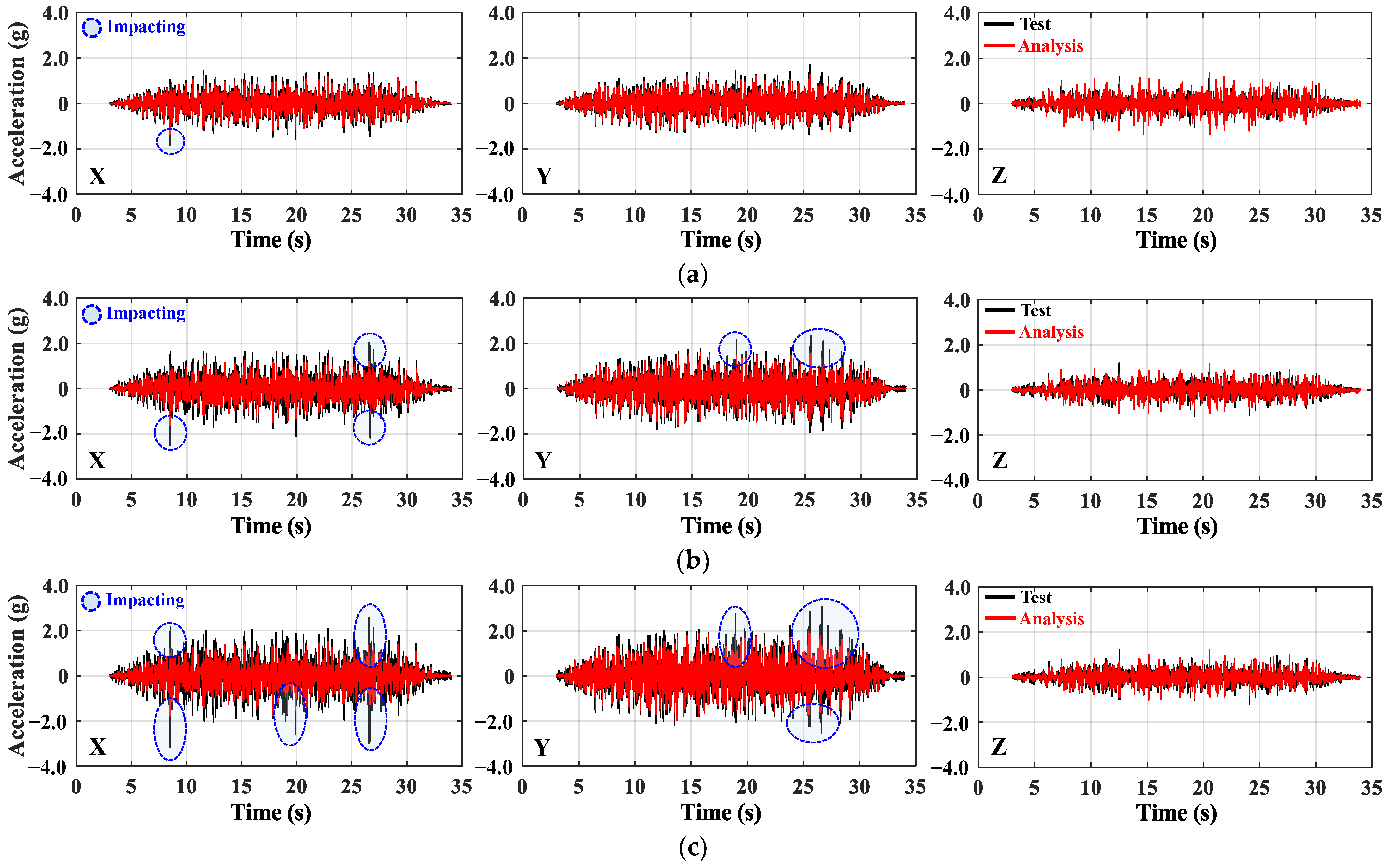
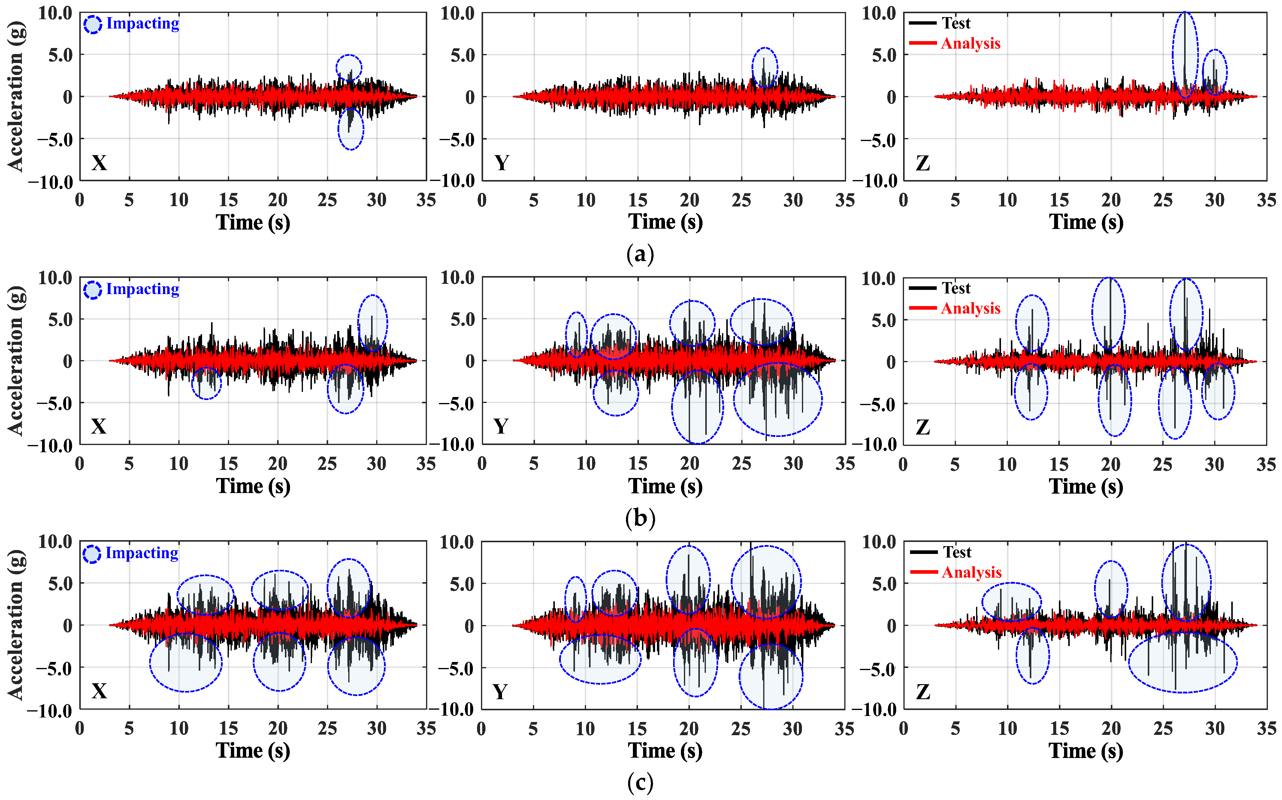
4.1. Comparison of Acceleration Response Time Histories
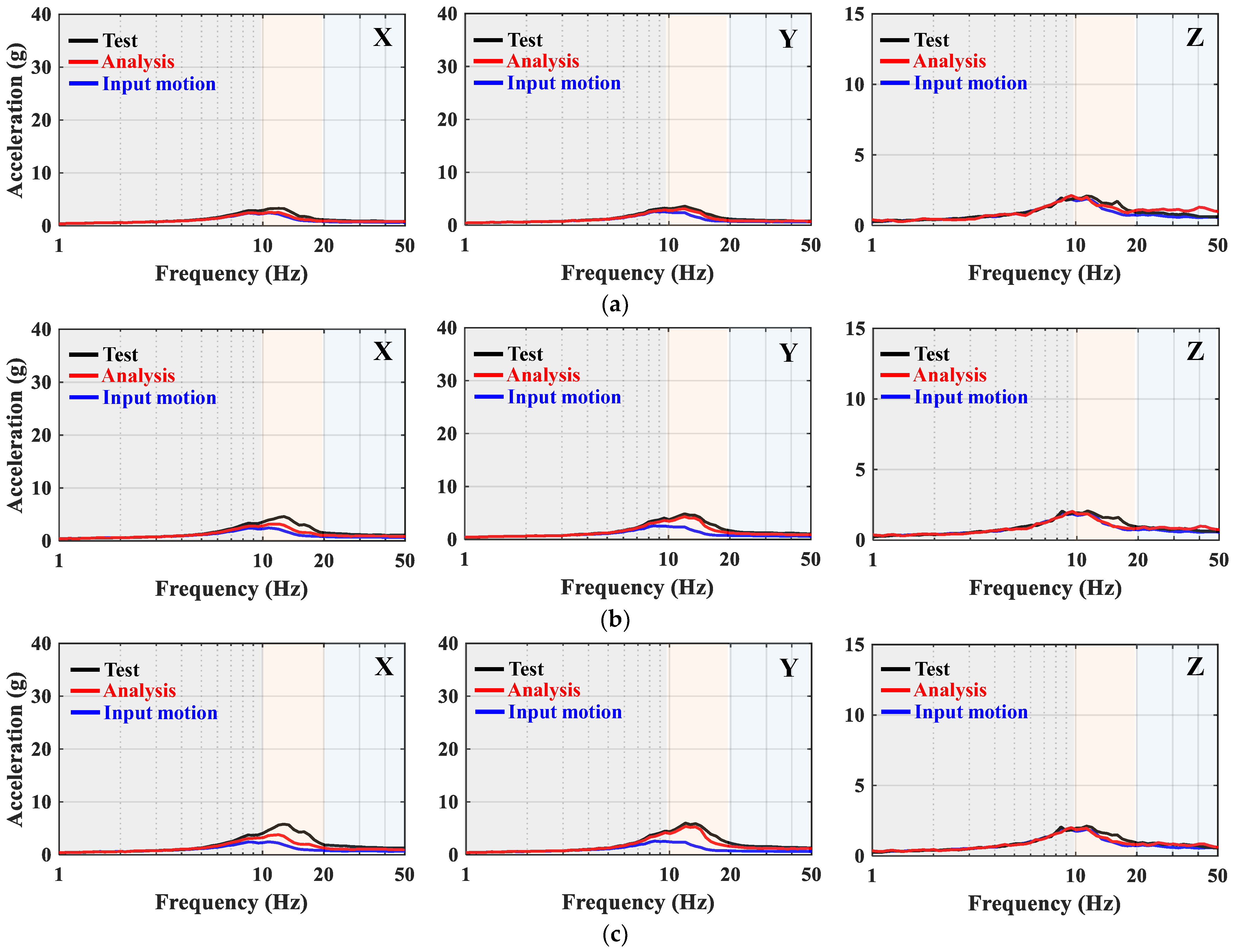
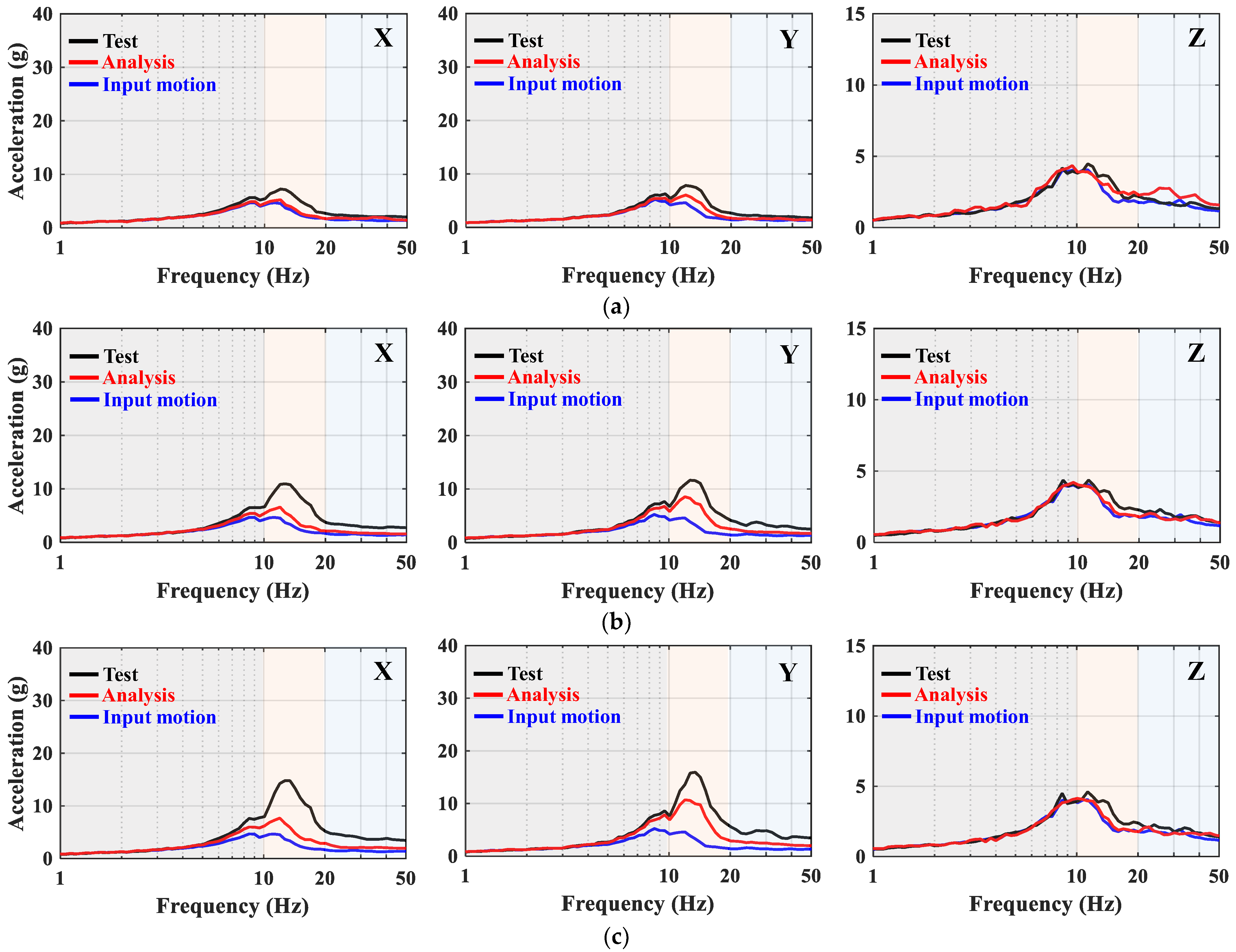
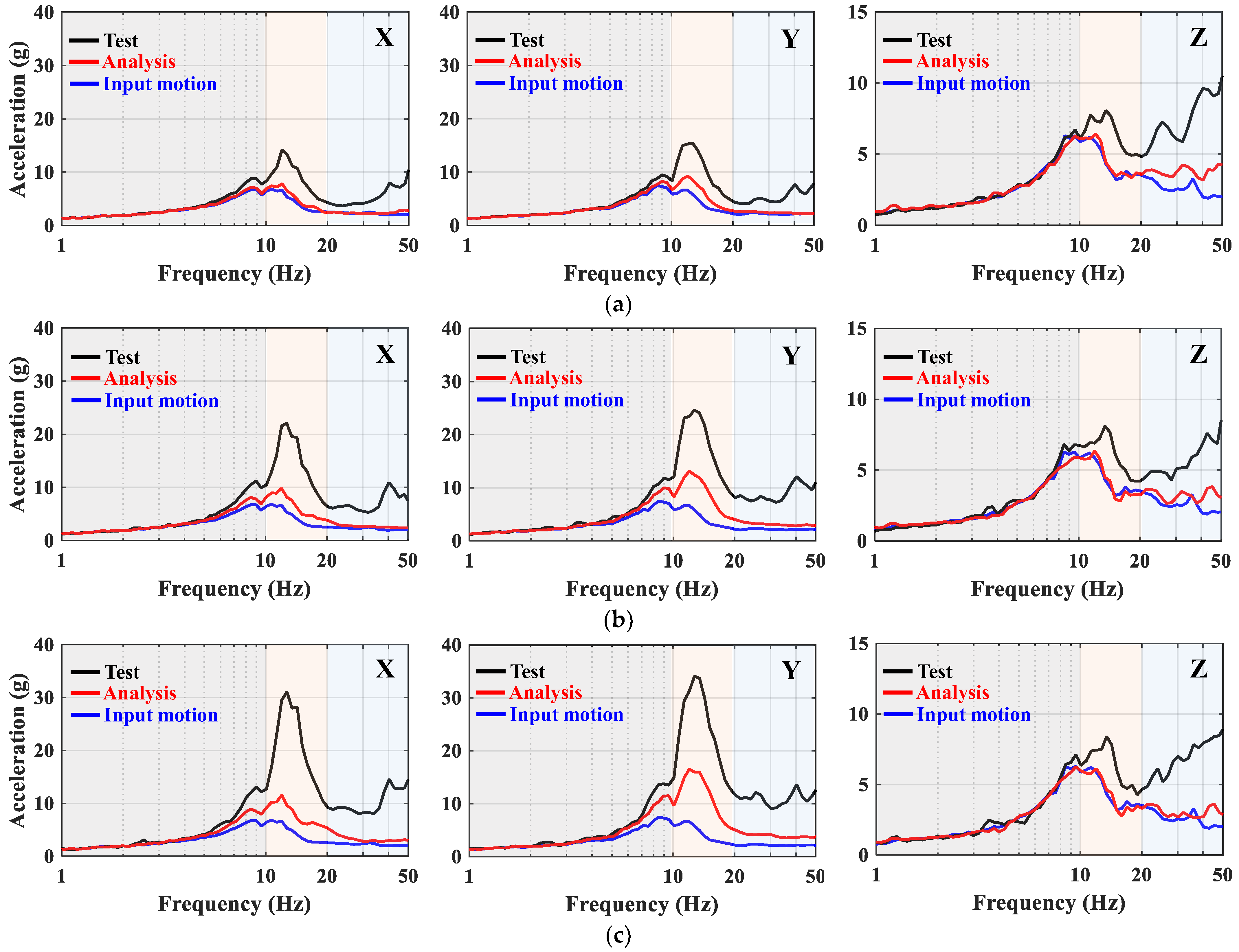
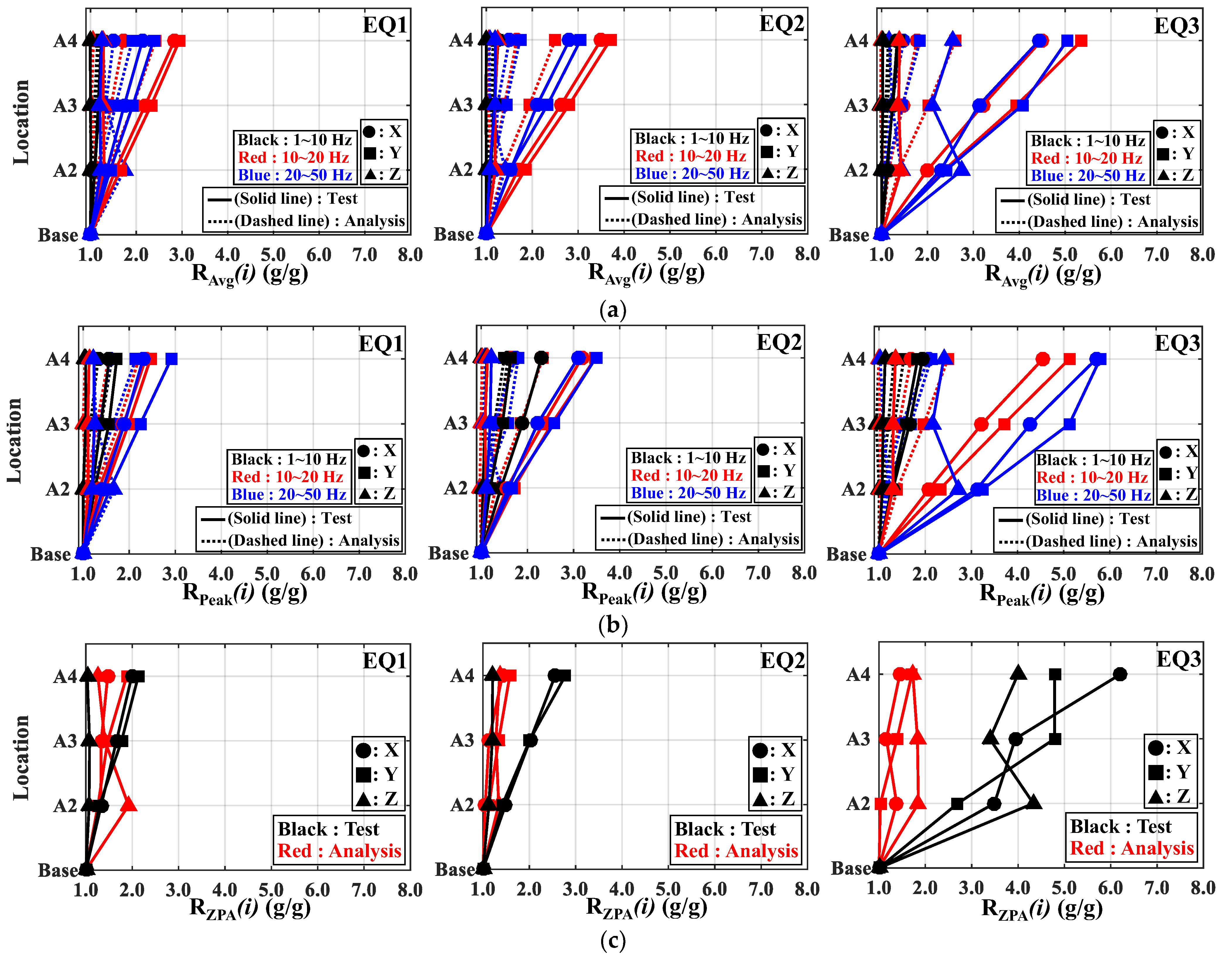
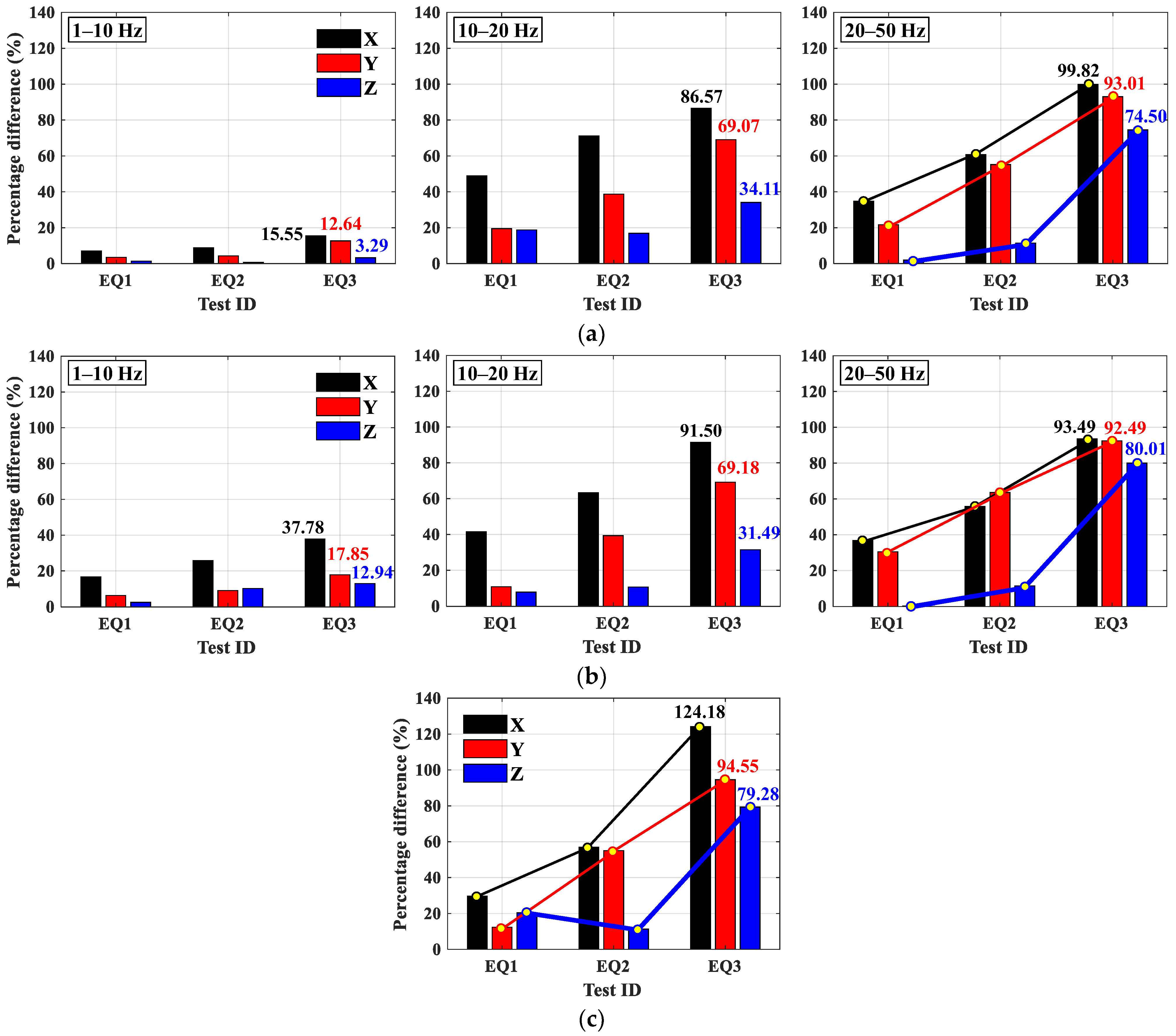
4.2. Comparison of Acceleration Response Spectra
5. Conclusions
Author Contributions
Funding
Institutional Review Board Statement
Informed Consent Statement
Data Availability Statement
Conflicts of Interest
Abbreviations
| NPP | Nuclear power plant |
| ICRS | In-cabinet response spectrum |
| MCC | Motor control center |
| RRS | Required response spectrum |
| TRS | Test response spectrum |
| FRS | Floor response spectrum |
| ZPA | Zero period acceleration |
| PD | Percentage difference |
| RMS | Root mean square |
| RMQ | Root mean quad |
References
- Goodno, B.J.; Gould, N.C.; Caldwell, P.; Gould, P.L. Effects of the January 2010 Haitian earthquake on selected electrical equipment. Earthq. Spectra 2011, 27, S251–S276. [Google Scholar] [CrossRef]
- Shang, Q.; Zuo, H.; Wen, L.; Li, Z.; Sun, G.; Pan, P.; Wang, T. Seismic resilience of internet data center building with different disaster mitigation techniques. Resilient Cities Struct. 2022, 1, 42–56. [Google Scholar] [CrossRef]
- Ikbal, M.K.H.; Nguyen, D.V.; Kim, S.; Kim, D. Seismic evaluation of different types of electrical cabinets in nuclear power plants considering coupling effects: Experimental and numerical study. Nucl. Eng. Technol. 2023, 55, 3472–3484. [Google Scholar] [CrossRef]
- United States Nuclear Regulatory Commission (USNRC). Identification of New Unresolved Safety Issues Relating to Nuclear Power Plant Stations (NUREG-0705); USNRC: Washington, DC, USA, 1981.
- United States Nuclear Regulatory Commission (USNRC). Seismic Qualification of Equipment in Operating Nuclear Power Plants (NUREG-1030); USNRC: Washington, DC, USA, 1987.
- International Atomic Energy Agency (IAEA). Seismic Design and Qualification for Nuclear Power Plants; IAEA: Vienna, Austria, 2004. [Google Scholar]
- Lin, F.R.; Chai, J.F.; Lai, Z.Y.; Chou, P.F.; Wu, Y.C. Experimental study for seismic demands on in-cabinet equipment in NPPs. J. Chin. Inst. Eng. 2014, 37, 833–844. [Google Scholar] [CrossRef]
- Chang, S.J.; Jeong, Y.S.; Eem, S.H.; Choi, I.K.; Park, D.U. Evaluation of MCC seismic response according to the frequency contents through the shake table test. Nucl. Eng. Technol. 2021, 53, 1345–1356. [Google Scholar] [CrossRef]
- Jeong, Y.S.; Eem, S.H.; Jeon, B.G.; Park, D.U. Evaluation of structural and functional behavior of battery charger for low/high-frequency motions in NPP. Appl. Sci. 2022, 12, 4328. [Google Scholar] [CrossRef]
- Jeon, B.G.; Kim, S.W.; Chang, S.J.; Park, D.U.; Lee, H.P. Seismic behavior of simplified electrical cabinet model considering cast-in-place anchor in uncracked and cracked concretes. Nucl. Eng. Technol. 2023, 55, 4252–4265. [Google Scholar] [CrossRef]
- Nagai, M.; Minakawa, Y.; Hibino, K.; Takamatsu, N.; Ishida, N.; Yoshimura, E.; Maruyama, N.; Furuya, O. Shaking Table Test of Electrical Cabinet Considering Shock Vibration. In Proceedings of the 27th International Conference on Structural Mechanics in Reactor Technology, Yokohama, Japan, 3–8 March 2024. [Google Scholar]
- Zuo, H.; Sun, G.; Zhang, P.; Wang, M.; Li, J.; Shang, Q.; Wang, T. Shaking table tests of a switching power cabinet considering physical damage and functionality loss. Soil Dyn. Earthq. Eng. 2024, 177, 108421. [Google Scholar] [CrossRef]
- Shang, Q.; Zuo, H.; Zhang, X.; Li, Z.; Sun, G.; Zhang, P.; Li, J.; Wang, T. Shaking table tests of power distribution cabinets: Physical damage, post-earthquake functionality and seismic response evaluation. Structures 2024, 62, 106208. [Google Scholar] [CrossRef]
- Salman, K.; Tran, T.T.; Kim, D. Seismic capacity evaluation of NPP electrical cabinet facility considering grouping effects. J. Nucl. Sci. Technol. 2020, 57, 800–812. [Google Scholar] [CrossRef]
- Tran, T.T.; Cao, A.T.; Kim, D.; Chang, S.K. Seismic vulnerability of cabinet facility with tuned mass dampers subjected to high-and low-frequency earthquakes. Appl. Sci. 2020, 10, 4850. [Google Scholar] [CrossRef]
- Lee, S.M.; Jeon, B.G.; Kim, S.W.; Yun, D.W.; Jung, W.Y. Evaluating the applicability of seismic retrofit of an electric cabinet in a power plant. Struct. Build. 2024, 177, 589–605. [Google Scholar] [CrossRef]
- Gupta, A.; Rustogi, S.K.; Gupta, A.K. Reconciliation of Experimental and Analysis Results for Switchgear Incabinet Spectra. In Proceedings of the 15th International Conference on Structural Mechanics in Reactor Technology, Seoul, Republic of Korea, 15–20 August 1999. [Google Scholar]
- Ries, M.; Hahn, T.; Henkel, F.O. Seismic Qualification of an Electrical Cabinet: Comparison of Analysis and Test Results. In Proceedings of the 24th International Conference on Structural Mechanics in Reactor Technology, Busan, Republic of Korea, 20–25 August 2017. [Google Scholar]
- Son, H.; Park, S.; Jeon, B.G.; Jung, W.Y.; Choi, J.; Ju, B.S. Seismic qualification of electrical cabinet using high-fidelity simulation under high frequency earthquakes. Sustainability 2020, 12, 8048. [Google Scholar] [CrossRef]
- Son, H.; So, W.B.; Jeon, B.G.; Jung, W.Y.; Ju, B.S. Dynamic characteristics of double-door electrical cabinet by 3D finite element analysis model. J. Korean Soc. Adv. Compos. Struct. 2020, 11, 60–66. [Google Scholar] [CrossRef]
- Salman, K.; Cho, S.G. Effect of frequency content of earthquake on the seismic response of interconnected electrical equipment. CivilEng 2020, 1, 198–215. [Google Scholar] [CrossRef]
- Jeon, B.G.; Son, H.Y.; Eem, S.H.; Choi, I.K.; Ju, B.S. Dynamic characteristics of single door electrical cabinet under rocking: Source reconciliation of experimental and numerical findings. Nucl. Eng. Technol. 2021, 53, 2387–2395. [Google Scholar] [CrossRef]
- Ruggieri, S.; Vukobratović, N. The influence of torsion on acceleration demands in low-rise RC buildings. Bull. Earthq. Eng. 2024, 22, 2433–2468. [Google Scholar] [CrossRef]
- Llambias, J.M.; Sevant, C.J.; Shepherd, D.J. Non-Linear Response of Electrical Cubicles for Fragility Estimation. In Proceedings of the 10th International Conference on Structural Mechanics in Reactor Technology, Anaheim, CA, USA, 22–27 August 1989. [Google Scholar]
- Yang, J.; Rustogi, S.K.; Gupta, A. Rocking stiffness of mounting arrangements in electrical cabinets and control panels. Nucl. Eng. Des. 2003, 219, 127–141. [Google Scholar] [CrossRef]
- Yun, D.W.; Jeon, B.G.; Jung, W.Y.; Chang, S.J.; Shin, Y.J. Analysis of anchorage behavior characteristics of the electrical cabinet using shaking table tests. Korean Soc. Noise Vib. Eng. 2019, 29, 43–50. [Google Scholar] [CrossRef]
- Cho, S.G.; Salman, K. Seismic demand estimation of electrical cabinet in nuclear power plant considering equipment-anchor-interaction. Nucl. Eng. Technol. 2022, 54, 1382–1393. [Google Scholar] [CrossRef]
- Federal Emergency Management Agency (FEMA). Reducing the Risks of Nonstructural Earthquake Damage—A Practical Guide (FEMA E-74); FEMA: Washington, DC, USA, 2012.
- Merz, K.L.; Ibanez, P. Guidelines for estimation of cabinet dynamic amplification. Nucl. Eng. Des. 1990, 123, 247–255. [Google Scholar] [CrossRef]
- Electric Power Research Institute (EPRI). The Effects of High-Frequency Ground Motion on Structures, Components, and Equipment in Nuclear Power Plants; EPRI: Palo Alto, CA, USA, 2007. [Google Scholar]
- Bandyopadhyay, K.K.; Hofmayer, C.H.; Kassir, M.K.; Pepper, S.E. Dynamic Amplification of Electrical Cabinets (NUREG/CR-5203); Brookhaven National Laboratory (BNL): New York, NY, USA, 1988.
- Lee, B.J.; Berak, E.G.; Passalugo, P.N. Effect of base shim plates on seismic qualification of electrical control panels. Am. Soc. Mech. Eng. 1990, 197, 301–306. [Google Scholar]
- Lee, B.J.; Abou-Jaoude, C.; De Estrada, M. Issues of control panel rigidity in seismic qualification. Seism. Eng. 1991, 220, 283–287. [Google Scholar]
- Lee, B.J.; Abou-Jaoude, C. Effect of base uplift on dynamic response of electrical and mechanical equipment. Seism. Eng. 1992, 237, 45–150. [Google Scholar]
- Latif, A.; Salman, K.; Kim, D. Seismic response of electrical cabinets considering primary-secondary structure interaction with contact nonlinearity of anchors. J. Nucl. Sci. Technol. 2022, 59, 757–767. [Google Scholar] [CrossRef]
- Song, J.; Pan, Y.; Wang, T.; Chen, Q. Seismic response and fragility analysis of railway station typical signal cabinets. Structures 2024, 68, 107185. [Google Scholar] [CrossRef]
- Lin, W.T.; Wu, Y.C.; Huang, C.C. Frequency analysis of the motor control centers in a nuclear power plant using testing and simulating methods. Appl. Mech. Mater. 2014, 479–480, 1045–1050. [Google Scholar] [CrossRef]
- American Concrete Institute (ACI). Qualification of Post-Installed Mechanical Anchors in Concrete and Commentary (ACI 355.2-07); ACI: Farmington Hills, MI, USA, 2007. [Google Scholar]
- ASTM A36/A36M-19; Standard Specification for Carbon Structural Steel. American Society for Testing and Materials (ASTM) International: Conshohocken, PA, USA, 2019.
- Gupta, A.; Rustogi, S.K.; Gupta, A.K. Ritz vector approach for evaluating incabinet response spectra. Nucl. Eng. Des. 1999, 190, 255–272. [Google Scholar] [CrossRef]
- Salman, K.; Tran, T.T.; Kim, D. Grouping effect on the seismic response of cabinet facility considering primary-secondary structure interaction. Nucl. Eng. Technol. 2020, 52, 1318–1326. [Google Scholar] [CrossRef]
- Singh, S.; Gupta, A. Understanding the seismic response of electrical equipment subjected to high–frequency ground motions. Prog. Nucl. Energy 2021, 140, 103915. [Google Scholar] [CrossRef]
- Chang, S.J.; Lee, Y.L.; Jeong, Y.S.; Kim, J.B.; Park, D.U. Seismic Test Report for 1st Limit State Test of Load Center; Seismic Research and Test Center (SESTEC), Institute for Research and Business Development Foundation, Pusan National University: Yangsan, Republic of Korea, 2024. [Google Scholar]
- Jeon, B.G.; Park, D.U.; Kim, S.W.; Chang, S.J.; Eem, S.; Park, J. A case study on the failure of the electrical panel of nuclear power plants by shaking table tests. Nucl. Eng. Technol. 2025, 57, 103533. [Google Scholar] [CrossRef]
- KS D 3568; Carbon Steel Square Pipes for General Structural Purposes. Korea Agency for Technology and Standards (KS): Eumseong, Republic of Korea, 2023.
- Rivera-Rosarino, H.T.; Powell, J.S. Installation Torque Tables for Noncritical Applications (NASA/TM-2017-219475); National Aeronautics and Space Administration (NASA): Washington, DC, USA, 2017.
- IEEE Std 344; IEEE Standard for Seismic Qualification of Equipment for Nuclear Power Generating Stations. The Institute of Electrical and Electronics Engineers (IEEE): Piscataway, NJ, USA, 2013.
- Kim, J.B.; Kim, S.K.; Seo, K.S.; Lee, J.C. Stress-Strain Curves of Mild Carbon Steels for Decommissioning Wastes Transportation Container. In Proceedings of the Korean Nuclear Society Autumn Meeting, Seoul, Republic of Korea, 23–25 October 2019. [Google Scholar]
- Kang, H.S.; Kim, T.S. An experimental study on buckling behaviors of cold-formed carbon steel square hollow section compressive members under a concentric axial load. J. Archit. Inst. Korea 2022, 38, 273–282. [Google Scholar]
- United States Nuclear Regulatory Commission (USNRC). Recommendations for Revision of Seismic Damping Values in Regulatory Guide 1.61 (NUREG/CR-6919); USNRC: Washington, DC, USA, 2006.
- Jeon, B.G.; Chang, S.J.; Kim, S.W.; Park, D.U.; Chun, N. Experimental study on the acceleration amplification ratio of cable terminations for electric power facilities. Energies 2024, 17, 5641. [Google Scholar] [CrossRef]
- Olieman, M.; Marin-Perianu, R.; Marin-Perianu, M. Measurement of dynamic comfort in cycling using wireless acceleration sensors. Procedia Eng. 2012, 34, 568–573. [Google Scholar] [CrossRef]
- Shah, S. Mesh Discretization Error and Criteria for Accuracy of Finite Element Solutions. In Proceedings of the 4th ASEAN ANSYS Users Conference, Singapore, 5–6 November 2002. [Google Scholar]
- Nahar, T.T.; Cao, A.T.; Kim, D. Effective safety assessment of aged concrete gravity dam based on the reliability index in a seismically induced site. Appl. Sci. 2021, 11, 1987. [Google Scholar] [CrossRef]
- Turja, S.D.; Islam, M.R.; Van Nguyen, D.; Kim, D. An efficient numerical modeling approach for coupled electrical cabinets in nuclear power plants. Nucl. Eng. Technol. 2024, 56, 3512–3527. [Google Scholar] [CrossRef]
- IEEE Std 693; IEEE Recommended Practice for Seismic Design of Substations. The Institute of Electrical and Electronics Engineers (IEEE): Piscataway, NJ, USA, 2018.
- Park, S.J.; Chun, N.; Hwang, K.M.; Moon, J.; Song, J.K. Evaluation of Acceleration Amplification Factors Based on the Structural Type of Substation for the Seismic Design of Power Facilities. J. Comput. Struct. Eng. Inst. Korea 2020, 33, 159–169. [Google Scholar] [CrossRef]


| Model Name | Dimensions (mm) | Weight (kg) | Resonant Frequency (Hz) | ||
|---|---|---|---|---|---|
| Length | Width | Height | |||
| MCC (480 V) | 550 | 1140 | 2650 | 1290 | 20.25 (Side–side) 22.50 (Front–back) |
| Switchgear (4.16 kV, 50 kA, 1250 A) | 2700 | 1000 | 2755 | 4312 | 8.50 (Side–side) 18.00 (Front–back) |
| Inverter (40 kVA) | 2400 | 1000 | 2200 | 2900 | 9.00 (Side–side) 23.25 (Front–back) |
| Battery charger (DC125 V, 600 A) | 920 | 1600 | 2215 | 1700 | 12.25 (Side–side) 29.00 (Front–back) |
| Load center (480 V) | 1600 | 2000 | 2480 | 3750 | 12.25 (Side–side) 25.00 (Front–back) |
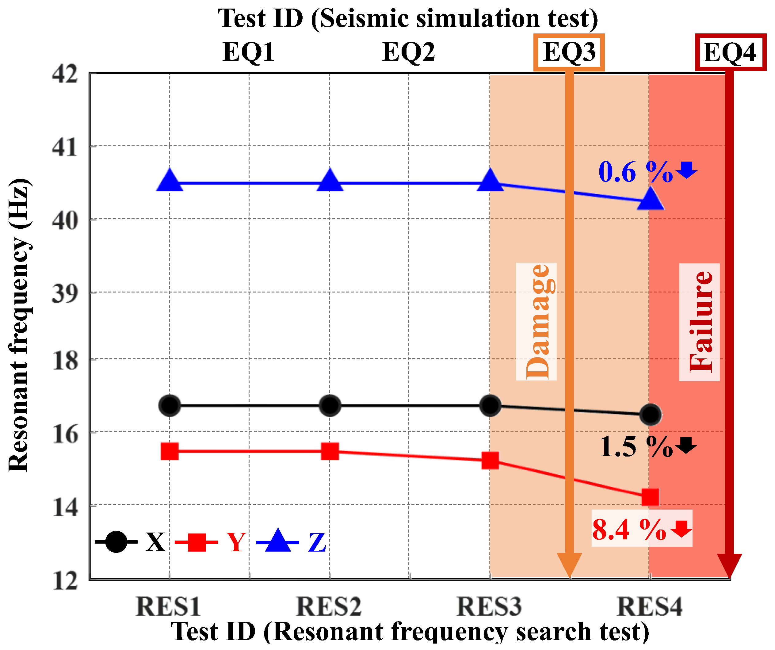
| Test ID | Resonant Frequency (Hz) | Remarks (Visual Inspection) | ||
|---|---|---|---|---|
| Side–Side (X) | Front–Back (Y) | Vertical (Z) | ||
| RES1 | 16.75 | 15.50 | 40.50 | - |
| EQ1 (100%) | - | - | ||
| RES2 | 16.75 | 15.50 | 40.50 | - |
| EQ2 (200%) | - | - | ||
| RES3 | 16.75 | 15.25 | 40.50 | - |
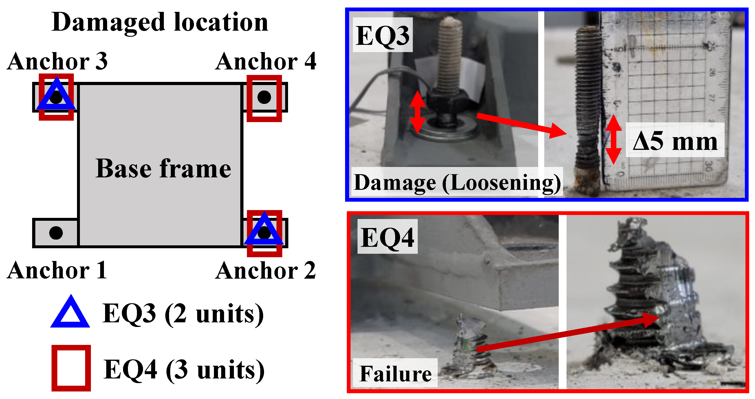
| EQ3 (300%) | - | - Damage to anchor bolts due to plastic deformation (2 units) | ||
| RES4 | 16.50 | 14.25 | 40.25 | - |
| EQ4 (350%) | - | - Failure of anchor bolts (3 units) - Termination of the test | ||
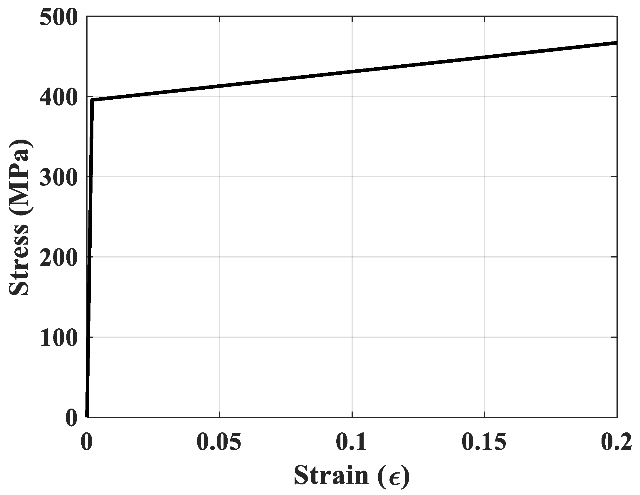
| Density (ton/mm3) | Young’s Modulus (MPa) | Poisson’s Ratio | Yield Stress (MPa) | Plastic Strain |
|---|---|---|---|---|
| 7.85 × 10⁻⁹ | 210,000 | 0.3 | 395.69 | 0 |
| 467.00 | 0.198 |
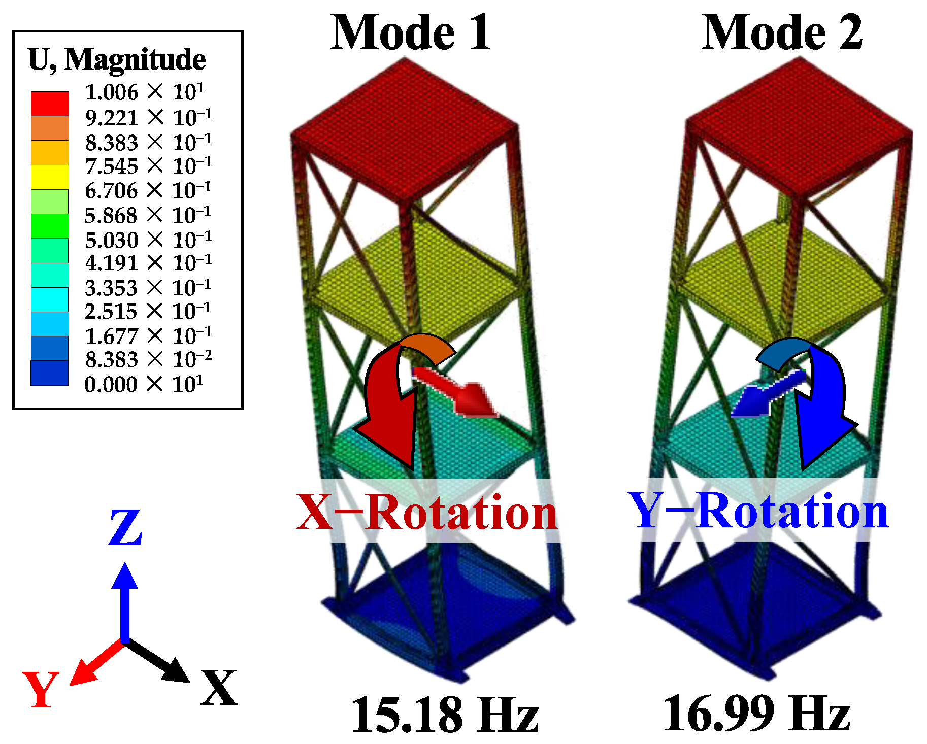
| Mode | Translation | Rotation | ||||
|---|---|---|---|---|---|---|
| X | Y | Z | X | Y | Z | |
| 1 | 0.002 | 0.855 | 0.000 | 0.969 | 0.000 | 0.403 |
| 2 | 0.951 | 0.001 | 0.000 | 0.000 | 0.970 | 0.334 |
| Type | Mode 1 (Y) | Mode 2 (X) | Weight (kg) | |
|---|---|---|---|---|
| Specimen | Resonant frequency (Hz) | 15.50 | 16.75 | 410.00 |
| Numerical model | Natural frequency (Hz) | 15.18 | 16.99 | 410.73 |
| PD (%) | 2.12 | 1.43 | 0.18 | |
| Location | Direction | Test ID | ||
|---|---|---|---|---|
| EQ1 | EQ2 | EQ3 | ||
| A2 | X | 0.975 | 0.957 | 0.811 |
| Y | 0.978 | 0.973 | 0.832 | |
| Z | 0.675 | 0.761 | 0.605 | |
| A3 | X | 0.945 | 0.906 | 0.722 |
| Y | 0.963 | 0.951 | 0.737 | |
| Z | 0.726 | 0.801 | 0.549 | |
| A4 | X | 0.912 | 0.855 | 0.638 |
| Y | 0.950 | 0.936 | 0.725 | |
| Z | 0.717 | 0.785 | 0.506 | |
| Type | Location | EQ1 | EQ2 | EQ3 | |||||||
|---|---|---|---|---|---|---|---|---|---|---|---|
| X | Y | Z | X | Y | Z | X | Y | Z | |||
| A1 | 0.160 | 0.153 | 0.114 | 0.314 | 0.303 | 0.249 | 0.455 | 0.439 | 0.382 | ||
| RMS (g) | Test | A2 | 0.205 | 0.207 | 0.136 | 0.406 | 0.421 | 0.261 | 0.716 | 0.763 | 0.498 |
| A3 | 0.254 | 0.268 | 0.132 | 0.517 | 0.559 | 0.258 | 1.002 | 1.174 | 0.583 | ||
| A4 | 0.302 | 0.323 | 0.133 | 0.631 | 0.692 | 0.267 | 1.328 | 1.501 | 0.620 | ||
| Analysis | A2 | 0.206 | 0.200 | 0.144 | 0.415 | 0.405 | 0.300 | 0.604 | 0.593 | 0.453 | |
| A3 | 0.241 | 0.261 | 0.132 | 0.480 | 0.527 | 0.274 | 0.699 | 0.776 | 0.412 | ||
| A4 | 0.275 | 0.319 | 0.133 | 0.545 | 0.642 | 0.273 | 0.797 | 0.950 | 0.408 | ||
| RRMS (g/g) | Test | A2 | 1.289 | 1.307 | 1.260 | 1.323 | 1.337 | 1.205 | 1.329 | 1.352 | 1.188 |
| A3 | 1.507 | 1.705 | 1.153 | 1.529 | 1.740 | 1.100 | 1.536 | 1.767 | 1.079 | ||
| A4 | 1.716 | 2.080 | 1.159 | 1.738 | 2.122 | 1.095 | 1.752 | 2.165 | 1.068 | ||
| Analysis | A2 | 1.278 | 1.352 | 1.187 | 1.296 | 1.391 | 1.047 | 1.574 | 1.738 | 1.304 | |
| A3 | 1.584 | 1.747 | 1.152 | 1.649 | 1.848 | 1.036 | 2.201 | 2.673 | 1.526 | ||
| A4 | 1.885 | 2.112 | 1.162 | 2.010 | 2.286 | 1.072 | 2.919 | 3.419 | 1.625 | ||
| PD (%) | A2 | 0.84 | 3.38 | 5.98 | 2.08 | 3.94 | 14.03 | 16.91 | 25.01 | 9.32 | |
| A3 | 4.97 | 2.41 | 0.08 | 7.54 | 6.02 | 5.94 | 35.63 | 40.84 | 34.29 | ||
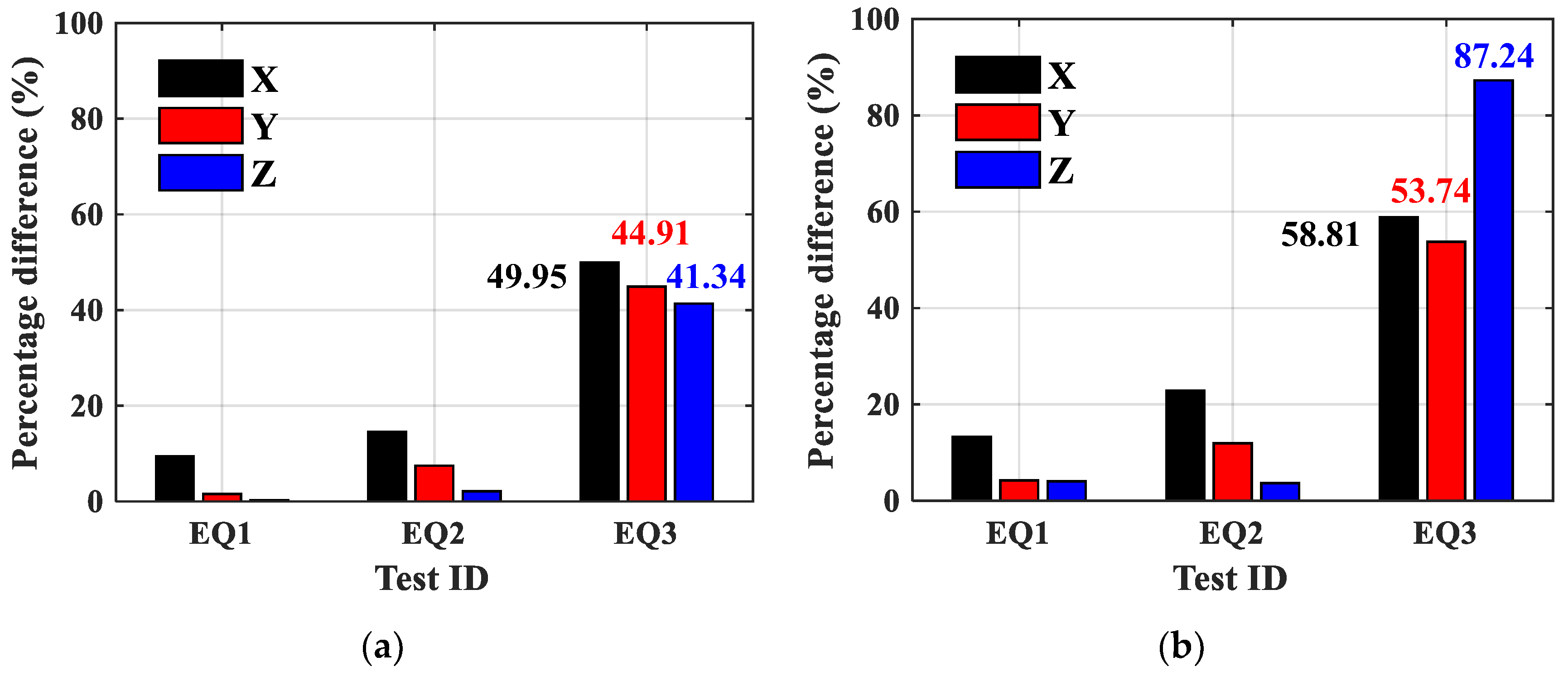
| A4 | 9.39 | 1.55 | 0.25 | 14.52 | 7.47 | 2.14 | 49.95 | 44.91 | 41.34 | ||
| Type | Location | EQ1 | EQ2 | EQ3 | |||||||
|---|---|---|---|---|---|---|---|---|---|---|---|
| X | Y | Z | X | Y | Z | X | Y | Z | |||
| A1 | 0.224 | 0.214 | 0.160 | 0.442 | 0.423 | 0.356 | 0.644 | 0.615 | 0.547 | ||
| RMQ (g) | Test | A2 | 0.286 | 0.288 | 0.188 | 0.575 | 0.584 | 0.371 | 1.036 | 1.084 | 1.351 |
| A3 | 0.352 | 0.372 | 0.183 | 0.737 | 0.777 | 0.368 | 1.456 | 1.798 | 1.346 | ||
| A4 | 0.419 | 0.450 | 0.184 | 0.908 | 0.966 | 0.378 | 1.940 | 2.210 | 1.512 | ||
| Analysis | A2 | 0.275 | 0.274 | 0.212 | 0.550 | 0.543 | 0.452 | 0.800 | 0.797 | 0.702 | |
| A3 | 0.322 | 0.355 | 0.189 | 0.634 | 0.705 | 0.394 | 0.925 | 1.039 | 0.605 | ||
| A4 | 0.367 | 0.431 | 0.192 | 0.722 | 0.857 | 0.392 | 1.058 | 1.274 | 0.593 | ||
| RRMQ (g/g) | Test | A2 | 1.227 | 1.279 | 1.327 | 1.243 | 1.286 | 1.269 | 1.242 | 1.296 | 1.283 |
| A3 | 1.433 | 1.658 | 1.185 | 1.433 | 1.666 | 1.106 | 1.435 | 1.691 | 1.106 | ||
| A4 | 1.633 | 2.014 | 1.201 | 1.633 | 2.027 | 1.101 | 1.643 | 2.072 | 1.085 | ||
| Analysis | A2 | 1.273 | 1.348 | 1.175 | 1.301 | 1.381 | 1.040 | 1.607 | 1.762 | 2.470 | |
| A3 | 1.567 | 1.740 | 1.147 | 1.666 | 1.838 | 1.032 | 2.260 | 2.924 | 2.461 | ||
| A4 | 1.865 | 2.102 | 1.153 | 2.054 | 2.284 | 1.062 | 3.011 | 3.594 | 2.763 | ||
| PD (%) | A2 | 3.73 | 5.27 | 12.10 | 4.53 | 7.16 | 19.82 | 25.65 | 30.49 | 63.28 | |
| A3 | 8.89 | 4.84 | 3.21 | 15.04 | 9.79 | 6.91 | 44.67 | 53.44 | 75.99 | ||
| A4 | 13.23 | 4.25 | 4.02 | 22.82 | 11.96 | 3.65 | 58.81 | 53.74 | 87.24 | ||
| Type | Direction | EQ1 | EQ2 | EQ3 | ||||||||
|---|---|---|---|---|---|---|---|---|---|---|---|---|
| 1–10 Hz | 10–20 Hz | 20–50 Hz | 1–10 Hz | 10–20 Hz | 20–50 Hz | 1–10 Hz | 10–20 Hz | 20–50 Hz | ||||
| A1 | X | 1.020 | 1.561 | 0.704 | 2.047 | 3.145 | 1.443 | 3.040 | 4.568 | 2.269 | ||
| Y | 1.040 | 1.557 | 0.658 | 2.113 | 3.014 | 1.390 | 3.129 | 4.474 | 2.177 | |||
| Z | 0.722 | 1.259 | 0.640 | 1.501 | 2.758 | 1.589 | 2.305 | 4.571 | 2.635 | |||
| Average (g) | Test | A2 | X | 1.114 | 2.409 | 0.955 | 2.253 | 5.351 | 2.215 | 3.425 | 9.141 | 5.196 |
| Y | 1.139 | 2.575 | 0.943 | 2.309 | 5.582 | 2.117 | 3.465 | 10.580 | 5.240 | |||
| Z | 0.727 | 1.637 | 0.785 | 1.503 | 3.291 | 1.707 | 2.318 | 6.509 | 7.264 | |||
| A3 | X | 1.191 | 3.424 | 1.224 | 2.390 | 8.275 | 3.048 | 3.759 | 14.642 | 7.078 | ||
| Y | 1.234 | 3.620 | 1.267 | 2.504 | 8.459 | 3.248 | 3.890 | 17.640 | 8.846 | |||
| Z | 0.722 | 1.606 | 0.772 | 1.486 | 3.274 | 1.886 | 2.367 | 6.269 | 5.521 | |||
| A4 | X | 1.262 | 4.422 | 1.504 | 2.580 | 11.012 | 4.061 | 4.072 | 20.477 | 10.061 | ||
| Y | 1.302 | 4.584 | 1.564 | 2.647 | 11.156 | 4.246 | 4.303 | 23.979 | 10.976 | |||
| Z | 0.716 | 1.617 | 0.794 | 1.503 | 3.441 | 1.907 | 2.355 | 6.369 | 6.726 | |||
| Analysis | A2 | X | 1.036 | 1.775 | 0.842 | 2.082 | 3.549 | 1.734 | 3.113 | 5.272 | 2.402 | |
| Y | 1.083 | 2.143 | 0.794 | 2.175 | 4.113 | 1.570 | 3.246 | 6.149 | 2.432 | |||
| Z | 0.728 | 1.419 | 1.115 | 1.599 | 3.087 | 2.240 | 2.312 | 4.731 | 3.764 | |||
| A3 | X | 1.109 | 2.261 | 0.940 | 2.211 | 4.400 | 1.797 | 3.314 | 6.706 | 2.756 | ||
| Y | 1.178 | 3.009 | 1.020 | 2.378 | 5.854 | 1.983 | 3.539 | 9.036 | 3.166 | |||
| Z | 0.720 | 1.289 | 0.857 | 1.518 | 2.872 | 1.703 | 2.258 | 4.512 | 3.248 | |||
| A4 | X | 1.176 | 2.683 | 1.058 | 2.361 | 5.233 | 2.169 | 3.485 | 8.105 | 3.362 | ||
| Y | 1.257 | 3.770 | 1.259 | 2.534 | 7.540 | 2.409 | 3.791 | 11.668 | 4.007 | |||
| Z | 0.727 | 1.340 | 0.810 | 1.493 | 2.906 | 1.701 | 2.279 | 4.513 | 3.075 | |||
| RAvg (g/g) | Test | A2 | X | 1.092 | 1.543 | 1.356 | 1.101 | 1.701 | 1.534 | 1.126 | 2.001 | 2.290 |
| Y | 1.095 | 1.654 | 1.432 | 1.093 | 1.852 | 1.523 | 1.107 | 2.365 | 2.407 | |||
| Z | 1.007 | 1.300 | 1.225 | 1.002 | 1.193 | 1.074 | 1.006 | 1.424 | 2.757 | |||
| A3 | X | 1.169 | 2.194 | 1.737 | 1.168 | 2.631 | 2.112 | 1.236 | 3.205 | 3.119 | ||
| Y | 1.186 | 2.325 | 1.925 | 1.185 | 2.807 | 2.337 | 1.243 | 3.943 | 4.063 | |||
| Z | 1.001 | 1.275 | 1.206 | 0.990 | 1.187 | 1.187 | 1.027 | 1.371 | 2.095 | |||
| A4 | X | 1.238 | 2.833 | 2.135 | 1.261 | 3.501 | 2.813 | 1.340 | 4.482 | 4.433 | ||
| Y | 1.252 | 2.944 | 2.376 | 1.253 | 3.701 | 3.055 | 1.375 | 5.359 | 5.041 | |||
| Z | 0.992 | 1.284 | 1.241 | 1.001 | 1.248 | 1.200 | 1.022 | 1.393 | 2.553 | |||
| Analysis | A2 | X | 1.016 | 1.137 | 1.196 | 1.017 | 1.128 | 1.201 | 1.024 | 1.154 | 1.059 | |
| Y | 1.041 | 1.376 | 1.206 | 1.029 | 1.365 | 1.129 | 1.037 | 1.374 | 1.117 | |||
| Z | 1.008 | 1.127 | 1.742 | 1.066 | 1.119 | 1.410 | 1.003 | 1.035 | 1.428 | |||
| A3 | X | 1.088 | 1.449 | 1.335 | 1.080 | 1.399 | 1.245 | 1.090 | 1.468 | 1.214 | ||
| Y | 1.133 | 1.933 | 1.549 | 1.125 | 1.942 | 1.427 | 1.131 | 2.020 | 1.454 | |||
| Z | 0.998 | 1.023 | 1.338 | 1.011 | 1.042 | 1.072 | 0.979 | 0.987 | 1.233 | |||
| A4 | X | 1.154 | 1.719 | 1.502 | 1.153 | 1.664 | 1.503 | 1.146 | 1.774 | 1.481 | ||
| Y | 1.209 | 2.421 | 1.912 | 1.199 | 2.502 | 1.734 | 1.212 | 2.608 | 1.841 | |||
| Z | 1.007 | 1.064 | 1.265 | 0.995 | 1.054 | 1.070 | 0.988 | 0.987 | 1.167 | |||
| PD (%) | A2 | X | 7.24 | 30.28 | 12.55 | 7.87 | 40.49 | 24.35 | 9.53 | 53.68 | 73.53 | |
| Y | 5.10 | 18.30 | 17.14 | 5.99 | 30.30 | 29.70 | 6.53 | 52.97 | 73.20 | |||
| Z | 0.17 | 14.26 | 34.81 | 6.22 | 6.40 | 27.03 | 0.27 | 31.62 | 63.48 | |||
| A3 | X | 7.16 | 40.90 | 26.19 | 7.76 | 61.13 | 51.63 | 12.59 | 74.35 | 87.91 | ||
| Y | 4.62 | 18.42 | 21.65 | 5.17 | 36.39 | 48.33 | 9.47 | 64.51 | 94.59 | |||
| Z | 0.27 | 21.91 | 10.40 | 2.12 | 13.07 | 10.16 | 4.71 | 32.60 | 51.84 | |||
| A4 | X | 7.02 | 48.95 | 34.79 | 8.87 | 71.14 | 60.74 | 15.55 | 86.57 | 99.82 | ||
| Y | 3.48 | 19.48 | 21.65 | 4.34 | 38.69 | 55.19 | 12.64 | 69.07 | 93.01 | |||
| Z | 1.41 | 18.77 | 1.95 | 0.69 | 16.86 | 11.43 | 3.29 | 34.11 | 74.50 | |||
| Type | Direction | EQ1 | EQ2 | EQ3 | ||||||||
|---|---|---|---|---|---|---|---|---|---|---|---|---|
| 1–10 Hz | 10–20 Hz | 20–50 Hz | 1–10 Hz | 10–20 Hz | 20–50 Hz | 1–10 Hz | 10–20 Hz | 20–50 Hz | ||||
| A1 | X | 1.020 | 1.561 | 0.704 | 2.047 | 3.145 | 1.443 | 3.040 | 4.568 | 2.269 | ||
| Y | 1.040 | 1.557 | 0.658 | 2.113 | 3.014 | 1.390 | 3.129 | 4.474 | 2.177 | |||
| Z | 0.722 | 1.259 | 0.640 | 1.501 | 2.758 | 1.589 | 2.305 | 4.571 | 2.635 | |||
| Peak (g) | Test | A2 | X | 1.114 | 2.409 | 0.955 | 2.253 | 5.351 | 2.215 | 3.425 | 9.141 | 5.196 |
| Y | 1.139 | 2.575 | 0.943 | 2.309 | 5.582 | 2.117 | 3.465 | 10.580 | 5.240 | |||
| Z | 0.727 | 1.637 | 0.785 | 1.503 | 3.291 | 1.707 | 2.318 | 6.509 | 7.264 | |||
| A3 | X | 1.191 | 3.424 | 1.224 | 2.390 | 8.275 | 3.048 | 3.759 | 14.642 | 7.078 | ||
| Y | 1.234 | 3.620 | 1.267 | 2.504 | 8.459 | 3.248 | 3.890 | 17.640 | 8.846 | |||
| Z | 0.722 | 1.606 | 0.772 | 1.486 | 3.274 | 1.886 | 2.367 | 6.269 | 5.521 | |||
| A4 | X | 1.262 | 4.422 | 1.504 | 2.580 | 11.012 | 4.061 | 4.072 | 20.477 | 10.061 | ||
| Y | 1.302 | 4.584 | 1.564 | 2.647 | 11.156 | 4.246 | 4.303 | 23.979 | 10.976 | |||
| Z | 0.716 | 1.617 | 0.794 | 1.503 | 3.441 | 1.907 | 2.355 | 6.369 | 6.726 | |||
| Analysis | A2 | X | 1.036 | 1.775 | 0.842 | 2.082 | 3.549 | 1.734 | 3.113 | 5.272 | 2.402 | |
| Y | 1.083 | 2.143 | 0.794 | 2.175 | 4.113 | 1.570 | 3.246 | 6.149 | 2.432 | |||
| Z | 0.728 | 1.419 | 1.115 | 1.599 | 3.087 | 2.240 | 2.312 | 4.731 | 3.764 | |||
| A3 | X | 1.109 | 2.261 | 0.940 | 2.211 | 4.400 | 1.797 | 3.314 | 6.706 | 2.756 | ||
| Y | 1.178 | 3.009 | 1.020 | 2.378 | 5.854 | 1.983 | 3.539 | 9.036 | 3.166 | |||
| Z | 0.720 | 1.289 | 0.857 | 1.518 | 2.872 | 1.703 | 2.258 | 4.512 | 3.248 | |||
| A4 | X | 1.176 | 2.683 | 1.058 | 2.361 | 5.233 | 2.169 | 3.485 | 8.105 | 3.362 | ||
| Y | 1.257 | 3.770 | 1.259 | 2.534 | 7.540 | 2.409 | 3.791 | 11.668 | 4.007 | |||
| Z | 0.727 | 1.340 | 0.810 | 1.493 | 2.906 | 1.701 | 2.279 | 4.513 | 3.075 | |||
| RAvg (g/g) | Test | A2 | X | 1.092 | 1.543 | 1.356 | 1.101 | 1.701 | 1.534 | 1.126 | 2.001 | 2.290 |
| Y | 1.095 | 1.654 | 1.432 | 1.093 | 1.852 | 1.523 | 1.107 | 2.365 | 2.407 | |||
| Z | 1.007 | 1.300 | 1.225 | 1.002 | 1.193 | 1.074 | 1.006 | 1.424 | 2.757 | |||
| A3 | X | 1.169 | 2.194 | 1.737 | 1.168 | 2.631 | 2.112 | 1.236 | 3.205 | 3.119 | ||
| Y | 1.186 | 2.325 | 1.925 | 1.185 | 2.807 | 2.337 | 1.243 | 3.943 | 4.063 | |||
| Z | 1.001 | 1.275 | 1.206 | 0.990 | 1.187 | 1.187 | 1.027 | 1.371 | 2.095 | |||
| A4 | X | 1.238 | 2.833 | 2.135 | 1.261 | 3.501 | 2.813 | 1.340 | 4.482 | 4.433 | ||
| Y | 1.252 | 2.944 | 2.376 | 1.253 | 3.701 | 3.055 | 1.375 | 5.359 | 5.041 | |||
| Z | 0.992 | 1.284 | 1.241 | 1.001 | 1.248 | 1.200 | 1.022 | 1.393 | 2.553 | |||
| Analysis | A2 | X | 1.016 | 1.137 | 1.196 | 1.017 | 1.128 | 1.201 | 1.024 | 1.154 | 1.059 | |
| Y | 1.041 | 1.376 | 1.206 | 1.029 | 1.365 | 1.129 | 1.037 | 1.374 | 1.117 | |||
| Z | 1.008 | 1.127 | 1.742 | 1.066 | 1.119 | 1.410 | 1.003 | 1.035 | 1.428 | |||
| A3 | X | 1.088 | 1.449 | 1.335 | 1.080 | 1.399 | 1.245 | 1.090 | 1.468 | 1.214 | ||
| Y | 1.133 | 1.933 | 1.549 | 1.125 | 1.942 | 1.427 | 1.131 | 2.020 | 1.454 | |||
| Z | 0.998 | 1.023 | 1.338 | 1.011 | 1.042 | 1.072 | 0.979 | 0.987 | 1.233 | |||
| A4 | X | 1.154 | 1.719 | 1.502 | 1.153 | 1.664 | 1.503 | 1.146 | 1.774 | 1.481 | ||
| Y | 1.209 | 2.421 | 1.912 | 1.199 | 2.502 | 1.734 | 1.212 | 2.608 | 1.841 | |||
| Z | 1.007 | 1.064 | 1.265 | 0.995 | 1.054 | 1.070 | 0.988 | 0.987 | 1.167 | |||
| PD (%) | A2 | X | 7.24 | 30.28 | 12.55 | 7.87 | 40.49 | 24.35 | 9.53 | 53.68 | 73.53 | |
| Y | 5.10 | 18.30 | 17.14 | 5.99 | 30.30 | 29.70 | 6.53 | 52.97 | 73.20 | |||
| Z | 0.17 | 14.26 | 34.81 | 6.22 | 6.40 | 27.03 | 0.27 | 31.62 | 63.48 | |||
| A3 | X | 7.16 | 40.90 | 26.19 | 7.76 | 61.13 | 51.63 | 12.59 | 74.35 | 87.91 | ||
| Y | 4.62 | 18.42 | 21.65 | 5.17 | 36.39 | 48.33 | 9.47 | 64.51 | 94.59 | |||
| Z | 0.27 | 21.91 | 10.40 | 2.12 | 13.07 | 10.16 | 4.71 | 32.60 | 51.84 | |||
| A4 | X | 7.02 | 48.95 | 34.79 | 8.87 | 71.14 | 60.74 | 15.55 | 86.57 | 99.82 | ||
| Y | 3.48 | 19.48 | 21.65 | 4.34 | 38.69 | 55.19 | 12.64 | 69.07 | 93.01 | |||
| Z | 1.41 | 18.77 | 1.95 | 0.69 | 16.86 | 11.43 | 3.29 | 34.11 | 74.50 | |||
| Type | Location | ZPA (45.25 Hz) | |||||||||
|---|---|---|---|---|---|---|---|---|---|---|---|
| EQ1 | EQ2 | EQ3 | |||||||||
| X | Y | Z | X | Y | Z | X | Y | Z | |||
| A1 | 0.653 | 0.624 | 0.588 | 1.392 | 1.289 | 1.221 | 2.055 | 2.175 | 2.095 | ||
| ZPA (g) | Test | A2 | 0.870 | 0.804 | 0.627 | 2.076 | 1.832 | 1.384 | 7.173 | 5.868 | 9.080 |
| A3 | 1.085 | 1.102 | 0.634 | 2.813 | 2.593 | 1.471 | 8.091 | 10.422 | 7.111 | ||
| A4 | 1.298 | 1.330 | 0.606 | 3.561 | 3.583 | 1.480 | 12.749 | 10.415 | 8.387 | ||
| Analysis | A2 | 0.860 | 0.789 | 1.132 | 1.459 | 1.463 | 1.634 | 2.829 | 2.239 | 3.867 | |
| A3 | 0.866 | 0.919 | 0.831 | 1.567 | 1.726 | 1.567 | 2.373 | 3.023 | 3.836 | ||
| A4 | 0.963 | 1.175 | 0.743 | 1.980 | 2.036 | 1.658 | 2.982 | 3.729 | 3.625 | ||
| RZPA (g/g) | Test | A2 | 1.332 | 1.288 | 1.067 | 1.491 | 1.421 | 1.134 | 3.491 | 2.697 | 4.333 |
| A3 | 1.661 | 1.766 | 1.079 | 2.021 | 2.011 | 1.205 | 3.938 | 4.791 | 3.394 | ||
| A4 | 1.987 | 2.130 | 1.030 | 2.557 | 2.779 | 1.213 | 6.205 | 4.787 | 4.002 | ||
| Analysis | A2 | 1.317 | 1.263 | 1.925 | 1.048 | 1.135 | 1.338 | 1.377 | 1.029 | 1.845 | |
| A3 | 1.327 | 1.473 | 1.413 | 1.125 | 1.339 | 1.283 | 1.155 | 1.390 | 1.830 | ||
| A4 | 1.474 | 1.882 | 1.264 | 1.422 | 1.579 | 1.358 | 1.451 | 1.714 | 1.730 | ||
| PD (%) | A2 | 1.16 | 1.95 | 57.32 | 34.91 | 22.38 | 16.56 | 86.87 | 89.53 | 80.54 | |
| A3 | 22.37 | 18.09 | 26.84 | 56.91 | 40.13 | 6.29 | 109.28 | 110.07 | 59.85 | ||
| A4 | 29.62 | 12.35 | 20.41 | 57.04 | 55.04 | 11.32 | 124.18 | 94.55 | 79.28 | ||
Disclaimer/Publisher’s Note: The statements, opinions and data contained in all publications are solely those of the individual author(s) and contributor(s) and not of MDPI and/or the editor(s). MDPI and/or the editor(s) disclaim responsibility for any injury to people or property resulting from any ideas, methods, instructions or products referred to in the content. |
© 2025 by the authors. Licensee MDPI, Basel, Switzerland. This article is an open access article distributed under the terms and conditions of the Creative Commons Attribution (CC BY) license (https://creativecommons.org/licenses/by/4.0/).
Share and Cite
Yun, D.-W.; Jeon, B.-G.; Kim, S.-W.; Hahm, D.; Lee, H.-P. Comparison of Acceleration Amplification for Seismic Behavior Characteristics Analysis of Electrical Cabinet Model: Experimental and Numerical Study. Appl. Sci. 2025, 15, 7274. https://doi.org/10.3390/app15137274
Yun D-W, Jeon B-G, Kim S-W, Hahm D, Lee H-P. Comparison of Acceleration Amplification for Seismic Behavior Characteristics Analysis of Electrical Cabinet Model: Experimental and Numerical Study. Applied Sciences. 2025; 15(13):7274. https://doi.org/10.3390/app15137274
Chicago/Turabian StyleYun, Da-Woon, Bub-Gyu Jeon, Sung-Wan Kim, Daegi Hahm, and Hong-Pyo Lee. 2025. "Comparison of Acceleration Amplification for Seismic Behavior Characteristics Analysis of Electrical Cabinet Model: Experimental and Numerical Study" Applied Sciences 15, no. 13: 7274. https://doi.org/10.3390/app15137274
APA StyleYun, D.-W., Jeon, B.-G., Kim, S.-W., Hahm, D., & Lee, H.-P. (2025). Comparison of Acceleration Amplification for Seismic Behavior Characteristics Analysis of Electrical Cabinet Model: Experimental and Numerical Study. Applied Sciences, 15(13), 7274. https://doi.org/10.3390/app15137274