Explainable Artificial Intelligence: Advancements and Limitations

Abstract

Explainable artificial intelligence (XAI) has emerged as a crucial field for understanding and interpreting the decisions of complex machine learning models, particularly deep neural networks. This review presents a structured overview of XAI methodologies, encompassing a diverse range of techniques designed to provide explainability at different levels of abstraction. We cover pixel-level explanation strategies such as saliency maps, perturbation-based methods and gradient-based visualisations, as well as concept-based approaches that align model behaviour with human-understandable semantics. Additionally, we touch upon the relevance of XAI in the context of weakly supervised semantic segmentation. By synthesising recent developments, this paper aims to clarify the landscape of XAI methods and offer insights into their comparative utility and role in fostering trustworthy AI systems.

1. Introduction

Deep neural networks (DNNs) have demonstrated impressive predictive performance across various domains, including medicine [1,2], robotics [3,4] and economics [5]. They have been successfully applied to a wide range of problems, such as object detection [6,7], stock prediction [8], image generation [9,10], and machine translation [11,12], among many others. This success can be attributed to advancements in deep learning [13], the availability of massive datasets [14], and the increasing computational power provided by graphics processing units (GPUs) [15].

Despite the significant performance improvements in DNNs over recent years, gaining trust in their predictions remains a challenge due to the complex and opaque nature of their decision-making processes [16,17,18,19,20,21]. To address this, model interpretability has become essential in uncovering the “black box” of deep networks. Interpretability, often defined as the ability to provide explanations in terms understandable to humans [22], plays a crucial role in bridging the gap between DNNs’ performance and user trust. Ongoing discussions have explored the distinctions between terms like interpretability, explainability, trustworthiness, and transparency, debating their appropriate use in the field [18,23,24,25]. In this review, we focus on the shared goal of explainable artificial intelligence (XAI) methodologies—to make AI more understandable to humans—and leave a detailed discussion of the differences among these approaches for future work.

The techniques developed to interpret and explain machine learning (ML) models are broadly categorised as XAI methodologies [26,27]. Consequently, this review adopts XAI as its core term. In recent years, the field of XAI has experienced exponential growth, with numerous approaches proposed to address the transparency challenge of black-box models. These approaches aim to make such models safer for deployment, especially in sensitive domains, including healthcare [28,29] and law [30]. By improving transparency, XAI seeks to achieve several objectives, such as ensuring fairness by detecting and mitigating discrimination or unexpected behaviours in ML systems. XAI techniques also assist practitioners in debugging their systems by identifying biases in data or in the models themselves [20,31]. Furthermore, explainability is not merely a desirable feature; since 2018, the General Data Protection Regulation (GDPR) in Europe has mandated that artificial intelligence (AI) systems provide justifications for their decisions, further underscoring the critical role of XAI [32,33].

There have been a significant number of reviews on XAI focusing on different aspects of this important subfield. These reviews share many common goals, such as the definition of interpretability and its types [16,17]. Some of these reviews specifically focus on the detailed taxonomy of existing methodologies and providing the differences between terms like explainability, interpretability and transparency [18,34]. Some surveys, on the other hand, highlight the importance of explainability in modern technologies, particularly within the application domains of Industry 4.0 [35].

Our main contribution is, however, the definition of the dimensions of XAI, which, to the best of our knowledge, has never been explicitly put together before. We define six main dimensions, where each of them is further divided into two subcategories. We claim that any XAI methodology currently exists or proposed in the future could be put under these categories. Proposed techniques frequently belong to multiple subcategories within these dimensions. For instance, a single method might generate both visual and conceptual explanations or be applicable to both traditional ML models and deep learning architectures. This overlapping nature reflects the versatility and multifaceted nature of XAI techniques, which are not confined to a single category but instead span across several, depending on their design and application.

We analyse the advantages and limitations of a variety of methodologies across these categories. This review is intended to serve both practitioners and researchers: for end users, it provides guidance on selecting the most appropriate XAI technique for their specific use case; for researchers, it highlights current gaps and challenges in the field, potentially inspiring new directions for future work.

We then focus on one specific dimension, i.e., explanation modality, which involves the subcategories visual and conceptual. We argue that the modality of explanations is the most crucial aspect, especially for visual tasks, and the future of explainability depends on the ability of methodologies to provide both visual and conceptual explanations.

Although this review focuses on XAI for architectures processing static data, explaining models such as LSTMs [36], GRUs [37], and Transformers [38] has also become increasingly important as countless real-world applications employ these models for sequential data processing. In this direction, many works have either adapted existing XAI methodologies to temporal data or developed novel ones specifically for them. TimeSHAP [39], for instance, extends KernelSHAP [40] to explain the predictions of recurrent neural networks (RNNs) [41]. Similarly, explainable attention-based methods—e.g., RETAIN [42] or Temporal Fusion Transformer (TFT) [43]— aim to embed interpretability within the model architecture by highlighting key timesteps or variables directly via learned attention weights. Despite these advances, translating dynamic model behaviours into human-centric insights is still a significant challenge for dynamic XAI. In this survey, we do not delve into the dynamic XAI or propose solutions to its challenges, as we reserve this for a separate, more detailed future work.

This paper is structured as follows. Section 2 discusses the black-box nature of convolutional neural networks (CNNs) and provides a brief history of their development. Section 3 introduces the overarching categorisation of XAI methodologies, laying the foundation for the detailed discussions that follow. Visual explanation techniques are covered in Section 4, while concept-based approaches are reviewed in Section 5. In Section 6, we explore the close relationship between XAI and the field of weakly supervised semantic segmentation (WSSS), highlighting key methodologies and their shared objectives. Finally, Section 7 offers concluding remarks and perspectives on future directions.

2. Black-Box Nature of CNNs

First proposed in 1998 for handwritten character recognition [44], CNNs have shown a remarkable performance, especially in vision tasks. Thanks to the ImageNet dataset [14] and efficient GPUs that enabled thousands of computations in parallel, AlexNet by Krizhevsky et al. achieved state-of-the-art performance in ImageNet LSVRC-2012 competition [45]. Following AlexNet, several even more performant architectures have been proposed including but not limited to VGG [46], GoogleNet [47], ResNet [48], DenseNet [49], MobileNet [50], EfficientNet [51], and ConvNeXt [52,53]. With these CNN-based architectures, human-level performance has already been reached and arguably outperformed in various tasks. However, CNNs’ black-box nature has been seen as the main obstacle to their further deployment, especially in fields where human life is at stake.

The so-called black-box nature of CNNs arises from their end-to-end learning process, which contrasts with traditional ML methods such as decision trees [54] and support vector machines (SVMs) [55] where features are manually designed by experts—for example, edge and texture detectors or colour histograms—tailored to specific tasks [56,57]. As the decision process of traditional ML techniques is built around these predefined, human-understood features, it is relatively easy to follow the reasoning behind their predictions. In contrast, CNNs automatically learn features directly from data through multiple layers of abstraction without any human intervention. This automatic feature extraction helps CNNs achieve state-of-the-art performance, but it also complicates our understanding of what the model is learning at each stage. The learned representations are highly complex and the decision process is non-linear, which leads to an opaque decision-making that obscures the internal workings of the model [58].

Several methodologies were proposed to tackle these opaque predictions and make deep networks more transparent. In this direction, efforts to enhance the interpretability of CNNs have focused on two primary strategies: visualising model behaviour and aligning learnt high-level features with human-understandable concepts.

Visualisation techniques aim to illuminate how CNNs build complex representations hierarchically from simpler ones, as early studies revealed that initial layers learn basic features like edges and lines, while later layers capture textures and patterns, culminating in the penultimate layer focusing on object parts—insights contributing to what in [59] is described as Algorithmic Transparency [60,61,62]. Additionally, pixel attribution methods highlight specific regions of input images that most strongly influence model predictions, providing a clearer understanding of what drives specific decisions [63,64].

In contrast, feature–concept alignment methodologies seek to map high-level features learnt by CNNs to human-interpretable concepts [65,66,67]. These approaches reconnect abstract representations of deep networks with predefined, semantically meaningful concepts, akin to the handcrafted features used in traditional models. By doing so, they aim to bridge the gap between the opaque, high-dimensional workings of CNNs and human intuition, making the decision-making process more transparent and understandable.

An ideal XAI methodology would seamlessly address both directions detailed above: it would not only match high-level features automatically extracted during training to human-understandable concepts but also localise these concepts spatially within an examined input sample. Such methodology would provide a more holistic explanation, enabling users to understand not only what the model has learned but also where these concepts are represented in the input. This dual capability would allow for more intuitive and interpretable model explanations, improving trust and transparency in AI systems across various domains.

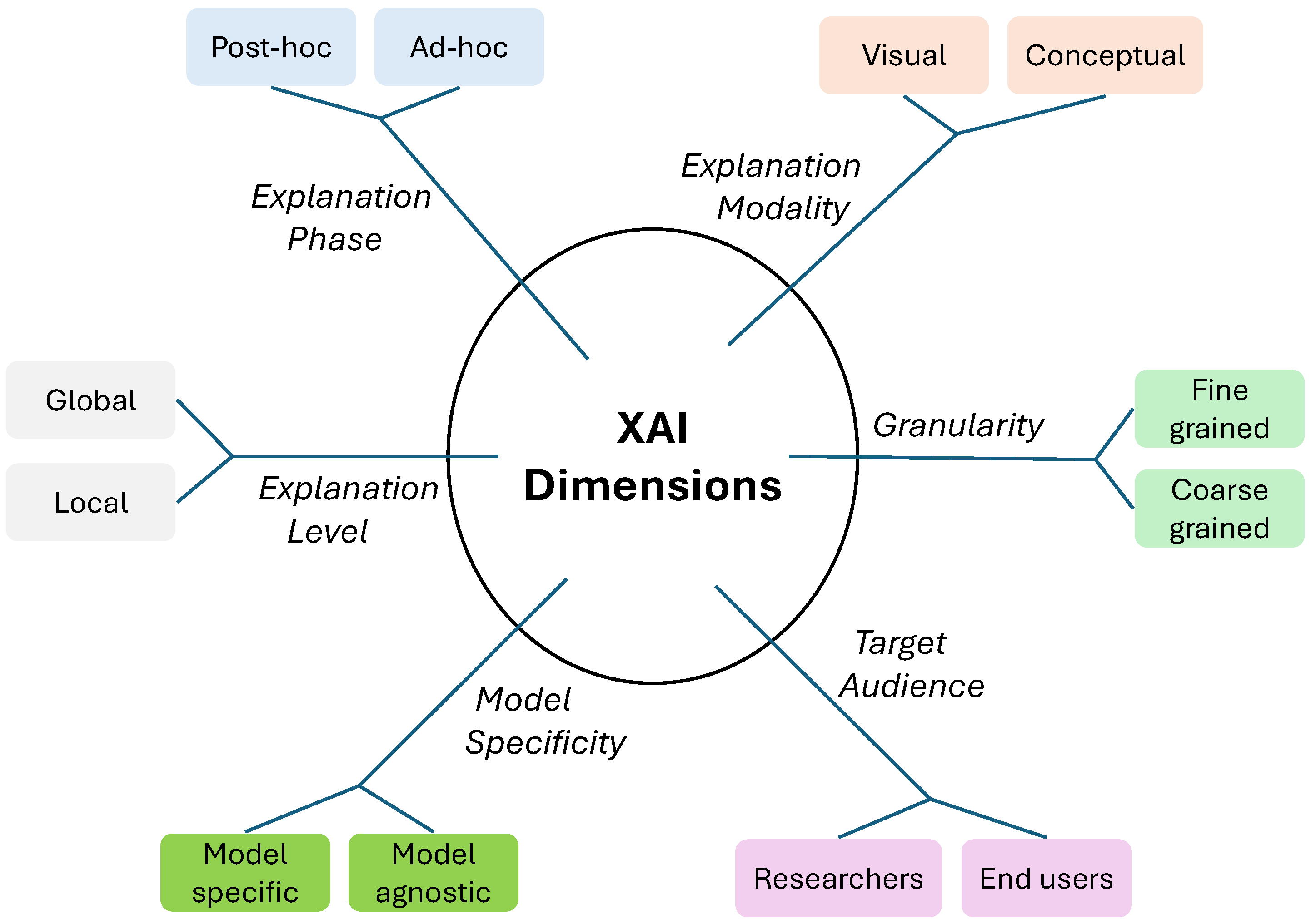
3. Overview of XAI Categorisation: Key Dimensions

This section explores six critical dimensions for categorising XAI methodologies: explanation phase, explanation level, model specificity, target audience, granularity, and modality of explanations. These dimensions provide a structured framework for understanding how XAI techniques differ in their approaches and applications; please also refer to Figure 1 for an overview. Additionally, Table 1 presents the categories of some well-known XAI methodologies along these dimensions, and it can be used as a guide when choosing the right technique for a given task.

Explanation Phase. XAI techniques are typically categorised into two main types: post hoc and ad hoc methods. Post hoc methods are applied after the model has been trained and offer explanations without altering the model structure or any training/test time intervention [63,68]. These methods aim to interpret the decision-making process retrospectively, often using visualisations or perturbation techniques. In contrast, ad hoc methods refer to models that are either inherently interpretable, such as linear models and decision trees, or that incorporate explainability directly into their architecture during training [66,69]. While inherently interpretable methods often have limited predictive capacity, techniques that integrate explainability into black-box models typically experience a performance trade-off due to the structural training/test time interventions. Unlike post hoc methods, which provide explanations after the fact, ad hoc techniques offer immediate by-product interpretability.

Table 1. Categories of some well-known XAI methodologies.

	Category	Phase		Level		Specificity		Audience		Granularity		Modality
Methodology		Post hoc	Ad hoc	Global	Local	Specific	Agnostic	Researchers	End Users	Fine-Grained	Coarse-Grained	Visual	Conceptual
Activation maximisation [61,70,71,72]		✓	✗	✓	✗	✓	✗	✓	✓	✗	✓	✓	✗
Saliency mapping [60,63,73]		✓	✗	✗	✓	✓	✗	✓	✓	✗	✓	✓	✗
Integrated Gradients [74]		✓	✗	✗	✓	✓	✗	✓	✓	✗	✓	✓	✗
Multilevel XAI [75]		✗	✓	✗	✓	✓	✗	✓	✓	✓	✓	✓	✓
CBM [67]		✗	✓	✗	✓	✓	✗	✓	✓	✓	✗	✗	✓
CAM [76]		✓	✗	✗	✓	✓	✗	✓	✗	✗	✓	✓	✗
LIME [77]		✓	✗	✗	✓	✗	✓	✓	✓	✗	✓	✓	✗
Anchors [78]		✓	✗	✗	✓	✗	✓	✓	✓	✗	✓	✓	✗
Network dissection [79]		✓	✗	✓	✗	✓	✗	✓	✓	✓	✓	✓	✓
TCAVs [66]		✓	✗	✓	✗	✓	✗	✓	✓	✓	✗	✗	✓
Post hoc CBM [69]		✓	✗	✓	✗	✓	✗	✓	✓	✓	✗	✗	✓

Table 1. Categories of some well-known XAI methodologies.

	Category	Phase		Level		Specificity		Audience		Granularity		Modality
Methodology		Post hoc	Ad hoc	Global	Local	Specific	Agnostic	Researchers	End Users	Fine-Grained	Coarse-Grained	Visual	Conceptual
Activation maximisation [61,70,71,72]		✓	✗	✓	✗	✓	✗	✓	✓	✗	✓	✓	✗
Saliency mapping [60,63,73]		✓	✗	✗	✓	✓	✗	✓	✓	✗	✓	✓	✗
Integrated Gradients [74]		✓	✗	✗	✓	✓	✗	✓	✓	✗	✓	✓	✗
Multilevel XAI [75]		✗	✓	✗	✓	✓	✗	✓	✓	✓	✓	✓	✓
CBM [67]		✗	✓	✗	✓	✓	✗	✓	✓	✓	✗	✗	✓
CAM [76]		✓	✗	✗	✓	✓	✗	✓	✗	✗	✓	✓	✗
LIME [77]		✓	✗	✗	✓	✗	✓	✓	✓	✗	✓	✓	✗
Anchors [78]		✓	✗	✗	✓	✗	✓	✓	✓	✗	✓	✓	✗
Network dissection [79]		✓	✗	✓	✗	✓	✗	✓	✓	✓	✓	✓	✓
TCAVs [66]		✓	✗	✓	✗	✓	✗	✓	✓	✓	✗	✗	✓
Post hoc CBM [69]		✓	✗	✓	✗	✓	✗	✓	✓	✓	✗	✗	✓

Explanation Level. XAI methods can also be distinguished by whether they provide global or local explanations. Global explanations aim to give a comprehensive view of how a model behaves across a wide range of inputs, offering insight into the overall functioning of the model. Local explanations, in contrast, focus on specific predictions, providing details on why the model makes a certain decision for a particular input. In short, this category highlights the scale at which a model’s behaviour is interpreted, whether explaining its behaviour in general or for individual instances.

Model Specificity. For this aspect, XAI methods are labelled as either model-specific or model-agnostic. Model-specific methods [67,76,80,81] are designed to work with particular types of architectures, such as CNNs, utilising their unique architecture for explanations. Model-agnostic methods [40,66,77,78,82], however, can be applied to any ML model, regardless of its structure, as they only require test inputs and the prediction function. This categorisation reflects the adaptability of XAI techniques, indicating whether they are specialised for certain architectures or can be broadly applied across different models.

Target Audience. XAI methods are designed to cater to different groups of users with varying needs. Some tools are tailored for researchers and developers who require deep insights into model behaviour to refine and improve model architectures. These tools often provide detailed, technical explanations and are useful during model development. On the other hand, there are methods aimed at end users who need to understand model outputs without delving into the underlying technical details. For these users, interactive visualisations or simplified explanations are more appropriate, helping them trust and comprehend a system’s decisions. Google’s what-if tool [83], AI Explainability 360 toolkit by IBM [84], and H₂O AutoML platform [85] are some user-friendly examples.

Granularity. Granularity refers to the level of detail provided by an XAI technique. In this direction, methodologies can be categorised as offering fine-grained or coarse-grained explanations. Fine-grained explanations, such as concept-level insights, delve into more detail of a model’s decisions, offering feature-specific information [75,79]. In contrast, coarse-grained explanations, like class-level or object-level insights, offer a more general understanding of why a model made a particular prediction, typically explaining what contributed to the decision overall [63,68,80]. This category helps determine the level of precision or detail in the explanations, depending on the needs of the user. To give an example, for an animal classification task, a coarse-grained explanation would be a saliency map highlighting the class of interest for a test image, whereas a fine-grained explanation would generate more granular, concept-wise heatmaps highlighting different parts of the object in an input image alongside their textual descriptions.

Modality of Explanations. In this aspect, the distinction lies between the types of generated explanations. For visual tasks, there are two common modalities: visual and conceptual. Visual explanations often involve heatmaps that highlight important regions of an image, giving an intuitive, visual representation of what influenced the model’s decision [40,77]. Conceptual explanations, on the other hand, ideally offer explanations as human-understandable concepts, e.g., stripe for a zebra image [66,67]. In the next sections, we delve deeper into these two modalities, offering more detailed insights and a review of the relevant literature surrounding both modalities. An overview of the next section is also presented in Figure 2. For each modality, we explore key methodologies, drawing on existing research to highlight the strengths and limitations of these approaches. This examination also aims to provide a comprehensive understanding of the role each modality plays in enhancing AI interpretability and trustworthiness.

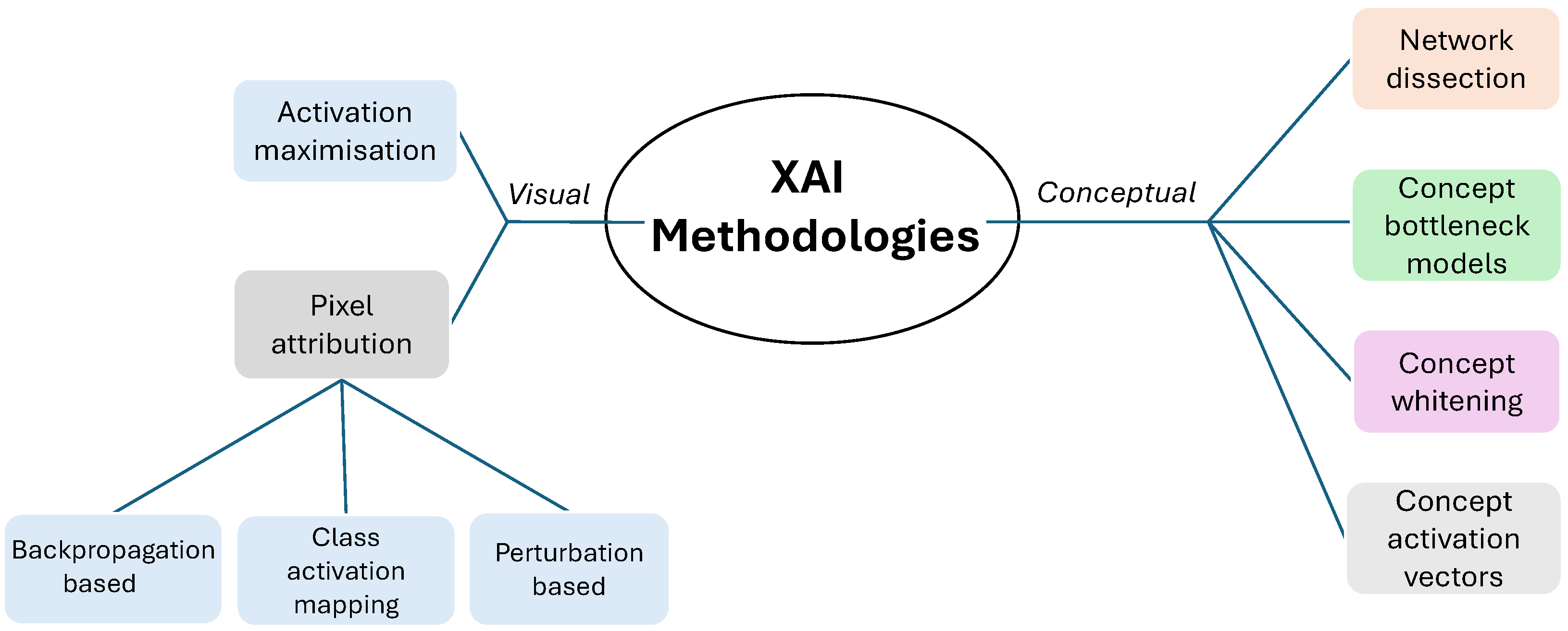
4. Visual Explanations

Visual explanations are arguably the most widely used XAI techniques for computer vision tasks as they offer a direct way to interpret model decisions by providing visual representations of what a model makes its decisions based on. This category encompasses a wide range of methods, often focusing on how particular parts of an image contribute to a model’s output. The goal of visual explanations is to make the inner workings of deep networks, especially CNNs, more transparent and interpretable.

4.1. Activation Maximisation

Visual explanations for CNN decisions can take the form of patterns that strongly activate a neuron, a feature map, an entire layer, or a predicted class—a process commonly referred to as activation maximisation. A notable methodology in this direction is random noise image optimisation. This approach starts with a random noise image, and the gradients of a specific unit are computed with respect to this image. The process identifies the patterns that most strongly activate the targeted unit, resulting in visionary pattern images that offer insights into the network’s learnt representations [61,70,71,72]. Activation maximisation with random image optimisation, while useful for understanding which input patterns maximise the response of specific neurons or layers in black-box models, comes with several limitations. One significant drawback is that the generated visualisations often lack interpretability and clarity, especially for higher-level neurons. The images produced tend to be highly abstract and sometimes visually unrealistic, making it difficult for humans to intuitively grasp what the model is focusing on. Additionally, they require numerous optimisation steps to generate meaningful activations, which makes them computationally expensive and hence their real-time or large-scale applications challenging.

An alternative approach, which eliminates these drawbacks, outputs real images instead. This is achieved by feeding the entire training set to the trained model and selecting a group of images that highly activate a specific unit [61,86]. However, this approach places a significant burden on end users, who must manually sift through highly activating images to identify common patterns—a process that is highly susceptible to human bias.

In addition to the mentioned drawbacks, activation maximisation techniques are also prone to adversarial artefacts—small changes in the input can drastically change the output activation without corresponding to any meaningful difference in the input image, undermining the reliability of the explanations. Overall, while activation maximisation offers insights into model behaviour, its limitations in clarity, computational cost, and susceptibility to noise reduce its practical utility in explainability.

4.2. Pixel Attribution

Pixel attribution techniques aim to find out image parts that contribute to their class predictions the most by creating heatmaps. These maps are used to mask input images to highlight specific parts crucial for a specific prediction. A heatmap is obtained by assigning an importance score to each pixel or a group of pixels. The intuition behind pixel attribution draws from the principles of linear models. In the case of a simple linear model where an input $\mathit{x}={(x^{\left(1\right)},\dots ,x^{\left(P\right)})}^{\top }$ with P features is classified by, say, a single neuron without any non-linear activation, the class score for a particular class c is computed as $S_c={\sum }_i{w}_c^{\left(i\right)}{x}^{\left(i\right)}$, where ${\mathit{w}}_c={(w_c^{\left(1\right)},\dots ,w_c^{\left(P\right)})}^{\top }$ is a weight vector. This intuitively means that each feature in $\mathit{x}$ contributes to the overall score based on its corresponding weight in ${\mathit{w}}_c$. A feature with a higher score, i.e., $w_c^{\left(i\right)}\ast x^{\left(i\right)}$, has a greater impact on the class score, as $S_c$ is a weighted sum of the feature values. Thus, features with higher values after being multiplied by their corresponding weights are considered more important in determining the class prediction. This simple idea is the foundation of pixel attribution methodologies which assign a score to each pixel in an input image based on its contribution to the class prediction.

We can adapt the linear example above to a more complex image classification scenario achieved by CNNs. We let $\mathit{x}\in {\mathbb{R}}^P$ denote an input image with P pixels to be classified as one of the C classes. A trained model defines a mapping function $f:{\mathbb{R}}^P\to {\mathbb{R}}^C$, which generates a probability vector expressed as $g\left(\mathit{x}\right)=[S_1,\dots ,S_C]$, where $S_c$ represents the probability score for class c. Attribution methods assign a relevance score to each pixel in $\mathit{x}$, denoted as ${\mathit{r}}_c=[r_c^{\left(1\right)},\dots ,r_c^{\left(P\right)}]$, where $r_c^{\left(i\right)}$ represents the relevance score of pixel i for class c. Obtaining these relevance scores helps us mask the input image accordingly and derive a saliency map [59]. As CNNs are complex architectures and include multiple layers with nonlinearities, the linear approach cannot be directly applied, i.e., obtaining ${\mathit{r}}_c$ is not as straightforward as ${\mathit{w}}_c$. However, various approximations have been proposed as detailed below.

4.2.1. Backpropagation-Based Saliency Mapping

Backpropagation-based methods are widely used for saliency mapping [60,63,73]. In this direction, Simonyan et al. presented the first saliency mapping technique where they take gradients of a class score $S_c$ for class c with respect to the pixels of the input image $\mathit{x}$ [63]. These gradients result in a relevance score vector, ${\mathit{r}}_c={\displaystyle \frac{\partial S_c}{\partial \mathit{x}}}$, with the same size as the input image. Higher positive relevance scores indicate important pixels for class c, while lower ones show insignificance. In addition, high negative values can be seen as an indicator of other classes or backgrounds. These relevance scores then can be used to weigh the pixels to create a saliency map [59,63]. As Springenberg et al. presented, the other two well-known gradients-based methods, deconvolution [60,87] and guided backpropagation, indeed follow the same process as Simonyan’s approach apart from the way they backpropagate through the activation functions [73].

Integrated Gradients [74] provides a principled way to quantify the contribution of each input feature to a model’s prediction. It addresses some of the limitations of the early gradient-based methods, which can be noisy or misleading due to local irregularities in the model’s gradients. They compute attributions by integrating the gradients of the model’s output with respect to the input along a straight path from a baseline (e.g., a black image or zero vector) to the actual input. Mathematically, it averages these gradients over multiple steps along the path, ensuring that the attributions are both robust and meaningful. The author claims that their approach satisfies desirable theoretical properties, such as completeness, which ensures that the sum of all attributions matches the difference between the model output for the input and the baseline. By providing a clear and interpretable mapping of input features to their contributions, Integrated Gradients has been recognised as an important technique in XAI research.

Deep learning important features (DeepLIFT) [88] is another backpropagation-based pixel attribution method that provides a robust framework for explaining the predictions of deep networks by comparing the activations of neurons to their reference activations. Unlike gradient-based methods, which can suffer from issues such as vanishing gradients or noise, DeepLIFT assigns contribution scores by tracking the changes in outputs relative to a baseline input. It propagates these contributions backwards through the network using a set of predefined rules to ensure consistency and efficiency. The key innovation of DeepLIFT lies in its ability to handle nonlinearities more effectively by considering both the input and the reference, allowing it to capture meaningful attributions even in complex networks. DeepLIFT is also claimed to satisfy the completeness property (the sum of attributions matches the difference between the model output for the input and the baseline) similar to the Integrated Gradients approach. In addition, it also holds the symmetry (equal changes in symmetric inputs receive equal attributions) property which contributes to their robustness and safe use.

LRP (layer-wise relevance propagation) [68,89,90,91] is a powerful explainability technique designed to interpret the decisions of DNNs by tracing back the contributions of individual input features to the model’s output. LRP works by decomposing the prediction score and redistributing it layer by layer, from the output back to the input, using a set of conservation rules. This redistribution ensures that the total relevance is preserved at each layer, ultimately assigning relevance scores to input features in a way that reflects their contribution to the prediction. By doing so, LRP is claimed to satisfy important properties such as relevance conservation and provides insights into how specific features, such as pixels in an image, influence the model’s output.

Backpropagation-based XAI methodologies have been pivotal in unravelling the inner workings of complex neural networks. They offer a relatively efficient way to link input features to model predictions, enabling practitioners to gain insights into model behaviour and hence increase trustworthiness. These methods are particularly appealing due to their simplicity and adaptability across various neural architectures. However, their limitations are equally noteworthy. One key issue is their lack of precision, as they often produce coarse, blurry visualisations that highlight large, indistinct regions of the image, making it difficult to pinpoint exactly what features the model is focusing on. This can be particularly problematic when interpreting decisions in tasks like medical imaging or autonomous driving, where fine-grained details are critical. These methodologies also often suffer from instability and lack of robustness, with explanations being sensitive to minor input perturbations. They may also struggle to capture global model behaviour, instead focusing on local feature importance, which can lead to misleading or incomplete interpretations. Furthermore, the ones that employ gradients may be vulnerable to vanishing gradients and susceptible to noise. Additionally, saliency maps by backpropagation-based methodologies tend to be post hoc explanations, meaning they provide insights only after a decision is made, which might not always reflect the true reasoning process of the model.

In summary, these shortcomings reduce the effectiveness of backpropagation-based methodologies in providing clear, consistent, and trustworthy interpretations, especially in high-stakes applications, which underline the need for complementary XAI approaches that provide more consistent and comprehensive explanations.

4.2.2. Class Activation Mapping (CAM)

Another group of methods, CAM, leverage the final convolutional layer of DNNs, which is shown to capture the most meaningful and complete object signals [62]. Unlike backpropagation-based approaches, CAM focuses on high-level features within these layers rather than tracing gradients or activations back to the input pixels. The first CAM method, introduced by Zhou et al., was designed for architectures incorporating a global average pooling (GAP) layer between the final convolutional and classification layers [76]. In this method, the GAP layer computes a scalar value $F^k$ for each feature map ${\mathit{f}}^k$, which is then passed to the classification layer along with weights $\mathit{w}$ for $k=1,\dots ,K$. The class score for a particular class c is calculated as $S_c=\sum w_c^k{F}^k$, where $w_c^k$ denotes the contribution of $F^k$—and by extension, the feature map ${\mathit{f}}^k$—to the score for class c. Each feature map ${\mathit{f}}^k$ in the final convolutional layer, prior to the GAP operation, is expected to highlight the region that corresponds to the concept it represents when scaled by its calculated weight $w_c^k$.

For instance, in a face recognition task, a feature map activated by the nose might receive a high weight, while one responding to unrelated features, such as a car wheel, would be assigned a low or even negative weight. The weighted sum of these feature maps is then upsampled to the input image’s resolution, producing a saliency map that highlights the most relevant regions for the examined class.

A key limitation of the CAM approach is that it can only be applied to CNNs with a GAP layer between the last convolutional and classification layers, such as GoogleNet [47]. For architectures lacking this structure, CAM requires modifying the model by adding a GAP layer after the final convolutional layer. However, this alteration necessitates model retraining, which can lead to performance degradation compared to the original model.

GradCAM [80] was introduced to overcome the limitations of CAM, particularly its dependency on GAP and successfully used in case studies such as in [92]. As a generalisation of CAM, GradCAM eliminates the need for specific model types or architectural modifications, making it more versatile and broadly applicable. This is achieved thanks to the way GradCAM weighs each feature map; differently from CAM, it takes the gradients of the output score $S_c$ for a given class c with respect to each feature map ${\mathit{f}}^k$ at the last convolutional layer, i.e., ${\displaystyle \frac{\partial S_c}{\partial {\mathit{f}}^k}},k=1,\dots ,K$. After this process, K different gradient maps are obtained. Finally, by applying GAP, a single weight

$$w_c^k={\displaystyle \frac{1}{Z}}\sum _i{\displaystyle \frac{\partial S_c}{\partial f_i^k}}$$

(1)

for each feature map is obtained, where i indicates the location of each pixel and Z is the total number of pixels in the feature map ${\mathit{f}}^k$. Following that, similar to CAM, a weighted sum of the feature maps generates a heatmap with the same dimensions as ${\mathit{f}}^k$; also, see Figure 3 for an illustration. ReLU is also applied to keep features that positively affect a given class and ignore the negative signals that probably are for the other classes. Lastly, acquired heatmaps are upsampled to the size of the input image to highlight important parts of it. In addition, the authors showed how to obtain more class-discriminative and fine-grained results using simple element-wise multiplication between saliency maps generated with GradCAM and guided backpropagation [73].

More approaches were proposed to further refine the resulting activation maps of GradCAM. For instance, Chattopadhay et al. proposed the GradCAM++ method to generate better localisation and handle multiple instances in a single image [93]. The main difference of this approach from GradCAM is taking into account only positive partial derivatives of feature maps at the last convolutional layer. ScoreCAM [64], presented by Wang et al., gets rid of the dependency on gradients of the GradCAM method by masking input images according to feature maps to obtain perturbed images. Scores obtained by forward passes of these images are used as weights, for instance, $w_c^k$ for feature map k. This method claims to reduce noise in the saliency maps caused by gradients.

Advanced CAM methods, including Grad-CAM and Grad-CAM++, have been widely adopted for visualising the important regions of an image that contribute to a model’s decision, but they also come with notable limitations. One key issue is that while they can be applied to a broader range of architectures than traditional CAM (which requires GAP), the visualisations they produce are often still relatively coarse and low-resolution. This can obscure fine details that might be critical in tasks such as medical image analysis or detailed object recognition, where understanding subtle features is essential. Moreover, CAM-based methods generally highlight large regions of an image, making it difficult to differentiate between important and unimportant features within these highlighted areas. Additionally, CAM methods typically focus on explaining a model’s final decision for a specific class, offering little insight into the intermediate layers or the broader decision-making process across the network. This narrow focus limits their ability to provide a holistic understanding of how the model processes and interprets input data. Overall, while CAM methods offer valuable insights, their lack of spatial precision and limited scope reduce their effectiveness in generating deep, fine-grained explanations.

4.2.3. Perturbation-Based Methodologies

Another approach to pixel attribution involves perturbation-based methodologies. These methods use altered versions of an image to gain insights into a model’s inner workings. For example, in the occlusion sensitivity technique by Zeiler et al. [60], a portion of an image is replaced with a patch that contains either the average pixel value of the entire image or a uniform colour. Newly created perturbations are then passed through the trained model to see the effect of the occluded area on the prediction. Despite being as simple as blocking a part of an image, occlusion is shown to be an effective approach. To give an example, the authors showed that when they occlude a dog’s head in a given image, the probability for the dog class drops significantly, which indicates that the head of the dog is crucial for the trained model when making that specific prediction.

In a similar methodology, RISE [82] employs an automated approach to generate perturbations for attribution maps. Given a trained CNN model $f:{\mathbb{R}}^{H\times W}\to {\mathbb{R}}^C$ that maps an input image $\mathit{X}$ of size $H\times W$ to an output class c, RISE introduces a binary mask $\mathit{M}$ sampled from a random distribution and of the same size as $\mathit{X}$. By performing element-wise multiplication of $\mathit{M}$ and $\mathit{X}$, a perturbed image is created with random occlusions at specific pixel locations. Repeating this process with multiple masks produces a set of perturbed images. The model’s prediction probabilities for class c are then computed for each perturbed image and used as weights. Finally, a weighted sum of all perturbed images is used to generate an attribution map. The idea of occluding parts of an image or starting from a blank image and incrementally adding random patches (or pixels) to observe changes in the classification score for a given output class has inspired many model-agnostic methods, which we discuss next.

We now review some well-known model-agnostic methods, which fall under the category of perturbation-based pixel attribution techniques. These methodologies are not designed specifically for CNNs and can be applied to any trained ML model, as they only require the investigated input sample and the prediction function. Often referred to as “black-box” XAI techniques, these methods do not rely on access to the trained model’s internal components, such as weights or feature maps, unlike most of the approaches reviewed so far.

One of the well-known model-agnostic techniques, local interpretable model-agnostic explanations (LIME) [77], was presented by Ribeiro et al., and followed by different variants such as G-LIME [94] and S-LIME [95]. The idea behind LIME is to approximate a trained complex ML model with a simpler linear model in the local vicinity of an input sample. In this context, LIME is based on the assumption that we introduced earlier in this section: linear models can be interpreted by evaluating the weights they optimise per feature. LIME works by first splitting an input image into superpixels which are contiguous regions of similar pixels. It then perturbs the image by randomly turning some superpixels on and off to create variations of the original image. For each of these perturbed images, the distance to the original image is calculated to capture how much they differ. The original black-box model is then used to classify these perturbed images, and the predictions are recorded. Based on the distances and the corresponding predictions, LIME constructs a new, simpler linear model that approximates the behaviour of the original complex model in the local region around the investigated sample. Finally, the most important superpixels—those that have the greatest impact on the prediction—are highlighted as pixel attribution maps for the model’s decision. By doing so, LIME helps identify which parts of the image were most influential for the model’s decision.

To illustrate how LIME works, we present Figure 4a for a binary classification task. As shown, a complex pattern, highlighted in brown colour, is captured by the original trained model. The big red star is the instance to be explained, and other red stars represent the perturbed samples from the same class while the blue octagrams are the samples from the opposite class. The larger the instance, the closer it is to the data point being queried. Using the predicted classes from the original complex model for the perturbed instances, along with the calculated distances, the linear model (represented by the blue line) is optimised to approximate and explain the class prediction of the red star in its local vicinity. Although this new model does not reflect the global behaviour of the complex model, it is locally faithful, meaning that it reflects the behaviour of the complex model in the local area of the given instance. The weights of this linear line show the importance of each image patch in the input image [77].

One major issue that LIME and other linear approximation approaches face is to determine the neighbourhood in which the given explanations are valid. There is no specified way to decide which data points these explanations are applicable to. This is a vital issue as the coverage of explanations is not clear. In other words, explanations would be tricky and unstable when trying to predict unseen examples by relying on the weights of the newly fitted model. An attempt to mitigate this limitation was performed by the same authors in [78], where a novel method called Anchors, high-precision model-agnostic explanations, is presented. The difference between Anchors and LIME can be seen in Figure 4b. Anchors aim to fix a local area where all the instances are from the same class to achieve consistent “anchored” explanations. In this way, explanations help users predict unseen data points with high precision and less effort. This approach is presented in the form of a rule-based system, and an example explanation may be the following:

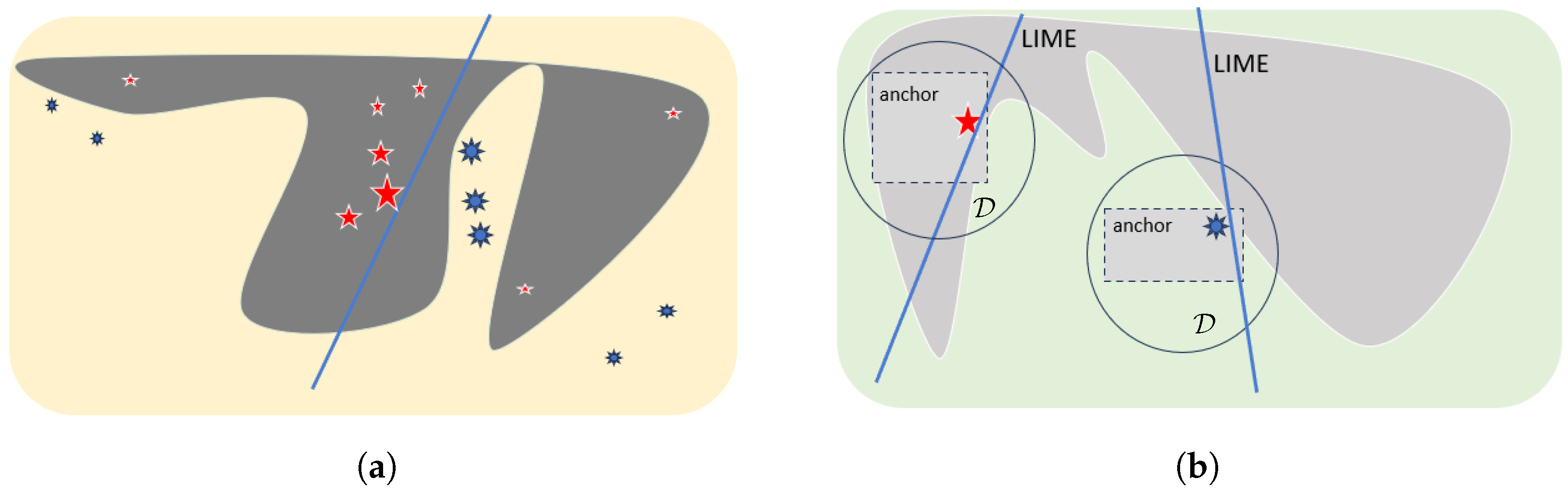
• if you are [younger than 50] and [female], then you are very unlikely to have cancer,
  where [age: under 50] and [gender: female] are referred to as anchors. As long as these anchors are present in new input, it is highly likely to be predicted as belonging to the same class as samples sharing these feature values. These features are assumed to cause the classification and provided that they are held; changes in the rest of the features do not affect the prediction. Similarly, for an image classification task, the anchors may be the following:
• if the given image includes [stripes], then it is almost guaranteed that the model will classify it correctly as a zebra,
  and hence the super-pixels involving [stripes] are called anchors. Anchors aim to meet two main requirements: precision and coverage. The former is about how precise the explanations are, while the latter defines the local area where these explanations are applicable. For a zebra classification task, precision is the percentage of perturbed examples from the same class as the input image that also contains [stripes], whereas coverage is defined as the fraction of the number of samples that hold the given anchor [stripes] to all perturbed instances [78].

Shapley Additive Explanations (SHAP) by Lundberg et al. is another powerful and widely used model-agnostic XAI approach [40]. It is rooted in the concept of Shapley values from cooperative game theory, where the goal is to fairly attribute the contribution to each player in a game based on their impact on the overall outcome. Applied to ML, SHAP assigns a value to each feature, representing its contribution to the final prediction for an individual instance. What makes SHAP particularly appealing is its theoretical rigour and its ability to provide consistent, model-agnostic explanations, making it highly versatile across different types of ML models, from linear to deep learning architectures. This versatility is achieved through several specialised variants designed to enhance both efficiency and accuracy depending on the model type. For instance, Kernel SHAP is the most general version, allowing SHAP values to be computed for any ML model. However, it relies on a kernel-based approximation technique that samples many combinations of feature subsets, which can be computationally intensive, particularly for high-dimensional data. Despite its flexibility, Kernel SHAP’s high computational cost often limits its scalability, especially for large datasets or complex models.

To address these performance limitations, model-specific variants of SHAP have been developed, with Tree SHAP [96] standing out as a prominent example. Tailored for tree-based models like decision trees, random forests, and gradient boosting machines, Tree SHAP leverages the structure of these models to compute exact SHAP values much more efficiently than Kernel SHAP. This makes it an ideal choice for structured data, where tree-based models are often preferred due to their predictive power and interpretability. In a similar vein, Deep SHAP combines SHAP values with DeepLIFT [88] to provide efficient explanations for deep learning models. By utilising backpropagation, Deep SHAP makes it feasible to explain complex neural networks in a computationally efficient manner, which is critical for tasks involving unstructured data like images or text.

These various SHAP variants highlight the method’s remarkable adaptability across different ML models which helped SHAP to become one of the cornerstone techniques in XAI. Its versatility in offering both local explanations (detailing the contributions of individual features to specific predictions) and broader global insights (captured through aggregations across the entire model) makes it an invaluable tool for diagnosing model behaviour, ensuring fairness, and promoting accountability in ML systems.

Perturbation-based XAI methodologies, such as SHAP and LIME, have gained considerable traction for their flexibility and ability to provide model-agnostic explanations. These methods excel at generating intuitive local explanations by estimating the contribution of individual features to a model’s predictions, making them valuable tools for interpreting complex ML models. Their general applicability across different model types is a significant strength, allowing practitioners to apply them to a wide range of tasks without requiring specific model architecture knowledge.

However, these methodologies are not without limitations. One significant challenge is their computational complexity. Estimating feature attributions often requires multiple model evaluations for various perturbed inputs, which can become infeasible for high-dimensional datasets or computationally expensive models. Another drawback is their reliance on assumptions about the data, such as feature independence, which is rarely true in real-world datasets. This can lead to misleading or less accurate interpretations in the presence of feature correlations. Additionally, while perturbation-based methods are effective at providing local explanations, deriving consistent global insights can be difficult, especially when local attributions vary widely across instances. Finally, being model-agnostic, these approaches might not fully capture the internal mechanics or nuances of a model, potentially limiting their utility in domains requiring a deep understanding of a model’s workings.

5. Conceptual Explanations

While visual explanations by activation maximisation and pixel attribution techniques are widely employed for computer vision tasks, there is also a growing interest in conceptual forms of explanations. Methodologies proposed in this direction aim to provide a high-level understanding of how models make decisions by linking their internal representations to human-interpretable concepts. This is particularly useful when the goal is to explain complex models in terms of concepts or features that align with human reasoning.

Network dissection [79] is a systematic methodology for interpreting the internal representations of neural networks by quantifying how individual neurons encode specific human-interpretable concepts. It provides a way to analyse the emergent structure within deep networks, particularly CNNs. The technique involves mapping the activation patterns of neurons to a predefined set of semantic concepts derived from labelled datasets, such as object categories, textures, or scenes. By evaluating the alignment between neuron activations and these concepts, network dissection enables researchers to understand the role and specialisation of neurons in the decision-making process of a model. This method is significant in demystifying the “black-box” nature of neural networks, providing insights into their transparency and interpretability, which are critical for debugging, enhancing trustworthiness, and identifying biases in AI systems.

Despite these advantages, network dissection has significant limitations. A key drawback is its reliance on segmentation maps for concepts, which are costly and time-consuming to create, especially for large and diverse datasets. This dependence can introduce biases and restrict the scope of analysis to predefined, segmented concepts, potentially overlooking emergent or complex features not present in the available segmentation maps. Additionally, network dissection focuses on individual units, which may fail to account for the collective behaviour of multiple units crucial for encoding higher-level abstractions. Lastly, it is better suited for static, pre-trained models and may struggle to offer insights for fine-tuned or dynamically evolving architectures.

Concept whitening [65] is another well-known technique. It works by modifying the latent space of neural networks to improve interpretability and disentanglement of learned representations. It introduces a specialised transformation layer into the network, which ensures that specific latent dimensions are decorrelated and aligned with human-understandable concepts. This is achieved through a whitening process that removes redundancy among features, making each dimension orthogonal to others while simultaneously associating them with predefined semantic concepts. By explicitly controlling the latent dimensions to represent interpretable concepts, concept whitening facilitates understanding and debugging of model behaviour and can potentially lead to better generalisation by reducing overfitting to irrelevant correlations in the data.

Concept activation vectors (CAVs), presented by Kim et al., represent one of the key methodologies in the concept-based explanations realm [66]. By defining a set of high-level concepts, such as “striped” or “spotted” for, say, animal classification, CAVs measure the alignment of these concepts with the model’s internal representations and allow researchers to examine how a deep learning model responds to these human-interpretable concepts. This is achieved by calculating directional derivatives of model predictions with respect to the predefined concepts at an intermediate layer of the examined model. This enables the generation of more meaningful explanations in the form of human-understandable concepts compared to the CNNs’ learnt high-level features or highlighted coarse-grained object locations. CAVs have been particularly valuable in medical imaging where model domain-specific explanations are crucial [97,98].

Crabbe et al. [99] proposed concept activation regions (CARs) which extend the CAV approach to address its limitations in modelling scattered concept examples in a DNN’s latent space. Unlike CAVs, which assume that concept examples align with a single direction in the latent space, CARs represent concepts as regions encompassing multiple clusters. This representation uses the kernel trick and support vector classifiers to define CARs. CARs enable describing how concepts relate to DNN predictions and also show how specific features correspond to concepts. Additionally, CARs demonstrate the potential for DNNs to autonomously identify established scientific concepts such as grading systems in prostate cancer analysis.

Presented as an extension to the earlier idea [100,101] of first predicting the concepts and then using the predicted concepts to predict a final target, concept bottleneck models (CBMs) [67] offer a compelling approach within the realm of conceptual explanations in XAI. These models were designed to provide interpretable decisions by incorporating human-understandable concepts into their decision-making process. In a CBM, the model first predicts a set of predefined concepts—such as “texture”, “shape”, or “tumour size”—which serve as high-level, interpretable features. These predicted concepts are then used as inputs to make the final decision. By doing so, CBMs allow users to directly inspect the model’s reasoning at an intermediate level, offering transparency into how each concept contributes to the outcome. This structured approach not only makes the decision-making process more understandable but also allows for interventions at the concept level, enabling users to correct mispredicted concepts before they affect the final output. In this direction, there have been several works exploring efficient ways to achieve systematic interventions and model corrections [102,103,104,105].

CBMs differ from CAVs in how they treat concepts. While CBMs are trained with the explicit goal of predicting and utilising predefined concepts as an integral part of their decision pipeline, CAVs operate in a post hoc manner. CAVs are used to probe and analyse a trained model’s internal representations to measure how well these representations align with specific concepts, without requiring the model to explicitly predict those concepts during training. In other words, CAVs extract and quantify the influence of concepts after the model has been trained, while CBMs actively incorporate and rely on concepts throughout the learning process. This distinction gives CBMs a unique advantage when it comes to interpretability and control, as they offer built-in transparency and allow for direct correction at the concept level, enhancing both the interpretability and robustness of the model. Several extensions were introduced to improve CBMs [106,107,108,109,110].

One key drawback of CBMs is their high cost as they require manual concept annotation for every training image. This process can be time-consuming and resource-intensive, especially when working with large datasets. One solution is proposed in [75] where class-wise attributes are used to train CBMs which significantly reduced the annotation cost. Another solution is to integrate CAVs [66] in CBMs, which requires only a set of positive and negative examples per concept, making them less annotation-intensive compared to the full concept annotations required by CBMs. Moreover, CAVs can even be derived from a completely different dataset to form concept banks which then can be employed to explain models trained with related datasets, making CAVs more flexible and scalable.

In this context, post hoc CBMs [69] achieve this integration to create a more efficient and controlled approach. They work by leveraging CAVs to obtain concept values, eliminating the need for intermediate concept predictions. Following that, a single layer is introduced as a bottleneck inspired by CBMs to map the concept values to the final classes. By doing so, post hoc CBMs maintain the model intervention property of traditional CBMs while avoiding the high costs of concept annotation for every image thanks to CAVs. This approach efficiently brings together the flexibility of CAVs and the structured decision-making process of CBMs, allowing for more scalable and transparent model analysis. Even though post hoc CBMs were shown to be effective as a global explicator via model editing experiments, their concept prediction and localisation abilities are under-explored. This is due to post hoc CBMs not being trained to explicitly predict the concepts unlike traditional CBMs, which hinders the possibility to do any direct evaluation on individual concept predictions.

Another methodology that aims to reduce the concept annotation cost, the CounTEX framework, connects image classifiers with textual concepts, leveraging a multi-modal embedding space, such as that provided by CLIP [111], to generate counterfactual explanations. It aims to explain classifier decisions by identifying and quantifying the contribution of specific, human-interpretable concepts derived from text. By mapping between the latent spaces of the target classifier and the CLIP model, CounTEX creates a projection mechanism to explain both correct and incorrect classifications in terms of these textual concepts. This approach aims to address the challenge of concept-annotated datasets requirement by utilising text-driven concepts [112].

An essential aspect of concept-based interpretability is the accurate prediction and localisation of highly important concepts. For example, if an animal classifier identifies an image as an antelope and indicates the horn as a critical concept for this prediction, the horn should not only be present in the input image but also activate the network in a way that aligns with the image region containing the horn.

While several methodologies discussed earlier provide relatively efficient solutions for concept-based explanations, their outputs are typically limited to a single level of abstraction. This means they lack the visual components necessary to highlight the precise regions corresponding to concepts in a given image. Furthermore, there is a noticeable absence of standardised evaluation metrics and benchmark datasets, making it challenging to compare these methodologies and comprehensively assess their strengths and limitations.

These gaps in concept-based explanation methodologies are addressed in [75], where the authors introduced their novel approach, Multilevel XAI, that generates both concepts and their corresponding heatmaps within the input image. Additionally, to address the lack of evaluation tools, Aysel et al. [113] proposed novel metrics for concept prediction and localisation while advocating for the use of an existing dataset, Caltech-UCSD Birds (CUB) [114], as a benchmark to evaluate concept-based explanation methodologies. These contributions enable more robust comparisons and comprehensive assessments of concept-based XAI methodologies.

6. XAI and Weakly Supervised Semantic Segmentation

Semantic segmentation is a core task in computer vision, focused on assigning semantically meaningful labels to every pixel in an image to identify specific objects. This task has diverse applications, including autonomous driving [115,116], scene understanding [117], and medical image analysis [118,119]. By enabling machines to extract detailed semantic information from images, it brings them closer to human-like visual perception. However, the inherent complexity and variability of real-world scenes, combined with the substantial need for labelled data to train deep learning models, make semantic segmentation a challenging problem. To tackle these difficulties, researchers have proposed various methods, such as fully convolutional networks (FCNs) [120], encoder–decoder architectures [121,122], and attention mechanisms [123]. These approaches have driven significant progress in semantic segmentation, establishing it as a vibrant and rapidly evolving research field.

Despite these architectural advancements, the requirement of pixel-wise segmentation maps remains a significant challenge for successful semantic segmentation applications. WSSS (weakly supervised semantic segmentation) approaches have been proposed to address this expensive per-pixel annotation challenge by leveraging less detailed coarse annotations, such as image-level labels, bounding boxes, scribbles, or points, to significantly reduce annotation efforts. Depending on the granularity and type of available annotations, weak supervision can be categorised into these types, each offering unique advantages and challenges that influence the methods and performance of WSSS approaches.

XAI has also emerged as a promising avenue for providing weak supervision in this context, offering significant potential for reducing reliance on fully annotated data. Techniques like Grad-CAM [80], LRP [68], and Integrated Gradients [74] generate saliency maps that highlight key regions contributing to a model’s predictions, making them valuable for WSSS. These outputs can serve as pseudo-annotations, guiding segmentation models by localising salient object parts. Hybrid approaches that combine XAI-generated pseudo-labels with weak annotations, such as image-level labels or bounding boxes, further enhance segmentation accuracy while minimising annotation costs. By aligning model interpretability with segmentation tasks, XAI fosters more transparent and explainable WSSS pipelines, bridging the gap between coarse annotations and precise segmentation, and ultimately reducing the need for dense supervision.

Below, we explore methodologies that utilise various levels of annotations, ranging from image-level labels to saliency maps generated by XAI techniques, as forms of weak supervision for semantic segmentation tasks. These methodologies were shown to be effective in outputting segmentation maps while keeping the annotation cost relatively low.

Image-level labels indicate the presence of classes in an image without providing spatial information. They are the weakest form of supervision as they lack localisation details. Methods using image-level labels often begin with CAM to localise discriminative regions associated with each class. While CAM-based approaches are computationally efficient, they tend to focus on the most salient parts of an object, leading to incomplete segmentations. Recent advancements aim to overcome these limitations through seed refinement, self-training, and affinity propagation, enabling broader and more accurate object coverage [124,125,126].

Bounding box annotations provide a coarse spatial indication of object locations, offering a balance between annotation cost and localisation precision. Early methods like BoxSup [127] refine segmentations iteratively within the boundaries defined by the boxes. Contemporary approaches integrate box constraints into deep learning models, achieving better spatial precision by aligning predicted masks with bounding box edges and leveraging region-based loss functions [128,129].

Scribbles and points serve as sparse spatial supervision, offering minimal yet explicit guidance about object locations. Scribble-based methods propagate annotations to unmarked regions using edge detection, graph-based propagation, or energy minimisation techniques [130,131,132]. Point-based methods rely on a few annotated pixels per object, often integrating these with background priors and unsupervised techniques to complete the segmentation [133].

A more recent methodology that gained attention is semantic proportion-based semantic segmentation (SPSS) [134], where only semantic proportions are utilised for semantic segmentation. Despite being several orders of magnitude cheaper than pixel-wise annotation in terms of annotation cost from both time and computational perspectives, SPSS is shown to be a promising WSSS methodology in several fields such as medical and aerial imaging, where obtaining full pixel annotation is challenging.

Several studies have demonstrated the use of XAI outputs as weak supervision for semantic segmentation, effectively bridging the gap between limited annotations and high-quality segmentation models [135,136]. For instance, HiResCAM-generated heatmaps have been used to refine annotations, enhancing segmentation models by highlighting relevant regions, particularly in complex image scenarios [137]. These approaches have been especially impactful in fields like medical imaging, where XAI-driven heatmaps help identify regions of interest for weakly supervised segmentation, reducing reliance on dense pixel-level annotations while improving model accuracy [138]. This integration of interpretability and weak supervision demonstrates the dual benefit of enhanced transparency and reduced annotation efforts.

Core approaches in WSSS revolve around generating and refining pseudo-labels, designing robust loss functions, and leveraging auxiliary information to improve segmentation accuracy. Loss functions are tailored to handle weak supervision, employing strategies to encourage confident predictions, and consistency regularisation to ensure stability under perturbations. Additionally, auxiliary cues, like saliency maps and edge detectors, help strengthen spatial information and guide model training.

The evaluation of WSSS methods relies on benchmark datasets and performance metrics that capture segmentation quality. Popular datasets, such as PASCAL VOC [139], MS COCO [140], and Cityscapes [141], provide a range of challenges in terms of object diversity, scale, and complexity. These datasets often include subsets tailored for weak supervision, with annotations like image-level labels or bounding boxes. The primary metric for assessing WSSS methods is Intersection over Union (IoU), which quantifies the overlap between predicted and ground-truth masks. To complement IoU, metrics like boundary accuracy and object localisation precision are sometimes used to provide finer insights into model performance. As WSSS research advances, the development of more diverse datasets and evaluation criteria will play a crucial role in driving progress and ensuring the robustness of these methods in real-world scenarios.

WSSS has emerged as a promising approach to address the high annotation costs associated with fully supervised methods, providing high-quality segmentation with minimal supervision. By utilising diverse forms of weak annotations, WSSS effectively balances annotation efficiency with segmentation performance. However, it still faces significant challenges such as localisation bias, where methods like CAM focus on the most discriminative object parts while neglecting less salient regions and noise in pseudo-labels, which can propagate errors during training. Scalability and generalisation also remain critical concerns, as models often struggle to adapt to diverse datasets and real-world scenarios. To address these challenges, recent trends include the adoption of transformer-based architectures [38] for capturing global and contextual information, contrastive learning to enhance pixel-level discrimination and robust strategies for mitigating pseudo-label noise. Additionally, hybrid supervision strategies, combining multiple weak annotations and domain adaptation techniques are gaining traction to improve generalisation across varied domains. As research continues to evolve, these advancements position WSSS as a key enabler for robust and scalable segmentation solutions across diverse applications.

7. Conclusions

As ML systems continue to integrate into high-stakes and decision-critical domains, the demand for transparency and interpretability has never been more urgent. This review presented a comprehensive examination of XAI methodologies, covering both post hoc and ad hoc approaches. We explored techniques ranging from low-level pixel-based saliency maps to high-level concept-based explanations, highlighting their respective advantages, limitations, and suitability across various application domains. While significant progress has been made in developing tools that help demystify black-box models, many challenges remain. Current methods often struggle to balance fidelity, human interpretability, and computational efficiency. Moreover, there is no universal standard for evaluating explanation quality, making it difficult to benchmark and compare approaches meaningfully. The relationship between XAI and weakly supervised learning, particularly in semantic segmentation, presents an exciting intersection where limited supervision automatically extracted by XAI methodology can be a good starting point. Looking forward, the field will benefit from more unified frameworks that integrate explanation into the learning process itself, as well as deeper collaboration between technical development and domain expertise. As trust in AI systems becomes increasingly intertwined with their explainability, the role of XAI will only become more central to responsible and reliable AI deployment.

References

1. Kim, C.; Gadgil, S.U.; DeGrave, A.J.; Omiye, J.A.; Cai, Z.R.; Daneshjou, R.; Lee, S.I. Transparent medical image AI via an image–text foundation model grounded in medical literature. Nat. Med. 2024, 30, 1154–1165. [Google Scholar] [CrossRef]
2. Wang, F.; Casalino, L.P.; Khullar, D. Deep learning in medicine—Promise, progress, and challenges. JAMA Intern. Med. 2019, 179, 293–294. [Google Scholar] [CrossRef]
3. Bogue, R. The role of artificial intelligence in robotics. Ind. Robot. Int. J. 2014, 41, 119–123. [Google Scholar] [CrossRef]
4. Soori, M.; Arezoo, B.; Dastres, R. Artificial intelligence, machine learning and deep learning in advanced robotics, a review. Cogn. Robot. 2023, 3, 54–70. [Google Scholar] [CrossRef]
5. Bickley, S.J.; Chan, H.F.; Torgler, B. Artificial intelligence in the field of economics. Scientometrics 2022, 127, 2055–2084. [Google Scholar] [CrossRef]
6. Redmon, J.; Divvala, S.; Girshick, R.; Farhadi, A. You only look once: Unified, real-time object detection. In Proceedings of the IEEE Conference on Computer Vision and Pattern Recognition, Las Vegas, NV, USA, 27–30 June 2016; pp. 779–788. [Google Scholar]
7. Kaur, R.; Singh, S. A comprehensive review of object detection with deep learning. Digit. Signal Process. 2023, 132, 103812. [Google Scholar] [CrossRef]
8. Akita, R.; Yoshihara, A.; Matsubara, T.; Uehara, K. Deep learning for stock prediction using numerical and textual information. In Proceedings of the 2016 IEEE/ACIS 15th International Conference on Computer and Information Science (ICIS), Okayama, Japan, 26–29 June 2016; IEEE: New York, NY, USA, 2016; pp. 1–6. [Google Scholar]
9. Ramesh, A.; Pavlov, M.; Goh, G.; Gray, S.; Voss, C.; Radford, A.; Chen, M.; Sutskever, I. Zero-shot text-to-image generation. In Proceedings of the International Conference on Machine Learning, PMLR, Virtual, 12–18 July 2021; pp. 8821–8831. [Google Scholar]
10. Xue, Z.; Song, G.; Guo, Q.; Liu, B.; Zong, Z.; Liu, Y.; Luo, P. Raphael: Text-to-image generation via large mixture of diffusion paths. Adv. Neural Inf. Process. Syst. 2024, 36. [Google Scholar] [CrossRef]
11. Singh, S.P.; Kumar, A.; Darbari, H.; Singh, L.; Rastogi, A.; Jain, S. Machine translation using deep learning: An overview. In Proceedings of the 2017 International Conference on Computer, Communications and Electronics (Comptelix), Jaipur, India, 1–2 July 2017; IEEE: New York, NY, USA, 2017; pp. 162–167. [Google Scholar]
12. Popel, M.; Tomkova, M.; Tomek, J.; Kaiser, Ł.; Uszkoreit, J.; Bojar, O.; Žabokrtskỳ, Z. Transforming machine translation: A deep learning system reaches news translation quality comparable to human professionals. Nat. Commun. 2020, 11, 4381. [Google Scholar] [CrossRef]
13. LeCun, Y.; Bengio, Y.; Hinton, G. Deep learning. Nature 2015, 521, 436–444. [Google Scholar] [CrossRef]
14. Deng, J.; Dong, W.; Socher, R.; Li, L.J.; Li, K.; Li, F.-F. Imagenet: A large-scale hierarchical image database. In Proceedings of the 2009 IEEE Conference on Computer Vision and Pattern Recognition, Miami, FL, USA, 20–25 June 2009; IEEE: New York, NY, USA, 2009; pp. 248–255. [Google Scholar]
15. Lindholm, E.; Nickolls, J.; Oberman, S.; Montrym, J. NVIDIA Tesla: A unified graphics and computing architecture. IEEE Micro 2008, 28, 39–55. [Google Scholar] [CrossRef]
16. Hassija, V.; Chamola, V.; Mahapatra, A.; Singal, A.; Goel, D.; Huang, K.; Scardapane, S.; Spinelli, I.; Mahmud, M.; Hussain, A. Interpreting black-box models: A review on explainable artificial intelligence. Cogn. Comput. 2024, 16, 45–74. [Google Scholar] [CrossRef]
17. Guidotti, R.; Monreale, A.; Ruggieri, S.; Turini, F.; Giannotti, F.; Pedreschi, D. A survey of methods for explaining black box models. ACM Comput. Surv. (CSUR) 2018, 51, 1–42. [Google Scholar] [CrossRef]
18. Ali, S.; Abuhmed, T.; El-Sappagh, S.; Muhammad, K.; Alonso-Moral, J.M.; Confalonieri, R.; Guidotti, R.; Del Ser, J.; Díaz-Rodríguez, N.; Herrera, F. Explainable Artificial Intelligence (XAI): What we know and what is left to attain Trustworthy Artificial Intelligence. Inf. Fusion 2023, 99, 101805. [Google Scholar] [CrossRef]
19. Hagras, H. Toward human-understandable, explainable AI. Computer 2018, 51, 28–36. [Google Scholar] [CrossRef]
20. Linardatos, P.; Papastefanopoulos, V.; Kotsiantis, S. Explainable ai: A review of machine learning interpretability methods. Entropy 2021, 23, 18. [Google Scholar] [CrossRef]
21. Gunning, D.; Aha, D. DARPA’s explainable artificial intelligence (XAI) program. AI Mag. 2019, 40, 44–58. [Google Scholar]
22. Doshi-Velez, F.; Kim, B. Towards a rigorous science of interpretable machine learning. arXiv 2017, arXiv:1702.08608. [Google Scholar]
23. Zhang, Y.; Tiňo, P.; Leonardis, A.; Tang, K. A survey on neural network interpretability. IEEE Trans. Emerg. Top. Comput. Intell. 2021, 5, 726–742. [Google Scholar] [CrossRef]
24. Lipton, Z.C. The mythos of model interpretability: In machine learning, the concept of interpretability is both important and slippery. Queue 2018, 16, 31–57. [Google Scholar] [CrossRef]
25. Arrieta, A.B.; Díaz-Rodríguez, N.; Del Ser, J.; Bennetot, A.; Tabik, S.; Barbado, A.; García, S.; Gil-López, S.; Molina, D.; Benjamins, R.; et al. Explainable Artificial Intelligence (XAI): Concepts, taxonomies, opportunities and challenges toward responsible AI. Inf. Fusion 2020, 58, 82–115. [Google Scholar] [CrossRef]
26. Das, A.; Rad, P. Opportunities and challenges in explainable artificial intelligence (xai): A survey. arXiv 2020, arXiv:2006.11371. [Google Scholar]
27. Tjoa, E.; Guan, C. A survey on explainable artificial intelligence (xai): Toward medical xai. IEEE Trans. Neural Netw. Learn. Syst. 2020, 32, 4793–4813. [Google Scholar] [CrossRef]
28. Meske, C.; Bunde, E. Transparency and trust in human-AI-interaction: The role of model-agnostic explanations in computer vision-based decision support. In Proceedings of the Artificial Intelligence in HCI: First International Conference, AI-HCI 2020, Held as Part of the 22nd HCI International Conference, HCII 2020, Copenhagen, Denmark, 19–24 July 2020; Proceedings 22. Springer: Berlin/Heidelberg, Germany, 2020; pp. 54–69. [Google Scholar]
29. Lipton, Z.C. The doctor just won’t accept that! Interpretable ML symposium. In Proceedings of the 31st Conference on Neural Information Processing Systems (NIPS 2017), Long Beach, CA, USA, 4–9 December 2017. [Google Scholar]
30. Bonicalzi, S. A matter of justice. The opacity of algorithmic decision-making and the trade-off between uniformity and discretion in legal applications of artificial intelligence. Teor. Riv. Filos. 2022, 42, 131–147. [Google Scholar]
31. Gilpin, L.H.; Bau, D.; Yuan, B.Z.; Bajwa, A.; Specter, M.; Kagal, L. Explaining explanations: An overview of interpretability of machine learning. In Proceedings of the 2018 IEEE 5th International Conference on data science and advanced analytics (DSAA), Turin, Italy, 1–4 October 2018; IEEE: New York, NY, USA, 2018; pp. 80–89. [Google Scholar]
32. Council of European Union. 2018 Reform of EU Data Protection Rules. 2018. Available online: https://gdpr.eu/ (accessed on 21 October 2024).
33. Adadi, A.; Berrada, M. Peeking inside the black-box: A survey on explainable artificial intelligence (XAI). IEEE Access 2018, 6, 52138–52160. [Google Scholar] [CrossRef]
34. Schwalbe, G.; Finzel, B. A comprehensive taxonomy for explainable artificial intelligence: A systematic survey of surveys on methods and concepts. Data Min. Knowl. Discov. 2024, 38, 3043–3101. [Google Scholar] [CrossRef]
35. Ahmed, I.; Jeon, G.; Piccialli, F. From artificial intelligence to explainable artificial intelligence in industry 4.0: A survey on what, how, and where. IEEE Trans. Ind. Inform. 2022, 18, 5031–5042. [Google Scholar] [CrossRef]
36. Hochreiter, S.; Schmidhuber, J. Long short-term memory. Neural Comput. 1997, 9, 1735–1780. [Google Scholar] [CrossRef]
37. Cho, K.; Van Merriënboer, B.; Bahdanau, D.; Bengio, Y. On the properties of neural machine translation: Encoder-decoder approaches. arXiv 2014, arXiv:1409.1259. [Google Scholar]
38. Vaswani, A. Attention is all you need. Adv. Neural Inf. Process. Syst. 2017, 30, 6000–6010. [Google Scholar]
39. Bento, J.; Saleiro, P.; Cruz, A.F.; Figueiredo, M.A.; Bizarro, P. Timeshap: Explaining recurrent models through sequence perturbations. In Proceedings of the 27th ACM SIGKDD Conference on Knowledge Discovery & Data Mining, Virtual Event Singapore, 14–18 August 2021; pp. 2565–2573. [Google Scholar]
40. Lundberg, S.M.; Lee, S.I. A unified approach to interpreting model predictions. In Proceedings of the 31st International Conference on Neural Information Processing Systems, Long Beach, CA, USA, 4–9 December 2017; pp. 4768–4777. [Google Scholar]
41. Rumelhart, D.E.; Hinton, G.E.; Williams, R.J. Learning representations by back-propagating errors. Nature 1986, 323, 533–536. [Google Scholar] [CrossRef]
42. Choi, E.; Bahadori, M.T.; Sun, J.; Kulas, J.; Schuetz, A.; Stewart, W. Retain: An interpretable predictive model for healthcare using reverse time attention mechanism. Adv. Neural Inf. Process. Syst. 2016, 29, 3512–3520. [Google Scholar]
43. Lim, B.; Arık, S.Ö.; Loeff, N.; Pfister, T. Temporal fusion transformers for interpretable multi-horizon time series forecasting. Int. J. Forecast. 2021, 37, 1748–1764. [Google Scholar] [CrossRef]
44. LeCun, Y.; Bottou, L.; Bengio, Y.; Haffner, P. Gradient-based learning applied to document recognition. Proc. IEEE 1998, 86, 2278–2324. [Google Scholar] [CrossRef]
45. Krizhevsky, A.; Sutskever, I.; Hinton, G.E. Imagenet classification with deep convolutional neural networks. Adv. Neural Inf. Process. Syst. 2012, 25, 1097–1105. [Google Scholar] [CrossRef]
46. Simonyan, K.; Zisserman, A. Very deep convolutional networks for large-scale image recognition. arXiv 2014, arXiv:1409.1556. [Google Scholar]
47. Szegedy, C.; Liu, W.; Jia, Y.; Sermanet, P.; Reed, S.; Anguelov, D.; Erhan, D.; Vanhoucke, V.; Rabinovich, A. Going deeper with convolutions. In Proceedings of the IEEE Conference on Computer Vision and Pattern Recognition, Boston, MA, USA, 7–12 June 2015; pp. 1–9. [Google Scholar]
48. He, K.; Zhang, X.; Ren, S.; Sun, J. Deep residual learning for image recognition. In Proceedings of the IEEE Conference on Computer Vision and Pattern Recognition (CVPR), Las Vegas, NV, USA, 27–30 June 2016. [Google Scholar]
49. Huang, G.; Liu, Z.; Van Der Maaten, L.; Weinberger, K.Q. Densely connected convolutional networks. In Proceedings of the IEEE Conference on Computer Vision and Pattern Recognition, Honolulu, HI, USA, 21–26 July 2017; pp. 4700–4708. [Google Scholar]
50. Howard, A.G. Mobilenets: Efficient convolutional neural networks for mobile vision applications. arXiv 2017, arXiv:1704.04861. [Google Scholar]
51. Tan, S.; Caruana, R.; Hooker, G.; Lou, Y. Detecting bias in black-box models using transparent model distillation. arXiv 2017, arXiv:1710.06169. [Google Scholar]
52. Liu, Z.; Mao, H.; Wu, C.Y.; Feichtenhofer, C.; Darrell, T.; Xie, S. A convnet for the 2020s. In Proceedings of the IEEE/CVF Conference on Computer Vision and Pattern Recognition, New Orleans, LA, USA, 18–25 June 2022; pp. 11976–11986. [Google Scholar]
53. Woo, S.; Debnath, S.; Hu, R.; Chen, X.; Liu, Z.; Kweon, I.S.; Xie, S. Convnext v2: Co-designing and scaling convnets with masked autoencoders. In Proceedings of the IEEE/CVF Conference on Computer Vision and Pattern Recognition, Vancouver, BC, Canada, 17–24 June 2023; pp. 16133–16142. [Google Scholar]
54. Quinlan, J.R. Induction of decision trees. Mach. Learn. 1986, 1, 81–106. [Google Scholar] [CrossRef]
55. Cristianini, N.; Shawe-Taylor, J. An Introduction to Support Vector Machines and Other Kernel-Based Learning Methods; Cambridge University Press: Cambridge, UK, 2000. [Google Scholar]
56. Dalal, N.; Triggs, B. Histograms of oriented gradients for human detection. In Proceedings of the 2005 IEEE Computer Society Conference on Computer Vision and Pattern Recognition, San Diego, CA, USA, 20–25 June 2005; IEEE: New York, NY, USA, 2005; Volume 1, pp. 886–893. [Google Scholar]
57. Lowe, D.G. Object recognition from local scale-invariant features. In Proceedings of the Seventh IEEE International Conference on Computer Vision, Corfu, Greece, 20–25 September 1999; IEEE: New York, NY, USA, 1999; Volume 2, pp. 1150–1157. [Google Scholar]
58. Hedjazi, M.A.; Kourbane, I.; Genc, Y. On identifying leaves: A comparison of CNN with classical ML methods. In Proceedings of the 2017 25th Signal Processing and Communications Applications Conference (SIU), Antalya, Turkey, 15–18 May 2017; pp. 1–4. [Google Scholar] [CrossRef]
59. Molnar, C. Interpretable Machine Learning; 2019. Available online: https://christophm.github.io/interpretable-ml-book/ (accessed on 20 February 2025).
60. Zeiler, M.D.; Fergus, R. Visualizing and understanding convolutional networks. In Proceedings of the European Conference on Computer Vision, Zurich, Switzerland, 6–12 September 2014; Springer: Berlin/Heidelberg, Germany, 2014; pp. 818–833. [Google Scholar]
61. Olah, C.; Alexander Mordvintsev, L.S. Feature Visualization. 2017. Available online: https://distill.pub/2017/feature-visualization/ (accessed on 12 January 2025).
62. Zhou, B.; Khosla, A.; Lapedriza, A.; Oliva, A.; Torralba, A. Object detectors emerge from training CNNs for scene recognition. In Proceedings of the 3rd International Conference on Learning Representations, San Diego, CA, USA, 7–9 May 2015; pp. 7–9. [Google Scholar]
63. Simonyan, K.; Vedaldi, A.; Zisserman, A. Deep inside convolutional networks: Visualising image classification models and saliency maps. In Proceedings of the Workshop at International Conference on Learning Representations, Citeseer, Banff, AB, Canada, 14–16 April 2014. [Google Scholar]
64. Wang, H.; Wang, Z.; Du, M.; Yang, F.; Zhang, Z.; Ding, S.; Mardziel, P.; Hu, X. Score-CAM: Score-weighted visual explanations for convolutional neural networks. In Proceedings of the IEEE/CVF Conference on Computer Vision and Pattern Recognition Workshops, Virtual, 14–19 June 2020; pp. 24–25. [Google Scholar]
65. Chen, Z.; Bei, Y.; Rudin, C. Concept whitening for interpretable image recognition. Nat. Mach. Intell. 2020, 2, 772–782. [Google Scholar] [CrossRef]
66. Kim, B.; Wattenberg, M.; Gilmer, J.; Cai, C.; Wexler, J.; Viegas, F.; Sayres, R. Interpretability beyond feature attribution: Quantitative testing with concept activation vectors (tcav). In Proceedings of the International Conference on Machine Learning, PMLR, Stockholm, Sweden, 10–15 July 2018; pp. 2668–2677. [Google Scholar]
67. Koh, P.W.; Nguyen, T.; Tang, Y.S.; Mussmann, S.; Pierson, E.; Kim, B.; Liang, P. Concept bottleneck models. In Proceedings of the International Conference on Machine Learning, PMLR, Virtual, 13–18 July 2020; pp. 5338–5348. [Google Scholar]
68. Bach, S.; Binder, A.; Montavon, G.; Klauschen, F.; Müller, K.R.; Samek, W. On pixel-wise explanations for non-linear classifier decisions by layer-wise relevance propagation. PLoS ONE 2015, 10, e0130140. [Google Scholar] [CrossRef]
69. Yuksekgonul, M.; Wang, M.; Zou, J. Post-hoc concept bottleneck models. In Proceedings of the Eleventh International Conference on Learning Representations, Kigali, Rwanda, 1–5 May 2023. [Google Scholar]
70. Nguyen, A.; Yosinski, J.; Clune, J. Multifaceted feature visualization: Uncovering the different types of features learned by each neuron in deep neural networks. arXiv 2016, arXiv:1602.03616. [Google Scholar]
71. Borowski, J.; Zimmermann, R.S.; Schepers, J.; Geirhos, R.; Wallis, T.S.; Bethge, M.; Brendel, W. Exemplary natural images explain CNN activations better than state-of-the-art feature visualization. arXiv 2020, arXiv:2010.12606. [Google Scholar]
72. Cammarata, N.; Goh, G.; Carter, S.; Schubert, L.; Petrov, M.; Olah, C.; Curve Detectors. Distill 2020. Available online: https://distill.pub/2020/circuits/curve-detectors (accessed on 10 December 2024).
73. Springenberg, J.T.; Dosovitskiy, A.; Brox, T.; Riedmiller, M. Striving for simplicity: The all convolutional net. arXiv 2014, arXiv:1412.6806. [Google Scholar]
74. Sundararajan, M.; Taly, A.; Yan, Q. Axiomatic attribution for deep networks. In Proceedings of the International Conference on Machine Learning, PMLR, Sydney, Australia, 6–11 August 2017; pp. 3319–3328. [Google Scholar]
75. Aysel, H.I.; Cai, X.; Prugel-Bennett, A. Multilevel explainable artificial intelligence: Visual and linguistic bonded explanations. IEEE Trans. Artif. Intell. 2023, 5, 2055–2066. [Google Scholar] [CrossRef]
76. Zhou, B.; Khosla, A.; Lapedriza, A.; Oliva, A.; Torralba, A. Learning deep features for discriminative localization. In Proceedings of the IEEE Conference on Computer Vision and Pattern Recognition, Las Vegas, NV, USA, 27–30 June 2016; pp. 2921–2929. [Google Scholar]
77. Ribeiro, M.T.; Singh, S.; Guestrin, C. “Why should i trust you?” Explaining the predictions of any classifier. In Proceedings of the 22nd ACM SIGKDD International Conference on Knowledge Discovery and Data Mining, San Francisco, CA, USA, 13–17 August 2016; pp. 1135–1144. [Google Scholar]
78. Ribeiro, M.T.; Singh, S.; Guestrin, C. Anchors: High-precision model-agnostic explanations. In Proceedings of the AAAI Conference on Artificial Intelligence, New Orleans, LA, USA, 2–7 February 2018. [Google Scholar]
79. Bau, D.; Zhou, B.; Khosla, A.; Oliva, A.; Torralba, A. Network dissection: Quantifying interpretability of deep visual representations. In Proceedings of the IEEE Conference on Computer Vision and Pattern Recognition, Honolulu, HI, USA, 21–26 July 2017; pp. 6541–6549. [Google Scholar]
80. Selvaraju, R.R.; Cogswell, M.; Das, A.; Vedantam, R.; Parikh, D.; Batra, D. Grad-CAM: Visual explanations from deep networks via gradient-based localization. In Proceedings of the IEEE International Conference on Computer Vision (ICCV), Venice, Italy, 22–29 October 2017. [Google Scholar]
81. Muddamsetty, S.M.; Mohammad, N.J.; Moeslund, T.B. Sidu: Similarity difference and uniqueness method for explainable ai. In Proceedings of the 2020 IEEE International Conference on Image Processing (ICIP), Virtual, 25–28 October; IEEE: New York, NY, USA, 2020; pp. 3269–3273. [Google Scholar]
82. Petsiuk, V.; Das, A.; Saenko, K. Rise: Randomized input sampling for explanation of black-box models. arXiv 2018, arXiv:1806.07421. [Google Scholar]
83. Wexler, J.; Pushkarna, M.; Bolukbasi, T.; Wattenberg, M.; Viégas, F.; Wilson, J. The what-if tool: Interactive probing of machine learning models. IEEE Trans. Vis. Comput. Graph. 2019, 26, 56–65. [Google Scholar] [CrossRef]
84. Arya, V.; Bellamy, R.K.; Chen, P.Y.; Dhurandhar, A.; Hind, M.; Hoffman, S.C.; Houde, S.; Liao, Q.V.; Luss, R.; Mojsilović, A.; et al. Ai explainability 360 toolkit. In Proceedings of the 3rd ACM India Joint International Conference on Data Science & Management of Data (8th ACM IKDD CODS & 26th COMAD), Bangalore, India, 2–4 January 2021; pp. 376–379. [Google Scholar]
85. LeDell, E.; Poirier, S. H2O AutoML: Scalable automatic machine learning. In Proceedings of the AutoML Workshop at ICML, ICML, San Diego, CA, USA, Virtual, 12–18 July 2020; Volume 2020. [Google Scholar]
86. Yosinski, J.; Clune, J.; Nguyen, A.; Fuchs, T.; Lipson, H. Understanding neural networks through deep visualization. arXiv 2015, arXiv:1506.06579. [Google Scholar]
87. Zeiler, M.D.; Taylor, G.W.; Fergus, R. Adaptive deconvolutional networks for mid and high level feature learning. In Proceedings of the 2011 International Conference on Computer Vision, Barcelona, Spain, 6–13 November 2011; IEEE: New York, NY, USA, 2011; pp. 2018–2025. [Google Scholar]
88. Shrikumar, A.; Greenside, P.; Kundaje, A. Learning important features through propagating activation differences. In Proceedings of the International Conference on Machine Learning, PMlR, Sydney, Australia, 6–11 August 2017; pp. 3145–3153. [Google Scholar]
89. Kohlbrenner, M.; Bauer, A.; Nakajima, S.; Binder, A.; Samek, W.; Lapuschkin, S. Towards best practice in explaining neural network decisions with LRP. In Proceedings of the 2020 International Joint Conference on Neural Networks (IJCNN), Glasgow, UK, 19–24 July 2020; IEEE: New York, NY, USA, 2020; pp. 1–7. [Google Scholar]
90. Montavon, G.; Binder, A.; Lapuschkin, S.; Samek, W.; Müller, K.R. Layer-wise relevance propagation: An overview. In Explainable AI: Interpreting, Explaining and Visualizing Deep Learning; Springer: Berlin/Heidelberg, Germany, 2019; pp. 193–209. [Google Scholar]
91. Jung, Y.J.; Han, S.H.; Choi, H.J. Explaining CNN and RNN using selective layer-wise relevance propagation. IEEE Access 2021, 9, 18670–18681. [Google Scholar] [CrossRef]
92. Hollister, J.D.; Cai, X.; Horton, T.; Price, B.W.; Zarzyczny, K.M.; Fenberg, P.B. Using computer vision to identify limpets from their shells: A case study using four species from the Baja California peninsula. Front. Mar. Sci. 2023, 10, 1167818. [Google Scholar] [CrossRef]
93. Chattopadhay, A.; Sarkar, A.; Howlader, P.; Balasubramanian, V.N. Grad-cam++: Generalized gradient-based visual explanations for deep convolutional networks. In Proceedings of the 2018 IEEE Winter Conference on Applications of Computer Vision (WACV), Lake Tahoe, NV, USA, 12–15 March 2018; IEEE: New York, NY, USA, 2018; pp. 839–847. [Google Scholar]
94. Li, X.; Xiong, H.; Li, X.; Zhang, X.; Liu, J.; Jiang, H.; Chen, Z.; Dou, D. G-LIME: Statistical learning for local interpretations of deep neural networks using global priors. Artif. Intell. 2023, 314, 103823. [Google Scholar] [CrossRef]
95. Zhou, Z.; Hooker, G.; Wang, F. S-lime: Stabilized-lime for model explanation. In Proceedings of the 27th ACM SIGKDD Conference on Knowledge Discovery & Data Mining, Virtual, 14–18 August 2021; pp. 2429–2438. [Google Scholar]
96. Lundberg, S.M.; Erion, G.G.; Lee, S.I. Consistent individualized feature attribution for tree ensembles. arXiv 2018, arXiv:1802.03888. [Google Scholar]
97. Lucieri, A.; Bajwa, M.N.; Braun, S.A.; Malik, M.I.; Dengel, A.; Ahmed, S. On interpretability of deep learning based skin lesion classifiers using concept activation vectors. In Proceedings of the 2020 International Joint Conference on Neural Networks (IJCNN), Glasgow, UK, 19–24 July 2020; IEEE: New York, NY, USA, 2020; pp. 1–10. [Google Scholar]
98. Correa, R.; Pahwa, K.; Patel, B.; Vachon, C.M.; Gichoya, J.W.; Banerjee, I. Efficient adversarial debiasing with concept activation vector—Medical image case-studies. J. Biomed. Inform. 2024, 149, 104548. [Google Scholar] [CrossRef]
99. Crabbé, J.; van der Schaar, M. Concept activation regions: A generalized framework for concept-based explanations. Adv. Neural Inf. Process. Syst. 2022, 35, 2590–2607. [Google Scholar]
100. Kumar, N.; Berg, A.C.; Belhumeur, P.N.; Nayar, S.K. Attribute and simile classifiers for face verification. In Proceedings of the 2009 IEEE 12th International Conference on Computer Vision, Kyoto, Japan, 29 September–2 October 2009; IEEE: New York, NY, USA, 2009; pp. 365–372. [Google Scholar]
101. Lampert, C.H.; Nickisch, H.; Harmeling, S. Learning to detect unseen object classes by between-class attribute transfer. In Proceedings of the 2009 IEEE Conference on Computer Vision and Pattern Recognition, Miami, FL, USA, 20–25 June 2009; IEEE: New York, NY, USA, 2009; pp. 951–958. [Google Scholar]
102. Steinmann, D.; Stammer, W.; Friedrich, F.; Kersting, K. Learning to intervene on concept bottlenecks. In Proceedings of the 41st International Conference on Machine Learning, Vienna, Austria, 21–27 July 2024; Salakhutdinov, R., Kolter, Z., Heller, K., Weller, A., Oliver, N., Scarlett, J., Berkenkamp, F., Eds.; PMLR: Cambridge, MA, USA, 2024. Proceedings of Machine Learning Research. Volume 235, pp. 46556–46571. [Google Scholar]
103. Shin, S.; Jo, Y.; Ahn, S.; Lee, N. A closer look at the intervention procedure of concept bottleneck models. In Proceedings of the International Conference on Machine Learning, PMLR, Honolulu, HI, USA, 23–29 July 2023; pp. 31504–31520. [Google Scholar]
104. Singhi, N.; Kim, J.M.; Roth, K.; Akata, Z. Improving intervention efficacy via concept realignment in concept bottleneck models. In Proceedings of the European Conference on Computer Vision, Paris, France, 26–27 March 2025; Springer: Berlin/Heidelberg, Germany, 2025; pp. 422–438. [Google Scholar]
105. Chauhan, K.; Tiwari, R.; Freyberg, J.; Shenoy, P.; Dvijotham, K. Interactive concept bottleneck models. In Proceedings of the AAAI Conference on Artificial Intelligence, Washington, DC, USA, 7–14 February 2023; Volume 37, pp. 5948–5955. [Google Scholar]
106. Vandenhirtz, M.; Laguna, S.; Marcinkevičs, R.; Vogt, J.E. Stochastic concept bottleneck models. In Proceedings of the ICML 2024 Workshop on Structured Probabilistic Inference & Generative Modeling, Vienna, Austria, 21–27 July 2024. [Google Scholar]
107. Havasi, M.; Parbhoo, S.; Doshi-Velez, F. Addressing leakage in concept bottleneck models. In Proceedings of the Advances in Neural Information Processing Systems; Koyejo, S., Mohamed, S., Agarwal, A., Belgrave, D., Cho, K., Oh, A., Eds.; Curran Associates, Inc.: Red Hook, NY, USA, 2022; Volume 35, pp. 23386–23397. [Google Scholar]
108. Hu, L.; Ren, C.; Hu, Z.; Lin, H.; Wang, C.L.; Xiong, H.; Zhang, J.; Wang, D. Editable concept bottleneck models. arXiv 2024, arXiv:2405.15476. [Google Scholar]
109. Kim, E.; Jung, D.; Park, S.; Kim, S.; Yoon, S. Probabilistic concept bottleneck models. In Proceedings of the 40th International Conference on Machine Learning, JMLR.org, Honolulu, HI, USA, 23–29 July 2023. ICML’23. [Google Scholar]
110. Shang, C.; Zhou, S.; Zhang, H.; Ni, X.; Yang, Y.; Wang, Y. Incremental residual concept bottleneck models. In Proceedings of the IEEE/CVF Conference on Computer Vision and Pattern Recognition, Seattle, WA, USA, 16–2 June 2024; pp. 11030–11040. [Google Scholar]
111. Radford, A.; Kim, J.W.; Hallacy, C.; Ramesh, A.; Goh, G.; Agarwal, S.; Sastry, G.; Askell, A.; Mishkin, P.; Clark, J.; et al. Learning transferable visual models from natural language supervision. In Proceedings of the International Conference on Machine Learning, PMLR, Virtual, 18–24 July 2021; pp. 8748–8763. [Google Scholar]
112. Kim, S.; Oh, J.; Lee, S.; Yu, S.; Do, J.; Taghavi, T. Grounding counterfactual explanation of image classifiers to textual concept space. In Proceedings of the IEEE/CVF Conference on Computer Vision and Pattern Recognition, Vancouver, BC, Canada, 17–24 June 2023; pp. 10942–10950. [Google Scholar]
113. Aysel, H.I.; Cai, X.; Prugel-Bennett, A. Concept-based explainable artificial intelligence: Metrics and benchmarks. arXiv 2025, arXiv:2501.19271. [Google Scholar]
114. Wah, C.; Branson, S.; Welinder, P.; Perona, P.; Belongie, S. The Caltech-Ucsd Birds-200-2011 Dataset. 2011. Available online: https://www.vision.caltech.edu/datasets/cub_200_2011/ (accessed on 24 June 2025).
115. Feng, D.; Haase-Schütz, C.; Rosenbaum, L.; Hertlein, H.; Glaeser, C.; Timm, F.; Wiesbeck, W.; Dietmayer, K. Deep multi-modal object detection and semantic segmentation for autonomous driving: Datasets, methods, and challenges. IEEE Trans. Intell. Transp. Syst. 2020, 22, 1341–1360. [Google Scholar] [CrossRef]
116. Siam, M.; Gamal, M.; Abdel-Razek, M.; Yogamani, S.; Jagersand, M.; Zhang, H. A comparative study of real-time semantic segmentation for autonomous driving. In Proceedings of the IEEE Conference on Computer Vision and Pattern Recognition Workshops, Salt Lake City, UT, USA, 18–23 June 2018; pp. 587–597. [Google Scholar]
117. Chen, R.; Liu, Y.; Kong, L.; Zhu, X.; Ma, Y.; Li, Y.; Hou, Y.; Qiao, Y.; Wang, W. Clip2scene: Towards label-efficient 3d scene understanding by clip. In Proceedings of the IEEE/CVF Conference on Computer Vision and Pattern Recognition, Vancouver, BC, Canada, 17–24 June 2023; pp. 7020–7030. [Google Scholar]
118. Qureshi, I.; Yan, J.; Abbas, Q.; Shaheed, K.; Riaz, A.B.; Wahid, A.; Khan, M.W.J.; Szczuko, P. Medical image segmentation using deep semantic-based methods: A review of techniques, applications and emerging trends. Inf. Fusion 2023, 90, 316–352. [Google Scholar] [CrossRef]
119. Dhamija, T.; Gupta, A.; Gupta, S.; Anjum; Katarya, R.; Singh, G. Semantic segmentation in medical images through transfused convolution and transformer networks. Appl. Intell. 2023, 53, 1132–1148. [Google Scholar] [CrossRef]
120. Long, J.; Shelhamer, E.; Darrell, T. Fully convolutional networks for semantic segmentation. In Proceedings of the IEEE Conference on Computer Vision and Pattern Recognition, Boston, MA, USA, 7–12 June 2015; pp. 3431–3440. [Google Scholar]
121. Chen, L.C.; Papandreou, G.; Kokkinos, I.; Murphy, K.; Yuille, A.L. Deeplab: Semantic image segmentation with deep convolutional nets, atrous convolution, and fully connected CRFs. IEEE Trans. Pattern Anal. Mach. Intell. 2017, 40, 834–848. [Google Scholar] [CrossRef]
122. Chen, L.C.; Zhu, Y.; Papandreou, G.; Schroff, F.; Adam, H. Encoder-decoder with atrous separable convolution for semantic image segmentation. In Proceedings of the European Conference on Computer Vision (ECCV), Munich, Germany, 8–14 September 2018; pp. 801–818. [Google Scholar]
123. Zhong, Z.; Lin, Z.Q.; Bidart, R.; Hu, X.; Daya, I.B.; Li, Z.; Zheng, W.S.; Li, J.; Wong, A. Squeeze-and-attention networks for semantic segmentation. In Proceedings of the IEEE/CVF Conference on Computer Vision and Pattern Recognition, Seattle, WA, USA, 13–19 June 2020; pp. 13065–13074. [Google Scholar]
124. Chen, Z.; Sun, Q. Weakly-supervised semantic segmentation with image-level labels: From traditional models to foundation models. ACM Comput. Surv. 2023, 57, 111. [Google Scholar] [CrossRef]
125. Papandreou, G.; Chen, L.C.; Murphy, K.P.; Yuille, A.L. Weakly-and semi-supervised learning of a deep convolutional network for semantic image segmentation. In Proceedings of the IEEE International Conference on Computer Vision, Santiago, Chile, 7–13 December 2015; pp. 1742–1750. [Google Scholar]
126. Kolesnikov, A.; Lampert, C.H. Seed, expand and constrain: Three principles for weakly-supervised image segmentation. In Proceedings of the Computer Vision–ECCV, Amsterdam, The Netherlands, 11–14 October 2016; Springer: Berlin/Heidelberg, Germany, 2016; pp. 695–711. [Google Scholar]
127. Dai, J.; He, K.; Sun, J. Boxsup: Exploiting bounding boxes to supervise convolutional networks for semantic segmentation. In Proceedings of the IEEE International Conference on Computer Vision, Santiago, Chile, 7–13 December 2015; pp. 1635–1643. [Google Scholar]
128. Lee, J.; Yi, J.; Shin, C.; Yoon, S. Bbam: Bounding box attribution map for weakly supervised semantic and instance segmentation. In Proceedings of the IEEE/CVF Conference on Computer Vision and Pattern Recognition, Nashville, TN, USA, 20–25 June 2021; pp. 2643–2652. [Google Scholar]
129. Song, C.; Huang, Y.; Ouyang, W.; Wang, L. Box-driven class-wise region masking and filling rate guided loss for weakly supervised semantic segmentation. In Proceedings of the IEEE/CVF Conference on Computer Vision and Pattern Recognition, Long Beach, CA, USA, 15–20 June 2019; pp. 3136–3145. [Google Scholar]
130. Lin, D.; Dai, J.; Jia, J.; He, K.; Sun, J. Scribblesup: Scribble-supervised convolutional networks for semantic segmentation. In Proceedings of the IEEE Conference on Computer Vision and Pattern Recognition, Las Vegas, NV, USA, 27–30 June 2016; pp. 3159–3167. [Google Scholar]
131. Lee, H.; Jeong, W.K. Scribble2label: Scribble-supervised cell segmentation via self-generating pseudo-labels with consistency. In Proceedings of the Medical Image Computing and Computer Assisted Intervention–MICCAI 2020: 23rd International Conference, Lima, Peru, 4–8 October 2020; Proceedings, Part I 23. Springer: Berlin/Heidelberg, Germany, 2020; pp. 14–23. [Google Scholar]
132. Vernaza, P.; Chandraker, M. Learning random-walk label propagation for weakly-supervised semantic segmentation. In Proceedings of the IEEE Conference on Computer Vision and Pattern Recognition, Honolulu, HI, USA, 21–26 July 2017; pp. 7158–7166. [Google Scholar]
133. Bearman, A.; Russakovsky, O.; Ferrari, V.; Li, F.-F. What’s the point: Semantic segmentation with point supervision. In Proceedings of the European Conference on Computer Vision, Amsterdam, The Netherlands, 11–14 October 2016; Springer: Berlin/Heidelberg, Germany, 2016; pp. 549–565. [Google Scholar]
134. Aysel, H.I.; Cai, X.; Prügel-Bennett, A. Semantic segmentation by semantic proportions. arXiv 2023, arXiv:2305.15608. [Google Scholar]
135. Liu, Y.; Lian, L.; Zhang, E.; Xu, L.; Xiao, C.; Zhong, X.; Li, F.; Jiang, B.; Dong, Y.; Ma, L.; et al. Mixed-UNet: Refined class activation mapping for weakly-supervised semantic segmentation with multi-scale inference. Front. Comput. Sci. 2022, 4, 1036934. [Google Scholar] [CrossRef]
136. Seibold, C.; Künzel, J.; Hilsmann, A.; Eisert, P. From explanations to segmentation: Using explainable AI for image segmentation. arXiv 2022, arXiv:2202.00315. [Google Scholar]
137. Draelos, R.L.; Carin, L. Use HiResCAM instead of Grad-CAM for faithful explanations of convolutional neural networks. arXiv 2020, arXiv:2011.08891. [Google Scholar]
138. Gipiškis, R.; Tsai, C.W.; Kurasova, O. Explainable AI (XAI) in image segmentation in medicine, industry, and beyond: A survey. ICT Express 2024, 10, 1331–1354. [Google Scholar] [CrossRef]
139. Everingham, M.; Van Gool, L.; Williams, C.K.; Winn, J.; Zisserman, A. The Pascal Visual Object Classes (VOC) Challenge. Int. J. Comput. Vis. 2010, 88, 303–338. [Google Scholar] [CrossRef]
140. Lin, T.Y.; Maire, M.; Belongie, S.; Hays, J.; Perona, P.; Ramanan, D.; Dollár, P.; Zitnick, C.L. Microsoft coco: Common objects in context. In Proceedings of the Computer Vision–ECCV 2014: 13th European Conference, Zurich, Switzerland, 6–12 September 2014; Proceedings, Part V 13. Springer: Berlin/Heidelberg, Germany, 2014; pp. 740–755. [Google Scholar]
141. Cordts, M.; Omran, M.; Ramos, S.; Rehfeld, T.; Enzweiler, M.; Benenson, R.; Franke, U.; Roth, S.; Schiele, B. The cityscapes dataset for semantic urban scene understanding. In Proceedings of the IEEE Conference on Computer Vision and Pattern Recognition, Las Vegas, NV, USA, 27–30 June 2016; pp. 3213–3223. [Google Scholar]
Figure 1. XAI dimensions for various applications.
Applsci 15 07261 g001
Figure 2. An overview of XAI methodologies based on their modalities.
Applsci 15 07261 g002
Figure 3. An overview of GradCAM (gradient-weighted class activation mapping) [80]. Gradients of the predicted class score with respect to the feature maps of the last convolutional layer are computed to obtain weights w c . These weights are used to linearly combine the feature maps, and the resulting weighted sum is used to mask the input image to obtain a saliency map, highlighting the regions most relevant to the prediction.
Applsci 15 07261 g003
Figure 4. The difference between LIME (a) and Anchors approaches (b). LIME fits the best possible linear line while anchors “guarantee” that almost all the examples satisfying the rules are from the same class. D is the perturbation space for both approaches, the straight blue line is the linear model that LIME proposes, and the dashed box is the local area that the Anchor method “anchors” the explanations. (a) LIME. Adapted from [77]. (b) Anchors. Adapted from [78].
Applsci 15 07261 g004
Disclaimer/Publisher’s Note: The statements, opinions and data contained in all publications are solely those of the individual author(s) and contributor(s) and not of MDPI and/or the editor(s). MDPI and/or the editor(s) disclaim responsibility for any injury to people or property resulting from any ideas, methods, instructions or products referred to in the content.