A Comparative Study of Advanced Transformer Learning Frameworks for Water Potability Analysis Using Physicochemical Parameters

Abstract

Keeping drinking water safe is a critical aspect of protecting public health. Traditional laboratory-based methods for evaluating water potability are often time-consuming, costly, and labour-intensive. This paper presents a comparative analysis of four transformer-based deep learning models in the development of automatic classification systems for water potability based on physicochemical attributes. The models examined include the enhanced tabular transformer (ETT), feature tokenizer transformer (FTTransformer), self-attention and inter-sample network (SAINT), and tabular autoencoder pretraining enhancement (TAPE). The study utilized an open-access water quality dataset that includes nine key attributes such as pH, hardness, total dissolved solids (TDS), chloramines, sulphate, conductivity, organic carbon, trihalomethanes, and turbidity. The models were evaluated under a unified protocol involving 70–15–15 data partitioning, five-fold cross-validation, fixed random seed, and consistent hyperparameter settings. Among the evaluated models, the enhanced tabular transformer outperforms other models with an accuracy of 95.04% and an F1 score of 0.94. ETT is an advanced model because it can efficiently model high-order feature interactions through multi-head attention and deep hierarchical encoding. Feature importance analysis consistently highlighted chloramines, conductivity, and trihalomethanes as key predictive features across all models. SAINT demonstrated robust generalization through its dual-attention mechanism, while TAPE provided competitive results with reduced computational overhead due to unsupervised pretraining. Conversely, FTTransformer showed limitations, likely due to sensitivity to class imbalance and hyperparameter tuning. The results underscore the potential of transformer-based models, especially ETT, in enabling efficient, accurate, and scalable water quality monitoring. These findings support their integration into real-time environmental health systems and suggest approaches for future research in explainability, domain adaptation, and multimodal fusion.

1. Introduction

The provision of safe drinking water is not only an essential global health priority but also a major component of Sustainable Development Goal 6 of the United Nations. Although awareness of safe drinking water increased globally, many people still rely on unsafe water sources for consumption and daily use. As of 2022, it is estimated that approximately 1.7 billion people are using drinking water contaminated with feces, leading to horrible health consequences. Consumption of microbially contaminated water can lead to waterborne diseases such as diarrhea, cholera, typhoid, and hepatitis A. These diseases cause a huge number of deaths in the low-income world, with hundreds of preventable deaths each year [1]. The impact of this disease is especially high for children under five years of age. Thus, the availability of safe drinking water and its sustainable management are not only a public health need, but also a matter of social and economic concern.

It is vital for preventing disease outbreaks and ensuring human health that the water quality parameters are tracked continuously and accurately. Traditional methods for water quality assessment include periodic laboratory analyses of physicochemical and microbiological parameters, which are time-consuming, labor-intensive, and costly. Complementarily, there has been a growing interest in computational prediction methods based on measurable water quality indicators. Machine learning (ML) techniques are potentially good candidates for classifying water potability automatically based on sensor data. Classical algorithms, such as decision trees, support vector machines (SVMs), k-nearest neighbors (KNN), and ensemble algorithms (random forest, AdaBoost, and XGBoost), have found great applications in this context. Among these, XGBoost emerged as a preferred method for handling large and heterogeneous datasets due to its capacity to manage missing values and model complex feature interactions. Empirical studies have shown that such tree-based models consistently outperform simpler classifiers such as logistic regression [2,3]. Nonetheless, conventional ML models often depend on manual feature engineering and may fail to capture the subtle nonlinear dependencies among water quality attributes. The above limitations are addressed by proposing deep learning as an alternative. It is a data-driven approach, where feature representations are learned automatically in an abstract manner. Nevertheless, it has been a point of contention as to whether classical multilayer perceptron’s (MLPs) can outperform ensemble techniques on tabular datasets [4]. Thus, attempts to bridge this uncomfortable distance led to the conception of specialized neural architectures accommodating structured data. One of the most promising research directions in this context has been the exploration of attention mechanisms. For example, TabNet does sequential attention-based feature selection wherein the dynamic assignment of importance is given to the relevant features developed from each decision step to achieve high accuracy with interpretability [5]. Correspondingly, the TabTransformer adopts the self-attention approach characteristic of transformers to encode categorical variables for tabular data, which exhibited a performance level commensurate with state-of-the-art ensemble methods [6].

More recent transformer-based architectures, such as FTTransformer, embed each feature as a token and apply multi-head self-attention to model inter-feature relationships, thereby achieving or surpassing other deep learning approaches on structured prediction tasks [4]. SAINT extends this capability by introducing a dual-attention mechanism that models both feature-wise and row-wise dependencies. Moreover, with appropriate contrastive self-supervised pretraining, SAINT performed much better than the widely used ensemble methods XGBoost and LightGBM across different benchmarks [7]. Unsupervised techniques using deep autoencoder-based models are designed to learn compressed representations in suitably unlabeled time series data for performing anomaly detection under real-world low-label conditions. For instance, Amarbayasgalan et al. [8] proposed an unsupervised anomaly detection method based on reconstruction error that has shown increased performance across 52 benchmark datasets over different domains. These methods are extremely attractive in the environmental sciences, considering the scarcity of annotated data that is quite expensive to acquire.

In spite of deep tabular learning’s advancement, its role in water quality classification, especially drinking water potability, remains a less explored area. Most of the literature concentrated on conventional ML methods. Very few studies involve comparative analyses of contemporary attention-based deep learning architectures within this area. For these reasons, this study aims to present the following objectives to fill this gap and further drive the current body of knowledge:

• Comparative evaluation: We conduct a systematic comparison of four transformer attention-based models, namely an upgraded version of TabTransformer, FTTransformer, SAINT, and a newly formed autoencoder-augmented model that we named TAPE.
• Real application scenarios in datasets: Models are trained on and evaluated against an available physicochemical water quality dataset, which resonates with real-life situations in drinking water monitoring.
• Practical relevance and interpretability: Assessing each architecture on practical feasibility and interpretability in environmental monitoring use, including its benefits and drawbacks.
• Newness: This is the most comprehensive study to date that benchmarks various transformer-inspired deep models primarily for the specific application of predicting potable drinking water.

2. Related Work

Previous studies used conventional machine learning (ML) techniques extensively to predict the potability of drinking water from the different physicochemical properties. Simple models such as logistic regression and decision trees make basic baselines because of their interpretability and computational efficiency [9]. Such is the case with Jijo and Abdulazeez (2021) [9], who found that decision trees are appropriate classifiers for classification tasks on water quality. According to Uddin et al. (2023) [10], several machine learning models have been evaluated for classifying water quality, and they found that support vector machines (SVMs) demonstrated strong performance across all metrics. However, the XGBoost model achieved the highest overall performance with respect to accuracy, with 100% precision and an F1-score of 0.99 and specificity of 1.0, rendering it far better in predicting water quality index in this study. As the demand for greater predictive performance increased, ensemble-based algorithms such as random forest and XGBoost gained prominence due to their robustness and ability to capture intricate feature interactions. Random forest handles high-dimensional data effectively by averaging multiple decision trees, which also enhances its interpretability [11]. XGBoost, as developed by Chen and Guestrin (2016) [12], went a step further by employing the aspect of regularization and efficient handling of sparse data. Several studies highlight XGBoost’s superiority over traditional models, such as logistic regression and SVM, for predicting water potability [13,14]. Patel et al. (2023) [2], for example, demonstrated the model’s strong performance even on complex, high-dimensional, and imbalanced datasets. However, tree-based approaches depend heavily on manual feature engineering and often perform poorly when dealing with multi-modal data or dynamic changes in water quality patterns over time. Chen et al. (2024) [15] specified these limitations, adding that such traditional ensemble models, such as gradient-boosted decision trees (GBDTs), were unable to match hybrid attention-based architectures. In contrast, new evidence by Grinsztajn et al. (2022) [16] argues that tree-based models may still outperform deep learning models in many tabular data settings owing to their aforementioned strong inductive biases, stability under low data regimes, and lower sensitivity to hyperparameter tuning.

All these constraints incited a lot of empathy for deep learning models, with a primary focus on those trained in a structurally data-sensitive environment. For example, conventional neural networks experience some restrictions in tabular environments, such as the weakness of inter-feature dependence and the issue of space structure. Thus, specialized architectures with an inductive bias for tabular learning have been created by researchers. Among these, for example, is TabNet, introduced by Arik and Pfister (2021) [5], which features a sequential attention-based mechanism wherein at every decision step, it dynamically chooses the most relevant features, in turn improving the accuracy and interpretability of the model. This was followed by TabTransformer by Huang et al. (2020) [6]; this extended the transformer encoder format by embedding the categorical features to perform multi-head self-attention, modeling contextual relationships among the ‘n’ inputs. Gorishniy et al. (2021) [4] presented the FTTransformer. It is a much cleaner design; hence, each tabular feature is a token that can be processed by transformer layers successfully, adopting NLP mechanisms to structured data tasks. Having accomplished all this, we cannot forget that they have shown good results compared to gradient-boosting algorithms under different types of noise and incomplete conditions. Going further, Somepalli et al. (2021) [7] presented a SAINT that incorporates intra-row and inter-row attentions. Instead of an approach that considers only sample dependencies, SAINT models the dependencies across different instances within a batch by which the network learns across patterns dataset wide. Therefore, such complementary training is with contrastive pretraining and advanced embedding strategies, enabling it to consistently surpass baseline models across a variety of structured datasets.

Accompanying architectural advances is another important research direction aimed at boosting generalization through unsupervised and self-supervised learning. Bengio et al. (2013) [17] joined Erhan et al. (2010) [18] in emphasizing that an unsupervised objective should allow pretraining of the deep neural networks—traditionally using objectives such as autoencoders or restricted Boltzmann machines—to learn an underlying structure of the data well within the time frame of supervised training. This line of development catalyzed recent transformer-based models such as TAPE, where autoencoder-style pretraining is performed together with attention-based encoders to develop robust feature representations from unlabeled data. The hybrid methods prove particularly useful, for example, in water quality assessment, where the availability of labeled datasets is limited or expensive.

In recent times, innovations have become variegated concerning their adequacy for the assessment of water potability. For example, Akhlaq et al. (2024) [19] compared multiple ML algorithms, including decision tree, KNN, MLP, SVM, and random forest, showing that environmental monitoring tasks require interpretability, predictive performances, and reliable models, with random forest providing the best accuracy and F1 scores during their investigations. In Wang et al.’s work (2024) [20], a hybrid deep learning model for water quality prediction in normal plain watershed environments was proposed, which combined LSTM, GRU, and Bayesian optimization. By improving the predictive performance of the algorithm, the framework proved to be promising by bringing down RMSE by 32.1% and enhancing R² over multiple targets, thus demonstrating its utility in heterogeneous water sources. The Sekarlangit et al. (2024) [21] study is a comparative exercise between ANN and LSTM models for dissolved oxygen (DO) prediction in river waters. Their study established that although LSTM attained a lower MSE, superior results were seen in the case of the ANN model with respect to lower RMSE (0.00436) and MAPE (1.85%), indicating better overall accuracy in DO predictions. Classical neural architectures prove particularly effective in specific contexts that utilize well-calibrated model parameters and configurations tailored to domain-specific characteristics. As highlighted in his water quality assessments, Gan et al. (2021) [22] presented evidence that the LightGBM model can effectively predict estuarine water levels in the Columbia River by considering upstream river discharges and tidal input. The model achieved a correlation coefficient ranging from 0.975 to 0.987 and RMSE values as low as 0.14 m, outperforming traditional physics-based models in both accuracy and skill score. The opposite development was carried out by Li and Gu (2023) [23], who built a hybrid model based on CNN, BiLSTM, and the attention mechanism to obtain sequential dependencies in diverse water quality parameters. All these efforts thus manifest a considerable shift toward hybrid, interpretable, and context-aware models, addressing real-world problems along with their associated complexities in the estimation of water potability.

A comprehensive tabular summary of the most recent scientific studies published between 2021 and 2024 on the estimation of drinking water potential using ML and deep learning (DL) techniques is presented in Table 1. The studies are arranged in reverse chronological order and provide a broad perspective in terms of the variety of algorithms used, types of datasets, and modeling approaches applied. This review presents current trends and methodological developments in the field of water quality assessment.

Table 1. Summary of machine learning (ML) and deep learning (DL) models for water potability prediction (2021–2024), including dataset characteristics, methodologies, and key findings.

Authors (Year)	Country	Dataset Size/Type	Model(s) Used *	Method Type	Conceptual Framework	Framework Proposed	Key Findings
Wang et al. (2024) [20]	China	6429 records; hourly measurements	LSTM, GRU + Bayesian optimization	Hybrid DL	BayesOpt + DL	Bayes-LSTM-GRU	RMSE reduced by 18.1% vs. LSTM; time resolution critical
Sun et al. (2024) [11]	China	20 datasets; statistical tests	Refined random forest	Supervised ML	Tree filtering	Refined random forest	Improved ensemble accuracy and diversity via pruning
Chen et al. (2024) [15]	China	188,623 groundwater records	GBDT + MLP + attention	Hybrid DL	GBDT + attention MLP	BS-FAMLP	Accuracy 96.16%, AUC 0.983; robust to noise
Sekarlangit et al. (2024) [21]	Indonesia	20,132,022 records; weekly measurements	ANN, LSTM	Supervised DL	Time series models	ANN > LSTM	ANN RMSE 0.00436, better potability accuracy
Akhlaq et al. (2024) [19]	Pakistan	79 records from Swat and Panjkora	RF, SVM, MLP, DT, and KNN	Supervised ML	Boruta + ML	RF > SVM > MLP > DT > KNN	RF and SVM 88% accuracy; Pb/Cr violations
Bellur et al. (2023) [3]	India	7999 global records	RF, GBoost, DT, and AdaBoost	Supervised ML	WQI-based ML	Random forest	RF 93.42% > others; undersampling applied
Patel et al. (2023) [2]	India	3276 Kaggle records	XGBoost, SVM, KNN	Supervised ML	XGBoost pipeline	XGBoost	99.5% accuracy; Streamlit app deployed
Uddin et al. (2023) [10]	Ireland, Australia	Not reported	XGBoost	Supervised ML	WQI + ML	WQI-XGBoost hybrid	XGBoost AUC = 1.0; unified labels
Li and Gu (2023) [23]	China	32,824 records; 4 h interval	CNN, BiLSTM, and attention	Hybrid DL	CNN-BiLSTM-Attention	Hybrid DL	DO RMSE = 0.1938; attention improved performance
Kuthe et al. (2023) [13]	India	19,925 records; 5-fold cross-validation	XGBoost, SVM	Supervised ML	WQI + ML	XGBoost vs. SVM	XGBoost 94%, SVM 67%; automated classification
Grinsztajn et al. (2022) [16]	France	45 records; multi-dataset compute benchmarking	Tree models vs. DL	Theoretical analysis	Inductive bias theory	N/A	Tree models outperform DL in low-data regimes
Dong et al. (2022) [14]	China	5 records; regression datasets	NNBoost	Boosted shallow NN	Taylor expansion + NN	NNBoost	Improved performance in low-data regression tasks
Gan et al. (2021) [22]	China, UK	20,032,020 records; hourly measurements	LightGBM	Supervised ML	Tidal + discharge inputs	LightGBM	RMSE = 0.14 m; R2 = 0.98; better than physics-based
Gorishniy et al. (2021) [4]	Russia	Multiple records, benchmark datasets	FT-Transformer	Transformer DL	Tokenized features	FT-Transformer	Consistent results vs. GBDT; attention-based design
Arik and Pfister (2021) [5]	USA	Synthetic + real data	TabNet	Sparse attention DL	Sequential attention	TabNet	Instance-wise learning, improved interpretability
Somepalli et al. (2021) [7]	USA (UMD)	14 records; SSL + supervised datasets	SAINT	Self-supervised + attention	SSL + inter-sample attention	SAINT	Contrastive learning; superior to GBDT
Huang et al. (2021) [6]	USA (Amazon)	15 records; categorical tabular datasets	TabTransformer	Transformer DL	Embedding + Transformer	TabTransformer	Tokenization-based attention; robustness to missing data
Jijo and Abdulazeez (2021) [9]	Iraq	Multiple records: UCI and public datasets	Decision Tree (CART, C4.5, etc.)	Comparative review	Tree algorithm taxonomy	Decision tree family	Up to 99.93% accuracy on UCI; interpretable models

* RF stands for random forest; DL refers to deep learning; GBDT denotes gradient-boosted decision trees; SVM is support vector machine; MLP stands for multilayer perceptron; CNN refers to convolutional neural network; AUC represents area under the curve; RMSE is root mean square error; ANN refers to artificial neural network; LSTM is long short-term memory; GRU denotes gated recurrent unit; BiLSTM stands for bidirectional long short-term memory; WQI indicates water quality index; DT is decision tree; and KNN refers to k-nearest neighbors.

In summary, the reviewed literature suggests two main approaches to improve deep learning performance on tabular water quality data: (1) the use of attention-based architectures capable of modeling complex relationships between features, e.g., transformer models, TabNet, and SAINT; and (2) the application of unsupervised or semi-supervised pre-learning methods to extract robust feature representations from unlabeled data. Accordingly, this paper presents a unified evaluation framework that includes attention mechanism-based models (FTTransformer and SAINT) together with a newly developed model, the transformer autoencoder potability estimator (TAPE), and proposes specially optimized solutions for drinking water classification problems.

3. Materials and Methods

3.1. Data Acquisition and Preprocessing

The dataset comprises 3276 water samples with nine physicochemical attributes: pH (unitless, range 0–14), hardness (mg/L CaCO₃), total dissolved solids (mg/L), chloramines (mg/L), sulfate (mg/L), conductivity (µS/cm), organic carbon (mg/L), trihalomethanes (µg/L), and turbidity (NTU). Approximately 10% of entries contained missing values due to sensor limitations, addressed via median imputation. Attribute distributions were analyzed using kernel density estimation to confirm suitability for classification tasks.

This investigation employed a comprehensive water potability dataset encompassing multiple physicochemical parameters to develop a binary classification framework distinguishing between potable (drinkable) and non-potable water samples. The dataset incorporates various water quality metrics, including, but not limited to, pH, hardness, solids content, chloramines, sulfates, conductivity, organic carbon, trihalomethanes, and turbidity parameters established by international drinking water standards organizations as critical determinants of water safety.

The dataset utilized in this study was obtained from an open-access water quality repository made publicly available via the Data. World platform [24]. It comprises physicochemical measurements relevant to potability classification tasks, including parameters such as pH, hardness, total dissolved solids (TDS), chloramines, sulfate, conductivity, organic carbon, trihalomethanes, and turbidity. This dataset has been widely used in prior water quality modeling studies due to its balanced representation of real-world water samples and diverse feature attributes.

Before analytical implementation, a thorough examination of the dataset’s characteristics was conducted to ensure robust model development. Statistical analysis revealed several distributional properties inherent to environmental monitoring data, including the presence of missing values attributed to sensor malfunctions or field collection limitations. To address this common challenge in environmental datasets, we implemented a median-based imputation strategy. This methodological choice was predicated on the median’s robustness to outliers frequently encountered in water quality parameters, particularly in cases where contamination events may produce extreme values. We employed a median-based imputation strategy, a standard preprocessing technique known for its robustness to outliers frequently observed in water quality parameters, particularly during contamination events [25]. The median imputation can be mathematically represented as follows:

$$\widehat{x_{i,j}}=\mathrm{median}\left(x_{1,j},x_{2,j},\dots ,x_{n,j}\right)$$

(1)

here, $\widehat{x_{i,j}}$ denotes the imputed value for the $i$-th missing entry in the $j$-th feature column, which is derived from the median of all observed values within that feature.

To characterize the dataset, we conducted a statistical analysis of attribute distributions using kernel density estimation, confirming their suitability for classification tasks. Frequency analysis revealed the class distribution between potable and nonpotable samples, guiding the selection of a stratified 70:15:15 train–validation–test split to maintain class balance [26]. This split balance training data availability with robust evaluation ensures reliable performance estimates.

To ensure complete reproducibility of the computational workflow, deterministic behavior was enforced across all stochastic processes by implementing fixed seed initialization (seed value: 42) across the numerical computational framework, including all random number generators in the NumPy library (2.3.0), PyTorch tensors (2.0), and CUDA (11.8) operations when applicable. This aligns with the standard first-order Markov property, ensuring that the probability of the next state depends only on the current state [27]. The property is expressed as follows:

$$\mathrm{P}\left(X_{t+1}=s_{t+1}|X_t=s_t\right)=\mathrm{P}\left(X_{t+1}=s_{t+1}|X_1=s_1,X_2=s_2,\dots ,X_t=s_t\right).$$

(2)

This probabilistic constraint ensures that sequential executions of the analytical pipeline produce identical outcomes, a fundamental requirement for scientific reproducibility.

3.2. Deep Learning Model Architectures for Tabular Data Classification

This study implements and evaluates four advanced deep learning architectures specifically designed for tabular data classification: enhanced tab transformer, feature tokenizer transformer (FTTransformer), self-attention and inter-sample attention network (SAINT), and tabular autoencoder pretraining enhancement (TAPE). Each architecture employs distinct approaches to capture feature interactions and extract meaningful representations from water quality parameters. The model comparisons are represented in Table 2.

Table 2. Comparison of deep learning architectures for water potability classification.

Model	Column-Wise Input Handling	Inter-Sample Attention	Pretraining Strategy	Core Strengths
Enhanced tab transformer (ETT)	Column-wise embedding with ReLU	None	None	Captures complex feature interactions, robust to high-variance attributes.
FTTransformer	Feature-specific tokenization	None	None	Effective for attribute interactions, handles class imbalance.
SAINT	Column-wise embedding with dual-attention	Yes	Contrastive pretraining	Leverages sample-level patterns, suited for moderate datasets.
TAPE	Multi-layer encoder for attributes	None	Unsupervised autoencoder	Learns intrinsic data structures, effective for environmental data.

3.3. Enhanced Tabular Transformer Framework

The enhanced tabular transformer architecture represents a specialized adaptation of the canonical transformer framework [28] specifically optimized for tabular data analysis. This architecture incorporates the following:

Feature embedding layer: transforms the input features into a high-dimensional representation space through a non-linear projection:

$$E\left(x\right)=\delta \left(\mathrm{LN}\left(W_{e}x+b_e\right)\right)$$

(3)

where $\delta$ represents the rectified linear unit activation function [28], LN denotes layer normalization, and $W_e\in R^{d\times h}$ and $b_e\in R^h$ are learnable parameters mapping the $d$-dimensional input to an $h$-dimensional hidden representation.

Self-attention mechanism: Enables the model to capture complex relationships between different water quality parameters through multi-head attention. This embedding is followed by a scaled dot product attention mechanism, which computes attention scores to focus on relevant features:

$$\mathrm{Attention}\left(Q,K,V\right)=\mathrm{softmax}\left({\displaystyle \frac{Q{K}^T}{\sqrt{d_k}}}\right)V$$

(4)

where $Q,K,\mathrm{a}\mathrm{n}\mathrm{d}V$ represent query, key, and value projections, respectively, and $d_k$ is the dimensionality of the key vectors. These components, introduced by Vaswani et al. [28], form the basis of the transformer encoder block used in ETT and FTTransformer.

This formulation allows the model to attend differently to various feature interactions through multiple attention heads.

$$\mathrm{MultiHead}\left(Q,K,V\right)=\mathrm{Concat}\left(hea{d}_1,hea{d}_2,\dots ,hea{d}_h\right)W^O$$

(5)

where $hea{d}_i=\mathrm{Attention}\left(Q{W}_i^Q,K{W}_i^K,V{W}_i^V\right),$ with projection matrices $W_i^Q,W_i^K,W_i^V\in R^{h\times d_k}$ and $W^O\in R^{h{d}_k\times h}$. Here, $d_k=h/h_{heads}$ represents the dimension per attention head. The feed-forward network (FFN) applies a two-layer transformation with GELU activation:

$$\mathrm{FFN}\left(x\right)=\mathrm{GELU}\left(x{W}_1+b_1\right)W_2+b_2$$

(6)

where GELU denotes the Gaussian error linear unit activation function [29], providing smoother gradients compared to ReLU. Each sub-layer (multi-head attention or FFN) incorporates a residual connection and dropout, followed by layer normalization:

$$\mathrm{SubLayer}\left(x\right)=\mathrm{LN}\left(x+\mathrm{Dropout}\left(\mathrm{SubLayerFunction}\left(x\right)\right)\right).$$

(7)

The complete encoder layer chains these sub-layers:

$$\mathrm{EncoderLayer}\left(x\right)=\mathrm{SubLayer}\left(x,\mathrm{MultiHead}\right)\to \mathrm{SubLayer}\left(x,\mathrm{FFN}\right).$$

(8)

Multi-layer encoder structure: consists of $L$ stacked encoder layers, allowing for hierarchical feature extraction:

$$\mathrm{Encoder}\left(x\right)=\mathrm{EncoderLayer}L\left(\mathrm{EncoderLayer}L-1\left(\dots {\mathrm{EncoderLayer}}_1\left(x\right)\right)\right).$$

(9)

Classification head: processes the encoded representation through a multi-layer perception with dimensionality reduction:

$$h_1=\delta \left(W_1\cdot \mathrm{Encoder}\left(x\right)+b_1\right)p\left(y|x\right)=\sigma \left(W_2\cdot \mathrm{Dropout}\left(h_1\right)+b_2\right)$$

(10)

where $\sigma$ represents the sigmoid activation function, yielding a probability distribution over the binary classification targets.

3.4. Feature Tokenized Transformer Architecture

The feature tokenizer transformer [4] introduces an innovative approach to tabular data processing by treating each numerical feature as a distinct token requiring specialized embedding.

Feature-specific tokenization: each feature undergoes individualized transformation through dedicated embedding networks:

$$E_i\left(x_i\right)=\mathrm{GELU}\left(\mathrm{LN}\left(W_i{x}_i+b_i\right)\right)$$

(11)

$$E\left(x\right)=\left[E_1\left(x_1\right),E_2\left(x_2\right),\dots ,E_d\left(x_d\right)\right]+P_{pos}$$

(12)

where each feature $x_i$ is independently embedded through a dedicated transformation $E_i$, followed by the incorporation of learned positional embeddings $P_{pos}\in R^{1\times d\times h}$ that enable the architecture to maintain feature ordering information.

Feature interaction modeling through multi-head attention:

$${\mathrm{Attention}}_{FT}\left(Q,K,V\right)=\mathrm{softmax}\left({\displaystyle \frac{Q{K}^T}{\sqrt{d_k}}}+M\right)V$$

(13)

where $M$ represents a masking matrix enabling control over allowed feature interactions. For this implementation, full attention was permitted ($M=0$).

Multi-layer transformer encoding: $\mathrm{TransformerOutput}=\mathcal{T}L\left(\mathcal{T}L-1\left(\dots {\mathcal{T}}_1\left(E\left(x\right)\right)\right)\right)$.

Where ${\mathcal{T}}_{\mathcal{i}}$ represents the $i$-th transformer layer, and $L$ denotes the total number of layers.

Final classification pathway via dimensionality reduction:

$$z=\mathrm{Flatten}\left(\mathrm{TransformerOutput}\right)$$

(14)

$$h=\mathrm{GELU}\left(\mathrm{LN}\left(W_{h}z+b_h\right)\right)$$

(15)

$$y=\sigma \left(W_{o}h+b_o\right)$$

(16)

The flattening operation concatenates the embedded representations across all features to form a comprehensive representational vector. The FTTransformer architecture is particularly effective for capturing intricate relationships between water quality parameters through its specialized feature tokenization approach.

3.5. Self-Attention and Inter-Sample Attention Network (SAINT)

The self-attention and inter-sample attention network (SAINT) model, introduced by Somepalli et al. [7], is designed for tabular data classification by integrating feature-level and inter-sample attention mechanisms. This dual-attention approach enables SAINT to capture both intra-sample feature relationships and inter-sample contextual patterns, making it particularly effective for datasets such as the water potability dataset used in this study. SAINT [7] implements a dual-attention mechanism that simultaneously captures both feature interactions and sample-to-sample interactions.

$$E\left(x\right)=\mathrm{GELU}\left(\mathrm{LN}\left(W_{e}x+b_e\right)\right)$$

(17)

This embedding aligns with the preprocessing steps applied to the dataset’s attributes (e.g., pH, hardness, and total dissolved solids). The embedded features are then processed through feature-level attention, which models relationships within each sample’s features using multi-head attention:

$${\mathit{FeatureAttn}}_l\left(x\right)={\mathcal{T}}_{\mathcal{l}}\left(x\right).$$

(18)

For $l\in \mathrm{1,2},\dots ,L$ where ${\mathcal{T}}_{\mathcal{l}}$ represents the $l$-th transformer encoder layer, and $L$ denotes the total number of feature attention layers. To capture contextual patterns across samples in a batch, SAINT employs inter-sample attention:

$$\mathrm{InterAttn}\left(X_{batch}\right)=\mathrm{MultiheadAttention}\left(X_{batch},X_{batch},X_{batch}\right)=X_{batch}={\left[x_1,x_2,\dots ,x_B\right]}^T.$$

(19)

The dual-attention structure in Equations (17)–(19) is directly inspired by the SAINT model, which integrates feature-level and sample-level attention for tabular data modeling [7].

$$\mathrm{InterOut}\left(X_{batch}\right)=\mathrm{LN}\left(X_{batch}+\mathrm{Dropout}\left(\mathrm{InterAttn}\left(X_{batch}\right)\right)\right)$$

(20)

$$\mathrm{InterFinal}\left(X_{batch}\right)=\mathrm{LN}\left(\mathrm{InterOut}\left(X_{batch}\right)+\mathrm{Dropout}\left(\mathrm{FFN}\left(\mathrm{InterOut}\left(X_{batch}\right)\right)\right)\right)$$

(21)

where $B$ represents the batch size, and the inter-sample attention enables the model to leverage contextual information from other samples in the batch, potentially capturing population-level patterns in water quality data.

• Integrated classification pathway:

  $$h_1=\mathrm{GELU}\left(W_1\cdot \mathrm{InterFinal}\left(\mathrm{FeatureAttn}\left(E\left(x\right)\right)\right)+b_1\right)$$

  (22)

  $$h_2=\mathrm{Dropout}\left(h_1\right)$$

  (23)

  $$y=\sigma \left(W_2\cdot h_2+b_2\right).$$

  (24)

The SAINT architecture offers a unique advantage in capturing both featured interactions within individual water samples and patterns across different samples, potentially identifying subtle quality relationships that affect potability.

3.6. Tabular Autoencoder Pretraining Enhancement (TAPE) Architecture

We introduce a novel method, TAPE, which leverages unsupervised representation learning through an autoencoder framework to capture intrinsic data structures before fine-tuning for classification:

Multi-layer encoder network: transforms input features into a compressed latent representation through multiple non-linear transformations:

$$h_1=\mathrm{Dropout}\left(\delta \left(\mathrm{BatchNorm}\left(W_{1}x+b_1\right)\right)\right)$$

(25)

$$h_2=\mathrm{Dropout}\left(\delta \left(\mathrm{BatchNorm}\left(W_2{h}_1+b_2\right)\right)\right)$$

(26)

$$⋮$$

$$h_L=\mathrm{Dropout}\left(\delta \left(\mathrm{BatchNorm}\left(W_L{h}_{L-1}+b_L\right)\right)\right)$$

(27)

where $L$ denotes the number of encoding layers, and $\delta$ represents the ReLU activation function.

Symmetric decoder network for reconstruction (used during pretraining):

$$\widehat{h_{L-1}}=\mathrm{Dropout}\left(\delta \left(\mathrm{BatchNorm}\left(W_L^{\prime }{h}_L+b_L^{\prime }\right)\right)\right)$$

(28)

$$⋮$$

$$\widehat{h_1}=\mathrm{Dropout}\left(\delta \left(\mathrm{BatchNorm}\left(W_2^{\prime }\widehat{h_2}+b_2^{\prime }\right)\right)\right)$$

(29)

$$\widehat{x}=W_1^{\prime }\widehat{h_1}+b_1^{\prime }.$$

(30)

With reconstruction loss [17] defined as follows: $\mathcal{L}recon={\displaystyle \frac{1}{N}}\sum i=1^N{\left|x_i-\widehat{x_i}\right|}_2^2$.

Classification module leveraging learned representations for supervised classification:

$$h_{c,1}=\delta \left(W_{c,1}\cdot h_L+b_{c,1}\right)$$

(31)

$$h_{c,2}=\mathrm{Dropout}\left(h_{c,1}\right)$$

(32)

$$y=\sigma \left(W_{c,2}\cdot h_{c,2}+b_{c,2}\right).$$

(33)

This two-phase training approach [18] enables the model to first learn general data structures from all available samples (including those with missing target values) before specializing in the classification task. While autoencoders are commonly applied to image and text data [7], their use for tabular data has gained attention in recent years. The TAPE architecture’s focus on tabular data aligns with emerging research in this area. The TAPE approach offers the advantage of utilizing unlabeled water quality data for representation learning, potentially capturing intrinsic patterns before fine-tuning for potability classification.

3.7. Feature Importance Quantification Methodologies

For a comprehensive interpretation of model decisions, feature importance metrics were calculated for each architecture to elucidate the contribution of individual water quality parameters to potability classification.

For the enhanced tabular transformer architecture, feature importance was derived from the weights of the initial linear transformation layer:

$$\mathrm{Importance}{j}^{ETT}={\displaystyle \frac{1}{h}}\sum i=1^h\left|W_{1,ij}\right|$$

(34)

where $W_1$ represents weights from the first fully connected layer following the transformer encoder, and $h$ denotes the hidden dimensionality. This approach leverages the absolute values of the weights to quantify how much each input feature contributes to the latent representation [30]. This method is consistent with interpretability techniques used in neural networks, where layer weights are analyzed to understand feature contributions.

For the feature-tokenized transformer, feature importance was calculated by aggregating the absolute values of the weights across feature tokenizers:

$$\mathrm{Importance}{j}^{FTT}={\displaystyle \frac{1}{h}}\sum i=1^h\left|{\displaystyle \frac{1}{T}}\sum _{t=1}^T{W}_{j,t,i}\right|$$

(35)

where $W_{j,t,i}$ represents the weight connecting the $j$-th feature’s $t$-th token to the $i$-th dimension of the embedding space. This approach reflects the contribution of each feature across its tokenized embeddings [28]. The aggregation captures both local and global importance within the embedding space.

For the SAINT architecture, feature importance was derived from the weights of the initial linear transformation layer:

$$\mathrm{Importance}{j}^{SAINT}={\displaystyle \frac{1}{h}}\sum i=1^h\left|W_{e,ji}\right|$$

(36)

where $W_e$ denotes the weight matrix of the initial feature embedding layer. This method emphasizes the role of embedding weight in capturing feature relevance, aligning with the attention mechanism’s focus on feature interactions [7].

The TAPE architecture combines weights from both the encoder and decoder layers to capture bidirectional importance: $\mathrm{Importance}{j}^{TAPE}={\displaystyle \frac{1}{h}}\sum i=1^h\left|W_{1,ji}\right|\cdot {\displaystyle \frac{1}{h}}{\sum }_{i=1}^h\left|W_{1,ij}^{\prime }\right|$, representing the product of absolute weights in the first encoder layer and first decoder layer, capturing both the feature’s importance for representation learning and reconstruction [12].

3.8. Experimental Protocol and Computational Implementation

The models were trained using PyTorch (version 2.5.1+cu12) on a system equipped with an NVIDIA GeForce RTX 4090 GPU (24 GB VRAM), a 13th Gen Intel(R) Core (TM) i9-13900KF CPU 3.00 GHz, 128 GB RAM, and running Windows 11 Pro. The environment utilized CUDA compilation tools version 12.6 (V12.6.77) and CUDA runtime version 12.1.

The training pipeline employed binary cross-entropy (BCE) as the loss function and the Adam optimizer. Training data were processed in batches of 128 and shuffled at each epoch to improve generalization. Early stopping was implemented based on validation loss, with the model corresponding to the lowest validation loss across 100 epochs being saved to prevent overfitting. To ensure reproducibility, a fixed random seed (42) was set for NumPy, PyTorch, and CUDA, enabling deterministic weight initialization and data shuffling.

The following hyperparameters were applied across the transformer-based models used in the study. For the enhanced tab transformer, a hidden dimensionality of 128 was selected, with 8 attention heads to enable diverse feature representations through multi-head self-attention. The architecture consisted of 3 layers, incorporated a dropout rate of 0.2 to mitigate overfitting, and was trained with a learning rate of 0.001. The FTTransformer employed an embedding dimensionality of 32, specifically designed for feature-specific tokenization to model attribute interactions. Similar to the enhanced tab transformer, it utilized 8 attention heads, 3 layers, a dropout rate of 0.2, and a learning rate of 0.001. For the SAINT model, the configuration included a hidden dimensionality of 128, 8 attention heads, and 3 layers, with a dropout rate of 0.2 and a learning rate of 0.001. Lastly, the TAPE model used a hidden dimensionality of 128 with 3 layers, a dropout rate of 0.2, and was trained using a learning rate of 0.001.

The 70:15:15 split was chosen to balance sufficient training data for deep learning models, which require substantial samples to learn complex feature interactions, with adequate validation and test sets for hyperparameter tuning and unbiased performance estimation. Five-fold cross-validation was not implemented in the training pipeline due to the computational cost of training deep models on a moderately sized dataset and the sufficiency of the stratified split for robust evaluation. The single split, combined with stratified sampling and a fixed seed, ensures representative subsets and reproducible results. Model optimization employed the binary cross-entropy loss function, mathematically expressed as follows:

$$\mathcal{L}BCE=-{\displaystyle \frac{1}{N}}\sum i=1^N\left[y_i\ln \left(\widehat{y_i}\right)+\left(1-y_i\right)\ln \left(1-\widehat{y_i}\right)\right]$$

(37)

where $y_i\in \mathrm{0,1}$ represents the true potability label and $\widehat{y_i}\in \left[\mathrm{0,1}\right]$ denotes the model’s predicted probability of potability.

Parameter optimization utilized the Adam optimizer with the following configuration:

• Initial learning rate: $\alpha =1\times {10}^{-3}$,
• Exponential decay rates: ${\beta }_1=0.9, {\beta }_2=0.999$,
• Weight decay coefficient: $\lambda =1\times {10}^{-5}$.

Models were trained using mini-batch gradient descent with a batch size of 64. To prevent overfitting, we implemented early stopping based on validation loss with a patience of 500 epochs, monitoring validation loss with a minimum improvement threshold of $\delta =1\times {10}^{-4}.$

3.9. Evaluation Metrics and Statistical Analysis

Model performance was comprehensively evaluated using a multi-metric approach to address various aspects of classification quality:

• Accuracy: The proportion of correctly classified instances: $\mathrm{Accuracy}={\displaystyle \frac{TP+TN}{TP+FP+TN+FN}}$.
• Precision: The proportion of true positive predictions among all positive predictions: $\mathrm{Precision}={\displaystyle \frac{TP}{TP+FP}}$.
• Recall (sensitivity): The proportion of true positives identified among all actual positives: $\mathrm{Recall}={\displaystyle \frac{TP}{TP+FN}}$.
• F1-scor: The harmonic means of precision and recall: $\mathrm{F}1=2\cdot {\displaystyle \frac{\mathrm{Precision}\cdot \mathrm{Recall}}{\mathrm{Precision}+\mathrm{Recall}}}$.

3.10. Additional Information on Dataset and Assessment Protocol

This section provides additional information on the structure of the dataset used and the model assessment process. The dataset used in the study consists of a total of 2011 water samples defined by nine basic physicochemical parameters. Missing values were found for pH (2.7%), sulfate (2.1%), and trihalomethanes (4.5%) variables, and these missing values were filled with the median imputation method, as it is robust to outliers.

The dataset was split into 70% training, 15% validation, and the remaining 15% for testing in order to obtain a reliable result when evaluating model performance. Rational considerations were made to apply stratified five-fold cross-validation on the training set to further keep class imbalance based on class distribution percentage: 61% non-drinkable and 39% drinkable. This procedure provides a trade-off between computational expense and statistical reliability. Thus, the validation set will be used as the stopping criterion, while the test set will be used for final evaluation only.

For further reproducibility, random seeds were set with a fixed value (seed = 42) and a deterministic environment was thus constructed for every step of computation for all randomization sources, including NumPy, PyTorch, CUDA, etc.

4. Results and Discussion

The performances of four transformer-based deep learning architectures (EnhancedTabTransformer, TAPE, SAINT, and FTTransformer) were thoroughly evaluated using multiple classification metrics to assess their efficacy in water potability prediction. The experimental results reveal significant insights into both algorithmic performance and the relative importance of specific water quality parameters in determining potability.

4.1. Comprehensive Performance Analysis

Figure 1 presents the confusion matrices for each of the four implemented models, visually demonstrating their classification performance in distinguishing between drinkable and non-drinkable water samples. The confusion matrices reveal that the EnhancedTabTransformer achieved the most balanced performance across both classes, with minimal misclassification in either category.

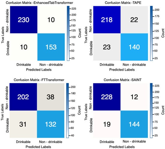
Figure 1. Confusion matrices depicting drinkable vs. non-drinkable water classification results using four transformer-based deep learning models: EnhancedTabTransformer, TAPE, FTTransformer, and SAINT.

As detailed in Table 3, the EnhancedTabTransformer demonstrated superior performance with an accuracy of 95.04% and an F1 score of 93.87%, establishing it as the most effective architecture for water potability classification among the evaluated models. ETT’s exceptional performance can be attributed to its sophisticated architecture, which leverages multi-head self-attention and hierarchical encoder layers to model complex, high-order interactions among physicochemical parameters. This aligns with the theoretical underpinnings of transformer models, which excel at capturing contextual dependencies through attention mechanisms [28].

Table 3. Performance metrics for the drinkable class—a comparative analysis of classification accuracies, F1 scores, and training times among state-of-the-art transformer-based models.

Model	Accuracy	F1 Score	Training Time (s)
EnhancedTabTransformer	0.9504	0.9387	540.45
TAPE	0.8883	0.8615	202.90
SAINT	0.9231	0.9028	789.18
FTTransformer	0.8289	0.7928	740.24

The SAINT architecture followed closely, with an accuracy of 92.31% and an F1 score of 90.28%, demonstrating its effectiveness in capturing both intra-feature and inter-sample relationships through its dual-attention mechanism. Its slightly lower accuracy compared to ETT may be due to its inter-sample attention, which increases training time (789.18 s vs. ETT’s 540.45 s, Table 3). This complexity, while enhancing the model’s ability to capture population-level patterns, may introduce sensitivity to batch composition, as inter-sample attention relies on contextual information from other samples in the batch [7].

TAPE exhibited moderate performance (88.83% accuracy, 86.15% F1 score), but demonstrated remarkable computational efficiency with the shortest training time (202.90 s), making it an attractive option for resource-constrained environments. However, its lower F1 score suggests that the pretraining phase, while effective at learning generalized representations, may not fully capture the detailed feature interactions that are critical for precise potability classification. The FTTransformer, despite its innovative feature tokenization approach, exhibited the lowest performance metrics (82.89% accuracy, 79.28% F1 score) while requiring considerable computational resources (740.24 s training time).

The detailed classification report for the EnhancedTabTransformer (Table 4) indicates highly balanced performance across both classes. The model achieved 96% precision, recall, and F1-score for the non-drinkable class and 94% for all metrics in the drinkable class.

Table 4. Classification report of the EnhancedTabTransformer model across two distinct classes.

	Precision	Recall	f1-Score	Support
Non-drinkable	0.96	0.96	0.96	240
Drinkable	0.94	0.94	0.94	163
Accuracy			0.95	403
Macro avg	0.95	0.95	0.95	403
Weighted avg	0.95	0.95	0.95	403

This balanced performance across classes is particularly valuable in water quality assessment applications, where both false positives (classifying non-potable water as potable) and false negatives (classifying potable water as non-potable) carry significant consequences for public health and resource management.

4.2. Feature Importance Analysis

Feature importance analysis (Table 5) revealed distinct patterns in how each architecture weighted the contribution of water quality parameters to potability classification. The EnhancedTabTransformer identified chloramines (0.102632) as the most significant parameter, followed by conductivity (0.075384), and trihalomethanes (0.070908). This aligns with established water quality standards, as chloramines serve as disinfection agents with strict regulatory thresholds due to their potential health impacts at elevated concentrations.

Table 5. Feature importances derived from top transformer-based deep neural network models.

Feature Importances
Transformer-Based Deep Neural Network Models
Features	ETabTransformer	TAPE	SAINT	FTTransformer
Chloramines (ppm)	0.102632	Could not extract weights for TAPE—no suitable layer found	0.163053	0.476386
Conductivity (MikroS/cm)	0.075384		0.152160	0.462036
Trihalomethanes (mikrog/L)	0.070908		0.139151	0.517876
ph	0.067879		0.194173	0.519935
Hardness (mg/L)	0.056796		0.169163	0.502482
Sulfate (mg/L)	0.056418		0.188918	0.564652
Turbidity (NTU)	0.054839		0.140685	0.454429
TDS solids (ppm = mg/L)	0.046426		0.172967	0.465583
Organic_carbon (ppm)	0.045725		0.156996	0.507146

The SAINT architecture assigned the highest importance to pH (0.194173), followed by sulfate (0.188918) and TDS solids (0.172967), suggesting that this model places greater emphasis on the chemical balance aspects of water quality. The FTTransformer displayed a more uniform distribution of feature importance values (ranging from 0.454429 to 0.564652), with sulfate (0.564652) receiving marginally higher importance. This more balanced feature weighting may partially explain the FTTransformer’s lower overall performance, as it might not sufficiently prioritize the most discriminative parameters.

The lower importance of features such as turbidity, total dissolved solids (TDS), and organic carbon across models suggests that these parameters may have less discriminatory power in this dataset. This could be attributed to their relatively narrow range of variation (e.g., turbidity: 1.45–6.49 NTU, Table 5) or their indirect relationship to potability compared to chloramines and trihalomethanes, which are directly linked to health risks. These insights can guide sensor prioritization in water quality monitoring systems, focusing resources on measuring high-impact parameters to optimize cost and efficiency. Unfortunately, feature importance values could not be extracted for the TAPE architecture due to its complex autoencoder structure, which does not contain a suitable layer for direct weight interpretation. This highlights a limitation in model interpretability for certain deep learning architectures, particularly those employing unsupervised pretraining methodologies.

4.3. Performance with Feature Subsets

The comparative analysis using different feature subsets (Table 6) provides critical insights into model robustness and the predictive power of specific parameter combinations. All models performed best when utilizing the full set of nine features (configuration 1*), confirming that comprehensive water quality assessment benefits from considering the full spectrum of physicochemical parameters. However, the performance degradation observed across different subset configurations varied significantly between models, revealing interesting patterns in architectural robustness.

Table 6. Comparative classification performance of top transformer-based deep neural network models on different feature subsets of the Water_Potability dataset.

Model	Acc 1* (%)	Acc 2* (%)	Acc 3* (%)	Acc 4* (%)	Acc 5* (%)
EnhancedTabTransformer	95.04	62.53	68.73	59.55	72.95
TAPE	88.83	65.51	63.52	59.55	75.93
SAINT	92.31	43.18	59.31	41.44	45.91
FTTransformer	82.88	60.79	58.81	40.45	54.84

The water_potability dataset consists of nine features: ‘ph’, ‘Hardness (mg/L)’, ‘TDS Solids (ppm = mg/L)’, ‘Chloramines (ppm)’, ‘Sulfate (mg/L)’, ‘Conductivity (µS/cm)’, ‘Organic_carbon (ppm)’, ‘Trihalomethanes (µg/L)’, and ‘Turbidity (NTU)’. In this study, transformer-based deep neural network models were evaluated using different combinations of these features to assess their classification performance. In the first configuration (1*), all nine features were used. The second configuration (2*) utilized a subset of four features: ‘ph’, ‘Chloramines (ppm)’, ‘Trihalomethanes (µg/L)’, and ‘Turbidity (NTU)’. The third configuration (3*) included ‘Chloramines (ppm)’, ‘Organic_carbon (ppm)’, ‘Trihalomethanes (µg/L)’, and ‘Sulfate (mg/L)’. The fourth configuration (4*) focused on three features: ‘ph’, ‘Trihalomethanes (µg/L)’, and ‘Turbidity (NTU)’. Lastly, the fifth configuration (5*) comprised ‘ph’, ‘Hardness (mg/L)’, ‘Chloramines (ppm)’, and ‘Sulfate (mg/L)’. These configurations were designed to investigate the impact of different feature subsets on model performance and to identify the most informative combinations for classifying drinkable and non-drinkable water samples.

The EnhancedTabTransformer maintained the highest accuracy across most subset configurations, with its performance dropping from 95.04% with all features to 72.95% in configuration 5* (pH, hardness, chloramines, and sulfate). This relatively smaller performance decline compared to other models suggests superior feature extraction capabilities that can maintain discriminative power even with reduced input dimensionality.

The TAPE architecture demonstrated remarkable resilience in configuration 5*, achieving the highest accuracy (75.93%) among all models for this specific feature subset. This indicates TAPE’s effective representation learning capabilities for these particular parameters, possibly attributable to its autoencoder-based pretraining that captures intrinsic structural relationships between these specific water quality indicators.

Reducing the feature set to subsets such as configuration 2* or configuration 5* led to significant performance degradation, particularly for the SAINT and FTTransformer models. This highlights the importance of diverse feature representation in capturing complex relationships within water quality data. The SAINT exhibited dramatic performance deterioration across all subset configurations, with accuracy dropping from 92.31% with all features to as low as 41.44% in configuration 4* (pH, trihalomethanes, and turbidity). This suggests that SAINT’s dual-attention mechanism might be optimized for higher-dimensional input spaces where complex feature interactions can be leveraged more effectively. The FTTransformer displayed moderate performance degradation across subset configurations, maintaining relatively consistent behavior but at lower overall accuracy levels. This indicates that while its feature tokenization approach provides stable performance characteristics, it may not extract sufficiently discriminative representations from the available water quality parameters compared to other architectures.

4.4. Statistical Analysis of Dataset Characteristics

The detailed statistical analysis of the water potability dataset (Table 7) reveals considerable variability across all measured parameters. pH values range from highly acidic (0.23) to strongly alkaline (14.00), with a mean of 7.09 approximating neutral conditions. This variability reflects the diverse sources and conditions under which water samples were collected.

Table 7. Data statistics of the water_potability dataset.

	ph	Hardness (mg/L)	TDS Solids (ppm = mg/L)	Chloramines (ppm)	Sulfate (mg/L)	Conductivity (MikroS/cm)	Organic_Carbon (ppm)	Trihalomethanes (mikrog/L)	Turbidity (NTU)
count	2011.0	2011.0	2011.0	2011.0	2011.0	2011.0	2011.0	2011.0	2011.0
mean	7.09	95.97	21,917.44	7.13	333.22	426.53	14.36	66.40	3.97
std	1.57	32.64	8642.24	1.58	41.26	80.71	3.32	16.08	0.78
min	0.23	73.49	320.94	1.39	129.00	201.62	2.20	8.58	1.45
25%	6.09	176.75	15,615.67	6.14	307.63	366.68	12.12	55.95	3.44
50%	7.03	197.19	20,933.51	7.14	332.23	423.46	14.32	66.54	3.97
75%	8.05	216.44	27,182.59	8.11	359.33	482.37	16.68	77.29	4.51
max	14.00	317.34	56,488.67	13.13	481.03	753.34	27.01	124.00	6.49

Total dissolved solids (TDS) demonstrate particularly high variability (standard deviation of 8642.24 ppm), ranging from 320.94 ppm to 56,488.67 ppm, indicating that the dataset encompasses water samples from diverse sources with varying mineral content. Chloramines, identified as the most important feature by the EnhancedTabTransformer, show concentrations ranging from 1.39 ppm to 13.13 ppm (mean: 7.13 ppm), with several samples exceeding regulatory limits for drinking water in many jurisdictions. Similarly, trihalomethanes, byproducts of water chlorination associated with potential health risks, range from 8.58 µg/L to 124.00 µg/L, with approximately 25% of samples exceeding the 80 µg/L threshold established by some regulatory agencies.

The substantial variability in water quality parameters underscores the complexity of the classification task and highlights the value of advanced machine learning approaches in capturing non-linear relationships between multiple physicochemical parameters and water potability.

4.5. Implications and Applications

The superior performance of transformer-based architectures, particularly the ETT and SAINT, demonstrates the efficacy of attention mechanisms in capturing complex relationships between water quality parameters. ETT, in particular, offers to achieve 95.04% of predictive accuracy, computational efficiency, and interpretability, making it suitable for deployment in diverse settings where comprehensive laboratory testing is challenging. Its ability to highlight key physicochemical parameters such as chloramines and conductivity can inform the design of targeted sensor arrays, reducing the complexity and cost of monitoring infrastructure. SAINT’s dual-attention mechanism, while computationally intensive, provides a unique advantage in capturing population-level patterns, which could be leveraged in large-scale environmental studies involving multiple water sources.

TAPE’s efficiency and competitive accuracy make it an appealing choice for scenarios with limited computational resources or unlabeled data, such as preliminary water quality assessments in developing regions. However, its lower F1 score suggests that further optimization, potentially through hybrid pretraining strategies, is needed to match ETT’s precision. Although FTTransformer is theoretically promising, its relatively poor performance in this study highlights the difficulty of applying transformer models to tabular data without careful hyperparameter tuning. This finding aligns with prior research indicating that transformer models can be sensitive to dataset characteristics and tuning [4].

The feature importance analysis provides valuable insights for practical applications in water quality monitoring. The identification of chloramines, pH, and sulfate as highly influential parameters across multiple models suggests these could serve as priority indicators in rapid screening protocols. This could inform the development of more targeted and cost-effective monitoring approaches, particularly in regions where comprehensive water quality assessment resources are limited.

Comparative analysis using feature subsets further supports this application potential, demonstrating that even with reduced parameter sets, transformer-based models can maintain reasonable classification accuracy. Configuration 5* (pH, hardness, chloramines, and sulfate) yielded the highest accuracy among all subset configurations across models, suggesting this combination of parameters might offer an optimal balance between measurement simplicity and predictive power for field deployment scenarios.

4.6. Limitations and Future Research Directions

Despite the promising results, several limitations and challenges deserve careful consideration. For example, groundwater in dry regions may exhibit different physicochemical characteristics than surface water in temperate zones. Future studies should validate these architectures across diverse water quality datasets representing multi-regional and contamination scenarios.

The interpretability challenges encountered with the TAPE architecture highlight ongoing limitations in translating complex deep learning models into actionable water quality management insights. Developing more transparent autoencoder-based approaches could enhance the utility of these models in regulatory and public health contexts where decision justifications are critical.

Additionally, while the current study focused on binary potability classification, future work could explore multi-class approaches that differentiate between various treatment requirements (e.g., no treatment, conventional treatment, and advanced treatment) or specific contamination types, providing more nuanced guidance for water resource management. The study did not account for temporal dynamics in water quality, which are critical for detecting seasonal variations or event-driven contamination (e.g., heavy rainfall or industrial spills).

5. Conclusions

This comparative study focused on four advanced transformer-based deep learning models aimed at classifying water potability from physicochemical features. The experimental results indicate clear performance differences between the architectures, with enhanced tabular transformers (ETT) showing the best performance. The ETT achieved a test accuracy of nearly 95%, significantly outperforming the other models (SAINT: ~92%, TAPE: ~89%, and FTTransformer: ~83%). The F1-score of ETT (≈0.94) was likewise the highest among these, which points to its excellent precision–recall balance for drinkable and non-drinkable inferences.

Specifically, multi-head self-attention and efficient feature embeddings combined within the enhanced tabular transformer proved very beneficial for the binary classification task. The strong performance of the SAINT continues to resonate with previous reports touting its strengths, emphasizing the importance of its dual-attention mechanism, although it ranked just short of ETT in our evaluations. The TAPE model achieved competitive results aided by an unsupervised autoencoder pre-training phase, suggesting this pre-training helped, although it certainly could not rival ETT’s fully supervised approach.

Meanwhile, the FTTransformer—albeit easy and theoretically powerful on some benchmarks, was the underperformer in this study, perhaps owing to extensive hyperparameter tuning or difficulties associated with the water potability data that are very highly imbalanced. All in all, the study establishes that transformer-based deep learning frameworks are not only feasible but are among the most effective for water quality classification. The enhanced tabular transformer could be a strong basis for the development of intelligent water monitoring systems due to the state-of-the-art results it achieved on the dataset tested. Such findings serve to motivate the further embrace of advanced deep learning in environmental informatics, especially in high-risk applications such as the drinking water safety assessment. Concurrently, the study indicated that one model cannot be simply the best across the board; architecture selection must be relevant to the characteristics of the dataset and constraints in computational resources (for example, SAINT took longer to train due to its elaborate attention, whereas TAPE trained relatively fast but was a bit less accurate).

Future Directions

Multimodal data integration with temporal modeling: Future research may focus on the integration of temporal sensor data (e.g., hourly turbidity, and hourly temperature trends) through sequence-aware architecture designs, such as hybrid models wherein LSTM and transformers are mixed or through temporal fusion transformers (TFT). These models, being capable of addressing time-dependent procedural changes in water quality, will also become useful for appraising very dynamic environmental prediction scenarios. Real-life effectiveness can be checked through benchmarking on time-stamped datasets.

Recent computer vision research indicates that transformer variants may boast the ability to generalize across domains. Hwang et al. (2025) [25] implemented transformer-compatible data augmentation and instance-based segmentation methods in estimating the dimensions of buildings in urban scenes; Park et al. (2025) [27] incorporated advanced image enhancement techniques into transformer models of YOLOv8 to detect PPEs at construction sites. Though stemming from visual realms, the transformer-based approaches have much to offer in cross-domain adaptability and robustness, thereby implying that analog methods may also come in handy for environmental forecast studies such as water quality modeling.

Cross-domain generalization with meta-learning: To tackle the regional variability for the water sources, meta-learning algorithms (for example, MAML or Reptile) can be exercised to enhance cross-site adaptability. Fine-tuning transformer models from a few-shot samples from new locations may enforce robust generalization. The performance should be tested on a dataset from geologically different regions, for example, urban vs. rural vs. coastal settings.

Feature attribution via SHAP and integrated gradients: Whereas the interpretation of attention weights shed some light on the issue, the next steps should apply other model-agnostic interpretation methods, such as SHAP and integrated gradients to ETT and SAINT. These methods should then be able to uncover both global and local feature influences in artifacts as they would help clarify end-users the way parameters, such as pH, turbidity, or TDS, come into play in potable decisions. A comparison of interpretability methods could yield valuable insights as well.

Model compression and edge deployment: Since monitoring water might eventually occur in remote or resource-starved locales, research would also develop model-compression techniques, including pruning, quantization, and knowledge distillation, for deploying these models onto edge devices with low power. Experiments may focus on the trade-offs between inference speed and model size, and predictive accuracy.

Resistance to sensor interference and data loss: Deep models should also be examined in terms of the presence of noise, drops, and time delays in adding sensor data. Dropout methods, robust objectives, or possible Bayesian transformers (e.g., BERT with uncertainty estimation) could be applied to such conditions. Testing such under-constrained noise conditions will highlight the boundaries in operation.

Open-source benchmark and standardized evaluation: Prior work also recommended that future research focus on the creation of open-source benchmarks for the classification of water quality. The opening up of the datasets, model implementations, and evaluation pipelines will go a long way toward enhancing experiment reproducibility and more consistent comparisons across studies.

References

- World Health Organization. Drinking-Water. 2023. Available online: https://www.who.int/news-room/fact-sheets/detail/drinking-water (accessed on 12 April 2025).
- Patel, S.; Shah, K.; Vaghela, S.; Aglodiya, M.; Bhattad, R. Water Potability Prediction Using Machine Learning. Preprints 2023, 2023052965. [Google Scholar] [CrossRef]
- Bellur, A.P.; VL, V.K.; Choudary, S.K.; Kodipalli, A.; Rao, T.; Pushpalatha, V. Water Quality Assessment Using Machine Learning: A Comparative Analysis. In Proceedings of the 2023 International Conference on Computational Intelligence for Information, Security and Communication Applications (CIISCA), Bengaluru, India, 10–11 March 2023; pp. 320–325. [Google Scholar] [CrossRef]
- Gorishniy, Y.; Rubachev, I.; Khrulkov, V.; Babenko, A. Revisiting Deep Learning Models for Tabular Data. arXiv 2021, arXiv:2106.11959. Available online: https://arxiv.org/abs/2106.11959 (accessed on 12 April 2025).
- Arik, S.Ö.; Pfister, T. TabNet: Attentive Interpretable Tabular Learning. Proc. AAAI Conf. Artif. Intell. 2021, 35, 6679–6687. [Google Scholar] [CrossRef]
- Huang, X.; Khetan, A.; Cvitkovic, M.; Karnin, Z. TabTransformer: Tabular Data Modeling Using Contextual Embeddings. arXiv 2020, arXiv:2012.06678. [Google Scholar] [CrossRef]
- Somepalli, G.; Goldblum, M.; Schwarzschild, A.; Bruss, C.B.; Goldstein, T. SAINT: Improved Neural Networks for Tabular Data via Row Attention and Contrastive Pre-Training. arXiv 2021, arXiv:2106.01342. [Google Scholar] [CrossRef]
- Amarbayasgalan, T.; Pham, V.H.; Theera-Umpon, N.; Ryu, K.H. Unsupervised Anomaly Detection Approach for Time-Series in Multi-Domains Using Deep Reconstruction Error. Symmetry 2020, 12, 1251. [Google Scholar] [CrossRef]
- Jijo, B.T.; Abdulazeez, A.M. Classification Based on Decision Tree Algorithm for Machine Learning. J. Appl. Sci. Technol. Trends 2021, 2, 20–28. [Google Scholar] [CrossRef]
- Uddin, M.G.; Nash, S.; Rahman, A.; Olbert, A.I. Performance Analysis of the Water Quality Index Model for Predicting Water State Using Machine Learning Techniques. Process Saf. Environ. Prot. 2023, 169, 808–828. [Google Scholar] [CrossRef]
- Sun, Z.; Wang, G.; Li, P.; Wang, H.; Zhang, M.; Liang, X. An Improved Random Forest Based on the Classification Accuracy and Correlation Measurement of Decision Trees. Expert Syst. Appl. 2024, 237, 121549. [Google Scholar] [CrossRef]
- Chen, T.; Guestrin, C. XGBoost: A Scalable Tree Boosting System. In Proceedings of the 22nd ACM SIGKDD International Conference on Knowledge Discovery and Data Mining, San Francisco, CA, USA, 13–17 August 2016; pp. 785–794. [Google Scholar] [CrossRef]
- Kuthe, A.; Bhake, C.; Bhoyar, V.; Yenurkar, A.; Khandekar, V.; Gawale, K. Water Quality Prediction Using Machine Learning. Int. J. Comput. Sci. Mob. Comput. 2023, 12, 52–59. [Google Scholar] [CrossRef]
- Dong, J.; Chen, Y.; Yao, B.; Zhang, X.; Zeng, N. A Neural Network Boosting Regression Model Based on XGBoost. Appl. Soft Comput. 2022, 125, 109067. [Google Scholar] [CrossRef]
- Chen, W.; Xu, D.; Pan, B.; Zhao, Y.; Song, Y. Machine Learning-Based Water Quality Classification Assessment. Water 2024, 16, 2951. [Google Scholar] [CrossRef]
- Grinsztajn, L.; Oyallon, E.; Varoquaux, G. Why Do Tree-Based Models Still Outperform Deep Learning on Tabular Data? arXiv 2022, arXiv:2207.08815. Available online: https://arxiv.org/abs/2207.08815 (accessed on 14 April 2025).
- Bengio, Y.; Courville, A.; Vincent, P. Representation Learning: A Review and New Perspectives. IEEE Trans. Pattern Anal. Mach. Intell. 2013, 35, 1798–1828. [Google Scholar] [CrossRef] [PubMed]
- Erhan, D.; Courville, A.; Bengio, Y.; Vincent, P. Why Does Unsupervised Pre-Training Help Deep Learning? In Proceedings of the Thirteenth International Conference on Artificial Intelligence and Statistics (AISTATS), Chia Laguna Resort, Sardinia, Italy, 13–15 May 2010; pp. 201–208. [Google Scholar]
- Akhlaq, M.; Ellahi, A.; Niaz, R.; Khan, M.; Sammen, S.S.; Scholz, M. Comparative Analysis of Machine Learning Algorithms for Water Quality Prediction. Tellus A Dyn. Meteorol. Oceanogr. 2024, 76, 177–192. [Google Scholar] [CrossRef]
- Wang, K.; Liu, L.; Ben, X.; Jin, D.; Zhu, Y.; Wang, F. Hybrid Deep Learning Based Prediction for Water Quality of Plain Watershed. Environ. Res. 2024, 262 Pt 2, 119911. [Google Scholar] [CrossRef]
- Sekarlangit, S.; Widodo, C.E.; Tarno, T. A Comparison of Artificial Neural Network (ANN) and Long Short-Term Memory (LSTM) in River Water Quality Prediction. Int. J. Curr. Sci. Res. Rev. 2024, 7, 11–18. [Google Scholar] [CrossRef]
- Gan, M.; Pan, S.; Chen, Y.; Cheng, C.; Pan, H.; Zhu, X. Application of the Machine Learning LightGBM Model to the Prediction of the Water Levels of the Lower Columbia River. J. Mar. Sci. Eng. 2021, 9, 496. [Google Scholar] [CrossRef]
- Li, L.; Gu, Z. Research on Surface Water Quality Prediction Based on a CNN-BiLSTM-Attention Combined Deep Learning Approach. E3S Web Conf. 2023, 393, 01007. [Google Scholar] [CrossRef]
- Gymprathap, K.; Water Quality Dataset. Data.World. 2023. Available online: https://data.world/gymprathap/water-quality-dataset (accessed on 12 April 2025).
- Little, R.J.A.; Donald, B.R. Statistical Analysis with Missing Data; John Wiley & Sons: Hoboken, NJ, USA, 2019. [Google Scholar]
- Hastie, T.; Tibshirani, R.; Friedman, J. The Elements of Statistical Learning; Springer: New York, NY, USA, 2009. [Google Scholar]
- Norris, J.R. Markov Chains; No. 2; Cambridge University Press: Cambridge, UK, 1998. [Google Scholar]
- Vaswani, A.; Shazeer, N.; Parmar, N.; Uszkoreit, J.; Jones, L.; Gomez, A.N.; Kaiser, Ł.; Polosukhin, I. Attention Is All You Need. Adv. Neural Inf. Process. Syst. 2017, 30, 5998–6008. [Google Scholar]
- Hendrycks, D.; Gimpel, K. Gaussian Error Linear Units (GELUs). arXiv 2016, arXiv:1606.08415. Available online: https://arxiv.org/abs/1606.08415 (accessed on 12 April 2025).
- Samek, W.; Montavon, G.; Vedaldi, A.; Hansen, L.K.; Müller, K.-R. (Eds.) Explainable AI: Interpreting, Explaining and Visualizing Deep Learning; Springer Nature: Cham, Switzerland, 2019; Volume 11700. [Google Scholar]
Disclaimer/Publisher’s Note: The statements, opinions and data contained in all publications are solely those of the individual author(s) and contributor(s) and not of MDPI and/or the editor(s). MDPI and/or the editor(s) disclaim responsibility for any injury to people or property resulting from any ideas, methods, instructions or products referred to in the content. |
© 2025 by the authors. Licensee MDPI, Basel, Switzerland. This article is an open access article distributed under the terms and conditions of the Creative Commons Attribution (CC BY) license (https://creativecommons.org/licenses/by/4.0/).